A multivariate Bayesian learning approach for improved detection of doping in athletes using urinary steroid profiles

Abstract

Biomarker analysis of athletes’ urinary steroid profiles is crucial for the success of anti-doping efforts. Current statistical analysis methods generate personalised limits for each athlete based on univariate modelling of longitudinal biomarker values from the urinary steroid profile. However, simultaneous modelling of multiple biomarkers has the potential to further enhance abnormality detection. In this study, we propose a multivariate Bayesian adaptive model for longitudinal data analysis, which extends the established single-biomarker model in forensic toxicology. The proposed approach employs Markov chain Monte Carlo sampling methods and addresses the scarcity of confirmed abnormal values through a one-class classification algorithm. By adapting decision boundaries as new measurements are obtained, the model provides robust and personalised detection thresholds for each athlete. We tested the proposed approach on a database of 229 athletes which includes longitudinal steroid profiles classified as normal, atypical, or confirmed abnormal. Our results demonstrate improved detection performance, highlighting the potential value of a multivariate approach in doping detection.

Keywords: Anti-doping, Bayesian adaptive model, biomarkers, decision boundaries, longitudinal data, Markov chain Monte Carlo, multivariate analysis, one-class classification, urinary steroid profile.

1 Introduction

Doping has been widely discussed in recent years and remains a challenging topic in the athletic world. In competitive sports, prohibited substances such as anabolic androgenic steroids (AAS), refer to the drugs that are closely associated with the notion of doping [1]. AAS are the most frequent detected class of substances in doping controls [2]. In order to detect the administration of endogenous steroids, i.e. steroids that are produced inside the body such as testosterone, the steroidal module of the Athlete Biological Passport (ABP) was developed [3]. The steroidal module is used to denote a follow-up which is the recording of the concentration of endogenous steroids and their ratios in urine over time. In order to establish the ABP, the World Anti-Doping Agency (WADA) provided harmonised and robust analytical methods for the “steroid profile” which according to their technical document (TD) [4] is composed of the following endogenous anabolic androgenic steroids (EAAS): testosterone (T), epitestosterone (E), androsterone (A), etiocholanolone (Etio), 5-androstane-3, 17-diol (A5), 5-androstane-3, 17-diol (B5), as well as the concentration ratios T/E, A/T, A/Etio, A5/B5 and A5/E. As the intra-individual variation of all these markers is much lower than the inter-individual variation in the population of athletes, individual longitudinal monitoring as applied by the ABP increases the sensitivity for the detection of illicit AAS administration. For each athlete an individual reference range is specified for each biomarker as samples are added to the ABP over time. If a new steroid profile enters into the individual ABP and values fall beyond established thresholds, the ABP alerts athlete passport management units (APMUs) that anomalies have been detected that require closer examination [3, 5, 6, 7]. Employing this approach, the ABP mostly aids in revealing the direct and indirect effects of doping with anabolic agents on the individual steroid profile rather than detecting the prohibited substance itself [8, 9]. Therefore, further steps during the closer examination encompass steroid profile confirmation, detection of confounding factors and isotope ratio mass spectrometry (IRMS) based investigations. By far the most commonly used screening tool in sports drug testing over the last years uses the T/E ratio, as it is considered a stable marker ratio within an athlete’s steroid profile, sensitive to the administration of T itself and T-prohormones [10]. Measuring only the urinary T concentrations has proved inadequate due to the small ratio of intra- to inter-individual variability in the urinary steroid concentrations caused by various factors [11, 12, 13, 14, 10]. Therefore, monitoring the steroid profile at individual level is very important, mostly because the reference values based on the population do not always have the sensitivity to track whether anabolic drugs have been administered [15, 16]. Current approaches receive new measurements of a single biomarker or ratio and, under a Bayesian framework, progressively adapt population-derived limits, when there are no recorded measurements, to individual normal ranges as the number of measurements increases [17]. Multivariate statistical approaches have also been proposed for this purpose, which are able to combine population information with individual longitudinal monitoring of multiple biomarkers [18, 19, 20]. However, multivariate statistical methods in a Bayesian adaptive framework have not yet been attempted. This research focuses on the development of an improved statistical model for classifying athletes’ urine samples into suspicious and non-suspicious classes. The classification technique is based on comparisons of sequential measurements of a set of biological variables against previous recordings. For this purpose, we gradually move from the univariate to a multivariate statistical model which considers prior information on inter- and intra-individual variations, and on potential correlation between the EAAS markers. A fully validated method using GC-MS analysis and fulfilling all requirements as per TD EAAS [10, 4] determined the six markers and the five ratios which compose the urinary steroid profile of the ABP of 229 athletes. Out of them, 100 were athletes whose samples are considered to be normal (i.e. none of their samples was found beyond the individual limits), 100 were athletes with one or more extreme samples classified as atypical (i.e. samples beyond the individual limits but in none of these a doping offence was detectable), and 29 confirmed dopers, each marked with at least one atypical sample in their longitudinal steroid profile and confirmed to be a real doping offence employing IRMS according to WADA regulation [21]. The latter samples are classified as abnormal. These EAAS concentrations were longitudinally sampled from professional athletes, whereas cross-sectional measurements of the same markers and ratios from a baseline population of 164 healthy and non-doped volunteers were used to extract prior information for the normal range of steroid concentrations. It is worth noting that recordings from athletes with normal concentration values are more readily available than from doped athletes. Since the imbalance in size between the two classes is unavoidable, traditional classification methods may not work effectively as they are biased towards the predominant class. Hence, we classify athletes’ samples based on a one-class classification algorithm. The AAS concentrations from non-doped athletes define the “target” class for which adaptive decision boundaries are constructed to separate them from abnormal data (also known as outliers or anomalies). The remaining sections are structured as follows. In Section 2 we introduce two models; a univariate and a multivariate Bayesian adaptive model. The former can be applied to individual biomarkers or ratios within the steroid profile, while the latter is designed to analyse multiple biomarkers and/or ratios simultaneously. Section 3 describes the one-class classification method using the highest posterior predictive density (HPD). In Section 4 we present summaries of real athletes’ data and the HPD estimation on both models. The inference and computations in the analysis relied on either sampling from a known joint posterior distribution or sampling from a non-closed form distribution employing Markov chain Monte Carlo (MCMC) methods, depending on the model being used. The computer code for the developed models is written in the statistical language R 4.2.2 [22]. We compare the two models with each other but also assess them against a simpler generalised linear mixed effects model (GLMM) and the univariate Bayesian approach introduced by Sottas et al. [17], exclusively designed for the analysis of the T/E ratio. Furthermore, we conduct a comparison with the univariate Bayesian model applied to the Euclidean distance score as outlined in the work of de Figueiredo et al. [23]. Section 5 discusses the main findings and directions for further research.

2 Models

2.1 The univariate Bayesian model

In this section we introduce an expanded version of the univariate Bayesian model for the T/E ratio proposed by Sottas et al. [17] to a univariate Bayesian hierarchical model for any steroidal component or ratio of the ABP [24]. Under a Bayesian framework, the model receives new measurements and progressively adapts population-derived limits, when the number of measurements $n$ is zero, to individual normal ranges, when $n$ is large. Let $\boldsymbol{y}$ $=(y_{1},...,y_{n})$ represent the vector with the $n$ log-transformed recorded values of the biomarker $Y$ collected from the same athlete. It is important to mention that the period among two sequential samples of an athlete is long enough for them to be considered independent. Hence, we assume the logarithm of EAAS values to be a vector of $n$ independent and identically distributed draws from a Gaussian distribution with mean $\mu$ and variance $\sigma^{2}$, that is

$$Y|\mu,\sigma^{2}{\sim}\mathcal{N}(\mu,\sigma^{2}).$$ (1)

We focus on modelling the logarithm of these EAAS concentrations due to the fact that there are physical constraints on the measurement values (i.e. all markers are positive) and taking the logarithm allows us to use the Gaussian distribution in our models. To describe prior knowledge about the unknown parameters, i.e. the mean $\mu$ and the precision $\tau=1/\sigma^{2}$, we specify the joint prior distribution as the product of a conditional and a marginal distribution expressed as $p(\mu,\tau)=p(\mu|\tau)p(\tau)$. Given our limited prior information on the parameters of the model regarding the six available biomarkers and their five ratios with the exception of the T/E ratio, we propose specifying weakly informative conditionally conjugate priors on these model parameters. Therefore, a Gaussian distribution is assigned to the mean conditional on the precision as

$$\mu|\tau\sim\mathcal{N}(\mu_{0},1/(\kappa_{0}\tau)),$$ (2)

with hyper-parameters $\mu_{0}$ (prior mean) and $\kappa_{0}$ (prior sample size, which determines the tightness of the prior). The inverse of the variance is assumed to follow a conjugate Gamma prior distribution expressed as

$$\tau\sim\mathcal{G}a(\alpha_{0},\beta_{0}),$$ (3)

where $\alpha_{0}$ and $\beta_{0}$ determine the shape and rate hyper-parameters, respectively. The T/E ratio is excluded from the semi-informative prior setting because there is adequate population information regarding its characteristics given by Sottas et al. [17]. However, we present the analysis results of T/E using both informative and weakly informative priors for comparison purposes. As a conjugate family, the joint posterior distribution for the pair of parameters $(\mu,\tau)$ is also a Gaussian-Gamma distribution

$$\mu,\tau|\boldsymbol{y}\sim\mathcal{NG}a(\mu_{n},\kappa_{n},\alpha_{n},\beta_{n}),$$ (4)

where the index $n$ on the hyper-parameters indicates the updated values after seeing the $n$ observations from the sample data, that is

$$\begin{split}\kappa_{n}&=\kappa_{0}+n,\hskip 14.22636pt\mu_{n}=\frac{\kappa_{0}\mu_{0}+n\bar{y}}{\kappa_{n}},\\ \alpha_{n}&=\alpha_{0}+n/2,\hskip 14.22636pt\beta_{n}=\beta_{0}+\frac{1}{2}\sum_{i=1}^{n}(y_{i}-\bar{y})^{2}+\frac{\kappa_{0}n}{2\kappa_{n}}(\bar{y}-\mu_{0})^{2}.\end{split}$$

2.2 Proposed multivariate Bayesian adaptive model

In Sottas et al. [17], the T/E marker is modelled by a univariate Gaussian distribution in a Bayesian context. In this section, we present a multivariate Bayesian adaptive model (MBA), which can deal with a wide variety of markers in their logarithmic scale as a generalisation of the univariate model of [17]. The MBA is expressed as

$$y_{ijk}=\mu_{k}+b_{jk}+e_{ijk},\,\,\,\,\boldsymbol{b_{j}}\overset{\text{iid}}{\sim}\mathcal{N}_{K}(\boldsymbol{0},\Omega_{b}^{-1}),\,\,\,\,\boldsymbol{e}_{ij}\overset{\text{iid}}{\sim}\mathcal{N}_{K}(\boldsymbol{0},\Omega_{e}^{-1}),$$ (5)

where $y_{ijk}$ denotes the logarithm of the $i$th observation of the $k$th marker for the $j$th athlete, $\mu_{k}$ is the fixed effect for the overall mean of all observations of $k$th response marker, $b_{jk}$ is the random effect of athlete $j$ for the $k$th marker, and $e_{ijk}$ is the random term for other variation in its $i$th measurement, while $i=1,...,n_{j}$, $j=1,...,J$ and $k=1,...,K$. The assumptions here are that for a certain marker $k$, the random effects $b_{jk}$ are independent, identically and normally distributed between subjects and the error terms $e_{ijk}$ are also independent, identically and normally distributed between and within subjects. Shorthand notation for the overall mean is $\boldsymbol{\mu}=\{\mu_{k}\}_{k=1}^{K}$ and for the random effects is $\boldsymbol{b}=\{\boldsymbol{b_{j}}\}_{j=1}^{J}=\{b_{jk}\}_{j=1\,\,k=1}^{J\,\,\,\,K}$. The precision matrices are denoted by $\Omega_{\mu}$ and $\Omega_{e}$ for the overall mean $\boldsymbol{\mu}$ and for the error term $\boldsymbol{e}_{ij}$, respectively. $\Omega_{b}$ is the precision matrix of $\boldsymbol{b_{j}}$, which captures the correlation between the $K$ markers. Suppose we have the following Bayesian hierarchical multiple response model

$$\begin{split}\boldsymbol{y}_{ij}|\boldsymbol{\mu_{j}}&\overset{\text{iid}}{\sim}\mathcal{N}_{K}(\boldsymbol{\mu_{j}}=\boldsymbol{\mu}+\boldsymbol{b_{j}},\,\Omega_{e}^{-1})\\ \boldsymbol{\mu}\,|\boldsymbol{\mu_{0}}&\overset{\text{iid}}{\sim}\mathcal{N}_{K}(\boldsymbol{\mu_{0}},\,\Omega_{\mu}^{-1})\\ \boldsymbol{b_{j}}&\overset{\text{iid}}{\sim}\mathcal{N}_{K}(\boldsymbol{0},\,\Omega_{b}^{-1})\\ \Omega_{e}&\overset{\text{iid}}{\sim}\mathcal{W}i(d_{e},S_{e})\\ \Omega_{\mu}&\overset{\text{iid}}{\sim}\mathcal{W}i(d_{\mu},S_{\mu})\\ \Omega_{b}&\overset{\text{iid}}{\sim}\mathcal{W}i(d_{b},S_{b}),\end{split}$$ (6)

where the overall mean $\boldsymbol{\mu}$ and the random effects $\boldsymbol{\mu_{j}}$ have conjugate multivariate Gaussian priors, while the precision matrices $\Omega_{e}$, $\Omega_{\mu}$ and $\Omega_{b}$ have conjugate Wishart priors. Historical prior information about all response variables is captured by the prior mean vector $\boldsymbol{\mu_{0}}$. Moreover, $d_{e}$, $d_{\mu}$ and $d_{b}$ denote the degrees of freedom, and $S_{e}$, $S_{\mu}$ and $S_{b}$ are the prior covariance matrices which are selected such that their corresponding prior distributions will be non-informative. The degrees of freedom of the Wishart distribution need to be greater than the data dimension minus one, i.e. $d_{e}>K-1$, so a non-informative value for this parameter is chosen to be equal to $K$ [25]. The prior covariance matrices $S_{e}$, $S_{\mu}$ and $S_{b}$ are all set equal to $(1/1000)\mathbb{I_{K}}$ so that posterior inferences would be largely driven by the data. A graphical representation of the MBA is shown in Figure 1.

Figure 1: A graphical representation of MBA with conjugate priors. The overall mean, $\boldsymbol{\mu}$, and the precision matrix, $\Omega_{e}$, are assumed to be independent.

We approximate the posterior parameters by using Gibbs sampling [26, 27]. To apply the Gibbs sampler (see Algorithm 1), the full conditional posterior distributions for each of the unknown parameters of $\boldsymbol{\theta}=(\boldsymbol{\mu},\{\boldsymbol{\mu_{j}}\}_{j=1}^{J},\Omega_{e},\Omega_{\mu},\Omega_{b})$ are calculated as follows:

$$\begin{split}\boldsymbol{\mu}|\{\boldsymbol{\mu_{j}}\}_{j=1}^{J},\Omega_{e},\Omega_{\mu},\Omega_{b},\boldsymbol{y}&\sim\mathcal{N}_{K}(A_{n}^{-1}b_{n},\,A_{n}^{-1})\\ \boldsymbol{\mu_{j}}|\boldsymbol{\mu},\boldsymbol{\mu_{-j}},\Omega_{e},\Omega_{\mu},\Omega_{b},\boldsymbol{y}&\sim\mathcal{N}_{K}(A_{n}^{{}^{\prime}-1}b_{n}^{\prime},\,A_{n}^{{}^{\prime}-1})\,\,\,\forall\,\,j=1,...,J\\ \Omega_{e}|\{\boldsymbol{\mu_{j}}\}_{j=1}^{J},\boldsymbol{\mu},\Omega_{\mu},\Omega_{b},\boldsymbol{y}&\sim\mathcal{W}i(d_{e}^{\prime},S_{e}^{\prime})\\ \Omega_{\mu}|\{\boldsymbol{\mu_{j}}\}_{j=1}^{J},\boldsymbol{\mu},\Omega_{e},\Omega_{b},\boldsymbol{y}&\sim\mathcal{W}i(d_{\mu}^{\prime},S_{\mu}^{\prime})\\ \Omega_{b}|\{\boldsymbol{\mu_{j}}\}_{j=1}^{J},\boldsymbol{\mu},\Omega_{e},\Omega_{\mu},\boldsymbol{y}&\sim\mathcal{W}i(d_{b}^{\prime},S_{b}^{\prime}),\end{split}$$ (7)

where in this section $\boldsymbol{y}$ is a $n_{j}\times J\times K$ data matrix and

$$A_{n}=J\Omega_{b}+\Omega_{\mu},\hskip 14.22636ptb_{n}=\Omega_{\mu}\boldsymbol{\mu_{0}}+J\Omega_{b}\boldsymbol{\bar{\mu}},\hskip 14.22636pt\boldsymbol{\bar{\mu}}=\frac{1}{J}\sum_{j=1}^{J}\boldsymbol{\mu_{j}},$$

$$A_{n}^{\prime}=\Omega_{b}+n_{j}\Omega_{e},\hskip 14.22636ptb_{n}^{\prime}=\Omega_{b}\boldsymbol{\mu}+\Omega_{e}\sum_{i=1}^{n_{j}}\boldsymbol{y_{ij}},$$

$$d_{e}^{\prime}=d_{e}+n,\hskip 14.22636ptn=\sum_{j=1}^{J}n_{j},\hskip 14.22636ptS_{e}^{\prime}=S_{e}^{-1}+\sum_{j=1}^{J}\sum_{i=1}^{n_{j}}(\boldsymbol{y_{ij}}-\boldsymbol{\mu_{j}})(\boldsymbol{y_{ij}}-\boldsymbol{\mu_{j}})^{T},$$

$$d_{\mu}^{\prime}=d_{\mu}+1,\hskip 14.22636ptS_{\mu}^{\prime}=S_{\mu}^{-1}+(\boldsymbol{\mu}-\boldsymbol{\mu_{0}})(\boldsymbol{\mu}-\boldsymbol{\mu_{0}})^{T},$$

$$d_{b}^{\prime}=d_{b}+J,\hskip 14.22636ptS_{b}^{\prime}=S_{b}^{-1}+\sum_{j=1}^{J}(\boldsymbol{\mu_{j}}-\boldsymbol{\mu})(\boldsymbol{\mu_{j}}-\boldsymbol{\mu})^{T}.$$

Algorithm 1 Gibbs algorithm

1: Generate an initial state $\boldsymbol{\theta}^{(0)}=(\boldsymbol{\mu}^{(0)},\{\boldsymbol{\mu_{j}}^{(0)}\}_{j=1}^{J},\Omega^{(0)}_{e},\Omega^{(0)}_{\mu},\Omega^{(0)}_{b})$

2:for $t\leftarrow 1\textrm{ to }T$ do

3:draw $\boldsymbol{\mu}^{(t)}\,\,\sim p(\boldsymbol{\mu}\,|\{\boldsymbol{\mu}^{(t-1)}_{j}\}_{j=1}^{J},\,\Omega_{e}^{(t-1)},\Omega_{\mu}^{(t-1)},\Omega_{b}^{(t-1)},\boldsymbol{y})$

4:    for $j\leftarrow 1\textrm{ to }J$ do

5:      draw $\boldsymbol{\mu_{j}}^{(t)}\,\,\sim p(\boldsymbol{\mu}_{j}\,|\boldsymbol{\mu}^{(t)},\boldsymbol{\mu}_{-j}^{(t-1)},\,\Omega_{e}^{(t-1)},\Omega_{\mu}^{(t-1)},\Omega_{b}^{(t-1)},\boldsymbol{y})$

6:    end for

7:draw $\Omega^{(t)}_{e}\sim p(\Omega_{e}\,|\,\boldsymbol{\mu}^{(t)},\{\boldsymbol{\mu_{j}}^{(t)}\}_{j=1}^{J},\Omega_{\mu}^{(t-1)},\Omega_{b}^{(t-1)},\boldsymbol{y})$

8:draw $\Omega^{(t)}_{\mu}\sim p(\Omega_{\mu}\,|\,\boldsymbol{\mu}^{(t)},\{\boldsymbol{\mu_{j}}^{(t)}\}_{j=1}^{J},\Omega_{e}^{(t)},\Omega_{b}^{(t-1)},\boldsymbol{y})$

9:draw $\Omega^{(t)}_{b}\sim p(\Omega_{b}\,|\,\boldsymbol{\mu}^{(t)},\{\boldsymbol{\mu_{j}}^{(t)}\}_{j=1}^{J},\Omega_{e}^{(t)},\Omega_{\mu}^{(t)},\boldsymbol{y})$

10:end for

3 Methodology

3.1 One-class classification

One-class classification (OCC) algorithms are used in classification when only one class (known as “target” class) is fully known and the others are either absent or poorly sampled [28, 29, 30]. Doping detection constitutes a challenging topic in forensic toxicology, and can be framed as a one-class classification problem since measurements from doped athletes can be difficult to obtain, either due to the elaborated techniques that athletes use to avoid testing, or due to the undetectable use of banned substances.

For doping analysis, full information is provided on non-doped athletes who have been voluntarily tested, but limited knowledge is available for athletes who have received doping regimens. Thus, the samples from athletes with normal concentration values are treated as the “target” class. The focus is on studying whether there is evidence that new samples from athletes, whose doping status is unknown, are compatible with the known normal class of samples, or whether they show an abnormal pattern and should be considered as outliers. A classifier, that is a function which assigns each input data point to a class, accounting for other confounding factors such as sex, cannot be constructed with known standard rules in the case of imbalanced classes. In a machine learning context, the main purpose is to infer a classifier from a limited set of training data noting that, in addition to the complexity of unbalanced data, the classifier should also have the capability to deal with longitudinal data, their updating nature as well as potential confounders. We approach the one-class classification problem using a density estimation method for OCC models in $K$-dimensional space as described in the following section.

3.2 Highest posterior predictive density

The Bayesian model specification contributes to hierarchically shift from the prior evidence about population parameters $\boldsymbol{\theta}$ to the revised knowledge, expressed in the posterior density $p(\boldsymbol{\theta}|\boldsymbol{y})$, as new data become available. Using MCMC sampling methods, we can estimate the posterior density function and then approximate the $K$-variate predictive density function of a $1\times K$ new observable vector $\boldsymbol{y_{n+1}}$ given the data $\boldsymbol{y}$ of dimensionality $n_{j^{\prime}}\times J^{\prime}\times K$, where $J^{\prime}=J+1$. Therefore, the predictive density function is calculated as

$$p(\boldsymbol{y_{n+1}}|\boldsymbol{y=\{Y_{0},Y\}})=\int_{\Theta}f(\boldsymbol{y_{n+1}}|\boldsymbol{\theta})p(\boldsymbol{\theta}|\boldsymbol{Y_{0},Y})d\boldsymbol{\theta},$$ (8)

which is formed by weighting the possible values of $\boldsymbol{\theta}$ in the future observation $f(\boldsymbol{y_{n+1}}|\boldsymbol{\theta})$ by how likely we believe they are to occur, $p(\boldsymbol{\theta}|\boldsymbol{y})$. Note that $\boldsymbol{y}$ consists of both data from the baseline normal population, $\boldsymbol{Y_{0}}^{n_{j}\times J\times K}$, and all previous $n$ normal recordings of the under study athlete $J^{\prime}$, $\boldsymbol{Y}^{n\times K}=(\boldsymbol{y_{1}},...,\boldsymbol{y_{n}})^{\top}$. We can use the predictive distribution to provide a useful range of plausible concentration values for a set of $K$ markers and ratios of a future athlete. Specifically, $\boldsymbol{y}$ is the training set and consists of the samples from the “target” class; that is the concentration values from non-EAAS users, which are considered to be within the normal range. To overcome the curse of dimensionality, we need to ensure a large number of observations in the training set. The main task of the OCC algorithm is to define a classification boundary, such that it accepts as many samples as possible from the normal class, while it minimises the chance of accepting the outlier samples. Hence, the classification is performed by setting a threshold value, $\gamma$, on the approximated densities, in such a way that a target (normal) and a non-target (outlier/abnormal) region can be obtained ensuring a low predefined Type I error (false positive rate) $\alpha$. Therefore, the $100(1-\alpha)\%$ prediction interval for $\boldsymbol{y_{n+1}}$ is the region of the form

$$C_{\alpha}=\{\boldsymbol{y_{n+1}}\in\mathbb{R}^{K}:p\boldsymbol{(y_{n+1}}|\boldsymbol{y})\geq\gamma\},$$ (9)

where $\gamma$ is the largest constant such that Pr$(\boldsymbol{Y_{n+1}}\in C_{\alpha}|\boldsymbol{y})\geq 1-\alpha$ [31]. A new test result $\boldsymbol{y_{n+1}}$ is considered to be an outlier if, for at least one biomarker $k$, the corresponding observable $y_{n+1}^{(k)}$ is not included in the $100(1-\alpha)\%$ highest posterior density (HPD) intervals of its conditional probability distribution $p_{k}(y_{n+1}^{(k)}|\boldsymbol{y_{0}}^{(k)},y_{1}^{(k)},...,y_{n}^{(k)})$, and normal otherwise. Based on the decision rule in (9), lower and upper limits of the HPD intervals are obtained, which define the normal boundaries of the EAAS concentrations or ratios at an individual level. These boundaries can be used in detecting any steroid misuse that may cause abnormally high or low concentration values of biomarkers or ratios, as well as in revealing urine samples replacement or the impact of other confounding factors. It is worth mentioning that there is the usual trade-off in choosing an appropriate $\alpha$, since lower $\alpha$ values give wider intervals. High $\alpha$ values give narrower intervals implying that an extreme new measurement has a low probability of lying in the interval. Furthermore, note that testing the first measurement of a new athlete is based only on the population thresholds, since $n=0$. Population thresholds are presented in Table B.6 and were obtained by Van Renterghem et al. [16]. Further information about population thresholds was derived from the work of Rauth [32] and Kicman et al. [33].

3.3 Continuity assumption

In this semi-supervised learning process, we assume that the continuity assumption holds. This is a general assumption in pattern recognition, according to which points that are close to each other are more likely to share a label. For this purpose, when the model suggests an outlier, then this observation is automatically excluded from the set of recordings that are used to compute the HPD intervals for normal samples. If we do not discard the observations flagged up as outliers, we should expect to learn the noise. Any noise measurements which are considered as normal measurements have a significant impact on the personalised accepted limits. Hence, we cannot expect to infer a good classification in such a case.

3.4 Dealing with imbalanced classes

There is a variety of methods for imbalanced binary classification problems, the main goal of which is to convert the imbalanced dataset into balanced distributions by altering the size of the original dataset to provide the same proportion in each class. We chose to work with the method of “Random Oversampling”, which randomly replicates the observations from the minority class to balance the data [34]. The ROSE package in R was used to generate replicates of the data from each athlete [35].

4 Results

4.1 Data summary

The proposed method was applied to athletes’ longitudinal steroid profile data extracted from their ABP. The datasets have been collected by following all the appropriate ethical approval procedures. Individual steroid profiles were analysed according to established methods including gas chromatography-mass spectrometry (GC-MS). Figure 2 represents a real GC-MS multiple reaction monitoring chromatogram produced by an unsuspicious urine sample. The longitudinal dataset includes six endogenous androgenic steroid concentrations and five concentration ratios proposed by WADA (i.e. T, E, A, Etio, A5, B5, T/E, A/T, A/Etio, A5/B5 and A5/E), which were repeatedly collected from each athlete in or out-of-competition.

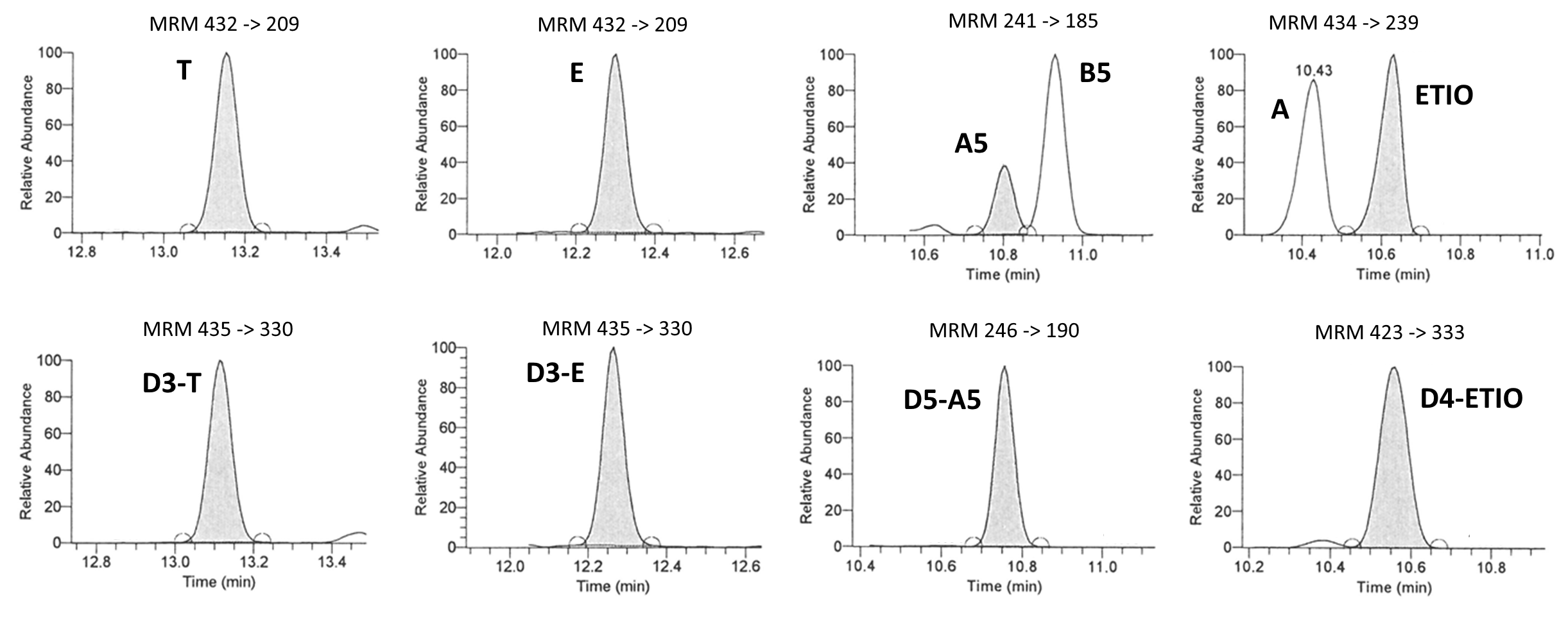
Figure 2: Extracted chromatograms obtained for an unsuspicious urine sample. Shown are the multiple reaction monitoring (MRM) ion transitions employed for the quantification of endogenous steroids (upper part) and their deuterated analogues (lower part).

A total of 1433 normal urine samples were obtained from 100 athletes (50 males and 50 females), 2504 samples were obtained from 100 athletes (50 males and 50 females) whose longitudinal steroid profiles contain values classified as atypical, and 462 samples from 29 athletes (15 males and 14 females) with at least one confirmed abnormal value in their steroid profile, employing IRMS in line with WADA regulation [21]. Figure A.1 in Appendix A shows that there is severe imbalance between normal (grey) and non-normal (black) samples with the former specifying the majority class. Specifically, out of 4399 urine samples across all athletes, only 327 (7.43%) were non-normal values (275 from athletes with atypical samples, and 52 from athletes with abnormal samples). Sample calibration was carried out prior to the analysis according to the estimated real limits of the applied methodology. Limit of detection (LOD) values and limit of quantification (LOQ) values within the steroid profiles of the athletes have been replaced by commonly accepted minimum cut-off values for all markers; i.e. all $<$LOQ and $<$LOD values in testosterone and epitestosterone were replaced by 1 ng/mL and 0.1 ng/mL respectively, while for $<$LOQ and $<$LOD values in the -diols were replaced by 5 ng/mL and 1 ng/mL, respectively.

Furthermore, single EAAS and ratio measurements of 164 healthy individuals have been provided as part of a cross-sectional study, representing a baseline population of which 91 were men and 73 women of age between 18 and 54 [19]. Figure A.2 in Appendix A presents the scatter and density plots for men (black) and women (grey) for all available markers and ratios. The concentrations of markers seem to be slightly separable between men and women. However, this does not apply to the ratios, where the distributions of both sexes seem similar, except for the A/T ratio. The correlation between the various markers and ratios shows that plain markers are more highly correlated compared to the ratios (Figure A.2). Tables B.2, B.3, B.4 and B.5 summarise the statistics (minimum, 1st quartile; Q1 and 3rd quartile; Q3, mean, median, maximum EAAS values and standard deviation) of the baseline population and the longitudinally-monitored athletes. The boxplots of the mean values of the available longitudinal metabolites and ratios are reported in Figure 3. When available, the WADA limits (lower and/or upper) are denoted by the solid lines based on Table B.6. Androsterone and Etiocholanolone share the same population thresholds among females and males. When population-specific information is unavailable for certain ratios, the Q3 values derived from the cross-sectional dataset are used as initial population thresholds for the respective ratios.

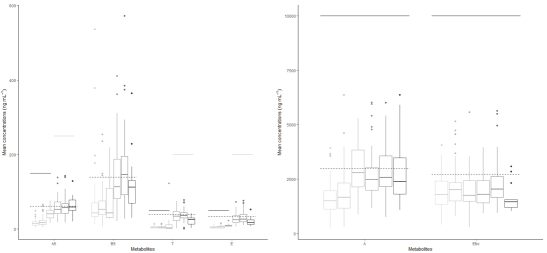
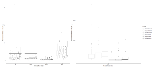
Figure 3: Boxplots for the mean values of the metabolite concentrations (ng mL^-1) and their ratios from 229 athletes by sex and doping status (normal, atypical and abnormal). WADA limits are denoted by the solid lines. Dashed lines represent the mean concentrations of the metabolites obtained from the baseline population.

4.2 Estimation of highest posterior predictive density

4.2.1 Univariate HPD estimation

To implement the univariate Bayesian model for each athlete and each biomarker in the ABP separately, we initially specified the prior distributions for the model parameters as described in Equations (2) and (3). While the correlation between the empirical mean and precision of log-transformed concentration values across all markers was relatively weak, ranging from -0.33 to 0.32, we consider a prior dependency between the parameters $\mu$ and $\tau$. We set the hyperparameters $\kappa_{0}=1$, $\alpha_{0}=10$, and $\beta_{0}=1$, while we control for possible confounding due to sex differences by setting $\mu_{0}=\mu_{js}$, that is the mean of the $j$th marker in its logarithmic scale for male subjects if $s=0$, and for females if $s=1$, obtained from the baseline cross-sectional dataset. After the burn-in period of 1000 draws, 5000 draws for each parameter were sampled from the known joint posterior distribution (Gaussian-Gamma). The out-of-sample predictive distribution of a new test result $y_{n+1}$ given the previous recordings $\boldsymbol{y}=(y_{1},y_{2},...,y_{n})$ is computed as

$$p(y_{n+1}|\boldsymbol{y})=\int\int p(y_{n+1}|\mu,\tau)p(\mu,\tau|\boldsymbol{y})d\mu d\tau\approx\frac{1}{T}\sum_{t=1}^{T}\bigg{(}\frac{\tau^{(t)}}{2\pi}\bigg{)}^{1/2}e^{-\frac{\tau^{(t)}}{2}(y_{n+1}-\mu^{(t)})^{2}},$$ (10)

where $n\geq 0$, and $(\mu^{(t)},\tau^{(t)})$ is the parameter pair of the $t$th draw obtained through the sampler with total number of iterations $T=5000$. In practice, the integration averaging is performed using an empirical average based on samples from the posterior distribution. At first, we simulate replicates of new data, $y_{n+1}$, from the posterior predictive distribution and then we derive the $95\%$ HPD interval. Since the true class for each of the 4399 EAAS concentrations of the 229 athletes is known, we can estimate the predictive accuracy of the method.

In Figure 4, the A5 and T/E series of a doped athlete are depicted with the blue-solid lines. The red dotted lines are the 95% HPD intervals of the predictive distribution, which serve as the posterior normal boundaries at each specific time point. Before observing any data, the upper limits are defined by WADA’s population thresholds, when they are available (see Table B.6). For marker B5, we used the maximum value obtained by the Caucasian population in Van Renterghem et al. [16], while for the remaining ratios (A5/B5, A5/E and A/T) we chose the Q3 values 4, 10 and 10,000, respectively, as reasonable starting thresholds derived from the cross-sectional dataset. The purple dashed lines indicate the usual Z-score upper limits as presented in Sottas et al. [17]. The gold diamonds symbolise the abnormal values in the athlete’s profile, which the model considers as suspicious values that need further investigation. For the T/E ratio in Figure 4(b), there are two additional green dashed-dotted lines that indicate the upper and lower limits of the T/E model with informative priors introduced by Sottas et al. [17]. For example, in Figure 4(a), there are two androsterone samples which are higher than the upper limits, and in Figure 4(b), Sottas’ model identifies four abnormal T/E tests, out of which three are in common with those suggested by the general univariate model.

Figure 4: A series of 29 longitudinal values of (a) A5 and (b) T/E (blue solid-dotted line) obtained from a doped athlete; the upper and lower limits (red dotted lines) are the 95% HPD intervals from the univariate Bayesian model; upper limits based on a usual Z-score (purple dashed line); abnormal values are marked with gold diamonds. For (b), upper and lower limits (green dashed-dotted lines) are the 95% HPD interval from the T/E model of Sottas et al. [17], with its suggested abnormal values indicated by green stars.

Figure A.3 (a-k) displays the series of the six EAAS along with their five corresponding ratios for the same athlete. Given that the 21^st, 22^nd and 23^rd sample tests of that athlete are confirmed as abnormal, only E, T/E and A5/E were sensitive enough to detect these anomalies within the athlete’s steroid profile. Note that if the model suggests a sample as an outlier, we automatically exclude it from the set of recordings which are used to compute the HPD intervals, because it might have an impact on the validity of the following personalised normal limits.

4.2.2 Multivariate HPD estimation

To apply the multivariate Bayesian adaptive model, we initially specified the prior distributions for the model parameters $\boldsymbol{\theta}=(\boldsymbol{\mu},\{\boldsymbol{\mu_{j}}\}_{j=1}^{J},\Omega_{e},\Omega_{\mu},\Omega_{b})$ as described in Section 2.2. The prior covariance matrices $S_{e}$, $S_{\mu}$ and $S_{b}$ are all set equal to $(1/1000)\mathbb{I_{K}}$, and the degrees of freedom are $d_{e}=d_{\mu}=d_{b}=K-1$, where $K$ is the dimensionality of the data. We use historical prior information obtained from the baseline cross-sectional dataset of 164 non-doped athletes (91 men and 73 women), which is captured by the prior mean vector $\boldsymbol{\mu_{0}}$. Similarly, as in the univariate case, the model can accommodate distinct prior mean vectors for both men and women. Then, $3000$ draws were sampled for each parameter from the posterior distribution $p(\boldsymbol{\theta}|\boldsymbol{y})$ using the Gibbs sampler, while the first $1/3$ was discarded. Given the remaining set of samples $\{\boldsymbol{\theta^{(t)}}\}_{t=1}^{T=2000}$, our estimate for the predictive distribution is

$$p(\boldsymbol{y_{n+1}}|\boldsymbol{y})\approx\frac{1}{T}\sum_{t=1}^{T}(2\pi)^{-K/2}|\Omega_{e}^{(t)}|^{-1/2}\exp\left(-\frac{1}{2}(\boldsymbol{y_{n+1}}-\boldsymbol{\mu_{j}^{(t)}})^{T}\Omega_{e}^{(t)}(\boldsymbol{y_{n+1}}-\boldsymbol{\mu_{j}^{(t)}})\right)$$ (11)

We first simulate from the posterior predictive distribution many replicates of the new data, $\boldsymbol{y_{n+1}}$, and thus we derive the 95% HPD interval. Data from athletes with exclusively normal samples were used for model training, whereas atypical and abnormal samples comprised the test set. The idea is to train the model with normal data from non-doped athletes, by estimating $p(\boldsymbol{\theta}_{\text{normal}}|\boldsymbol{y_{\text{normal}}})$ and then test how likely it is for a future unlabelled observation to be generated by this model.

4.3 Classification performance

In forensic toxicology, high specificity is important, thus a very low false positive rate is required in order to prevent the accusation of an innocent athlete. However, classification accuracy values and measures regarding the majority class such as the overall accuracy, tend to be pretty high because they are computed under the assumption of balanced class distributions. Consequently, we need to use appropriate metrics for evaluating the classification performance of the models which can deal with the imbalance of the dataset, such as the F1 score and G-mean (Geometric mean) defined as

$$F1\text{-score}=\frac{2\times\text{Precision}\times\text{Recall}}{\text{Precision}+\text{Recall}},$$ (12)

and

$$G\text{-mean}=\sqrt{\text{Sensitivity}\times\text{Specificity}}$$ (13)

Table 1 presents the classification performance of the univariate model and the MBA model (before and after oversampling), in comparison with the univariate T/E model proposed by Sottas et al. [17], the univariate Euclidean distance (ED) score model of de Figueiredo et al. [23] and a generalised linear mixed-effects model (GLMM) using a false positive rate $\alpha=0.05$. The GLMM model is implemented via the glmer() function in R to fit a mixed effects logistic regression model with a binomial distribution for the response variable “Class_ij”, which is a binary response variable that represents the class of each observation $i$ of athlete $j$ including the biomarkers and/or ratios as individual level continuous predictors, and a random intercept by athlete ID. The classification using the univariate models suggest the T/E, A/ETIO and A5/E ratios as the most sensitive variables for detecting anomalies in the steroidal profile with higher $F1$ scores ($F1_{{T/E}^{1}}=0.19$, $F1_{A/ETIO}=0.24$ and $F1_{A5/E}=0.23$). Regarding the T/E models, the one employing informative priors demonstrates slightly better predictive performance in contrast to the model using semi-informative conjugate priors, as indicated by the improved metrics $F1_{{T/E}^{2}}=0.20$, sensitivity${}_{{T/E}^{2}}=0.32$ and balanced accuracy${}_{{T/E}^{2}}=0.59$.

In Figure 5, we have also presented the ROC (Receiver Operating Characteristic) curves and the Precision-Recall curves to measure the accuracy of the classification predictions in the various models. According to the ROC curves, the model for the A5/E ratio showed superiority compared to the other univariate models in Figure 5(a), while the model for A/ETIO ratio showed superiority in the Precision-Recall plot. However, the superior performance of the A/ETIO ratio was unexpected based on the current literature, which is an aspect that warrants further investigaton. The curve using the model of Sottas et al. [17] for T/E is higher in Figure 5(b), which verifies its higher predictive performance.

Classification							Balanced	Overall
model	Variable	$G$-mean	$F_{1}$	Precision	Sensitivity	Specificity	Accuracy	Accuracy (95% CI)
Univariate	A5	0.46	0.15	0.11	0.25	0.84	0.55	0.80 (0.79, 0.81)
	B5	0.50	0.17	0.12	0.30	0.83	0.56	0.79 (0.78, 0.80)
	A	0.38	0.13	0.11	0.17	0.86	0.53	0.83 (0.82, 0.84)
	ETIO	0.38	0.12	0.10	0.16	0.89	0.52	0.84 (0.82, 0.85)
	T	0.50	0.18	0.13	0.30	0.83	0.57	0.79 (0.78, 0.81)
	E	0.52	0.17	0.11	0.34	0.78	0.56	0.75 (0.73, 0.76)
	T/E1	0.48	0.19	0.15	0.26	0.88	0.57	0.84 (0.82, 0.85)
	A/ETIO	0.41	0.24	0.39	0.17	0.98	0.58	0.92 (0.91, 0.93)
	A/T	0.39	0.15	0.13	0.17	0.91	0.54	0.86 (0.85, 0.87)
	A5/B5	0.47	0.18	0.14	0.25	0.88	0.57	0.84 (0.82, 0.85)
	A5/E	0.55	0.23	0.17	0.35	0.86	0.61	0.82 (0.81, 0.83)
Sottas et al. [17]	T/E2	0.52	0.20	0.15	0.32	0.85	0.59	0.81 (0.80, 0.82)
pre-oversampling	EAAS	0.55	0.24	0.18	0.38	0.78	0.58	0.74 (0.72, 0.75)
MBA	ratios	0.62	0.35	0.29	0.44	0.87	0.65	0.82 (0.80, 0.83)
	all	0.63	0.30	0.20	0.55	0.73	0.64	0.71 (0.70, 0.73)
post-oversampling	EAAS	0.49	0.44	0.50	0.39	0.61	0.50	0.50 (0.49, 0.51)
MBA	ratios	0.46	0.38	0.50	0.31	0.69	0.50	0.50 (0.48, 0.52)
	all	0.50	0.49	0.50	0.47	0.53	0.50	0.50 (0.49, 0.52)
pre-oversampling	EAAS	0.22	0.20	0.11	0.98	0.05	0.52	0.15 (0.14, 0.17)
univariate	ratios	0.22	0.20	0.11	0.99	0.05	0.52	0.15 (0.14, 0.16)
ED score	all	0.20	0.20	0.11	0.99	0.04	0.52	0.15 (0.14, 0.16)
post-oversampling	EAAS	0.17	0.66	0.50	0.97	0.03	0.50	0.50 (0.49, 0.51)
univariate	ratios	0.14	0.66	0.50	0.98	0.02	0.50	0.50 (0.49, 0.51)
ED score	all	0.14	0.66	0.50	0.98	0.02	0.50	0.50 (0.49, 0.51)
pre-oversampling	EAAS	0.10	0.02	1	0.01	1	0.51	0.88 (0.87, 0.90)
GLMM	ratios	0.25	0.11	0.82	0.06	1	0.53	0.89 (0.87, 0.90)
	all	0.25	0.12	0.83	0.06	1	0.53	0.89 (0.87, 0.90)
post-oversampling	EAAS	0.20	0.08	0.79	0.04	0.99	0.51	0.51 (0.49, 0.53)
GLMM	ratios	0.38	0.26	0.89	0.15	0.98	0.57	0.57 (0.55, 0.59)
	all	0.39	0.27	0.81	0.16	0.96	0.56	0.56 (0.54, 0.58)

• This model specifies weakly informative priors.

• For Sottas’ model the priors are set to be strongly informative.

Table 1: Predictive performance of the univariate and multivariate models on the athletes’ profiles based on the 95% HPD interval.

The proposed multivariate Bayesian adaptive model (MBA) has been applied to: a) EAAS markers only; b) ratios only; and c) all EAAS markers and ratios; using both the original dataset and the dataset after over-sampling. The $G$-mean and $F1$ metrics for the MBA models, as shown in Table 1 before oversampling, exhibit consistently higher values when compared to their counterparts in the univariate models. Comparing further between the performance of the MBAs, the five available ratios were found to be the most powerful set of variables before oversampling with the highest metric values $F1_{MBA_{ratios}}=0.35$, precision${}_{MBA_{ratios}}=0.29$, sensitivity${}_{MBA_{ratios}}=0.44$, specificity${}_{MBA_{ratios}}=0.87$ and highest balanced accuracy${}_{MBA_{ratios}}=0.65$. While the $G$-mean value for the model applied to the five ratios ($G\text{-mean}_{MBA_{ratios}}=0.62$), is slightly lower that of the model applied to the six markers and five ratios ($G\text{-mean}_{MBA_{all}}=0.63$), it is important to note that the model focusing on the ratios remains equally powerful despite utilizing less information. Similar conclusions about the superiority of the pre-oversampling multivariate model, assessed through the use of ratios, can be derived from an examination of the plots in Figure 5(c). Here, the blue lines point to a better relationship between sensitivity and 1-specificity, as well as between precision and recall.

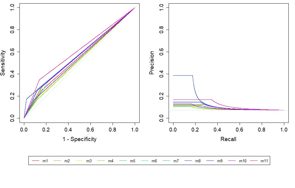
(a)

(b)

(c)

Figure 5: ROC curves obtained from (a) the univariate models (m1: A5, m2: B5, m3: A, m4: ETIO, m5: T, m6: E, m7: T/E, m8: A/ETIO, m9: A/T, m10: A5/B5, m11: A5/E), (b) m1: T/E model vs m2: Sottas’ model for T/E, and (c) the multivariate models (m1: all EAAS markers and ratios, m2: EAAS only, m3: ratios only) applied to the original dataset.

In Figure 6, all classification metrics are plotted for the applied models. Once more, the conclusion is clear that the multivariate Bayesian adaptive model (MBA) before oversampling applied solely to the ratios, consistently delivers the best overall classification performance ($F1_{MBA_{ratios}}=0.25$ and $G$-mean${}_{MBA_{ratios}}=0.62$) compared to the univariate models, the univariate ED score models and the GLMMs. The problem of unreliable overall accuracy in imbalanced data has been alleviated through the application of oversampling techniques, as evidenced by the now equivalent values of balanced accuracy and overall accuracy (see Table 1). Comparing the $F1$ scores before and after oversampling, it appears that applying the random oversampling method enhances the overall classification performance of the models. It is noteworthy that the univariate ED score model exhibits considerably higher sensitivity and lower specificity values, indicating a tendency to classify normal values as abnormal. Conversely, the GLMM performance is characterised by significantly higher specificity and lower sensitivity values, suggesting a propensity to classify abnormal values as normal. Therefore, their $F1$ score values are biased towards either very high or very low sensitivity. To address this, we employ the $G$-mean metric to compare all models after oversampling, which is the harmonic mean of sensitivity and specificity as defined in 13. After oversampling, the highest $G$-mean values are consistently achieved by the multivariate Bayesian adaptive model, which outperforms the univariate ED score model and GLMM.

Figure 6: Classification metrics per component; i.e. markers and ratios separately, only EAAS, only ratios, all EAAS markers and ratios. T/E₁ corresponds to the T/E model from Section 2.1, while T/E₂ corresponds to the T/E model by Sottas et al. [17]. Subscripts “pre”, “post”, denote pre-oversampling and post-oversampling, respectively.

5 Discussion

Our primary objective in this research was to develop a multivariate Bayesian adaptive model for repeated measurements of various urinary biomarkers and their ratios, as a generalisation of a widely used univariate model [17] which also uses urinary steroid profile data for doping detection. Similar to the univariate model, the proposed methodology considers the population distribution of these biomarkers and the individual’s own history; i.e. previous measurements of the athlete’s biomarkers. In addition, it has the capacity to incorporate other relevant demographic characteristics such as the athlete’s sex or age. The method simultaneously models multiple measurements of endogenous substances that are able to reveal the presence of doping agents, and utilises a one-class classification rule to improve detection performance in the presence of class imbalance. The resulting personalised normal ranges for athletes’ longitudinal steroid profiles show improved detection performance in a dataset of professional athletes, as compared to the performance of the existing univariate model. The proposed method thus appears promising as an additional monitoring tool in the anti-doping toolkit. One of the method’s advantages is that it relies on the urinary steroid profile, which produces easily accessible, reliable, quickly quantifiable and reproducible data from samples that are obtained in a non-invasive way and with a low financial cost. In addition, an implementation of this model is available as a user-friendly software designed specifically for anti-doping laboratories.

A challenging aspect of this work was the presence of class imbalance due to the scarcity of data from confirmed doping cases. Oversampling was utilised to alleviate this problem, although other techniques such as undersampling, a combination of undersampling and oversampling or boosting algorithms that are able to convert weak learners to strong learners [34, 36] could also be explored. Applications on additional markers and ratios is another direction which is worth investigating. An illustrative example of this concept can be found in the work of Wilkes et al. [37]. Lastly, this research examines the predictive performance of the Bayesian adaptive model when applied to six biomarkers and five ratios. It would be of interest to explore whether a subset of these variables could further improve performance. Further testing on additional datasets is needed to produce robust recommendations as to the optimal implementation of the model.

Appendix A Figures

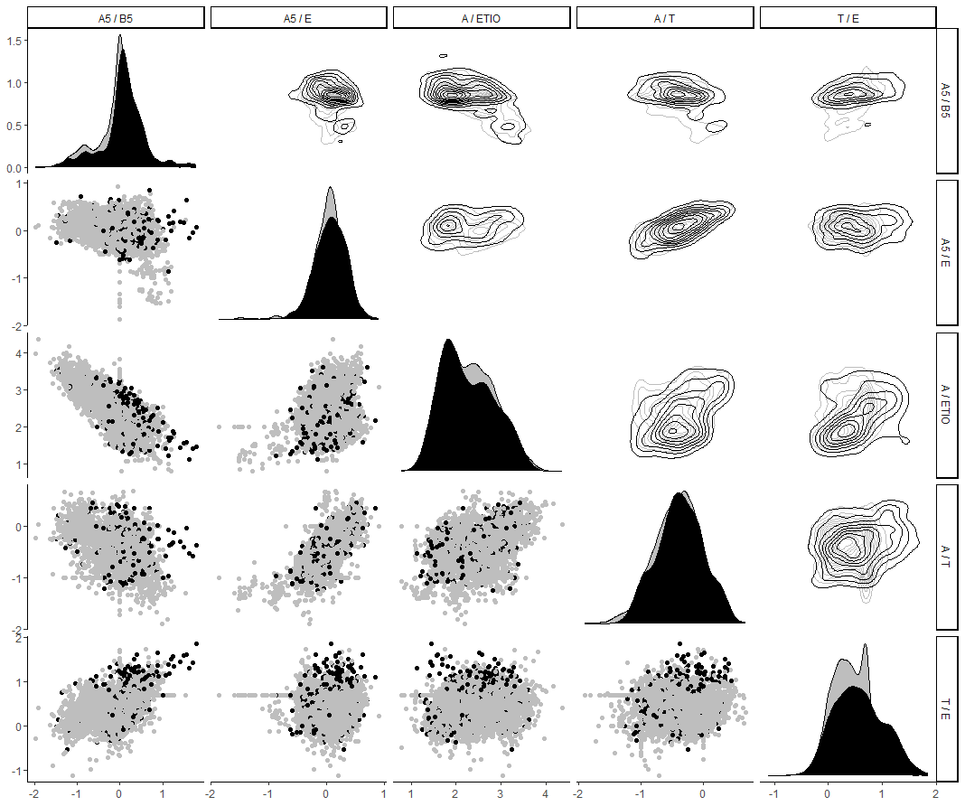
Figure A.1: Plots of normal (grey) vs non-normal (black) samples including the scatter, density and contour plots for (a) the six markers, and (b) their five ratios in the logarithmic scale.

Figure A.2: Scatter and density plots by sex accompanied by the correlation coefficients for (a) the six markers, and (b) their five ratios in the logarithmic scale.

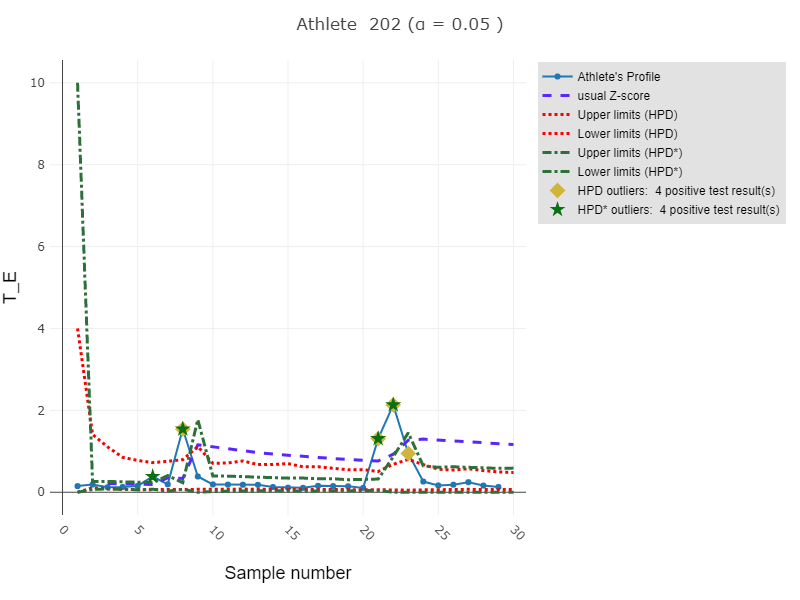
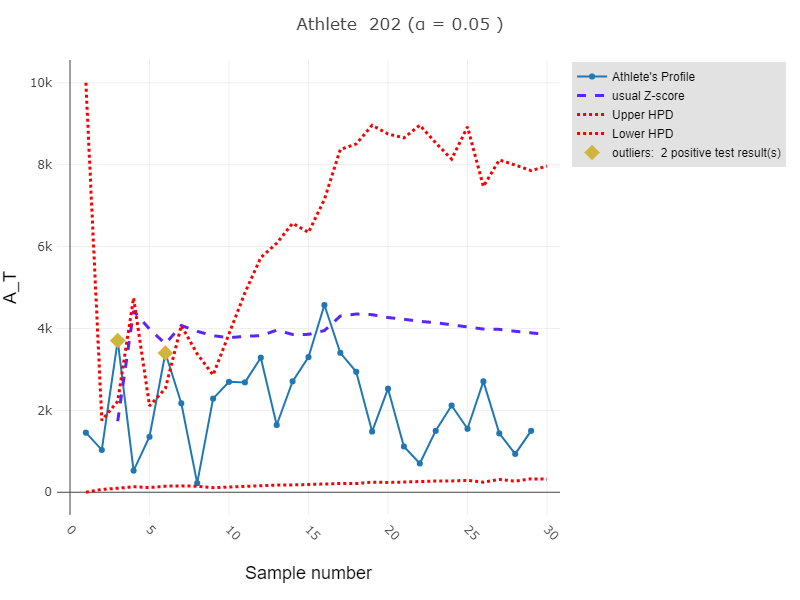
Figure A.3: (a-k) A series of 29 longitudinal values of the six EAAS and their five ratios (blue solid-dotted line) obtained from a doped athlete; upper and lower limits (red dotted lines) are calculated using the 95% HPD intervals of the predictive distribution from the univariate Bayesian model; upper limits assuming a usual Z-score (purple dashed line); suggested abnormal values are denoted by the gold diamonds. (g) Upper and lower limits (green dashed-dotted lines) are calculated using the 95% HPD interval of the predictive distribution from the T/E model of Sottas et al. [17]; suggested abnormal values based on the T/E model are denoted by the green stars.

Appendix B Tables

Trivial name	Abbreviation	Systematic name	Formula
5$\alpha$-Adiol	A5	5$\alpha$-Androstane-3$\alpha$,17$\beta$-diol	$C_{19}H_{32}O_{2}$
5$\beta$-Adiol	B5	5$\beta$-Androstane-3$\alpha$,17$\beta$-diol	$C_{19}H_{32}O_{2}$
Androsterone	A	3$\alpha$-Hydroxy-5$\alpha$-androstan-17-one	$C_{19}H_{30}O_{2}$
Epitestosterone	E	17$\alpha$-Hydroxy-androst-4-en-3-one	$C_{19}H_{28}O_{2}$
Etiocholanolone	ETIO	3$\alpha$-Hydroxy-5$\beta$-androstan-17-one	$C_{19}H_{30}O_{2}$
Testosterone	T	17$\beta$-Hydroxy-androst-4-en-3-one	$C_{19}H_{28}O_{2}$
5$\alpha$-Adiol/5$\beta$-Adiol	A5/B5
5$\alpha$-Adiol/Epitestosterone	A5/E
Androsterone/Etiocholanolone	A/ETIO
Androsterone/Testosterone	A/T
Testosterone/Epitestosterone	T/E

Table B.1: Urinary steroid metabolites quantitated in this study.

Target Metabolite	Min	Q1	Mean	Median	Q3	Max	SD
	(ng/mL)	(ng/mL)	(ng/mL)	(ng/mL)	(ng/mL)	(ng/mL)	(ng/mL)
A5	$1.46$	14.49	$61.7$	$46.62$	84.56	$388.14$	$64.68$
B5	$1.88$	40.46	$139.92$	$89.14$	180.92	$1,232.95$	$164.27$
A	$187.7$	1,315.9	$2,997.3$	$2,517.2$	4,428.1	$16,674.1$	$2,169.41$
E	$0.47$	4.31	$33.71$	$20.52$	42.22	$252.96$	$42.94$
ETIO	$187.5$	1,379.8	$2,719.4$	$2,337.9$	3,614	$9,819.9$	$1,803.23$
T	$0.14$	4.17	$39.37$	$20.39$	61.43	$229.03$	$46.27$
A5/B5	$0.03$	0.3	$0.64$	$0.46$	0.74	$15.57$	$1.22$
A5/E	$0.24$	1.47	$3.29$	$2.73$	4.23	$17.72$	$2.54$
A/ETIO	$0.17$	0.78	$1.17$	$1.05$	1.47	$3$	$0.53$
A/T	$13.13$	53.97	$374.49$	$125.08$	282.92	$14,154.24$	$1,269.35$
T/E	$0.01$	0.76	$1.63$	$1.44$	2.19	$6.48$	$1.16$

Table B.2: Descriptive summaries (minimum, 1st quartile; Q1, mean, median, 3rd quartile; Q3, maximum and standard deviation (SD)) of the metabolites and ratios of the baseline healthy population (91 men and 73 women).

	Min	Q1	Mean	Median	Q3	Max
Target Metabolite	(ng/mL)	(ng/mL)	(ng/mL)	(ng/mL)	(ng/mL)	(ng/mL)
A5	$1$	11	$35.08$	25	$49$	210
B5	$1$	34	$96.25$	$64$	120	$910$
A	$100$	1,200	$2,097$	$1,800$	2,600	$16,000$
E	$0.10$	4	$17.48$	$11$	26	$130$
ETIO	$98$	1,100	$1,863$	$1,700$	2,400	$7,200$
T	$0.10$	3.30	$20.17$	$9.60$	31	$150$
A5/B5	$0.013$	0.24	$0.49$	$0.40$	0.61	$4.8$
A5/E	$0.13$	1.41	$4.77$	$2.54$	4.65	$160$
A/ETIO	$0.06$	0.80	$1.21$	$1.11$	1.48	$8.16$
A/T	$6.25$	72.41	$365.25$	$159.46$	412.7	$23,000$
T/E	$0.012$	0.75	$1.35$	$1.0$	1.6	$13$

Table B.3: Descriptive summaries (minimum, 1st quartile; Q1, mean, median, 3rd quartile; Q3, and maximum) of the metabolites and ratios of 100 athletes with normal samples.

	Min	Q1	Mean	Median	Q3	Max
Target Metabolite	(ng/mL)	(ng/mL)	(ng/mL)	(ng/mL)	(ng/mL)	(ng/mL)
A5	$1.0$	14	$36.61$	28.0	$50$	250
B5	$3.3$	43	105.1	$73$	140	$1,400$
A	$100$	1,200	2,318	$2,000$	3,000	$13,000$
E	$0.10$	4.50	18.53	$12.0$	27	$160$
ETIO	$270$	1,300	2,199	$1,900$	2,700	$14,000$
T	$0.10$	3.3	19.44	$9.25$	33	$150$
A5/B5	$0.02$	0.19	$0.48$	$0.35$	0.65	$4.6$
A5/E	$0.08$	1.42	$3.38$	$2.37$	4.6	$53.33$
A/ETIO	$0.014$	0.7	$1.16$	$1.04$	1.46	$6.91$
A/T	$6.252$	67.66	$454.63$	$183.33$	525.65	$9,200$
T/E	$0.01$	0.62	1.46	$1$	1.64	$35$

Table B.4: Descriptive summaries (minimum, 1st quartile; Q1, mean, median, 3rd quartile; Q3, and maximum) of the metabolites and ratios of 100 athletes with atypical samples.

	Min	Q1	Mean	Median	Q3	Max
Target Metabolite	(ng/mL)	(ng/mL)	(ng/mL)	(ng/mL)	(ng/mL)	(ng/mL)
A5	$3.7$	21	$50.53$	39.5	$65$	270
B5	$4.9$	24	$82.69$	$50$	97	$2,200$
A	$210$	1,600	$3,152$	$2,400$	3,900	$16,000$
E	$1$	5.90	$14.41$	$11$	19	$120$
ETIO	$100$	932.5	$1,747$	$1,500$	2,175	$11,000$
T	$0.50$	1	$12.51$	$3.50$	15	$220$
A5/B5	$0.085$	0.47	$0.76$	$1$	1.42	$4.2$
A5/E	$0.46$	1.83	$5.59$	$3.55$	5.91	$72.22$
A/ETIO	$0.50$	1.17	$1.92$	$1.69$	2.53	$5.08$
A/T	$13.18$	177.55	$1,262.99$	$632.46$	1,800	$14,828$
T/E	$0.03$	0.15	$1.58$	$0.34$	1.3	$61.11$

Table B.5: Descriptive summaries (minimum, 1st quartile; Q1, mean, median, 3rd quartile; Q3, and maximum) of the metabolites and ratios of 29 athletes with abnormal samples.

Target Metabolite	Max (M)	Max (F)	WADA TD 2021 (M)	WADA TD 2021 (F)
	(ng/mL)	(ng/mL)	(ng/mL)	(ng/mL)
A5	652	263	250	150
B5	1,260	471
A	20,700	17,500	10,000	10,000
E	391	51.9	200	50
ETIO	11,400	9,030	10,000	10,000
T	249	219	200	50
A/ETIO			4	4
T/E			4	4
Target Metabolite	IUL (M)	IUL (F)
	(ng/mL)	(ng/mL)
A5/B5	4	4
A5/E	10	10
A/T	10000	10000

Table B.6: Maximum EAAS values and their ratios measured in a Caucasian population consisting of 2,027 male (M) and 1,004 female (F) athletes [16] along with the available WADA’s threshold limits by sex [38, 7]. The initial upper limits (IUL) for ratios, in cases where there is no available population-specific information, are determined from the upper limit of the inter-quartile range (Q3) observed in the corresponding ratios within the cross-sectional dataset.

References

- Kanayama and Pope Jr [2018] Gen Kanayama and Harrison G Pope Jr. History and epidemiology of anabolic androgens in athletes and non-athletes. Molecular and Cellular Endocrinology, 464:4–13, 2018.
- [2] World Anti-Doping Agency (WADA). 2019 anti-doping testing figures samples analyzed and reported by accredited laboratories in adams, 2019.
- Sottas et al. [2010] Pierre-Edouard Sottas, Martial Saugy, and Christophe Saudan. Endogenous steroid profiling in the athlete biological passport. Endocrinology and Metabolism Clinics, 39(1):59–73, 2010.
- [4] World Anti-Doping Agency (WADA). Technical document - td2021eaas: Measurement and reporting of endogenous anabolic androgenic steroid (eaas) markers of the urinary steroid profile, 2021a.
- Sottas et al. [2011] Pierre-Edouard Sottas, Neil Robinson, Olivier Rabin, and Martial Saugy. The athlete biological passport. Clinical chemistry, 57(7):969–976, 2011.
- Vernec [2014] Alan R Vernec. The athlete biological passport: an integral element of innovative strategies in antidoping. British journal of sports medicine, 48(10):817–819, 2014.
- [7] World Anti-Doping Agency (WADA). Wada technical document – td2021apmu, 2021b.
- Kuuranne et al. [2014] Tiia Kuuranne, Martial Saugy, and Norbert Baume. Confounding factors and genetic polymorphism in the evaluation of individual steroid profiling. British journal of sports medicine, 48(10):848–855, 2014.
- Piper et al. [2021] Thomas Piper, Hans Geyer, Nadine Haenelt, Frank Huelsemann, Wilhelm Schaenzer, and Mario Thevis. Current insights into the steroidal module of the athlete biological passport. International Journal of Sports Medicine, 2021.
- Mareck et al. [2008] Ute Mareck, Hans Geyer, Georg Opfermann, Mario Thevis, and Wilhelm Schänzer. Factors influencing the steroid profile in doping control analysis. Journal of Mass Spectrometry, 43(7):877–891, 2008.
- Harris [1974] Eugene K Harris. Effects of intra-and interindividual variation on the appropriate use of normal ranges. Clinical Chemistry, 20(12):1535–1542, 1974.
- Brooks et al. [1979] R-V Brooks, G Jeremiah, Wendy A Webb, and M Wheeler. Detection of anabolic steroid administration to athletes. Journal of steroid biochemistry, 11(1):913–917, 1979.
- Donike et al. [1983] M Donike, KR Barwald, K Klostermann, W Schanzer, and J Zimmermann. Nachweis von exogenem testosteron [detection of exogenous testosterone], 1983.
- Sottas et al. [2006] Pierre-Edouard Sottas, Neil Robinson, Sylvain Giraud, Franco Taroni, Matthias Kamber, Patrice Mangin, and Martial Saugy. Statistical classification of abnormal blood profiles in athletes. The International Journal of Biostatistics, 2(1), 2006.
- Sottas et al. [2008] Pierre-Edouard Sottas, Christophe Saudan, Carine Schweizer, Norbert Baume, Patrice Mangin, and Martial Saugy. From population-to subject-based limits of t/e ratio to detect testosterone abuse in elite sports. Forensic science international, 174(2-3):166–172, 2008.
- Van Renterghem et al. [2010] Pieter Van Renterghem, Peter Van Eenoo, Hans Geyer, Wilhelm Schänzer, and Frans T Delbeke. Reference ranges for urinary concentrations and ratios of endogenous steroids, which can be used as markers for steroid misuse, in a caucasian population of athletes. Steroids, 75(2):154–163, 2010.
- Sottas et al. [2007] Pierre-Edouard Sottas, Norbert Baume, Christophe Saudan, Carine Schweizer, Matthias Kamber, and Martial Saugy. Bayesian detection of abnormal values in longitudinal biomarkers with an application to t/e ratio. Biostatistics, 8(2):285–296, 2007.
- Brown et al. [2001] Philip J Brown, Michael G Kenward, and Eryl E Bassett. Bayesian discrimination with longitudinal data. Biostatistics, 2(4):417–432, 2001.
- Alladio et al. [2016] Eugenio Alladio, Roberto Caruso, Enrico Gerace, Eleonora Amante, Alberto Salomone, and Marco Vincenti. Application of multivariate statistics to the steroidal module of the athlete biological passport: a proof of concept study. Analytica chimica acta, 922:19–29, 2016.
- Amante et al. [2019] Eleonora Amante, Serena Pruner, Eugenio Alladio, Alberto Salomone, Marco Vincenti, and Rasmus Bro. Multivariate interpretation of the urinary steroid profile and training-induced modifications. the case study of a marathon runner. Drug testing and analysis, 11(10):1556–1565, 2019.
- [21] World Anti-Doping Agency (WADA). Wada technical document – td2021irms, 2021c.
- [22] The R Project for Statistical Computing. URL https://www.r-project.org/. Accessed: October 20, 2023.
- de Figueiredo et al. [2023] Miguel de Figueiredo, Jonas Saugy, Martial Saugy, Raphaël Faiss, Olivier Salamin, Raul Nicoli, Tiia Kuuranne, Serge Rudaz, Francesco Botrè, and Julien Boccard. A new multimodal paradigm for biomarkers longitudinal monitoring: a clinical application to women steroid profiles in urine and blood. Analytica Chimica Acta, 1267:341389, 2023.
- Eleftheriou [2022] Dimitra Eleftheriou. Bayesian hierarchical modelling for biomarkers with applications to doping detection and prostate cancer prediction. PhD thesis, University of Glasgow, 2022.
- DeGroot [2005] Morris H DeGroot. Optimal statistical decisions, volume 82. John Wiley & Sons, 2005.
- Casella and George [1992] George Casella and Edward I George. Explaining the Gibbs sampler. The American Statistician, 46(3):167–174, 1992.
- Gelman et al. [2013] Andrew Gelman, John B Carlin, Hal S Stern, David B Dunson, Aki Vehtari, and Donald B Rubin. Bayesian data analysis. CRC press, 2013.
- Minter [1975] TC Minter. Single-class classification. In LARS Symposia, page 54, 1975.
- Bishop [1994] Christopher M Bishop. Novelty detection and neural network validation. IEE Proceedings-Vision, Image and Signal processing, 141(4):217–222, 1994.
- Khan and Madden [2014] Shehroz S Khan and Michael G Madden. One-class classification: taxonomy of study and review of techniques. The Knowledge Engineering Review, 29(3):345–374, 2014.
- Hyndman [1996] Rob J Hyndman. Computing and graphing highest density regions. The American Statistician, 50(2):120–126, 1996.
- Rauth [1994] Susanne Rauth. Referenzbereiche von urinären Steroidkonzentrationen und Steroidquotienten: ein Beitrag zur Interpretation des Steroidprofils in der Routinedopinganalytik. PhD thesis, Deutsche Sporthochschule Köln, 1994.
- Kicman et al. [1995] Andrew T Kicman, Sarah B Coutts, Christopher J Walker, and David A Cowan. Proposed confirmatory procedure for detecting 5 alpha-dihydrotestosterone doping in male athletes. Clinical chemistry, 41(11):1617–1627, 1995.
- Kotsiantis et al. [2006] Sotiris Kotsiantis, Dimitris Kanellopoulos, Panayiotis Pintelas, et al. Handling imbalanced datasets: A review. GESTS International Transactions on Computer Science and Engineering, 30(1):25–36, 2006.
- Lunardon et al. [2014] Nicola Lunardon, Giovanna Menardi, and Nicola Torelli. ROSE: A Package for Binary Imbalanced Learning. R journal, 6(1), 2014.
- Schapire [2013] Robert E Schapire. Explaining adaboost. In Empirical inference, pages 37–52. Springer, 2013.
- Wilkes et al. [2018] Edmund H Wilkes, Gill Rumsby, and Gary M Woodward. Using machine learning to aid the interpretation of urine steroid profiles. Clinical chemistry, 64(11):1586–1595, 2018.
- [38] World Anti-Doping Agency (WADA). Wada technical document – td2018eaas: Endogenous anabolic androgenic steroids - measurement and reporting, 2018.