Instructions for *ACL Proceedings

Toward Stronger Textual Attack Detectors

Abstract

The landscape of available textual adversarial attacks keeps growing, posing severe threats and raising concerns regarding the deep NLP system’s integrity. However, the crucial problem of defending against malicious attacks has only drawn the attention in the NLP community. The latter is nonetheless instrumental in developing robust and trustworthy systems. This paper makes two important contributions in this line of search: (i) we introduce LAROUSSE, a new framework to detect textual adversarial attacks and (ii) we introduce STAKEOUT, a new benchmark composed of nine popular attack methods, three datasets, and two pre-trained models. LAROUSSE is ready-to-use in production as it is unsupervised, hyperparameter-free, and non-differentiable, protecting it against gradient-based methods. Our new benchmark STAKEOUT allows for a robust evaluation framework: we conduct extensive numerical experiments which demonstrate that LAROUSSE outperforms previous methods, and which allows to identify interesting factors of detection rate variations.

1 Introduction

Despite the high performances of deep learning techniques for Natural Language Processing (NLP) applications, the trained models remain vulnerable to adversarial attacks Barreno et al. (2006); Morris et al. (2020a) which limits their adoption for critical applications. In the context of NLP, for a given model and a given textual input, an adversarial example is a carefully constructed modification of the initial text such that it is semantically similar to the original text while affecting the model’s prediction. The ability to design adversarial examples Alves et al. (2018); Johnson (2018); Subbaswamy and Saria (2020) raises serious concerns regarding the security of NLP systems. It is, therefore, crucial to develop proper strategies that are available to deal with these threats Szegedy et al. (2014).

Perhaps surprisingly, if the research community has invested considerable efforts to design efficient attacks, there are only a few works that address the issue of preventing them. One can distinguish two lines of research: detection methods that aim at discriminating between regular input and attacks; and defense methods that try to correctly classify adversarial inputs. The latter is based on robust training methods, which customize the learning process, see for instance Zhou et al. (2021); Jones et al. (2020); Yoo and Qi (2021); Pruthi et al. (2019). These are limited to certain types of adversarial lures (e.g., misspelling), making them vulnerable to other types of attacks that already exist or may be designed in the future. In contrast, detection methods are more relevant to real-life scenarios where practitioners usually prefer to adopt a discard-rather-than-correct strategy Chow (1957). This has been highlighted in Yoo et al. (2022) which is, to the best of our knowledge, the single word that introduces a detection method that does not require training. On the contrary, the authors propose to measure the regularity of a given input by computing the Mahalanobis distance Mahalanobis (1936) of its embedding in the last layer of a transformer with respect to the training distribution. Notice that the Mahalanobis distance has also been successfully used in a very similar framework of Out-Of-Distribution (OOD) detection methods (see Lee et al. (2018); Ren et al. (2021) and references therein).

In this paper, we build upon Yoo et al. (2022) and introduce a new attack detection framework, called LAROUSSE, which improves the current state-of-the-art. Our approach is based on the computation of the halfspace-mass depth Chen et al. (2015); Picot et al. (2022a) of the last layer embedding of an input with respect to the training distribution. Halfspace-mass depth is a particular instance of data depth Darrin et al. (2023), which are functions that measure the proximity of a point to the core of a probability distribution. As a matter of fact, the Mahalanobis distance is also – probably one of the most popular – a data depth. Interestingly, in addition to improving the attack detection rate, the halfspace-mass depth remedies several limitations of the Mahalanobis depth: it does not make Gaussian assumptions on the data structure and is additionally non-differentiable, providing security guarantees regarding malicious adversaries that could rely on gradient-based methods.

The second contribution of our work consists in releasing STAKEOUT, a new NLP attack benchmark that enriches the one introduced in Yoo et al. (2022). More precisely, we explore the same datasets and extend their four attacks by adding five new adversarial techniques. This ensures a wider variety of testing methods, leading to a robust evaluation framework that we believe will stimulate future research efforts. We conduct extensive numerical experiments on STAKEOUT and demonstrate the soundness of our LAROUSSE detector while studying the main variability factors on its performance. Finally, we empirically observe the presence of relevant information to detect attacks across the layers other than the last one. This could pave the way for future research by considering the possibility of building detectors that are not limited to the last embedding layers but rather exploit the full network information.

Our contributions in a nutshell. Our contributions are threefold:

1. We introduce LAROUSSE, a new textual attack detector based on the computation of a carefully chosen similarity function, the halfspace-mass depth, between a given input embedding and the training distribution. Contrary to Mahalanobis distance, it does not rely on underlying Gaussian assumptions of data and is non-differentiable, making it robust to gradient-based attacks.

2. We release STAKEOUT, a new textual attacks benchmark, which enriches previous ones by including additional attacks. It contains three datasets and nine attacks, covering a wide range of adversarial techniques, including word/character deletion, swapping, and substitution. This allows for a robust and reliable evaluation framework which will be released in DATASETS Lhoest et al. (2021) to fuel future research efforts.

3. We conduct extensive numerical experiments to assess the soundness of our LAROUSSE detector involving over 20k comparisons, following the method presented in STAKEOUT. Overall, our results prove that LAROUSSE improves the state-of-the-art while being less subject to variability. The code will be released on https://github.com/PierreColombo/AdversarialAttacksNLP.

The rest of the paper is organized as follows. In Sec. 2, we briefly review the setting of textual attacks, provide main references on the subject, and formally introduce the problem of attack detection. In Sec. 3, we present our LAROUSSE detector and provide some perspectives on data depth and connections to the Mahalanobis distance. In Sec. 4, we introduce our new benchmark STAKEOUT and give details on the evaluation framework of attack detection. Finally, we present our experimental results in Sec. 5.

2 Textual Attacks: Generation and Detection

Let us first introduce some notations. We will denote by $\mathcal{D}=\{(\mathbf{x}_{i},y_{i})\}_{1\leq i\leq n}$ a textual dataset made of $n$ pairs of textual input $\mathbf{x}_{i}\in\mathcal{X}$ and associated attribute value $y_{i}\in\mathcal{Y}$. We focus on classification tasks, meaning that $\mathcal{Y}$ is of finite size: $|\mathcal{Y}|<+\infty$. In this work, the inputs are first embedded through a multi-layer encoder with $L$ layers and learnable parameters $\psi\in\Psi$. We denote by $f^{\ell}_{\psi}:\mathcal{X}\rightarrow\mathbb{R}^{d}$ the function that maps the input text to the $\ell$-th layer of the encoder. Note that, as we will work on transformer models, the latent space dimension—the dimension of the output of a layer—of all layers is the same and will be denoted by $d$. The dimension of the logits, denoted as the $(L+1)-$th layer of the encoder, is $d^{\prime}$. The final classifier built on the pre-trained encoder produces a soft decision $C_{\psi}$ over the classes, where $\psi$ is a learned parameter. We will denote by $C_{\psi}(c\,|\,\mathbf{x})$ the predicted probability that a given input $\mathbf{x}$ belongs to class $c$. Given an input $\mathbf{x}$, the predicted label $\hat{y}$ is then obtained as follows:

$$\hat{y}\triangleq\underset{c\in\mathcal{Y}}{\text{arg max}}\;C_{\psi}\left(c|\mathbf{x}\right)\text{ with }\,C_{\psi}=\text{softmax}(f_{\psi}^{L+1}(\mathbf{x})).$$

2.1 Review of textual attacks

The sensitivity of neural networks with respect to adversarial examples has been uncovered by Szegedy et al. (2013) and popularized by Goodfellow et al. (2014), who introduced fast adversarial generation methods, in the context of computer vision. In computer vision, the meaning of an adversarial attack is clear: a given regular input is perturbed by a small noise which does not affect human perception but nonetheless changes the network prediction. However, due to the discrete nature of tokens in NLP, small textual perturbations are usually perceptible (e.g., a word substitution can change the meaning of a sentence). As a result, defining textual attacks is not straightforward and the methods used in the context of images in general do not directly apply to NLP tasks.

The goal of a textual attack is to modify an input while keeping its semantic meaning and luring a deep learning model. At a high level, one can formally define the problem of textual attack generation as follows. Given an input $\mathbf{x}$, find a perturbation $\mathbf{x}_{adv}$ that satisfies the following optimization problem:

$$\begin{array}[]{lr}\max\quad\mathrm{SIM}(\mathbf{x},\mathbf{x}_{adv})&\\ \mathrm{s.t.}\quad\hskip 5.69046pt\underset{c\in\mathcal{Y}}{\text{arg max}}\;C_{\psi}\left(c|\mathbf{x}_{adv}\right)\neq\underset{c\in\mathcal{Y}}{\text{arg max}}\;C_{\psi}\left(c|\mathbf{x}\right),&\end{array}$$ (1)

where $\mathrm{SIM}:\mathcal{X}\times\mathcal{X}\rightarrow\mathbb{R}_{+}$ denotes a function that measures the semantic proximity between two textual inputs. Finding a good similarity function is an active research area and previous works Li et al. (2018) rely on embedding similarities such as Word2vect Mikolov et al. (2013), USE Cer et al. (2018), or string-based distance Gao et al. (2018) based on the Levenshtein distance Levenshtein (1965), among others.

The landscape of available adversarial textual attacks keeps growing, with numerous attacks every year Li et al. (2021); Ribeiro et al. (2020); Li et al. (2020); Garg and Ramakrishnan (2020); Alzantot et al. (2018); Jia et al. (2019); Ren et al. (2019); Feng et al. (2018); Li et al. (2018); Zang et al. (2019). There exist different types of attacks according to the perturbation level, that is the level of granularity at which the corruption is performed. For instance, Ebrahimi et al. (2018); Pruthi et al. (2019) character-level perturbations are usually based on basic operations such as substitution, deletion, swapping or insertion. There exist also word-level corruption techniques Ebrahimi et al. (2018); Pruthi et al. (2019) which usually perform word substitution using synonyms or semantically equivalent words Miller (1995); Miller et al. (1990). Finally, we can also find sentence-level attacks Iyyer et al. (2018) relying on text generation techniques. Standard toolkits such as OpenAttack Zeng et al. (2021) or Textattack Morris et al. (2020b) gather them in a unified framework.

2.2 Review textual attack detection methods

The goal of an adversarial attack detector is to build a binary decision rule $d:\mathcal{X}\rightarrow\{0,1\}$ that assigns $1$ to adversarial samples created by the malicious attacker and $0$ to clean samples. Typically, this decision rule consists of a function $s:\mathcal{X}\rightarrow\mathbb{R}$ that measures the similarity between an input sample and the training distribution, and a threshold $\gamma\in\mathbb{R}$:

$$d(\mathbf{x})=\mathbb{I}{\{s(\mathbf{x})>\gamma\}}=\begin{cases}1\quad\text{ if }s(\mathbf{x})\geq\gamma,\\ 0\quad\text{ if }s(\mathbf{x})<\gamma.\\ \end{cases}$$ (2)

As already mentioned in the previous section, although some works rely on robust training by adding regularization terms that use adversarial generation Dong et al. (2021); Wang et al. (2020); Yoo and Qi (2021) at the risk of not being able to cover attacks developed in the future, adversarial detection techniques have received few attention from the NLP community Mozes et al. (2021). Detection methods consist in adding an adversarial attack detector on top of a given trained model. The majority of developed techniques require adversarial examples either for validation or for training purposes. For instance, this is the case of Mozes et al. (2021) which computes sentence likelihood based on words frequencies; and of Le et al. (2021); Pruthi et al. (2019) which focus on specific types of attacks. The only work that does not require access to adversarial examples is Yoo et al. (2022) which computes a similarity score between a given input embedding and the training distribution. This similarity function is the Mahalanobis distance and has been widely used in the related literature of OOD detection methods Podolskiy et al. (2021); Ren et al. (2021); Kamoi and Kobayashi (2020).

3 LAROUSSE: A Novel Adversarial Attacks Detector

We follow the notations introduced in Sec. 2. In particular, recall that $f_{\psi}^{L}:\mathcal{X}\rightarrow\mathbb{R}^{d}$ is the mapping to the last layer embedding of the considered network.

3.1 LAROUSSE in a nutshell

Our framework for adversarial attack detection relies on three consecutive steps:

1. Feature Extraction. As in Yoo et al. (2022), we rely on the last layer embedding $f_{\psi}^{L}(\mathbf{x})$ of a given textual input $\mathbf{x}$. We will use the following notation: $\mathbf{z}\triangleq f_{\psi}^{L}\left(\mathbf{x}\right)\in\mathbb{R}^{d}$.

2. Anomaly Score Computation. In the second step, we compute a similarity score between the last layer embedding $\mathbf{z}$ and the predicted class of $\mathbf{z}$. To formally write this score, we need to introduce, for each $y\in\mathcal{Y}$, the empirical distribution $\widehat{P}_{Y}^{L}(y)=(1/|\mathcal{D}_{y}|)\sum_{i:\,y_{i}=y}\delta_{f_{\psi}^{L}(\mathbf{x}_{i})}$of the points $\mathcal{D}_{y}\triangleq\{f_{\psi}^{L}(\mathbf{x}_{i}),\,\,\mathrm{s.t.}\,y_{i}=y\}$. With these notations in mind, our similarity score function writes, for a given input $\mathbf{x}$ with predicted class $\hat{y}$:

   $$s_{\texttt{LAROUSSE}}(\mathbf{x})\triangleq D_{\mathrm{HM}}\big{(}z,\widehat{P}_{Y}^{L}(\hat{y})\big{)},$$ (3)

   where $D_{\mathrm{HM}}$ denotes the halfspace-mass depth that we carefully present in Sec. 3.2. The higher the value of $D_{\mathrm{HM}}$ the more regular $\mathbf{x}$ is with respect to $\widehat{P}_{Y}^{L}$.

3. Thresholding. Similar to previous works, the final step consists in thresholding our similarity score: we detect $\mathbf{x}$ as an adversarial attack if and only if $s_{\texttt{LAROUSSE}}(\mathbf{x})\leq\gamma$, where $\gamma$ is a hyperparameter of the detector.

Remark 1

In the experimental section, we will also consider the case where the depth function is computed based on the logits. It corresponds to replace $\mathbf{z}=f_{\psi}^{L}\left(\mathbf{x}\right)\in\mathbb{R}^{d}$ by $\mathbf{z}=f_{\psi}^{L+1}\left(\mathbf{x}\right)\in\mathbb{R}^{|\mathcal{Y}|}$.

3.2 A brief review of data depths and the halfspace-mass depth

With the goal of extending the notions of order and rank to multivariate spaces, the statistical concept of depth has been introduced by John Tukey in Tukey (1975). Data depth found many applications in Statistics and Machine Learning (ML) such as in classification Lange et al. (2014), clustering Jörnsten (2004), text automatic evaluation Staerman et al. (2021b) or anomaly detection Staerman et al. (2020, 2022). A depth function $D(\cdot,P):\mathbb{R}^{d}\rightarrow[0,1]$ provides a score that reflects the closeness of any element $\mathbf{x}\in\mathbb{R}^{d}$ to a probability distribution $P$ on $\mathbb{R}^{d}$. The higher (respectively lower) the score of $\mathbf{x}$ is, the deeper (respectively farther) it is in $P$. Many proposals have been suggested in the literature such as the projection depth Liu (1992), the zonoid depth Koshevoy and Mosler (1997) or the Monge-Kantorovich depth Chernozhukov et al. (2017) differing in properties and applications. To compare their benefits and drawbacks, standard properties that a data depth should satisfy have been developed in Zuo and Serfling (2000) (see also Dyckerhoff (2004)). We refer the reader to Mosler (2013) or to (Staerman, 2022, Ch. 2 ) for an excellent account of data depth.

The halfspace-mass depth. Beyond appealing properties satisfied by depth functions such as affine-invariance Zuo and Serfling (2000), these statistical tools suffer in practice from high-computational burden, which limits their spread use in ML applications Mosler and Mozharovskyi (2020). However, efficient approximations have been provided such as for the halfspace-mass depth Chen et al. (2015) (see also Ramsay et al. (2019); Staerman et al. (2021a)). The halfspace-mass (HM) depth of $\mathbf{x}\in\mathbb{R}^{d}$ w.r.t. a distribution $P$ on $\mathbb{R}^{d}$ is defined as the expectation over the set of all closed halfspaces containing $\mathbf{x}$ $\mathcal{H}(\mathbf{x})$ of the probability mass of such halfspaces. More precisely, given a random variable $\mathbf{X}$ following a distribution $P$ and a probability measure $Q$ on $\mathcal{H}(\mathbf{x})$, the HM depth of $\mathbf{x}$ w.r.t. $P$ is defined as follows:

$$D_{\mathrm{HM}}(\mathbf{x},P) =\mathbb{E}_{H\sim Q}\left[P(H)\right].$$ (4)

When a training set $\{\mathbf{x}_{1},\ldots,\mathbf{x}_{n}\}$ is given, expression (4) boils down to:

$$D_{\mathrm{HM}}(\mathbf{x},\hat{P}_{X}) =\mathbb{E}_{Q}\left[\frac{1}{n}\sum_{i=1}^{n}\mathbb{I}\{\mathbf{x}_{i}\in H\}\right],$$ (5)

where $\hat{P}_{X}$ denotes the empirical measure defined by $\frac{1}{n}\sum_{i=1}^{n}\delta_{\mathbf{x}_{i}}$. The halfspace-mass depth has been successfully used in anomaly detection (see Chen et al. (2015) and Staerman et al. (2021a)) making it a natural candidate for detecting adversarial attacks at the layers of a neural network.

Computational aspects. The expectation of (5) can be approximated by means of a Monte-Carlo as opposed to several depth functions that are defined as the solution to optimization problems Tukey (1975); Liu (1992), unfeasible when dimensions are too high. The aim is then to approximate (5) with a finite number of half spaces containing $\mathbf{x}$. To that end, authors of Chen et al. (2015) introduced an algorithm, divided into training and testing parts, that provides a computationally efficient approximation of (5). The three main parameters involved are $K$, corresponding to the number of directions sampled on the sphere, $n_{s}$, the sub-sample size which is drawn at each projection step, and $\lambda$, which controls the extent of the choice of the hyperplane. Since the HM approximation has low sensitivity in its parameters, in the remainder of the paper we set $K=10000$, $n_{s}=32$ and $\lambda=0.5$. The computational complexity of the training part is of order $\mathcal{O}(Kn_{s}d)$ and the testing part $\mathcal{O}(Kd)$, which makes ease to compute. Further details are provided to the curious reader in Sec. 8.1

Remark 2

Advantages over the Mahalanobis distance In contrast to approaches based on the Mahalanobis distance Lee et al. (2018); Yoo et al. (2022), the halfspace-mass depth does not require to invert and estimate the covariance matrix of the training data that can be challenging both from computational and statistical perspectives, especially in high dimension. In addition, the HM depth does not need any assumption on the distribution while Mahanalobis distance is restricted to be used on distributions with finite two-first-order moments.

4 STAKEOUT: A Novel Benchmark for Adversarial Attacks

Textual attack generation can be computationally expensive as some attacks require hundreds of queries to corrupt a single sample. To dispose of a benchmark that gathers the result of diverse attacks on different datasets and encoders is instrumental to accelerate future research efforts by reducing computational overhead. To build our benchmark, we relied on the models, the datasets, and the attacks available in TextAttack Morris et al. (2020b). In the following, we describe the experimental choices we made when building STAKEOUT and discuss our baseline and evaluation pipeline.

4.1 A novel benchmark: STAKEOUT

Training Datasets. We choose to work on sentiment analysis, using SST2 Socher et al. (2013) and IMDB Maas et al. (2011), and topic classification, relying on ag-news Joachims (1996). These datasets are used in Yoo et al. (2022) and allow for comparison with previously obtained results.

Target Pretrained Classifiers. We rely on the model available on the Transformers’ Hub Wolf et al. (2020). In order to ensure that our conclusions are not model specific, we work with classifiers that are based on two types of pre-trained encoders: BERT Devlin et al. (2019) and ROBERTA (ROB) Liu et al. (2019). Tab. 1 reports the accuracy of the different models on each considered dataset.

Model	Dataset	Acc (%)
BERT	SST2	92.43
	ag-news	94.20
	IMDB	91.90
ROB	SST2	94.04
	ag-news	94.70
	IMDB	94.10

Table 1: Classifier accuracy for each considered dataset.

Adversarial attacks. Our benchmark is based on 9 different attacks that cover a broad range of techniques including words/character insertion, deletion, swapping, and substitution. Upon these 9 attacks, 8 are taken from the 16 available methods of TextAttack, namely PRUthi (PRU) Pruthi et al. (2019), TextBugger (TB) Li et al. (2018), IGa (IG) Wang et al. (2019), DeepWordBug (DWB) Gao et al. (2018), KULeshov (KUL) Kuleshov et al. (2018), BAE (BAE) Garg and Ramakrishnan (2020), PWW (PWWS) Ren et al. (2019) and TextFooler (TF)Jin et al. (2020), and the last one is TF-adjusted (TF-ADF) Morris et al. (2020a). We tried additional attacks, and they were either too weak to fool the models Ribeiro et al. (2020); Feng et al. (2018) or were crashing. Further details on the attacks are gathered in Tab. 3. Fig. 1 displays the success rate regarding attack efficiency and the number of queries for each considered attack. It is worth noting that IG fails on IMDB.

Takeaways of Fig. 1. Interestingly, attack efficiency only marginally depends on the pre-trained encoder type. In contrast, there is a strong dependency with respect to the training set (variation of over 0.2 points). It is worth noting that TF and KUL are the most efficient attacks. From the averaged number of queries, we note that attacking a classifier trained on IMDB is harder than one trained on SST2 despite being both binary classification tasks.

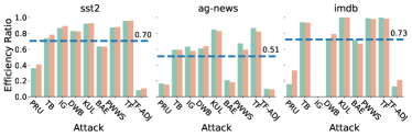
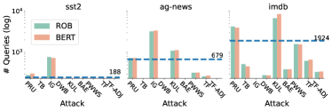
Figure 1: Efficiency of the chosen attacks. Both checklist and input reduction were tried but discarded due to low efficiency. Dashed lines report the average performance for each dataset.

Adversarial and clean sample selection. For evaluation, we rely on test sets that are made of clean samples and adversarial ones. In order to construct such sets while controlling the ratio between clean and adversarial samples, we rely on (Yoo et al., 2022, Scenario 1). From a given initial test set $\mathcal{X}_{t}$, we sample two disjoint subsets $\mathcal{X}_{1}$ and $\mathcal{X}_{2}$. We then generate attacks on $\mathcal{X}_{1}$ and take the successful one as an adversarial testing example, while $\mathcal{X}_{2}$ is taken as the clean testing sample.

4.2 Baseline detectors

We use two baseline detectors. The first one is based on a language model likelihood and the second one corresponds to the Mahalanobis detector introduced in Yoo et al. (2022). Both of them follow the analog three consecutive steps of LAROUSSE, but do not use the same similarity score.

Language model score. This method consists in computing the likelihood of an input with an external language model:

$$s_{\mathrm{LM}}(\mathbf{x})=-\sum_{i=1}^{|\mathbf{x}|}\log p_{\psi}(\omega_{i}|\omega_{i-1},\ldots,\omega_{1}),$$ (6)

where $\omega_{i}$ represents the individual token of the input sentence $\mathbf{x}$. We compute the log-probabilities with the output of a pretrained GPT2 Brown et al. (2020). Notice that this baseline is also used in Yoo et al. (2022).

Mahalanobis-based detector. We follow Yoo et al. (2022) which relies on a class-conditioned Mahalanobis distance. Following our notations, it corresponds to evaluation:

$$s_{\mathrm{M}}(\mathbf{x})=\left(f_{\psi}^{L}(\mathbf{x})-\mu_{\hat{y}}\right)^{T}\Sigma_{\hat{y}}\left(f_{\psi}^{L}(\mathbf{x})-\mu_{\hat{y}}\right),$$ (7)

where $\mu_{\hat{y}}$ is the empirical mean for the logits of class $\hat{y}$ and $\Sigma_{\hat{y}}$ is the associated empirical covariance.

Remark 3

Similarly to Remark 1, for a given textual input $\mathbf{x}$, we will either rely on the penultimate layer $L$ representation $f_{\psi}^{L}(\mathbf{x})$ or on the logits predictions $f_{\psi}^{L+1}(\mathbf{x})$ of the networks to compute $s_{M}$.

Table 2: Aggregated performance over both datasets and attacks. Each average number aggregates 270 measurements (10 seeds $\times$ 3 datasets $\times$ 9 attacks). $D_{M}$ (resp. $D_{HM}$) indicates a detector based on Mahalanobis (resp. Halspace Mass depth) (see Eq. 7), GPT to the perplexity score (see Eq. 6).

Purple color corresponds to LAROUSSE. AUROC FPR AUPR-IN AUPR-OUT Err BERT $GPT$ softmax 76.1 $\pm{9.1}$ 58.4 $\pm{19.1}$ 75.4 $\pm{8.7}$ 75.3 $\pm{10.2}$ 34.0 $\pm{9.5}$ $D_{\mathrm{M}}$ $f_{\psi}^{L}$ 88.8 $\pm{6.3}$ 49.7 $\pm{25.4}$ 90.9 $\pm{6.0}$ 84.5 $\pm{8.2}$ 28.4 $\pm{12.0}$ $f_{\psi}^{L+1}$ 90.1 $\pm{7.8}$ 32.3 $\pm{23.9}$ 88.6 $\pm{10.4}$ 88.5 $\pm{7.6}$ 19.7 $\pm{11.3}$ $D_{\mathrm{HM}}$ $f_{\psi}^{L}$ 92.0 $\pm{5.0}$ 32.1 $\pm{24.1}$ 93.3 $\pm{4.8}$ 89.4 $\pm{5.8}$ 19.5 $\pm{11.2}$ $f_{\psi}^{L+1}$ 91.9 $\pm{5.1}$ 35.8 $\pm{23.2}$ 92.4 $\pm{5.7}$ 90.0 $\pm{5.6}$ 21.4 $\pm{10.9}$ ROB. $GPT$ softmax 77.7 $\pm{9.7}$ 56.0 $\pm{20.4}$ 77.2 $\pm{9.1}$ 76.8 $\pm{10.7}$ 32.6 $\pm{9.9}$ $D_{\mathrm{M}}$ $f_{\psi}^{L}$ 89.9 $\pm{5.5}$ 44.1 $\pm{22.9}$ 91.9 $\pm{5.1}$ 86.1 $\pm{7.2}$ 25.5 $\pm{10.9}$ $f_{\psi}^{L+1}$ 90.0 $\pm{8.3}$ 31.9 $\pm{23.6}$ 88.5 $\pm{11.5}$ 88.7 $\pm{7.8}$ 19.5 $\pm{11.3}$ $D_{\mathrm{HM}}$ $f_{\psi}^{L}$ 93.4 $\pm{4.6}$ 29.0 $\pm{21.7}$ 93.9 $\pm{5.4}$ 91.3 $\pm{5.3}$ 17.9 $\pm{10.3}$ $f_{\psi}^{L+1}$ 92.8 $\pm{5.1}$ 32.1 $\pm{23.5}$ 93.3 $\pm{5.9}$ 90.9 $\pm{5.9}$ 19.4 $\pm{11.3}$

4.3 Evaluation metrics

The adversarial attack detection problem can be seen as a classification problem. In our context, two quantities are of interest, namely (i) the false alarm rate, i.e. the proportion of samples that are misclassified as adversarial sample while actually being clean; and (ii) the true detection rate, i.e., the proportion of samples that are rightfully predicted as adversarial sample. We focus on three different metrics that assess the quality of our method.

1. Area Under the Receiver Operating Characteristic curve (AUROC; Bradley (1997)). It is the area under the ROC curve which consider the true detection rate against the false alarm rate. From elementary computations, the AUROC can be linked to the probability that a clean example has higher score than an adversarial sample.

2. Area Under the Precision-Recall curve (AUPR; Davis and Goadrich (2006)). It is the area under the precision-recall curve that is more relevant to imbalanced situations. It plots the recall (true detection rate) against the precision (actual proportion of adversarial sample amongst the predicted adversarial sample).

3. False Positive Rate at 90% True Positive Rate (FPR (%)). In a practical situation, one wishes to build an efficient detector. Thus, given a detection rate $r$, this incites to fix a threshold $\delta_{r}$ such that the corresponding TPR equals $r$. Following Yoo et al. (2022), we set $r=0.90$. For FPR, lower is better.

4. Classification error (Err (%)). This refers to the lowest classification error obtained by choosing the best-fixed threshold.

5 Experimental results

5.1 Overall Results

We report in Tab. 2 the aggregated performance over the different datasets, the various seeds, and the different attacks.
$D_{\mathrm{HM}}$ achieves the best overall results. It is worth noting that detection methods better discriminate adversarial attacks on ROB. than BERT. It also consistently improves the performance when using a halfspace mass score $D_{\mathrm{HM}}$ instead of Mahanalobis $D_{\mathrm{M}}$, which experimentally validates our choice. This conclusion holds on both ROB. and BERT, corresponding to over $540$ experimental configurations. Similar to previous work Yoo et al. (2022), the detector built on GPT2 under-performs $D_{\mathrm{M}}$. For all methods, we observe that LAROUSSE achieves the best results both in terms of threshold-free (e.g. AUROC, AUPR-IN and AUPR-OUT) threshold-based metrics (e.g. FPR) which validates our detector.

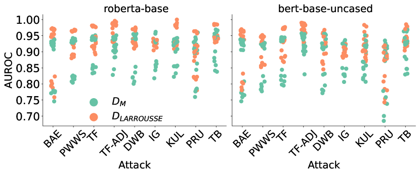
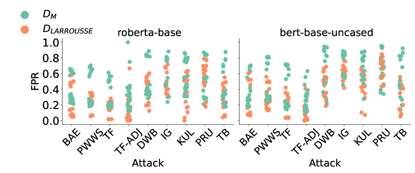
Figure 2: Performance per attack in for each pretrained encoder in terms of AUROC (left) and FPR (right) of $D_{\mathrm{M}}$ and $D_{\mathrm{HM}}$ on STAKEOUT.

Importance of feature selection for adversarial detectors. Both $D_{\mathrm{HM}}$ and $D_{\mathrm{M}}$ are highly sensitive to the layer’s choice. For $D_{\mathrm{M}}$, using the logits is better than the penultimate layer, while for $D_{\mathrm{HM}}$, the converse works better. Although the AUROC presents a slight variation when using $f_{\psi}^{L+1}$ instead of $f_{\psi}^{L}$, it induces a variation of over 10 FPR points.

Overall, it is worth noting that LAROUSSE, although being state-of-the-art on tested configurations, achieves an FPR which remains moderate. The best-averaged error of $17.9\%$ is far from the error achieved on the main task (less than 10% on all datasets).

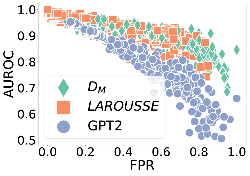
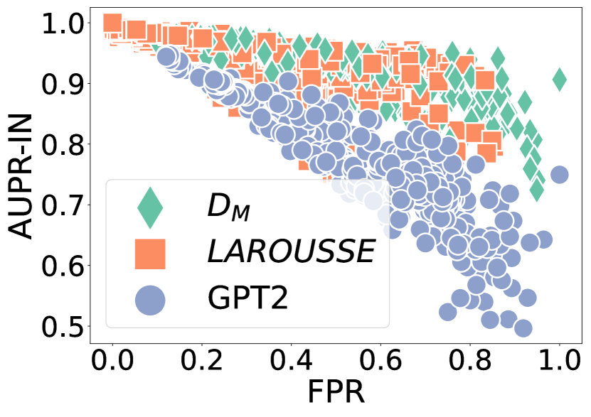
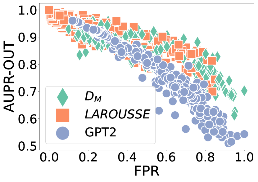
Figure 3: Empirical study of the metric relationship for the three considered detection methods.

5.2 Identifying key detection factors

To better understand the performance of our methods w.r.t different attacks and various datasets, we report in Fig. 4 the performance in terms of AUROC and FPR per attack.
Detectors and models are not robust to dataset change. The detection task is more challenging for SST-2 than for ag-news and IMDB, with a significant drop in performance (e.g. over 15 absolute points for BAE). On SST-2, $D_{\mathrm{HM}}$ achieves a significant gain over $D_{\mathrm{M}}$ both for the AUROC and FPR.
Detectors do not detect uniformly well the various attacks. This phenomenon is pronounced on SST2 while being present for both ag-news and IMDB. For example on SST2, FPR varies from less than 10 (a strong detection performance) for TF-ADJ to over 70 (a poor performance) for PRU.
Hard to detect attack for ROB. are not necessarily hard to detect for BERT. This phenomenon is illustrated by Fig. 2. For example, KUL is hard to detect for BERT while being easier on ROB as LAROUSSE achieves over 96 AUROC points. If safety is a primary concern, it is thus crucial to carefully select the pre-trained encoder.
The choice of clean samples largely affects the detection performance measure. Fig. 4 and Fig. 2 display several tries with different seeds. As mentioned in Sec. 4, different seeds correspond to various choices of clean samples. On all datasets, we observe that when measuring the algorithm performance, different negative samples will lead to different results (e.g. FPR on IMDB varies of over 30 points on KUL and PRU across different seeds).

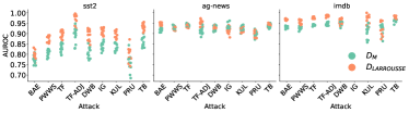
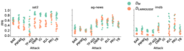
Figure 4: Performance in terms of AUROC (up) and FPR (down) of $D_{\mathrm{M}}$ and $D_{\mathrm{HM}}$ on STAKEOUT. Fig. 7 in the Supplementary Material reports the results of GPT2.

5.3 All the metrics matter

Setting. In this experiment, we study the relationship between the different metrics. From Tab. 2, we see that threshold free metrics (i.e., AUROC, AUPR-IN) exhibit lower variance than threshold based metrics such as FPR. The FPR measures the percentage of natural samples detected as adversarial when $90\%$ of the attacked samples are detected. Therefore, the lower, the better.
Takeaways. From Fig. 3, we see that for a large AUROC, AUPR-IN and AUPR-OUT do not necessarily corresponds a low FPR. This suggests that the detectors also detect natural samples as adversarial when it detect at least 90$\%$ of adversarial examples. Additionally, a small variation of AUROC, AUPR-IN and AUPR-OUT can lead to a high change in FPR. It is therefore crucial to compare the detectors using all metrics.

5.4 Expected performances of LAROUSSE

Setting. Fig. 5 reports the error probability per attack for LAROUSSE and the considered baselines.

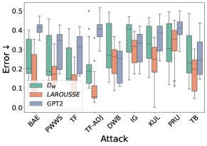
Figure 5: Detection error on STAKEOUT.

Efficient attacks are easier to detect. We observe that on the three most efficient attacks, according to Fig. 1 (i.e., TF, PWWS and KUL), LAROUSSE is significantly more effective than $D_{\mathrm{M}}$ and GPT2.
Different detection methods capturing various phenomena are better suited for detecting types of attack. Although LAROUSSE achieves the best results overall, GPT2, which relies on perplexity solely, achieves competitive results with LAROUSSE and outperforms $D_{\mathrm{M}}$ on several attacks (i.e., DWB and IG). This suggests that stronger detectors could be achieve by combining different types of scoring functions.

5.5 Semantic vs syntactic attacks

In this section, we analyze the results of the LAROUSSE on semantic (i.e., working on token) versus syntactic (i.e, working on character) attacks. Raw and processed results are reported in Sec. 10.5.

Takeaways. From 9, we observe that semantic attacks are harder to detect for both our method and $D_{H}$.

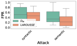
Figure 6: FPR for semantic vs syntactic analysis further results can be found in 9

6 Concluding Remarks

We have proposed STAKEOUT, a large adversarial attack detection benchmark, and LAROUSSE. LAROUSSE leverages a new anomaly score built on the halfspace-mass depth and offers a better alternative than the widely known Mahalanobis distance.

7 Ethical impact of our work

Our work focuses on responsive NLP and aims at contributing to the protection of NLP systems. Our new benchmark STAKEOUT allows for a robust evaluation of new adversarial detection methods. And LAROUSSE outperforms previous methods and thus provides a better defense against attackers. Overall, we believe this paper offers promising research direction toward safe and robust NLP systems and will benefit the community.

[sections] [sections]l1

8 Approximation algorithms

In this section, we present the algorithms, originally proposed in Chen et al. [2015] and adapted to our problem, to approximate $D_{HM}$ that is used in LAROUSSE (see Algorithm 1 for the training and Algorithm 2 for the testing).

8.1 Computational aspects

The first step is to draw uniformly at random a set of closed halfspaces of $\mathbb{R}^{d}$. Drawing a halfspace is equivalent to drawing a hyperplane, which is accomplished by sampling a direction $u$ from the unit hypersphere $\mathbb{S}^{d-1}$ as well as a threshold ruled by a hyperparameter $\lambda$ that both uniquely define a hyperplane/halfspace. To avoid halfspaces carrying no information, thresholds are chosen such that at least one training sample belongs to each of the constructed halfspaces requiring to project the training set on $u$. This procedure is repeated $K\geq 1$ times, where $K$ is chosen by the user as is $\lambda$. The computation can be accelerated by performing this procedure on a subsample of the training set. The training part, which is outlined in Algorithm 1 in Appendix 8, allows to obtain $K$ closed halfspaces as well as their $K$ complementary spaces leading to $2K$ halfspaces. The test part lie in evaluating the depth score of any new observation $\mathbf{x}\in\mathbb{R}^{d}$ by using the pre-defined halfspaces. Indeed, $\mathbf{x}$ belongs to $K$ among the $2K$ constructed halfspaces during the training step. The goal is then to compute the probability mass, i.e., the proportion of training samples in the $K$ halfspaces to which $\mathbf{x}$ belongs and then, compute the mean values of these proportions. This testing step is outlined in the Algorithm 2 in Appendix 8.

Algorithm 1 Training algorithm for the approximation of $D_{\mathrm{HM}}$.

INPUT: sample $\mathcal{D}_{y}=\{f_{\psi}^{L}(\mathbf{x}_{i})\;:\;y_{i}=y\}$.

INIT: Number of halfspaces $K$; sub-sample size $n_{s}$; hyperparameter $\lambda$.

1:for  $k=1,\ldots,K$ do

2:     Draw $\mathcal{D}_{y,n_{s}}$, a sub-sample of $\mathcal{D}_{y}$ with size $n_{s}$ without replacement.

3:     Draw randomly and uniformly a direction $u_{k}$ in $\mathbb{S}^{d-1}$.

4:     Compute $\langle u_{k},f_{\psi}^{L}(\mathbf{x}_{i})\rangle$ for every $f_{\psi}^{L}(\mathbf{x}_{i})\in\mathcal{D}_{y,n_{s}}$ such that $p_{k,i}\triangleq\langle u_{k},f_{\psi}^{L}(\mathbf{x}_{i})\rangle$.

5:     Set $\mathrm{mid}_{k}=\big{(}\underset{i}{\max}~{}p_{k,i}+\underset{i}{\min}~{}p_{k,i}\big{)}/2$ and $\mathrm{range}_{k}=\underset{i}{\max}~{}p_{k,i}-\underset{i}{\min}~{}p_{k,i}$.

6:     Randomly and uniformly select $\kappa_{k}$ in $\big{[}\mathrm{mid}_{k}-\frac{\lambda}{2}\mathrm{range}_{k},\;\mathrm{mid}_{k}+\frac{\lambda}{2}\mathrm{range}_{k}\big{]}$.

7:     Set $m_{k}^{\mathrm{left}}=\dfrac{|\{\mathbf{z}\in\mathcal{D}_{y,n_{s}}:\;p_{k,i}<\kappa_{k}\}|}{n_{s}}$ and $m_{k}^{\mathrm{right}}=\dfrac{|\{\mathbf{z}\in\mathcal{D}_{y,n_{s}}:\;p_{k,i}\geq\kappa_{k}\}|}{n_{s}}$.

8:end for

OUTPUT: $\{u_{k},\kappa_{k},m_{k}^{\mathrm{left}},m_{k}^{\mathrm{right}}\}_{k=1}^{K}$.

Algorithm 2 Testing algorithm for the approximation of $D_{\mathrm{HM}}$.

INPUT: test observation $f_{\psi}^{L}(\mathbf{x})$; $\{u_{k},\kappa_{k},m_{k}^{\mathrm{left}},m_{k}^{\mathrm{right}}\}_{k=1}^{K}$.

INIT: HM=0.

1:for  $k=1,\ldots,K$ do

2:     Project $f_{\psi}^{L}(\mathbf{x})$ onto $u_{k}$ and such that $p_{k}^{\ell}=\langle f_{\psi}^{L}(\mathbf{x}),u_{k}\rangle$.

3:     HM = HM + $m_{k}^{\mathrm{left}}~{}\mathbb{I}(p_{k}^{\ell}<\kappa_{k})$ + $m_{k}^{\mathrm{right}}~{}\mathbb{I}(p_{k}^{\ell}\geq\kappa_{k})$.

4:end for

OUTPUT: $D_{\mathrm{HM}}(f_{\psi}^{L}(\mathbf{x}),\mathcal{D}_{y})=\text{HM}/K$.

9 Additional Details on STAKEOUT Construction

For completeness, we regroup in Tab. 3 additional details on the attacks used in STAKEOUT.

In this paper we focused our evaluation on existing attacks. In the future, a possible extension of STAKEOUT would be to use the methodology of Dynabench Kiela et al. [2021] and rely on human feedback to attack the model.

Table 3: Considered attacks for STAKEOUT construction.

Full Name	Acronym	Idea	Type of Constraint
pruthi Pruthi et al. [2019]	PRU	Simulation of common typos using greedy search for untargeted classification	Minimum word length, maximum number of words perturbed
textbugger Li et al. [2018]	TB	Character-based attack (i.e swap, deletion, subtitution)	Cosine with USE Cer et al. [2018]
iga Wang et al. [2019]	IG	Genetic algorithm to perform word substitution	Percentage of perturbed words and word embedding distance on Word2Vect Mikolov et al. [2013]
deepwordbug Gao et al. [2018]	DWB	Character-based attack (i.e swap, deletion, subtitution)	Levenshtein distance Levenshtein [1965]
kuleshov Kuleshov et al. [2018]	KUL	Attack using embedding swap	Cosine and language model similarity
clareLi et al. [2021]	CLA	Attack using token insertion, merge and swap	Embedding similarity
bae Garg and Ramakrishnan [2020]	BAE	Attack using BERT MLM combined with a greedy search	Number of perturbed words and cosine with USE Cer et al. [2018]
pwws Ren et al. [2019]	PWWS	Word swap based on WordNet synonyms
textfooler Jin et al. [2020]	TF	Attack using embedding swap	Embedding similarity and POS match with word and embedding swap
TF-adjustedMorris et al. [2020a]	TF-ADF	Attack using embedding swap	USE and word embedding similarity
input-reduction Feng et al. [2018]	IR	Greedy attack using word importance ranking via greedy search
checklist Ribeiro et al. [2020]	CHK	Using contraction/extension and changing numbers, locations, names

10 Additional Results

This section gathers additional experimental results to allow the curious reader to draw fine conclusions. Formally, we conduct:

• a detailed analysis of the detectors’ performances per attack (see Sec. 10.1).

• a detailed analysis of the detectors’ performances per dataset across all the considered metrics (see Sec. 10.2).

• the extended figures of Sec. 5.2 (see Sec. 10.3).

• an analysis per dataset/per attack of the different detector performances on STAKEOUT in Sec. 10.4.

• an comparative study of the detector’s performance between semantic and syntactic attacks.

• an in-depth reflection on the possibility of building multi-layer detectors (see Sec. 10.6).

10.1 Fine grained analysis per attack

In Tab. 4, we report the average performances on STAKEOUT for each detector on each model under each attack’s threat. First, it is interesting to note that LAROUSSE strongly outperforms other methods on most of the configurations. Then, corroborating previous observations, we find that changing attacks, encoders, and metrics largely influence the detection performances.
Takeaways. These findings validate our extended STAKEOUT, as in real-life scenario, practitioners need to ensure that the detection methods works well on a large number of attacks for different types of models.

Table 4: Average performances on STAKEOUT per model and per attack

			AUROC	FPR	AUPR-IN	AUPR-OUT	Err
BERT	$D_{M}$	BAE	87.5 $\pm{7.6}$	39.3 $\pm{20.3}$	88.5 $\pm{8.8}$	84.1 $\pm{8.0}$	24.6 $\pm{10.1}$
		DWB	88.6 $\pm{6.8}$	60.0 $\pm{24.3}$	90.8 $\pm{5.7}$	84.7 $\pm{9.2}$	32.4 $\pm{12.1}$
		IG	87.8 $\pm{5.0}$	72.0 $\pm{15.2}$	90.7 $\pm{4.1}$	82.3 $\pm{7.2}$	38.2 $\pm{7.7}$
		KUL	88.2 $\pm{4.7}$	67.4 $\pm{17.6}$	90.9 $\pm{4.0}$	83.1 $\pm{6.9}$	35.8 $\pm{8.9}$
		PRU	84.6 $\pm{8.6}$	67.0 $\pm{21.8}$	86.9 $\pm{7.8}$	80.5 $\pm{10.2}$	35.7 $\pm{10.7}$
		PWWS	88.0 $\pm{6.2}$	44.3 $\pm{23.7}$	90.7 $\pm{5.1}$	82.5 $\pm{8.9}$	27.1 $\pm{11.9}$
		TB	91.5 $\pm{4.9}$	51.3 $\pm{25.0}$	93.6 $\pm{3.8}$	87.7 $\pm{7.3}$	28.1 $\pm{12.5}$
		TF	89.8 $\pm{6.1}$	34.9 $\pm{23.0}$	91.6 $\pm{5.9}$	85.6 $\pm{8.0}$	22.4 $\pm{11.5}$
		TF-ADJ	92.3 $\pm{2.9}$	27.3 $\pm{14.8}$	94.4 $\pm{2.0}$	88.8 $\pm{5.1}$	18.3 $\pm{7.2}$
	$GPT$	BAE	68.4 $\pm{3.8}$	73.0 $\pm{5.4}$	67.8 $\pm{3.8}$	66.5 $\pm{4.1}$	41.4 $\pm{2.7}$
		DWB	85.5 $\pm{7.0}$	38.8 $\pm{17.4}$	84.4 $\pm{7.3}$	86.0 $\pm{6.9}$	24.3 $\pm{8.6}$
		IG	80.8 $\pm{4.8}$	53.5 $\pm{16.0}$	80.1 $\pm{4.7}$	78.8 $\pm{6.7}$	31.5 $\pm{8.0}$
		KUL	74.2 $\pm{7.3}$	65.1 $\pm{14.2}$	74.2 $\pm{6.8}$	73.0 $\pm{8.3}$	36.9 $\pm{6.5}$
		PRU	67.7 $\pm{7.4}$	74.2 $\pm{9.1}$	68.2 $\pm{7.5}$	66.0 $\pm{6.8}$	41.9 $\pm{4.5}$
		PWWS	77.9 $\pm{8.5}$	53.7 $\pm{18.6}$	76.3 $\pm{8.8}$	78.0 $\pm{9.4}$	31.8 $\pm{9.3}$
		TB.	82.8 $\pm{6.2}$	46.7 $\pm{19.3}$	81.5 $\pm{5.8}$	82.5 $\pm{8.2}$	28.2 $\pm{9.6}$
		TF	80.2 $\pm{7.9}$	48.6 $\pm{18.5}$	78.3 $\pm{7.9}$	80.6 $\pm{9.3}$	29.2 $\pm{9.2}$
		TF-ADJ	69.2 $\pm{4.7}$	70.3 $\pm{9.1}$	69.8 $\pm{4.5}$	67.9 $\pm{6.1}$	39.5 $\pm{4.9}$
	$D_{HM}$	BAE	91.3 $\pm{7.2}$	22.9 $\pm{20.6}$	91.8 $\pm{8.1}$	89.4 $\pm{7.0}$	16.4 $\pm{10.3}$
		DWB	91.6 $\pm{3.7}$	48.8 $\pm{15.0}$	93.0 $\pm{3.6}$	88.8 $\pm{3.8}$	26.8 $\pm{7.5}$
		IG	90.1 $\pm{1.3}$	60.9 $\pm{9.1}$	92.2 $\pm{1.7}$	86.6 $\pm{1.9}$	32.7 $\pm{4.3}$
		KUL	91.9 $\pm{3.4}$	47.0 $\pm{17.5}$	93.0 $\pm{3.2}$	90.2 $\pm{4.4}$	25.6 $\pm{9.0}$
		PRU	85.8 $\pm{5.9}$	68.9 $\pm{12.9}$	88.4 $\pm{5.4}$	81.8 $\pm{6.2}$	36.7 $\pm{6.4}$
		PWWS	91.3 $\pm{3.7}$	28.6 $\pm{15.4}$	93.0 $\pm{3.5}$	87.9 $\pm{4.0}$	19.3 $\pm{7.7}$
		TB	94.6 $\pm{2.4}$	32.7 $\pm{16.4}$	95.7 $\pm{2.2}$	92.3 $\pm{2.9}$	18.8 $\pm{8.2}$
		TF	93.3 $\pm{3.9}$	18.3 $\pm{13.2}$	94.1 $\pm{4.3}$	91.5 $\pm{3.9}$	14.1 $\pm{6.6}$
		TF-ADJ	96.9 $\pm{2.0}$	7.9 $\pm{10.7}$	97.8 $\pm{1.2}$	95.3 $\pm{4.3}$	8.4 $\pm{5.3}$
ROB	$D_{M}$	BAE	87.5 $\pm{7.4}$	39.4 $\pm{16.8}$	88.7 $\pm{8.2}$	84.4 $\pm{7.7}$	24.6 $\pm{8.4}$
		DWB	90.4 $\pm{6.0}$	52.4 $\pm{23.2}$	92.4 $\pm{4.9}$	86.6 $\pm{8.4}$	28.6 $\pm{11.6}$
		IG	89.6 $\pm{5.0}$	60.8 $\pm{22.0}$	92.0 $\pm{3.9}$	85.2 $\pm{7.5}$	32.7 $\pm{11.0}$
		KUL	90.1 $\pm{4.2}$	57.0 $\pm{20.1}$	92.3 $\pm{3.6}$	85.5 $\pm{5.8}$	30.7 $\pm{10.1}$
		PRU	87.5 $\pm{6.8}$	55.3 $\pm{23.6}$	89.6 $\pm{5.6}$	84.2 $\pm{9.0}$	29.8 $\pm{11.9}$
		PWWS	89.5 $\pm{5.7}$	36.0 $\pm{20.7}$	91.6 $\pm{5.1}$	85.0 $\pm{7.2}$	22.9 $\pm{10.3}$
		TB	92.5 $\pm{4.6}$	44.9 $\pm{22.5}$	94.3 $\pm{3.5}$	89.1 $\pm{6.9}$	24.9 $\pm{11.2}$
		TF	91.0 $\pm{4.6}$	29.5 $\pm{17.3}$	92.7 $\pm{4.3}$	87.3 $\pm{6.1}$	19.7 $\pm{8.6}$
		TF-ADJ	91.3 $\pm{3.3}$	33.2 $\pm{21.2}$	93.6 $\pm{2.3}$	87.2 $\pm{5.6}$	20.5 $\pm{9.6}$
	$GPT$	BAE	69.3 $\pm{4.9}$	71.6 $\pm{6.9}$	68.0 $\pm{4.8}$	67.4 $\pm{5.4}$	40.7 $\pm{3.4}$
		DWB	88.4 $\pm{5.2}$	31.5 $\pm{13.7}$	87.4 $\pm{5.6}$	88.8 $\pm{5.3}$	20.6 $\pm{6.8}$
		IG	82.5 $\pm{5.5}$	51.0 $\pm{16.1}$	82.3 $\pm{5.2}$	80.6 $\pm{7.2}$	30.2 $\pm{8.1}$
		KUL	73.6 $\pm{8.3}$	66.0 $\pm{16.1}$	73.7 $\pm{7.0}$	72.6 $\pm{9.5}$	37.1 $\pm{7.2}$
		PRU.	68.7 $\pm{9.3}$	71.3 $\pm{10.6}$	69.8 $\pm{8.8}$	67.7 $\pm{7.6}$	40.0 $\pm{4.8}$
		PWWS.	80.0 $\pm{7.3}$	50.8 $\pm{17.6}$	78.9 $\pm{7.1}$	79.4 $\pm{8.8}$	30.4 $\pm{8.8}$
		TB	85.8 $\pm{5.0}$	39.8 $\pm{17.3}$	84.9 $\pm{4.4}$	85.4 $\pm{7.4}$	24.8 $\pm{8.6}$
		TF	81.5 $\pm{7.5}$	47.6 $\pm{18.2}$	80.0 $\pm{7.6}$	81.3 $\pm{8.9}$	28.7 $\pm{9.1}$
		TF-ADJ	71.0 $\pm{5.5}$	72.6 $\pm{10.3}$	71.9 $\pm{5.3}$	68.9 $\pm{7.4}$	40.5 $\pm{4.5}$
	$D_{HM}$	BAE	90.7 $\pm{7.9}$	22.0 $\pm{19.6}$	90.3 $\pm{10.1}$	89.4 $\pm{6.8}$	15.9 $\pm{9.8}$
		DWB	93.9 $\pm{2.4}$	37.4 $\pm{15.7}$	94.5 $\pm{2.8}$	91.8 $\pm{3.7}$	21.1 $\pm{7.9}$
		IG	92.5 $\pm{1.0}$	47.8 $\pm{15.4}$	93.5 $\pm{1.7}$	89.3 $\pm{2.8}$	26.1 $\pm{7.5}$
		KUL	94.2 $\pm{3.3}$	36.5 $\pm{20.3}$	94.6 $\pm{3.6}$	92.7 $\pm{4.4}$	20.3 $\pm{10.6}$
		PRU	89.0 $\pm{5.7}$	55.1 $\pm{21.1}$	89.8 $\pm{6.6}$	86.2 $\pm{7.1}$	29.7 $\pm{10.8}$
		PWWS	92.8 $\pm{3.3}$	20.5 $\pm{12.0}$	93.4 $\pm{4.4}$	90.1 $\pm{3.7}$	15.2 $\pm{6.0}$
		TB	95.7 $\pm{2.2}$	26.4 $\pm{17.8}$	96.4 $\pm{1.9}$	93.8 $\pm{3.8}$	15.6 $\pm{8.9}$
		TF	94.3 $\pm{3.1}$	14.2 $\pm{10.3}$	94.7 $\pm{3.9}$	92.5 $\pm{3.7}$	12.0 $\pm{5.2}$
		TF-ADJ	96.8 $\pm{2.8}$	10.5 $\pm{16.5}$	97.7 $\pm{1.8}$	94.9 $\pm{4.9}$	9.2 $\pm{8.3}$

10.2 Fine grained analysis per dataset

We report in Tab. 5, the performances on STAKEOUT averaged over the datasets for different detector configurations. We observe that LAROUSSE achieves the best results on 2 out of the 3 datasets. Overall, it is interesting to note that LAROUSSE’s performances are more consistent compared to Mahanalobis when changing the feature representation (i.e., using $f_{\theta}^{L}$ instead of $f_{\theta}^{L+1}$).
Takeaways. This validates that the half-space mass is better for detecting textual adversarial attacks than the widely used Mahanalobis score.

Table 5: Average performance on STAKEOUT per training dataset.

			AUROC	FPR	AUPR-IN	AUPR-OUT	Err
ag-news	$D_{M}$	$f_{\theta}^{L}$	92.5 $\pm{1.6}$	37.2 $\pm{14.3}$	94.1 $\pm{1.3}$	89.9 $\pm{2.3}$	22.2 $\pm{6.2}$
		$f_{\theta}^{L+1}$	94.8 $\pm{2.1}$	23.9 $\pm{17.3}$	95.6 $\pm{2.3}$	93.0 $\pm{2.7}$	15.5 $\pm{7.7}$
	$GPT2$	$f_{\theta}^{L}$	84.1 $\pm{8.2}$	41.5 $\pm{20.3}$	83.2 $\pm{7.9}$	84.2 $\pm{9.3}$	25.6 $\pm{10.1}$
	LAROUSSE		92.8 $\pm{1.9}$	39.8 $\pm{21.4}$	94.8 $\pm{1.5}$	88.7 $\pm{2.8}$	23.4 $\pm{9.6}$
	$D_{HM}$	$f_{\theta}^{L+1}$	91.9 $\pm{2.1}$	46.1 $\pm{18.8}$	93.9 $\pm{1.7}$	88.6 $\pm{2.9}$	26.5 $\pm{8.3}$
imdb	$D_{M}$	$f_{\theta}^{L}$	93.6 $\pm{2.1}$	30.5 $\pm{17.5}$	95.3 $\pm{1.6}$	90.2 $\pm{3.5}$	18.9 $\pm{7.9}$
		$f_{\theta}^{L+1}$	94.2 $\pm{3.8}$	18.6 $\pm{18.0}$	93.9 $\pm{5.4}$	92.6 $\pm{4.0}$	12.9 $\pm{8.2}$
	$GPT2$	$f_{\theta}^{L}$	71.7 $\pm{8.7}$	63.8 $\pm{15.4}$	70.5 $\pm{7.7}$	72.3 $\pm{9.8}$	36.4 $\pm{7.4}$
	LAROUSSE		96.6 $\pm{2.3}$	14.5 $\pm{17.3}$	97.3 $\pm{1.8}$	95.2 $\pm{3.3}$	10.8 $\pm{7.9}$
	$D_{HM}$	$f_{\theta}^{L+1}$	96.7 $\pm{2.7}$	12.8 $\pm{15.9}$	96.7 $\pm{3.9}$	95.6 $\pm{3.6}$	9.9 $\pm{7.3}$
sst2	$D_{M}$	$f_{\theta}^{L}$	82.4 $\pm{4.7}$	71.3 $\pm{17.5}$	85.2 $\pm{5.1}$	76.3 $\pm{5.6}$	39.0 $\pm{8.1}$
		$f_{\theta}^{L+1}$	81.6 $\pm{7.7}$	52.4 $\pm{20.0}$	76.7 $\pm{10.0}$	80.6 $\pm{7.2}$	29.6 $\pm{9.7}$
	$GPT2$	$f_{\theta}^{L}$	74.3 $\pm{6.3}$	67.0 $\pm{11.4}$	74.7 $\pm{6.0}$	71.3 $\pm{6.8}$	38.2 $\pm{5.5}$
	LAROUSSE		88.7 $\pm{5.7}$	42.8 $\pm{19.3}$	88.8 $\pm{6.0}$	87.3 $\pm{6.4}$	24.6 $\pm{9.5}$
	$D_{HM}$	$f_{\theta}^{L+1}$	88.6 $\pm{5.9}$	42.4 $\pm{19.4}$	88.0 $\pm{6.7}$	87.3 $\pm{6.2}$	24.5 $\pm{9.4}$

10.3 Extended figures for Sec. 5.2

We report in Fig. 7 the extended figures for Sec. 5.2. The baseline detector built on GPT2 is weaker than $D_{M}$ and LAROUSSE, and consistantly achieves lower results in term of AUROC, AUPR-IN, AUPR-OUT and FPR.

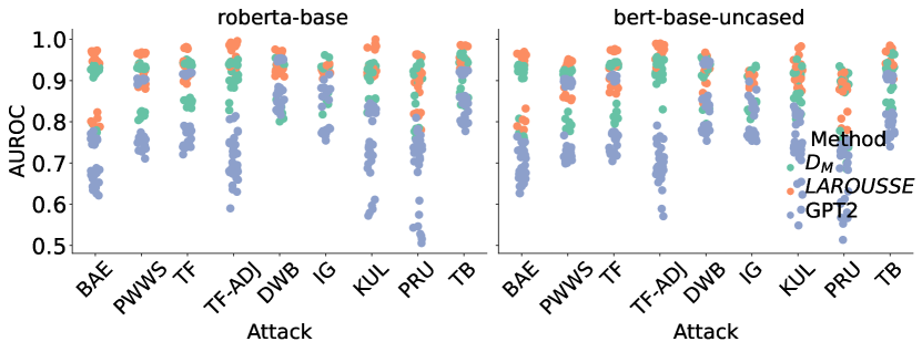
AUROC

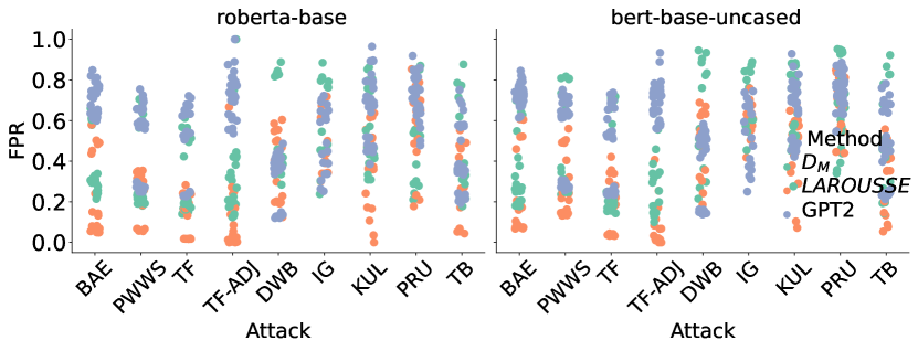
FPR

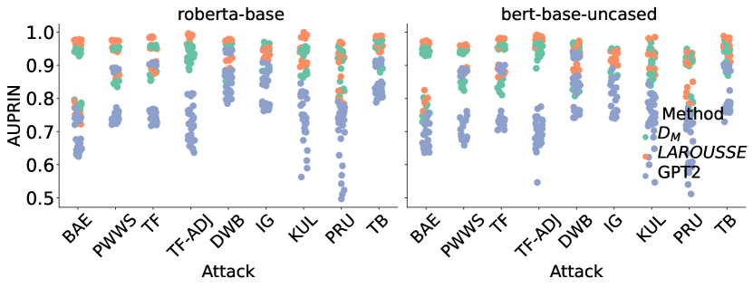
AUPR-IN

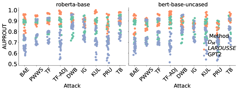
AUPR-OUT

Figure 7: Extended figures for Sec. 5.2. In these figures, we report the GPT2 baseline and the performance of all the detectors in terms of AUROC, AUPR-IN, AUPR-OUT and FPR.

10.4 Analysis per dataset/per attack

We report in Fig. 8 the different detectors’ performances in terms of AUROC, AUPR-IN, AUPR-OUT and FPR for the different datasets. Similar to what has been previously observed, we see a large variation in the different detectors’ performance when changing both the dataset and the type of attack.

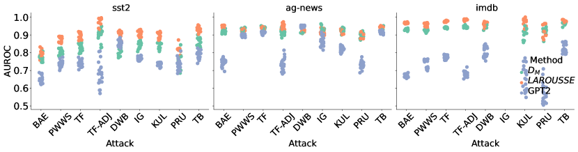
AUROC

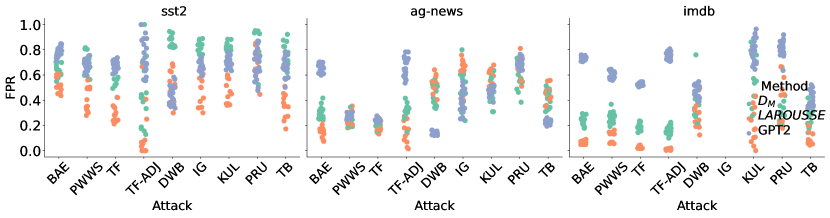
FPR

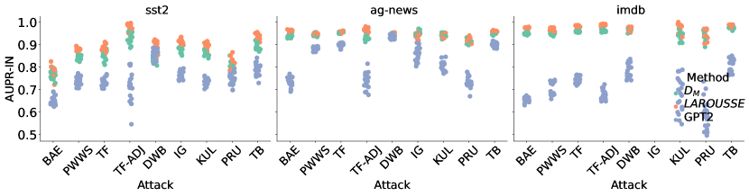
AUPR-IN

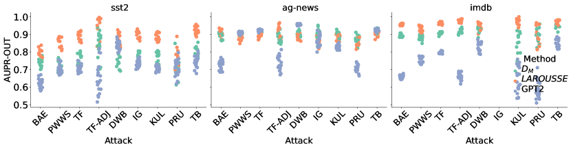
AUPR-OUT

Figure 8: Detectors performance per datasets in terms of AUROC, AUPR-IN, AUPR-OUT and FPR.

10.5 Comparing detection performance between semantic versus syntactic attacks

In this section, we analyse results of the LAROUSSE on semantic (i.e., working on token) versus syntactic (i.e, working on character) attacks. Raw and processed results are reported in LABEL:fig:semantic_analysis.

Takeaways. From 9, we observe that semantic attacks are harder to detect for both our method and $D_{H}$.

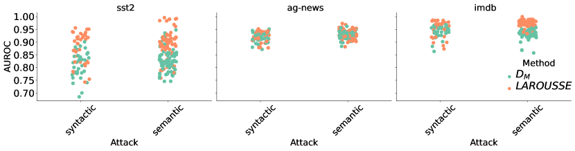
AUROC

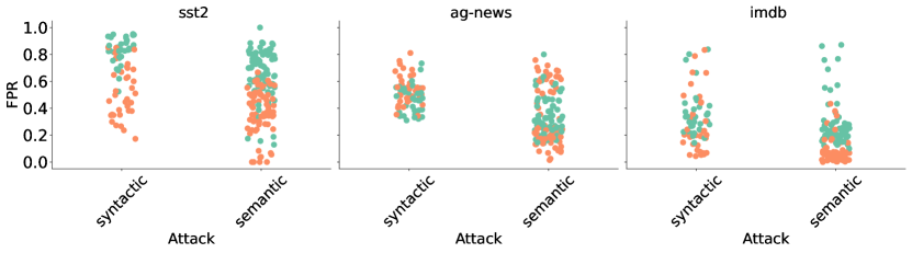
FPR

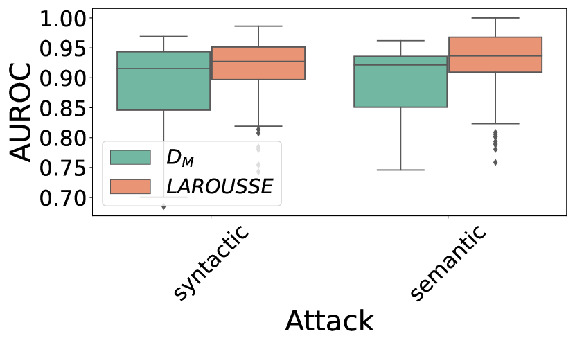
AUROC

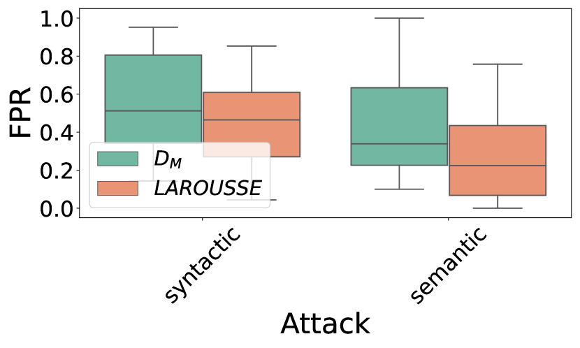
FPR

Figure 9: In these figures we report the results of the semantic versus syntactic analysis in terms of AUROC and FPR.

10.6 Towards multi-layer detectors

A promising research direction to improve the detection methods is to develop an unsupervised strategy to combine multiple-layer representations of the pre-trained encoders Gomes et al. [2022], Sastry and Oore [2020]. To the best of our knowledge, this has never been shown to be useful for text data.

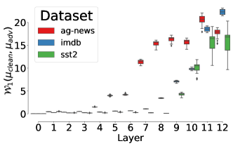
Figure 10: $\mathcal{W}_{1}\left(\mu_{clean},\mu_{adv}\right)$.

Setting. In this experiment, we aim to quantify the power of each layer to discriminate between clean and adversarial samples. To measure this ability, we rely on Wasserstein distance ($\mathcal{W}_{1}$; see Peyré and Cuturi [2019]). Given two empirical distributions, $\mathcal{W}_{1}$ finds the best possible transfer between them while minimizing the transportation cost defined by the Euclidean distance. Fig. 10 reports the transportation cost ($\mathcal{W}_{1}$) between the empirical distributions of clean samples ($\mu_{clean}$) and adversarial samples ($\mu_{adv}$) obtained at each layer.
Analysis. The last layers of the encoder have a better ability to discriminate the adversarial samples from the clean one than the first layers. Similarly to what can be observed in Fig. 3, we observe that IMDB is the easiest dataset as the last encoder layer can better distinguish the adversarial samples and the clean one. Interestingly, we observe that the best layer depends on the dataset, which is consistent with the observation in NLG evaluation Zhang* et al. [2020], where the optimal layer is found using a validation set. Overall, the information present at the last encoder layers suggests that designing multi-layer detectors is a promising research direction.

10.7 Attacking our detectors

Adversarial attack detection methods have been extensively studied in the computer vision community Feinman et al. [2017], Ma et al. [2018], Kherchouche et al. [2020], Aldahdooh et al. [2022b, a] and recently a line of work on adaptive attacks Carlini and Wagner [2017], Athalye et al. [2018], Tramer et al. [2020] have emerged. LAROUSSE is not differentiable adding an extra layer of security: it prevents the malicious adversaries to leverage gradient computations, contrary to studied baselines (e.g Mahalanobis, GPT). Attacking LAROUSSE is thus a quite challenging research question that falls outside of the scope of the paper and is left as future work.

11 Future work

In the future, we would like to extend our adversarial detection setting to natural language generation tasks on seq2seq models Pichler et al. [2022], Colombo et al. [2019, 2021d, 2021b] and classification tasks Chapuis et al. [2020], Colombo et al. [2022d, b], Himmi et al. [2023] as well as NLG evaluation Colombo et al. [2021e, 2022c, c, a, b] and Safe AI Colombo et al. [2022a], Picot et al. [2022a, b], Darrin et al. [2022, 2023].

12 Computation time comparison between HM and Mahalanobis depths

In this part, we compare the computation time between the HM and the Mahalanobis depths. Precisely, we want to compare the time of computing these data depths of an element $x\in\mathbb{R}^{d}$ w.r.t. a dataset. This experiment is conducted as follows: several datasets (varying dimension $\{800,1000,1200,1500,2000,2500,5000\}$ and sample size $\{100,2500,5000,7500,10000\}$) are sampled from centered Gaussian distributions $\mathcal{N}(0,\Sigma)$ where $\Sigma$ follows a Wishart distribution. Therefore, we compute the depth of $\mathbf{0}$ w.r.t. each of these datasets. This procedure is repeated 10 times. We report their mean computation time as well as 10-90% quantiles in Figure 11 highlighting the computational benefits of using the HM depth over the Mahalanobis distance. The dimension is 5000 on the left picture while the sample size is fixed to 100 on the right picture.

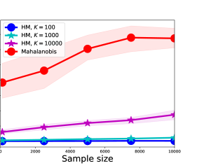
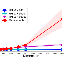
Figure 11: Computation time of HM ($K\in\{100,1000,10000\}$) and Mahalanobis depths for various sample sizes (left) and dimensions (right).

References

- Aldahdooh et al. [2022a] Ahmed Aldahdooh, Wassim Hamidouche, and Olivier Déforges. Revisiting model’s uncertainty and confidences for adversarial example detection. Applied Intelligence, pages 1–23, 2022a.
- Aldahdooh et al. [2022b] Ahmed Aldahdooh, Wassim Hamidouche, Sid Ahmed Fezza, and Olivier Déforges. Adversarial example detection for dnn models: A review and experimental comparison. Artificial Intelligence Review, pages 1–60, 2022b.
- Alves et al. [2018] Erin Alves, Devesh Bhatt, Brendan Hall, Kevin Driscoll, Anitha Murugesan, and John Rushby. Considerations in assuring safety of increasingly autonomous systems. NASA, 2018.
- Alzantot et al. [2018] Moustafa Alzantot, Yash Sharma, Ahmed Elgohary, Bo-Jhang Ho, Mani Srivastava, and Kai-Wei Chang. Generating natural language adversarial examples. In Proceedings of the 2018 Conference on Empirical Methods in Natural Language Processing, pages 2890–2896, Brussels, Belgium, October-November 2018. Association for Computational Linguistics. doi: 10.18653/v1/D18-1316. URL https://aclanthology.org/D18-1316.
- Athalye et al. [2018] Anish Athalye, Nicholas Carlini, and David Wagner. Obfuscated gradients give a false sense of security: Circumventing defenses to adversarial examples. In International conference on machine learning, pages 274–283. PMLR, 2018.
- Barreno et al. [2006] Marco Barreno, Blaine Nelson, Russell Sears, Anthony D Joseph, and J Doug Tygar. Can machine learning be secure? In Proceedings of the 2006 ACM Symposium on Information, computer and communications security, pages 16–25, 2006.
- Bradley [1997] Andrew P Bradley. The use of the area under the roc curve in the evaluation of machine learning algorithms. Pattern recognition, 30(7):1145–1159, 1997.
- Brown et al. [2020] Tom Brown, Benjamin Mann, Nick Ryder, Melanie Subbiah, Jared D Kaplan, Prafulla Dhariwal, Arvind Neelakantan, Pranav Shyam, Girish Sastry, Amanda Askell, Sandhini Agarwal, Ariel Herbert-Voss, Gretchen Krueger, Tom Henighan, Rewon Child, Aditya Ramesh, Daniel Ziegler, Jeffrey Wu, Clemens Winter, Chris Hesse, Mark Chen, Eric Sigler, Mateusz Litwin, Scott Gray, Benjamin Chess, Jack Clark, Christopher Berner, Sam McCandlish, Alec Radford, Ilya Sutskever, and Dario Amodei. Language models are few-shot learners. In H. Larochelle, M. Ranzato, R. Hadsell, M.F. Balcan, and H. Lin, editors, Advances in Neural Information Processing Systems, volume 33, pages 1877–1901. Curran Associates, Inc., 2020. URL https://proceedings.neurips.cc/paper/2020/file/1457c0d6bfcb4967418bfb8ac142f64a-Paper.pdf.
- Carlini and Wagner [2017] Nicholas Carlini and David Wagner. Adversarial examples are not easily detected: Bypassing ten detection methods. In Proceedings of the 10th ACM workshop on artificial intelligence and security, pages 3–14, 2017.
- Cer et al. [2018] Daniel Cer, Yinfei Yang, Sheng-yi Kong, Nan Hua, Nicole Limtiaco, Rhomni St. John, Noah Constant, Mario Guajardo-Cespedes, Steve Yuan, Chris Tar, Brian Strope, and Ray Kurzweil. Universal sentence encoder for English. In Proceedings of the 2018 Conference on Empirical Methods in Natural Language Processing: System Demonstrations, pages 169–174, Brussels, Belgium, November 2018. Association for Computational Linguistics. doi: 10.18653/v1/D18-2029. URL https://aclanthology.org/D18-2029.
- Chapuis et al. [2020] Emile Chapuis, Pierre Colombo, Matteo Manica, Matthieu Labeau, and Chloé Clavel. Hierarchical pre-training for sequence labelling in spoken dialog. In Findings of the Association for Computational Linguistics: EMNLP 2020, pages 2636–2648, Online, November 2020. Association for Computational Linguistics. doi: 10.18653/v1/2020.findings-emnlp.239. URL https://aclanthology.org/2020.findings-emnlp.239.
- Chen et al. [2015] Bo Chen, Kai Ming Ting, Takashi Washio, and Gholamreza Haffari. Half-space mass: a maximally robust and efficient data depth method. Machine Learning, 100(2):677–699, 2015.
- Chernozhukov et al. [2017] Victor Chernozhukov, Alfred Galichon, Marc Hallin, and Marc Henry. Monge–kantorovich depth, quantiles, ranks and signs. The Annals of Statistics, 45(1):223–256, 02 2017.
- Chow [1957] Chi-Keung Chow. An optimum character recognition system using decision functions. IRE Transactions on Electronic Computers, (4):247–254, 1957.
- Colombo et al. [2019] Pierre Colombo, Wojciech Witon, Ashutosh Modi, James Kennedy, and Mubbasir Kapadia. Affect-driven dialog generation. In Proceedings of the 2019 Conference of the North American Chapter of the Association for Computational Linguistics: Human Language Technologies, Volume 1 (Long and Short Papers), pages 3734–3743, Minneapolis, Minnesota, June 2019. Association for Computational Linguistics. doi: 10.18653/v1/N19-1374. URL https://aclanthology.org/N19-1374.
- Colombo et al. [2021a] Pierre Colombo, Emile Chapuis, Matthieu Labeau, and Chloé Clavel. Code-switched inspired losses for spoken dialog representations. In Proceedings of the 2021 Conference on Empirical Methods in Natural Language Processing, pages 8320–8337, Online and Punta Cana, Dominican Republic, November 2021a. Association for Computational Linguistics. doi: 10.18653/v1/2021.emnlp-main.656. URL https://aclanthology.org/2021.emnlp-main.656.
- Colombo et al. [2021b] Pierre Colombo, Emile Chapuis, Matthieu Labeau, and Chloé Clavel. Improving multimodal fusion via mutual dependency maximisation. In Proceedings of the 2021 Conference on Empirical Methods in Natural Language Processing, pages 231–245, Online and Punta Cana, Dominican Republic, November 2021b. Association for Computational Linguistics. doi: 10.18653/v1/2021.emnlp-main.21. URL https://aclanthology.org/2021.emnlp-main.21.
- Colombo et al. [2021c] Pierre Colombo, Chloé Clavel, Chouchang Yack, and Giovanna Varni. Beam search with bidirectional strategies for neural response generation. In Proceedings of the 4th International Conference on Natural Language and Speech Processing (ICNLSP 2021), pages 139–146, Trento, Italy, 12–13 November 2021c. Association for Computational Linguistics. URL https://aclanthology.org/2021.icnlsp-1.16.
- Colombo et al. [2021d] Pierre Colombo, Pablo Piantanida, and Chloé Clavel. A novel estimator of mutual information for learning to disentangle textual representations. In Proceedings of the 59th Annual Meeting of the Association for Computational Linguistics and the 11th International Joint Conference on Natural Language Processing (Volume 1: Long Papers), pages 6539–6550, Online, August 2021d. Association for Computational Linguistics. doi: 10.18653/v1/2021.acl-long.511. URL https://aclanthology.org/2021.acl-long.511.
- Colombo et al. [2021e] Pierre Colombo, Guillaume Staerman, Chloé Clavel, and Pablo Piantanida. Automatic text evaluation through the lens of Wasserstein barycenters. In Proceedings of the 2021 Conference on Empirical Methods in Natural Language Processing, pages 10450–10466, Online and Punta Cana, Dominican Republic, November 2021e. Association for Computational Linguistics. doi: 10.18653/v1/2021.emnlp-main.817. URL https://aclanthology.org/2021.emnlp-main.817.
- Colombo et al. [2022a] Pierre Colombo, Eduardo Dadalto, Guillaume Staerman, Nathan Noiry, and Pablo Piantanida. Beyond mahalanobis distance for textual ood detection. Advances in Neural Information Processing Systems, 35:17744–17759, 2022a.
- Colombo et al. [2022b] Pierre Colombo, Nathan Noiry, Ekhine Irurozki, and Stéphan Clémençon. What are the best systems? new perspectives on nlp benchmarking. Advances in Neural Information Processing Systems, 35:26915–26932, 2022b.
- Colombo et al. [2022c] Pierre Colombo, Maxime Peyrard, Nathan Noiry, Robert West, and Pablo Piantanida. The glass ceiling of automatic evaluation in natural language generation. arXiv preprint arXiv:2208.14585, 2022c.
- Colombo et al. [2022d] Pierre Colombo, Guillaume Staerman, Nathan Noiry, and Pablo Piantanida. Learning disentangled textual representations via statistical measures of similarity. In Proceedings of the 60th Annual Meeting of the Association for Computational Linguistics (Volume 1: Long Papers), pages 2614–2630, Dublin, Ireland, May 2022d. Association for Computational Linguistics. doi: 10.18653/v1/2022.acl-long.187. URL https://aclanthology.org/2022.acl-long.187.
- Darrin et al. [2022] Maxime Darrin, Pablo Piantanida, and Pierre Colombo. Rainproof: An umbrella to shield text generators from out-of-distribution data. arXiv preprint arXiv:2212.09171, 2022.
- Darrin et al. [2023] Maxime Darrin, Guillaume Staerman, Eduardo Dadalto Câmara Gomes, Jackie CK Cheung, Pablo Piantanida, and Pierre Colombo. Unsupervised layer-wise score aggregation for textual ood detection. arXiv preprint arXiv:2302.09852, 2023.
- Davis and Goadrich [2006] Jesse Davis and Mark Goadrich. The relationship between precision-recall and roc curves. In Proceedings of the 23rd international conference on Machine learning, pages 233–240, 2006.
- Devlin et al. [2019] Jacob Devlin, Ming-Wei Chang, Kenton Lee, and Kristina Toutanova. BERT: Pre-training of deep bidirectional transformers for language understanding. In Proceedings of the 2019 Conference of the North American Chapter of the Association for Computational Linguistics: Human Language Technologies, Volume 1 (Long and Short Papers), pages 4171–4186, Minneapolis, Minnesota, June 2019. Association for Computational Linguistics. doi: 10.18653/v1/N19-1423. URL https://aclanthology.org/N19-1423.
- Dong et al. [2021] Xinshuai Dong, Anh Tuan Luu, Rongrong Ji, and Hong Liu. Towards robustness against natural language word substitutions. arXiv preprint arXiv:2107.13541, 2021.
- Dyckerhoff [2004] Rainer Dyckerhoff. Data depth satisfying the projection property. Allgemeines Statistisches Archiv, 88(2):163–190, 2004.
- Ebrahimi et al. [2018] Javid Ebrahimi, Anyi Rao, Daniel Lowd, and Dejing Dou. HotFlip: White-box adversarial examples for text classification. In Proceedings of the 56th Annual Meeting of the Association for Computational Linguistics (Volume 2: Short Papers), pages 31–36, Melbourne, Australia, July 2018. Association for Computational Linguistics. doi: 10.18653/v1/P18-2006. URL https://aclanthology.org/P18-2006.
- Feinman et al. [2017] Reuben Feinman, Ryan R Curtin, Saurabh Shintre, and Andrew B Gardner. Detecting adversarial samples from artifacts. arXiv preprint arXiv:1703.00410, 2017.
- Feng et al. [2018] Shi Feng, Eric Wallace, Alvin Grissom II, Mohit Iyyer, Pedro Rodriguez, and Jordan Boyd-Graber. Pathologies of neural models make interpretations difficult. In Proceedings of the 2018 Conference on Empirical Methods in Natural Language Processing, pages 3719–3728, Brussels, Belgium, October-November 2018. Association for Computational Linguistics. doi: 10.18653/v1/D18-1407. URL https://aclanthology.org/D18-1407.
- Gao et al. [2018] Ji Gao, Jack Lanchantin, Mary Lou Soffa, and Yanjun Qi. Black-box generation of adversarial text sequences to evade deep learning classifiers. In 2018 IEEE Security and Privacy Workshops (SPW), pages 50–56, 2018. doi: 10.1109/SPW.2018.00016.
- Garg and Ramakrishnan [2020] Siddhant Garg and Goutham Ramakrishnan. BAE: BERT-based adversarial examples for text classification. In Proceedings of the 2020 Conference on Empirical Methods in Natural Language Processing (EMNLP), pages 6174–6181, Online, November 2020. Association for Computational Linguistics. doi: 10.18653/v1/2020.emnlp-main.498. URL https://aclanthology.org/2020.emnlp-main.498.
- Gomes et al. [2022] Eduardo Dadalto Camara Gomes, Florence Alberge, Pierre Duhamel, and Pablo Piantanida. Igeood: An information geometry approach to out-of-distribution detection. arXiv preprint arXiv:2203.07798, 2022.
- Goodfellow et al. [2014] Ian J Goodfellow, Jonathon Shlens, and Christian Szegedy. Explaining and harnessing adversarial examples. arXiv preprint arXiv:1412.6572, 2014.
- Himmi et al. [2023] Anas Himmi, Ekhine Irurozki, Nathan Noiry, Stephan Clemencon, and Pierre Colombo. Towards more robust nlp system evaluation: Handling missing scores in benchmarks. arXiv preprint arXiv:2305.10284, 2023.
- Iyyer et al. [2018] Mohit Iyyer, John Wieting, Kevin Gimpel, and Luke Zettlemoyer. Adversarial example generation with syntactically controlled paraphrase networks. In Proceedings of the 2018 Conference of the North American Chapter of the Association for Computational Linguistics: Human Language Technologies, Volume 1 (Long Papers), pages 1875–1885, New Orleans, Louisiana, June 2018. Association for Computational Linguistics. doi: 10.18653/v1/N18-1170. URL https://aclanthology.org/N18-1170.
- Jia et al. [2019] Robin Jia, Aditi Raghunathan, Kerem Göksel, and Percy Liang. Certified robustness to adversarial word substitutions. In Proceedings of the 2019 Conference on Empirical Methods in Natural Language Processing and the 9th International Joint Conference on Natural Language Processing (EMNLP-IJCNLP), pages 4129–4142, Hong Kong, China, November 2019. Association for Computational Linguistics. doi: 10.18653/v1/D19-1423. URL https://aclanthology.org/D19-1423.
- Jin et al. [2020] Di Jin, Zhijing Jin, Joey Tianyi Zhou, and Peter Szolovits. Is bert really robust? a strong baseline for natural language attack on text classification and entailment. In Proceedings of the AAAI conference on artificial intelligence, volume 34, pages 8018–8025, 2020.
- Joachims [1996] Thorsten Joachims. A probabilistic analysis of the rocchio algorithm with tfidf for text categorization. Technical report, Carnegie-mellon univ pittsburgh pa dept of computer science, 1996.
- Johnson [2018] CW Johnson. The increasing risks of risk assessment: On the rise of artificial intelligence and non-determinism in safety-critical systems. In the 26th Safety-Critical Systems Symposium, page 15. Safety-Critical Systems Club York, UK., 2018.
- Jones et al. [2020] Erik Jones, Robin Jia, Aditi Raghunathan, and Percy Liang. Robust encodings: A framework for combating adversarial typos. arXiv preprint arXiv:2005.01229, 2020.
- Jörnsten [2004] Rebecka Jörnsten. Clustering and classification based on the l1 data depth. Journal of Multivariate Analysis, 90(1):67–89, 2004.
- Kamoi and Kobayashi [2020] Ryo Kamoi and Kei Kobayashi. Why is the mahalanobis distance effective for anomaly detection? arXiv preprint arXiv:2003.00402, 2020.
- Kherchouche et al. [2020] Anouar Kherchouche, Sid Ahmed Fezza, Wassim Hamidouche, and Olivier Déforges. Natural scene statistics for detecting adversarial examples in deep neural networks. In 2020 IEEE 22nd International Workshop on Multimedia Signal Processing (MMSP), pages 1–6. IEEE, 2020.
- Kiela et al. [2021] Douwe Kiela, Max Bartolo, Yixin Nie, Divyansh Kaushik, Atticus Geiger, Zhengxuan Wu, Bertie Vidgen, Grusha Prasad, Amanpreet Singh, Pratik Ringshia, et al. Dynabench: Rethinking benchmarking in nlp. arXiv preprint arXiv:2104.14337, 2021.
- Koshevoy and Mosler [1997] Gleb Koshevoy and Karl Mosler. Zonoid trimming for multivariate distributions. The Annals of Statistics, 25(5):1998–2017, 10 1997.
- Kuleshov et al. [2018] Volodymyr Kuleshov, Shantanu Thakoor, Tingfung Lau, and Stefano Ermon. Adversarial examples for natural language classification problems. 2018.
- Lange et al. [2014] T. Lange, K. Mosler, and P. Mozharovskyi. Dd-classification of asymmetric and fat-tailed data. In M. Spiliopoulou, L. Schmidt-Thieme, and R. Janning, editors, Data Analysis, Machine Learning and Knowledge Discovery, pages 71–78. Springer, 2014.
- Le et al. [2021] Thai Le, Noseong Park, and Dongwon Lee. A sweet rabbit hole by DARCY: Using honeypots to detect universal trigger’s adversarial attacks. In Proceedings of the 59th Annual Meeting of the Association for Computational Linguistics and the 11th International Joint Conference on Natural Language Processing (Volume 1: Long Papers), pages 3831–3844, Online, August 2021. Association for Computational Linguistics. doi: 10.18653/v1/2021.acl-long.296. URL https://aclanthology.org/2021.acl-long.296.
- Lee et al. [2018] Kimin Lee, Kibok Lee, Honglak Lee, and Jinwoo Shin. A simple unified framework for detecting out-of-distribution samples and adversarial attacks. In S. Bengio, H. Wallach, H. Larochelle, K. Grauman, N. Cesa-Bianchi, and R. Garnett, editors, Advances in Neural Information Processing Systems 31, pages 7167–7177. Curran Associates, Inc., 2018.
- Levenshtein [1965] V Levenshtein. Leveinshtein distance, 1965.
- Lhoest et al. [2021] Quentin Lhoest, Albert Villanova del Moral, Yacine Jernite, Abhishek Thakur, Patrick von Platen, Suraj Patil, Julien Chaumond, Mariama Drame, Julien Plu, Lewis Tunstall, Joe Davison, Mario Šaško, Gunjan Chhablani, Bhavitvya Malik, Simon Brandeis, Teven Le Scao, Victor Sanh, Canwen Xu, Nicolas Patry, Angelina McMillan-Major, Philipp Schmid, Sylvain Gugger, Clément Delangue, Théo Matussière, Lysandre Debut, Stas Bekman, Pierric Cistac, Thibault Goehringer, Victor Mustar, François Lagunas, Alexander Rush, and Thomas Wolf. Datasets: A community library for natural language processing. In Proceedings of the 2021 Conference on Empirical Methods in Natural Language Processing: System Demonstrations, pages 175–184, Online and Punta Cana, Dominican Republic, November 2021. Association for Computational Linguistics. URL https://aclanthology.org/2021.emnlp-demo.21.
- Li et al. [2021] Dianqi Li, Yizhe Zhang, Hao Peng, Liqun Chen, Chris Brockett, Ming-Ting Sun, and Bill Dolan. Contextualized perturbation for textual adversarial attack. In Proceedings of the 2021 Conference of the North American Chapter of the Association for Computational Linguistics: Human Language Technologies, pages 5053–5069, Online, June 2021. Association for Computational Linguistics. doi: 10.18653/v1/2021.naacl-main.400. URL https://aclanthology.org/2021.naacl-main.400.
- Li et al. [2018] Jinfeng Li, Shouling Ji, Tianyu Du, Bo Li, and Ting Wang. Textbugger: Generating adversarial text against real-world applications. arXiv preprint arXiv:1812.05271, 2018.
- Li et al. [2020] Linyang Li, Ruotian Ma, Qipeng Guo, Xiangyang Xue, and Xipeng Qiu. BERT-ATTACK: Adversarial attack against BERT using BERT. In Proceedings of the 2020 Conference on Empirical Methods in Natural Language Processing (EMNLP), pages 6193–6202, Online, November 2020. Association for Computational Linguistics. doi: 10.18653/v1/2020.emnlp-main.500. URL https://aclanthology.org/2020.emnlp-main.500.
- Liu [1992] Regina Y. Liu. Data Depth and Multivariate Rank Tests, page 279–294. North-Holland, Amsterdam, 1992.
- Liu et al. [2019] Yinhan Liu, Myle Ott, Naman Goyal, Jingfei Du, Mandar Joshi, Danqi Chen, Omer Levy, Mike Lewis, Luke Zettlemoyer, and Veselin Stoyanov. Roberta: A robustly optimized bert pretraining approach. arXiv preprint arXiv:1907.11692, 2019.
- Ma et al. [2018] Xingjun Ma, Bo Li, Yisen Wang, Sarah M Erfani, Sudanthi Wijewickrema, Grant Schoenebeck, Dawn Song, Michael E Houle, and James Bailey. Characterizing adversarial subspaces using local intrinsic dimensionality. arXiv preprint arXiv:1801.02613, 2018.
- Maas et al. [2011] Andrew L. Maas, Raymond E. Daly, Peter T. Pham, Dan Huang, Andrew Y. Ng, and Christopher Potts. Learning word vectors for sentiment analysis. In Proceedings of the 49th Annual Meeting of the Association for Computational Linguistics: Human Language Technologies, pages 142–150, Portland, Oregon, USA, June 2011. Association for Computational Linguistics. URL https://aclanthology.org/P11-1015.
- Mahalanobis [1936] Prasanta Chandra Mahalanobis. On the generalized distance in statistics. National Institute of Science of India, 1936.
- Mikolov et al. [2013] Tomas Mikolov, Kai Chen, Greg Corrado, and Jeffrey Dean. Efficient estimation of word representations in vector space. arXiv preprint arXiv:1301.3781, 2013.
- Miller [1995] George A Miller. Wordnet: a lexical database for english. Communications of the ACM, 38(11):39–41, 1995.
- Miller et al. [1990] George A Miller, Richard Beckwith, Christiane Fellbaum, Derek Gross, and Katherine J Miller. Introduction to wordnet: An on-line lexical database. International journal of lexicography, 3(4):235–244, 1990.
- Morris et al. [2020a] John Morris, Eli Lifland, Jack Lanchantin, Yangfeng Ji, and Yanjun Qi. Reevaluating adversarial examples in natural language. In Findings of the Association for Computational Linguistics: EMNLP 2020, pages 3829–3839, Online, November 2020a. Association for Computational Linguistics. doi: 10.18653/v1/2020.findings-emnlp.341. URL https://aclanthology.org/2020.findings-emnlp.341.
- Morris et al. [2020b] John Morris, Eli Lifland, Jin Yong Yoo, Jake Grigsby, Di Jin, and Yanjun Qi. Textattack: A framework for adversarial attacks, data augmentation, and adversarial training in nlp. In Proceedings of the 2020 Conference on Empirical Methods in Natural Language Processing: System Demonstrations, pages 119–126, 2020b.
- Mosler [2013] Karl. Mosler. Depth statistics. In C. Becker, R. Fried, and S. Kuhnt, editors, Robustness and Complex Data Structures: Festschrift in Honour of Ursula Gather, pages 17–34. Springer, 2013.
- Mosler and Mozharovskyi [2020] Karl Mosler and Pavlo Mozharovskyi. Choosing among notions of multivariate depth statistics. arXiv preprint arXiv:2004.01927, 2020.
- Mozes et al. [2021] Maximilian Mozes, Pontus Stenetorp, Bennett Kleinberg, and Lewis Griffin. Frequency-guided word substitutions for detecting textual adversarial examples. In Proceedings of the 16th Conference of the European Chapter of the Association for Computational Linguistics: Main Volume, pages 171–186, Online, April 2021. Association for Computational Linguistics. URL https://www.aclweb.org/anthology/2021.eacl-main.13.
- Peyré and Cuturi [2019] Gabriel Peyré and Marco Cuturi. Computational optimal transport. Foundations and Trends® in Machine Learning, 11(5-6):355–607, 2019.
- Pichler et al. [2022] Georg Pichler, Pierre Jean A Colombo, Malik Boudiaf, Günther Koliander, and Pablo Piantanida. A differential entropy estimator for training neural networks. In International Conference on Machine Learning, pages 17691–17715. PMLR, 2022.
- Picot et al. [2022a] Marine Picot, Nathan Noiry, Pablo Piantanida, and Pierre Colombo. Adversarial attack detection under realistic constraints. 2022a.
- Picot et al. [2022b] Marine Picot, Guillaume Staerman, Federica Granese, Nathan Noiry, Francisco Messina, Pablo Piantanida, and Pierre Colombo. A simple unsupervised data depth-based method to detect adversarial images. 2022b.
- Podolskiy et al. [2021] Alexander Podolskiy, Dmitry Lipin, Andrey Bout, Ekaterina Artemova, and Irina Piontkovskaya. Revisiting mahalanobis distance for transformer-based out-of-domain detection. arXiv preprint arXiv:2101.03778, 2021.
- Pruthi et al. [2019] Danish Pruthi, Bhuwan Dhingra, and Zachary C. Lipton. Combating adversarial misspellings with robust word recognition. In Proceedings of the 57th Annual Meeting of the Association for Computational Linguistics, pages 5582–5591, Florence, Italy, July 2019. Association for Computational Linguistics. doi: 10.18653/v1/P19-1561. URL https://aclanthology.org/P19-1561.
- Ramsay et al. [2019] Kelly Ramsay, Stéphane Durocher, and Alexandre Leblanc. Integrated rank-weighted depth. Journal of Multivariate Analysis, 173:51–69, 2019.
- Ren et al. [2021] Jie Ren, Stanislav Fort, Jeremiah Liu, Abhijit Guha Roy, Shreyas Padhy, and Balaji Lakshminarayanan. A simple fix to mahalanobis distance for improving near-ood detection. arXiv preprint arXiv:2106.09022, 2021.
- Ren et al. [2019] Shuhuai Ren, Yihe Deng, Kun He, and Wanxiang Che. Generating natural language adversarial examples through probability weighted word saliency. In Proceedings of the 57th Annual Meeting of the Association for Computational Linguistics, pages 1085–1097, Florence, Italy, July 2019. Association for Computational Linguistics. doi: 10.18653/v1/P19-1103. URL https://aclanthology.org/P19-1103.
- Ribeiro et al. [2020] Marco Tulio Ribeiro, Tongshuang Wu, Carlos Guestrin, and Sameer Singh. Beyond accuracy: Behavioral testing of NLP models with CheckList. In Proceedings of the 58th Annual Meeting of the Association for Computational Linguistics, pages 4902–4912, Online, July 2020. Association for Computational Linguistics. doi: 10.18653/v1/2020.acl-main.442. URL https://aclanthology.org/2020.acl-main.442.
- Sastry and Oore [2020] Chandramouli Shama Sastry and Sageev Oore. Detecting out-of-distribution examples with gram matrices. In International Conference on Machine Learning, pages 8491–8501. PMLR, 2020.
- Socher et al. [2013] Richard Socher, Alex Perelygin, Jean Wu, Jason Chuang, Christopher D. Manning, Andrew Ng, and Christopher Potts. Recursive deep models for semantic compositionality over a sentiment treebank. In Proceedings of the 2013 Conference on Empirical Methods in Natural Language Processing, pages 1631–1642, Seattle, Washington, USA, October 2013. Association for Computational Linguistics. URL https://aclanthology.org/D13-1170.
- Staerman [2022] Guillaume Staerman. Functional anomaly detection and robust estimation. PhD thesis, Institut polytechnique de Paris, 2022.
- Staerman et al. [2020] Guillaume Staerman, Pavlo Mozharovskyi, and Stéphan Clémençon. The area of the convex hull of sampled curves: a robust functional statistical depth measure. In Proceedings of the 23nd International Conference on Artificial Intelligence and Statistics, volume 108, pages 570–579, 2020.
- Staerman et al. [2021a] Guillaume Staerman, Pavlo Mozharovskyi, and Stéphan Clémençon. Affine-invariant integrated rank-weighted depth: Definition, properties and finite sample analysis. arXiv preprint arXiv:2106.11068, 2021a.
- Staerman et al. [2021b] Guillaume Staerman, Pavlo Mozharovskyi, Pierre Colombo, Stéphan Clémençon, and Florence d’Alché Buc. A pseudo-metric between probability distributions based on depth-trimmed regions. arXiv preprint arXiv:2103.12711, 2021b.
- Staerman et al. [2022] Guillaume Staerman, Eric Adjakossa, Pavlo Mozharovskyi, Vera Hofer, Jayant Sen Gupta, and Stephan Clémençon. Functional anomaly detection: a benchmark study. arXiv preprint arXiv:2201.05115, 2022.
- Subbaswamy and Saria [2020] Adarsh Subbaswamy and Suchi Saria. From development to deployment: dataset shift, causality, and shift-stable models in health ai. Biostatistics, 21(2):345–352, April 2020. ISSN 1465-4644. doi: 10.1093/biostatistics/kxz041.
- Szegedy et al. [2013] Christian Szegedy, Wojciech Zaremba, Ilya Sutskever, Joan Bruna, Dumitru Erhan, Ian Goodfellow, and Rob Fergus. Intriguing properties of neural networks. arXiv preprint arXiv:1312.6199, 2013.
- Szegedy et al. [2014] Christian Szegedy, Wojciech Zaremba, Ilya Sutskever, Joan Bruna, Dumitru Erhan, Ian J. Goodfellow, and Rob Fergus. Intriguing properties of neural networks. In 2nd International Conference on Learning Representations, 2014.
- Tramer et al. [2020] Florian Tramer, Nicholas Carlini, Wieland Brendel, and Aleksander Madry. On adaptive attacks to adversarial example defenses. Advances in Neural Information Processing Systems, 33:1633–1645, 2020.
- Tukey [1975] John W. Tukey. Mathematics and the picturing of data. In Proceedings of the International Congress of Mathematicians, volume 2, pages 523–531, 1975.
- Wang et al. [2020] Boxin Wang, Shuohang Wang, Yu Cheng, Zhe Gan, Ruoxi Jia, Bo Li, and Jingjing Liu. Infobert: Improving robustness of language models from an information theoretic perspective. arXiv preprint arXiv:2010.02329, 2020.
- Wang et al. [2019] Xiaosen Wang, Hao Jin, and Kun He. Natural language adversarial attack and defense in word level. 2019.
- Wolf et al. [2020] Thomas Wolf, Lysandre Debut, Victor Sanh, Julien Chaumond, Clement Delangue, Anthony Moi, Pierric Cistac, Tim Rault, Remi Louf, Morgan Funtowicz, Joe Davison, Sam Shleifer, Patrick von Platen, Clara Ma, Yacine Jernite, Julien Plu, Canwen Xu, Teven Le Scao, Sylvain Gugger, Mariama Drame, Quentin Lhoest, and Alexander Rush. Transformers: State-of-the-art natural language processing. In Proceedings of the 2020 Conference on Empirical Methods in Natural Language Processing: System Demonstrations, pages 38–45, Online, October 2020. Association for Computational Linguistics. doi: 10.18653/v1/2020.emnlp-demos.6. URL https://aclanthology.org/2020.emnlp-demos.6.
- Yoo and Qi [2021] Jin Yong Yoo and Yanjun Qi. Towards improving adversarial training of NLP models. In Findings of the Association for Computational Linguistics: EMNLP 2021, pages 945–956, Punta Cana, Dominican Republic, November 2021. Association for Computational Linguistics. doi: 10.18653/v1/2021.findings-emnlp.81. URL https://aclanthology.org/2021.findings-emnlp.81.
- Yoo et al. [2022] KiYoon Yoo, Jangho Kim, Jiho Jang, and Nojun Kwak. Detection of word adversarial examples in text classification: Benchmark and baseline via robust density estimation. arXiv preprint arXiv:2203.01677, 2022.
- Zang et al. [2019] Yuan Zang, Fanchao Qi, Chenghao Yang, Zhiyuan Liu, Meng Zhang, Qun Liu, and Maosong Sun. Word-level textual adversarial attacking as combinatorial optimization. arXiv preprint arXiv:1910.12196, 2019.
- Zeng et al. [2021] Guoyang Zeng, Fanchao Qi, Qianrui Zhou, Tingji Zhang, Zixian Ma, Bairu Hou, Yuan Zang, Zhiyuan Liu, and Maosong Sun. OpenAttack: An open-source textual adversarial attack toolkit. In Proceedings of the 59th Annual Meeting of the Association for Computational Linguistics and the 11th International Joint Conference on Natural Language Processing: System Demonstrations, pages 363–371, Online, August 2021. Association for Computational Linguistics. doi: 10.18653/v1/2021.acl-demo.43. URL https://aclanthology.org/2021.acl-demo.43.
- Zhang* et al. [2020] Tianyi Zhang*, Varsha Kishore*, Felix Wu*, Kilian Q. Weinberger, and Yoav Artzi. Bertscore: Evaluating text generation with bert. In International Conference on Learning Representations, 2020. URL https://openreview.net/forum?id=SkeHuCVFDr.
- Zhou et al. [2021] Yi Zhou, Xiaoqing Zheng, Cho-Jui Hsieh, Kai-Wei Chang, and Xuan-Jing Huang. Defense against synonym substitution-based adversarial attacks via dirichlet neighborhood ensemble. In Proceedings of the 59th Annual Meeting of the Association for Computational Linguistics and the 11th International Joint Conference on Natural Language Processing (Volume 1: Long Papers), pages 5482–5492, 2021.
- Zuo and Serfling [2000] Yijun Zuo and Robert Serfling. General notions of statistical depth function. The Annals of Statistics, 28(2):461–482, 2000.
[sections] \printcontents[sections]l1