The Fairness of Redistricting Ghost

Abstract

We explore the fairness of a redistricting game introduced by Mixon and Villar, which provides a two-party protocol for dividing a state into electoral districts, without the participation of an independent authority. We analyze the game in an abstract setting that ignores the geographic distribution of voters and assumes that voter preferences are fixed and known. We show that the minority player can always win at least $p-1$ districts, where $p$ is proportional to the percentage of minority voters. We give an upper bound on the number of districts won by the minority based on a “cracking” strategy for the majority.

1 Introduction

In 1974 Montana was the first US state to adopt an independent redistricting commission for the House of Representatives, consisting of two Republicans, two Democrats, and an independent chair. During the most recent redistricting cycle, some of the proposed maps splitting the state into two districts concentrated the Democrats into one competitive district, while others consisted of two reliably Republican districts. The choice came down to the judgement of one person, the independent chair [Dietrich(2021)].

Independent commissions have been adopted as an alternative to redistricting by state legislatures, which have an obvious partisan bias. But redistricting commissions also struggle to establish a perception of fairness. They suffer from the appearance or existence of bias, a lack of transparency, and difficulty coming to an agreement; some have failed to produce maps at all, while others have fallen into legal quagmires [Imamura(2022), Pierce and Larson(2011)]. Similarly when the courts are used to challenge redistricting plans, again the decision falls to a jury, a panel of judges, or a single judge, whose fairness can be questioned.

We can imagine many other possible mechanisms, or protocols, for redistricting. If we could find and adopt a redistricting protocol that was broadly seen as fair by voters, this could contribute to the perceived legitimacy of democratic systems. While this would be novel, so were independent commissions before 1974.

Only a small fraction of the mathematical research into redistricting has focused on fair protocols; instead the focus is often on the immediately useful topic of defining when a proposed map is unfair. One approach is to define fairness properties which the map, or an election on the map, should have. Another is to define distributions of acceptable maps in order to identify a proposed map as an outlier. A fair protocol might be useful in these endeavors as well. It could lend validity to the properties that its redistricting solutions exhibit, and simulation of a fair protocol could be used to generate distributions of maps, which would also inherit legitimacy from the protocol.

In this paper, we study a proposed protocol, due to Mixon and Villar [Mixon and Villar(2018)], related to well-known mechanisms for allocating players to sports teams. The reader may recall the “captains” method from schoolyard games: two team captains are chosen (somehow), and then the captains take turns choosing players. The “snake draft” used to assign players to teams in professional sports (eg. the NFL draft or Fantasy Football) is a similar turn-taking mechanism. This approach is familiar to voters, and perceived as fair, at least in the realm of sports.

The analogy between redistricting and choosing sports teams is incomplete in several ways. The two parties in redistricting construct a map with several districts, not two teams. Also, there are constraints (differing from state to state) on what constitutes a valid map. Fundamentally, all districts must contain equal numbers of voters. There are also restrictions on the connectivity and shape of the districts, constraints ensuring adequate racial representation, and goals (or soft constraints) such as alignment with municipal or other local boundaries.

Redistricting Ghost: Mixon and Villar’s protocol handles many of these issues. We call their protocol Redistricting Ghost, because, as they describe, the game is inspired by the word game Ghost. In Ghost, two players take turns adding letters to a string, and a player loses if they are the first to spell a word. Each player has to demonstrate, after their turn, that the string they have constructed is a prefix of an English word. In Redistricting Ghost, two players $A$ and $B$, representing the two parties, take turns assigning a voter to a district (instead of individual voters, the game could also be played with pre-selected equal-sized groups of voters, for example census tracts). On his or her turn, a player places any voter into any district. After their turn, the player must be able to display a complete valid map, meeting whatever legal constraints there are, that extends the current set of partially defined districts. Thus Redistricting Ghost accommodates legal constraints on maps and also resembles the mechanisms for picking sports teams.

Our results: Redistricting Ghost may “feel” fair, but what can we say mathematically? Mixon and Villar proved Theorem 1, below, which handles the special case of a perfectly tied electorate in an abstract setting. We keep the abstract setting but consider arbitrarily sized majorities and numbers of districts. We find that Redistricting Ghost is reasonably fair from the perspective of the minority party $B$. In particular, let $p$ be the number of districts that $B$ should win to be proportional to the size of their minority. We show that the minority party has a strategy that can always win at least $p-1$ districts.

We also consider a “cracking” strategy for the majority party; that is, a strategy that attempts to distribute the minority voters uniformly over all the districts. This classic strategy is essential to gerrymandering, and, when the majority has complete control over redistricting, leads to the majority winning every district. As a strategy in Redistricting Ghost, however, we find that cracking is not very strong; it limits the minority to at most $p-1$ districts only when the minority is very small.

2 Related Literature

Redistricting, as an important element of representative democracy, is of great interest in the law, political science and economics, the press, and recently mathematics and computer science. Much of the mathematical literature concerns detecting or quantifying gerrymandering in a given allocation of voters to districts, including metrics such as the efficiency gap [Stephanopoulos and McGhee(2014)] and statistical analysis of distributions of possible maps. This paper is most closely related to the smaller body of research on protocols by which political parties can negotiate or collaboratively determine an electoral map.

We build on the analysis of Redistricting Ghost in [Mixon and Villar(2018)] considered an abstract non-geometric setting in which everyone can perfectly predict the party each voter will vote for, and there are no geographic, geometric, demographic or other constraints on assigning voters to districts. In this abstract setting they proved

Theorem 1.

(Mixon and Villar) Let $j$, the number of districts, be even, and let both parties have the same number $n=v/2$ of voters. If they play optimally, then both players win exactly $j/2$ districts.

The proof of this theorem is a “mirroring” strategy for the second player, arbitrarily $B$. Before the game starts, $B$ matches each district with another, its “mirror”. $B$ then responds to each move by $A$ with a mirror move. For example, when $A$ places one of her voters into a district, $B$ counters by placing one of his voters into its mirror district. Similarly when $A$ places one of $B$’s voters into a district, $B$ places one of $A$’s voters into its mirror district. In the end $A$ and $B$ win the same number of districts. This mirroring strategy requires $j$ to be even. Also, it does $B$ no good when he is the minority, since $A$ can successfully take a cracking approach. In most situations, we need a different analysis.

Most other research into protocols has addressed cake-cutting mechanisms for redistricting, which generalize the well-know “I cut, you choose” protocol for splitting a cake in two. Like sports drafts, cake-cutting can accommodate arbitrary, possibly different, objective functions for the two players. And like Redistricting Ghost, cake-cutting can also incorporate legal map constraints.

Landau et al. [Landau and Yershov(2009), Landau and Su(2010)] proposed an approach in which an independent authority creates a set of nested initial cuts, and then parties $A$ and $B$ follow a protocol to choose one of the cuts, and to assign one side to each of the parties. Each party may then gerrymander their side as they see fit. If the protocol fails, then the sides are assigned randomly. They prove (Theorem 6.1) a Good Choice Property: that when the nested cuts are chosen fairly by the independent authority, both parties will achieve a result near the average of the best and worst possible results (based on their individual objective functions) of any map respecting the chosen cut. This mechanism involves an independent authority and randomization, both of which we would like to avoid.

Pegden, Procaccia and Yu [Pegden et al.(2017)] proposed the I-cut-you-freeze protocol, a game in which the two parties switch roles at every turn, with each turn adding one “frozen” district to the map. For example, during her turn $A$ extends the existing set of frozen districts to a complete map, drawing new districts in the so-far empty part of the state subject to the legal constraints. Then $B$ selects one of the newly drawn districts to freeze; the rest of the extended map is discarded. They give a tight bound (Theorem 2.4) on the number of districts that either player can win in the abstract setting, which shows that the number of districts won by either player is close to proportional. The majority player $A$ does a bit better than proportional representation when the minority is small, but (as with Redistricting Ghost) $B$ can always win at least $p-1$ districts. In addition, they show that even in the abstract setting their protocol prevents any designated protected population from being packed into a single district. A drawback is that the party that goes first has a significant advantage when the number of districts is small, which does not seem fair.

Recently Ludden et al. [Ludden et al.(2022)] proposed a bisection protocol, in which $A$ and $B$ take turns bisecting every remaining large-enough district into two smaller districts, of equal size up to rounding. They give a symmetric optimal strategy for both players, extensive analysis using simulations comparing bisection and I-cut-you-freeze, and some analysis in a semi-geometric (graph-based) setting. In the abstract setting, while they do not completely characterize the maps produced by the bisection protocol they do prove some properties. One result (Lemma 1) is that when $j$ is a power of two, the minority player requires an $\Omega(1/\sqrt{j})$ fraction of the voters to win one district; this suggests that the majority player has a significant advantage. Also, again, the player who goes first has a significant advantage when the number of districts is small.

Tucker-Foltz [Tucker-Foltz(2019)] proposed a more theoretical game in which $A$ is allowed to redistrict as they please, but then $B$ picks a threshold for the election. Any district where the margin of victory does not meet the threshold is assigned randomly to either party with equal probability. He showed that in the Nash equilibria for this game the expected number of districts won by each player differs from proportional representation by at most one. The completely packed map (defined in Section 4) is one of these Nash equilibria, and all equilibria require some packed majority districts, unless the number of voters is equal. Because of its heavy use of randomization, this protocol is unlikely to be seen as fair by voters.

3 Definitions and Notation

Following [Mixon and Villar(2018)], we define Redistricting Ghost on a state with two parties, $A$ and $B$. The parties use colors (a)pple green and (b)rick red, respectively, and we’ll call their voters apples and bricks. Working in the abstract setting, we assume that every voter is consistently an apple or consistently a brick, and that players $A$ and $B$ know which are which. We’ll assume there are more apples than bricks, so that $B$ is the minority party.

In Redistricting Ghost, $A$ and $B$ take turns, with $B$ going first. At each move, a player adds a voter to any district which is not yet full. Player $A$ can play either an apple or a brick, and similarly $B$.

There are $j$ districts, each with positions for $2m+1$ voters, so that the total number of voters $v=j(2m+1)$. Let $n$ be the total number of bricks, and let $q$ be the number of districts won by $B$ at the end of the game. Figure 1 shows an example of game play and illustrates the notation.

Figure 1: A simple example of Redistricting Ghost. An interactive version of the game can be found at http://ballsandbins.com. Each row represents a district; so here $j=4$. The size of a district is $2m+1$, $m=5$ here. We draw bricks as red squares and apples as green circles; a brick played by $A$ has a green outline, and an apple played by $B$ has a red outline. The number inside each brick or apple represents the turn at which it was played ($B$ plays odd turns and $A$ plays even). For visual clarity, we place bricks into districts from left to right and apples from right to left, and we sort the rows by the number of bricks they contain, and within that by the number of empty spaces. Here, we see the state of the game after the last brick has been played; at every subsequent turn an apple will be played to an empty position, and the order in which they are played will have no effect on the outcome. So $n$, the number of bricks, is $19$, and $q$, the number of districts won by $B$, is $2$.

If a district $d$ contains more apples than bricks, we say $A$ is ahead in $d$, or that $d$ is an “apple district”, and similarly $B$. If $d$ contains equal numbers of apples and bricks then $d$ is tied (this occurs during the game but not at the end). If there are at least $m+1$ bricks $d$ at the end of the game, we say $B$ wins the district, and similarly $A$. An “open district” is one which contains fewer than $2m+1$ voters.

A strategy for $B$ (or respectively $A$) is an algorithm describing how $B$ should play at every turn. The strategy for $B$ may reference how $A$ has played in earlier turns, but it does not assume that $A$ plays a particular strategy, and visa versa.

In our analysis, we take $j,q$ and $m$ as given and characterize how many bricks $n$ are necessary or sufficient for $B$ to win $q$ districts. In realistic situations $m$ is orders of magnitude larger than $j$ and $q$, so we will sometimes ignore additive constants that depend only on $j$ and $q$, since they make little difference as $m\rightarrow\infty$. We do not consider bounds that are asymptotic in $j$, the number of districts; $j$ is always much smaller than $m$.

One way in which the abstract setting is misleading is that we defined it so that a district is never tied; when a district contains $m+1$ bricks and $m$ apples, say, we count it as won by $B$. In reality a nearly-even district could go either way in an election, or could even be exactly tied. We will see later that this artifact produces some skirmishing early in the game, but the overall strategies of the players, when $m$ is large, do not seem to depend on this property. Also, while we do not prove that the results of Redistricting Ghost are indifferent to which player makes the first move, it does not seem to be an important factor.

4 Some Fairness Properties

After analyzing Redistricting Ghost, we will compare its results to other measures of the fairness of a map.

At the end of the game, we define $m+1$ of the bricks in a brick district, and $m+1$ of the apples in an apple district, to be useful (they were needed to win the district) and the rest of the voters in the district to be wasted. Since $m$ voters in each district are wasted, the total number of wasted votes is always $v*m/(2m+1)$; but one party’s votes may be wasted more than the other’s. The efficiency gap [Stephanopoulos and McGhee(2014)] is the difference $E$ in the number of wasted voters for each party as a fraction of the total number of voters. So $0\leq E\leq 1/2$; and a large efficiency gap - say greater than $1/4$ - is taken as a sign of gerrymandering. In the case of Montana, a reliably Republican map has an efficiency gap near zero, while depending on the result of an election a map containing a swing district might have an efficiency gap of either zero, if the Republicans win, or $1/2$ if the Democrats win. The reliably Republican map seems more fair, then, when judged by the efficiency gap.

We define the proportional representation for the minority party as

$$p=\mbox{round}(jn/v)$$

where $n$ is the number of bricks, $j$ is the number of districts, $v$ is the total number of voters, and round is the function that rounds up or down to the nearest integer. In the abstract setting, there is a deterministic assignment of voters to districts - the “packed map” - that achieves the proportional representation, as follows. We completely fill as many districts as we can with bricks, completely fill as many districts as we can with apples, and finally construct at most one mixed district containing both apples and bricks. Then $p$ is the number of districts $B$ wins using this allocation. In Montana, a map containing a contested district is similar to the packed map, and thus more likely to provide proportional representation in an election; so judging by proportional representation, a map with a contested district seems more fair.

Since $B$ is the minority party, $p\leq\lfloor j/2\rfloor$. There is a range of $n$ corresponding to each value of $p$:

Lemma 2.

For any value of $p$, we have

$$p+(2p-1)m\leq n\leq p+(2p+1)m$$

Proof: $B$ barely wins $p$ districts in the packed map with $p-1$ districts packed with bricks and $m+1$ bricks in the single mixed district. And $B$ will win only $p$ districts when there are $p$ districts packed with bricks and $m$ bricks in the mixed district. Thus

$$(p-1)(2m+1)+m+1\leq n\leq p(2m+1)+m$$

Simplifying gives us the bound.

5 Strategy for the Minority Player

Let $q$ be the number of districts that $B$ is guaranteed to be able to win using this strategy. Using $q$, we define a score at any point in the game, which will measure how well $B$ is doing in their quest to win $q$ districts. The score of district $d$ is defined to be $m+1$ if it contains at least $m+1$ bricks, zero if it contains at least $m+1$ apples, and the number of bricks in $d$ otherwise. If there is a set $Q$ of $q$ districts in which $B$ is either ahead or tied (possibly including empty districts), the score of $Q$ is

$${\rm{score}}(Q)=\sum_{d\in Q}{\rm{score}}(d)$$

The score of the game is the maximum score of any choice of $Q$. When there is no set of $q$ districts in which $B$ is ahead or tied, we say the score is zero. A set $Q$ achieving the maximum score is a maximizing $Q$. At the beginning of the game, the score is zero, and, if $B$ succeeds in winning $q$ districts, at the end of the game the score is $q(m+1)$. Define $u$ to be the minimum score of any district in a maximizing $Q$.

Lemma 3.

The minimum score $u$ is the same for any maximizing $Q$, and the number of districts in $Q$ with ${\rm{score}}(d)=u$ is the same for any maximizing $Q$.

Proof: Assume for the purpose of contradiction that some maximizing $Q_{1}$ has more districts with minimum ${\rm{score}}(d)=u$ than some other maximizing $Q_{2}$. Then we could replace some district $d_{1}$ in $Q_{1}$ with ${\rm{score}}(d)=u$ with a district $d_{2}$ from $Q_{2}$ with ${\rm{score}}(d_{2})>u$, raising the score of $Q_{1}$. This contradicts the assumption that $Q_{1}$ is maximizing. ∎

Corollary 4.

Every maximizing $Q$ contains the same number of empty districts.

Observation 5.

Consider any maximizing district $Q$. Every district $d$ not in $Q$ either is an apple district or has ${\rm{score}}(d)\leq u$.

Let $b$ be the number of moves by $B$ that increase $B$’s score, and let $h$ (for “helping”) be the number of moves by $A$ that increase $B$’s score. Both kinds of moves necessarily involve playing a brick. Let $w$ be the number of moves by $A$ that waste a brick, that is, $A$ plays a brick but does not increase $B$’s score.

Lemma 6.

Any strategy by which $B$ can increase the score by at least one at each of his turns, so long as any bricks remain to be played, will allow $B$ to win $q$ districts if $n\geq 2(q(m+1)-h)$; since $h\geq 0$, this means that $B$ can always win $q$ districts if $n\geq 2q(m+1)$.

Proof: Define a round to consist of a move by $A$, followed by a move by $B$. If the score increases at $q(m+1)$ or more turns, then $B$ will win $q$ districts. We have

$$b\geq w+h$$

since, in every round, $B$ plays a brick and $A$ either helps with a brick, wastes a brick, or plays an apple. We also have

$$n=1+(b-1)+h+w=b+h+w\leq 2b$$

since $B$ plays a brick to start off the game, and then $B$ can play a brick to improve the score in each round, and $A$ might play a brick in each round. Now assume we have enough bricks, as defined in the statement of the Lemma, so that

$$2b\geq n\geq 2(q(m+1)-h).$$

We simplify this to

$$b+h\geq q(m+1)$$

which implies that $B$ has won $q$ districts. ∎

Next, we define a strategy for the minority player $B$, in Algorithm 1. We will argue that with this strategy $B$ can indeed increase the score in each round.

if  no bricks remain then

     Play an apple to any open district;

      break;

      end if

     Select a maxmizing $Q$ including the fewest (possibly zero) tied districts. ;

      if $Q$ contains a non-empty tied district $d$ then

          // Type a move

           Play a brick to $d$;

           break;

           end if

          else if $Q$ contains at least one empty district $d$ then

               // Type b move

                Play a brick to $d$;

                break;

                end if

               else

                    // $Q$ contains no tied districts

                     // Type c move

                     Play a brick to any district $d$ in $Q$ containing $\leq m+1$ bricks.

                     end if

ALGORITHM 1 Strategy for the Minority Player

Our argument that $B$ will be able to increase his score at every round is based on:

Lemma 7.

At the beginning of a round, fix a maximizing $Q$, and let $z$ be the total number of empty districts (in or outside of $Q$). Assume that:
1. $Q$ exists,
2. $Q$ includes brick districts and empty districts, but no non-empty tied districts, and
3. The number of empty districts in $Q$ is at most $\lfloor z/2\rfloor$.
If $B$ plays the strategy of Algorithm 1, and a brick remains for him to play at his turn, then these three conditions will continue to hold at the beginning of the next round.

Proof: Recall that a round is a move by $A$ followed by a move by $B$. We divide $A$’s possible moves into two categories: $A$ might play to an occupied district, or $A$ might play to an empty district (in or out of $Q$).

First, assume $A$ plays to an occupied district $d$. If $A$ plays an apple to an apple district or a brick to a brick district, the conditions still hold. If $A$ plays an apple to a brick district $d$ it might become tied. If $d\not\in Q$, the conditions still hold. If $d\in Q$, $B$ then makes a move of type $a$, restoring Condition 2. Finally, if $A$ plays a brick to an apple district $d$ it might become tied. If it becomes part of every maximizing $Q$, again, $B$ makes a move of type $a$, restoring Condition 2.

Next, we consider the case that $A$ places a brick in an empty district $d$. Then $B$ makes a move of type $b$ or $c$. The number of empty districts $z$ decreases by one, and, if $Q$ contained any empty districts before $A$’s move, it is replaced by $d$, the number of empty districts in $Q$ goes down by one, and Condition 3 still holds.

Finally, assume $A$ places an apple in an empty district $d$. If there are no empty districts in $Q$, then Condition 3 still holds. If $d\not\in Q$, and there is an empty district $d^{\prime}$ in $Q$, $B$ will play a brick to $d^{\prime}$ (a move of type $b$), restoring Condition 3. Finally if $d\in Q$, then $d$ drops out of $Q$, but Condition $3$ implies that there is at least one other empty district $d^{\prime}$ which replaces $d$ in $Q$, and again $B$ make a move of type $b$, restoring Condition 3. ∎

Theorem 8.

If $n\geq 2q(m+1)$, playing the strategy in Algorithm 1 ensures that $B$ will win at least $q$ districts.

Proof: We use induction on the number of rounds. At the beginning of the game, the three conditions of Lemma 7 hold. So as long as $B$ plays using the strategy of Algorithm 1, the three conditions of Lemma 7 will continue to hold at the next round. Following the strategy, as long as there are remaining bricks, $B$ makes a moves of type a, b or c. All of these add a brick to an existing maximizing $Q$, increasing the score by one. Thus $B$ increases the score in every round, and Lemma 6 thus ensures that $B$ wins $q$ districts. ∎

6 Strategy for the Majority Player

Now we want to show that the majority player $A$ can prevent $B$ from winning $q$ districts when $n$ is too small; that is, we will get a lower bound on the number of bricks required for $B$ to win $q$ districts, as a function of $j$ and $m$. In particular, we will show

Theorem 9.

The minority player $B$ can win $q$ districts only if

$$n\geq f(q)=2q\left(1-\frac{q}{j+q}\right)(m+1)-1$$

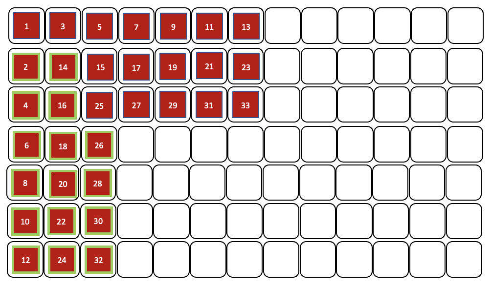
Figure 2: An example of a game in which the majority player $A$ uses the “cracking” strategy in Algorithm 2, at the point at which the bricks run out. The main idea of of the algorithm is that $A$ fills in as many columns as she can with bricks. Player $B$ may do anything. In this example, $B$ concentrates on winning one district at a time. The lower bound (Theorem 9) says that if the number of bricks $n<28$, then $B$ cannot win three districts. Here $n=33$, and $B$ just barely wins three districts. With $q=3,j=7,m=6$, we prove that $A$ can always fill $c=2$ columns, but in this example $A$ actually manages to fill $3$ columns.

Given $n$, find the largest value of $q$ such that $n<f(q)$, and use $q$ to find $c$;

In each round:;

if  no bricks remain then

     Play an apple to any open district;

      end if

     else if  there is any open district where the number of open spaces $<2(c-r)$, where $r$ is the number of bricks in the district then

          // Type a move

           Play a brick to that district ;

           end if

          else

               // Type b move

                Let $i$ be the least number of bricks in any open district;

                Play a brick to an open district containing $i$ bricks;

                end if

ALGORITHM 2 Strategy for the Majority Player

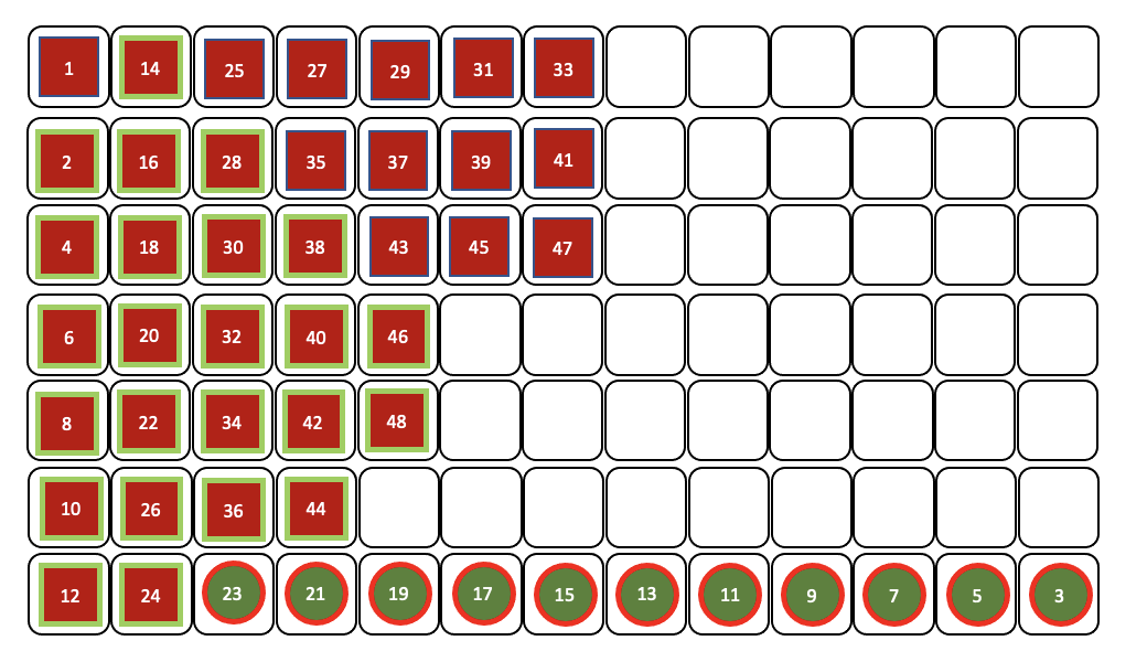
Figure 3: Another example game in which $A$ plays the “cracking” strategy, at the point at which the bricks run out. In this game $B$ fills in a row with apples so as to block $A$ from adding the final brick to columns 3 and 4, and then switches to winning districts one by one. Using the notation of Theorem 9, we have $j=7,m=6,q=3,c=2$, and $n=37$. We notice that $B$ needs $n=36$ to win three districts, while he only needed $33$ in Figure 2.

We will prove Theorem 9 using the strategy for $A$ that appears in Algorithm 2. In this strategy $A$ uses Theorem 9 to choose the smallest value of $q$ to which they can limit $B$. Using $q$, $A$ plays a classic “cracking” strategy in which they ensure that at least

$$c=\left\lfloor\frac{q}{j+q}(m+1)-\frac{1}{j+q}\right\rfloor$$

columns are filled with bricks at the end of the game. The Type a moves (see the algorithm) keep the first $c$ columns free of apples; this makes the analysis easier. Recall that an “open district” is one which contains fewer than $2m+1$ voters.

This strategy makes no sense unless $f(q)$ is monotone in $q$, so that a larger $q$ requires a larger $n$. Fortunately,

Observation 10.

If $q_{1}>q_{0}$, then $f(q_{1})>f(q_{0})$.

It also requires the following

Observation 11.

In any round, there is at most one district to which $A$ can make a move of type a.

This is because a move of type a is triggered by $B$ placing an apple into a district, reducing the number of open spaces $\omega$ to $2(c-r)-1$. The Type a move increases $r$, restoring $\omega=2(c-r)$. This gives us

Lemma 12.

If $A$ does not run out of bricks, there will be at least $c$ bricks in each district at the end of the game.

Now that we have established that the strategy makes sense, let’s proceed to
Proof of Theorem 9: Assume at the end of the game that $B$ has won $q$ districts.

The upper-left rectangle of size $q\times(m+1)$ contains only bricks. We claim that at least the first $c$ columns also contain only bricks. So assume for the purpose of contradiction that at most $c-1$ columns are filled with bricks.

In this case, we claim that every move by $A$ placed a brick into the first $c$ columns. This is always true for moves of type $a$, and because the first $c$ columns are not full, and cannot contain apples, it will be true of moves of type $b$ as well.

This means that all of the bricks outside of the first $c$ columns - of which there are at least $q(m+1-c)$ - must have been placed by $B$. To each of these moves, except possibly the last, $A$ responded by placing a brick into the first $c$ columns. It takes no more than $j$ bricks to fill a column, so it must be that $cj$ is strictly larger than the number of bricks in the first $c$ columns

$$cj > q(m+1-c)-1$$

$$c(j+q) > q(m+1)+1$$

$$c > \frac{q(m+1)}{j+q}-\frac{1}{j+q}$$

This contradicts the definition of $c$, so it must be the case that the first $c$ columns are filled with bricks.

So the total number of bricks must be

$$n \geq q(m+1)+(j-q)c$$

$$\geq q(m+1)+(j-q)\left\lfloor\frac{q}{j+q}(m+1)-\frac{1}{j+q}\right\rfloor$$

$$\geq q(m+1)+\frac{q(j-q)}{j+q}(m+1)-1$$

$$\geq q(m+1)+q(m+1)-\frac{2q^{2}}{j+q}(m+1)-1$$

$$\geq 2q\left(1-\frac{q}{j+q}\right)(m+1)-1$$

∎

7 Fairness Relative to Proportional Allocation

Theorem 9 describes the values of $n$ below which $B$ cannot win $q$ districts, and Theorem 8 describes the values of $n$ above which $B$ can always win at least $q$ districts. As a sanity check, we note that the range of $n$ where we do not know either that $B$ can or that $B$ cannot win $q$ districts is

$$2q(m+1)\geq n\geq 2q\left(1-\frac{q}{j+q}\right)(m+1)-1$$

and we see that this gap always exists.

Next, we recall that the proportional outcome is for $B$ to win $p$ districts, and that this implies that the number of bricks $n$ lies in a specific range:

$$(2p-1)m+p\leq n\leq(2p+1)m+p.$$

We consider the breakpoint values of $n$ at which $p$ changes. At the smallest value of $n$ at which the proportional representation is $p$, Theorem 8 tells us that $B$ can always win at least $p-1$ districts:

$$n=p+(2p-1)m\geq 2(p-1)(m+1)$$

Theorem 9 tells us that $B$ cannot win $p$ districts when $p$ is small:

$$n=p+(2p-1)m \leq 2p\left(1-\frac{p}{j+p}\right)(m+1)-1$$

$$2p(m+1)-m-p \leq 2p(m+1)-\frac{2p^{2}}{j+p}m-\frac{p}{j+p}-1$$

$$m+p \geq \frac{2p^{2}}{j+p}m+\frac{p}{j+p}+1$$

for instance, when $p<\sqrt{j}$.

8 Discussion

To visually compare the majority and minority players’ strategies, we graph an example for a game of reasonable size ($j=10$) in Figure 4.

Figure 4: The bounds illustrated for the case $j=10$. The $x$ axis is the number of bricks (voters of the minority party $B$) as a function of $m$, the size of a bare majority in a district. The $y$ axis is the number of districts that $B$ can win. The grey plot shows $p$, the number of districts $B$ wins if they are distributed proportionally. The red plot shows $n=\frac{2jq}{j+q}m$; Theorem 9 says that when $n$ is below this value, $B$ cannot win $q$ districts. The blue line shows $n=2qm$; Theorem 8 says that when $n$ is above this value, $B$ can always win $q$ districts.

We see that the gap between the lower bound (blue line) and upper bound (red line) on the number of minority voters $n$ required to win $q$ districts increases with $q$. We conjecture that improving the strategy for the minority player $B$ would show that $B$ can win more than $p$ districts when $n$ is large (although of course never more than $j/2$). That is, we conjecture that Redistricting Ghost favors the minority player when the minority is large, and the majority player when the minority is small. We further conjecture that these results depend only trivially on which player goes first.

It will be important to understand the results of Redistricting Ghost in more realistic settings, involving geometric and legal constraints on the districts. A good first step might be to analyze the protocol in a model that simplifies the distribution and geometry with a graph, as in [DeFord et al.(2019)].

Redistricting Ghost [Mixon and Villar(2018)], like I-cut-you-freeze [Pegden et al.(2017)] and the bisection protocol [Ludden et al.(2022)], does not allow the minority player to achieve proportional representation in the abstract setting when the minority is small. The fact that several protocols show the same effect suggests that it might be an inherent feature of the redistricting problem: there are many ways to “crack” a small group of minority voters and prevent them from dominating any one district. If this is inherent to the problem, one could consider this to be fair, that is, that small minorities should not expect to achieve proportional representation via redistricting, or perhaps it shows that the idea of electing representatives using districts, even independent of the geographic distribution of voters, is inherently unfair.

9 Acknowledgements

We thank an anonymous reviewer for pointing out an error in an earlier version of this paper. We thank (funding sources temporarily omitted) for support during this project.

References

- [1]
- [DeFord et al.(2019)] Daryl DeFord, Moon Duchin, and Justin Solomon. 2019. Recombination: A family of Markov chains for redistricting. arXiv preprint arXiv:1911.05725 31 (2019).
- [Dietrich(2021)] Eric Dietrich. 2021. How Montana got its new Congressional map. The Montana Free Press (2021). https://montanafreepress.org/2021/11/12/how-montanas-new-us-house-map-was-drawn
- [Imamura(2022)] David Imamura. 2022. The Rise and Fall of Redistricting Commissions: Lessons from the 2020 Redistricting Cycle. Human Rights Magazine 48, 1 (2022).
- [Landau and Su(2010)] Zeph Landau and Francis Edward Su. 2010. Fair Division and Redistricting. AMS Special Sessions on the Mathematics of Decisions, Elections, and Games pages 17-36 (2010).
- [Landau and Yershov(2009)] Zeph Landau and Reid I Yershov. 2009. A Fair Division Solution to the Problem of Redistricting. Social Choice and Welfare 32(3):479-492 (2009).
- [Ludden et al.(2022)] Ian G Ludden, Rahul Swamy, Douglas M King, and Sheldon H Jacobson. 2022. A bisection protocol for political redistricting. INFORMS Journal on Optimization (2022). https://rahulswamy.com/publications
- [Mixon and Villar(2018)] Dustin G Mixon and Soledad Villar. 2018. Utility Ghost: Gamified redistricting with partisan symmetry. arXiv preprint arXiv:1812.07377 (2018).
- [Pegden et al.(2017)] Wesley Pegden, Ariel D Procaccia, and Dingli Yu. 2017. A Partisan Districting Protocol with Provably Nonpartisan Outcomes. arXiv:1710.08781v1 (2017).
- [Pierce and Larson(2011)] Olga Pierce and Jeff Larson. 2011. How Democrats fooled California’s redistricting commission. ProPublica, Dec 21 (2011).
- [Stephanopoulos and McGhee(2014)] Nicholas Stephanopoulos and Eric McGhee. 2014. Partisan Gerrymandering and the Efficiency Gap. Public Law and Legal Theory Working Paper No. 493 (2014).
- [Tucker-Foltz(2019)] Jamie Tucker-Foltz. 2019. A Cut-And-Choose Mechanism to Prevent Gerrymandering. arXiv:1802.08351 [cs.GT] (2019).