Querying Easily Flip-flopped Samples
for Deep Active Learning

Abstract

Active learning is a machine learning paradigm that aims to improve the performance of a model by strategically selecting and querying unlabeled data. One effective selection strategy is to base it on the model’s predictive uncertainty, which can be interpreted as a measure of how informative a sample is. The sample’s distance to the decision boundary is a natural measure of predictive uncertainty, but it is often intractable to compute, especially for complex decision boundaries formed in multiclass classification tasks. To address this issue, this paper proposes the least disagree metric (LDM), defined as the smallest probability of disagreement of the predicted label, and an estimator for LDM proven to be asymptotically consistent under mild assumptions. The estimator is computationally efficient and can be easily implemented for deep learning models using parameter perturbation. The LDM-based active learning is performed by querying unlabeled data with the smallest LDM. Experimental results show that our LDM-based active learning algorithm obtains state-of-the-art overall performance on all considered datasets and deep architectures.

1 Introduction

Machine learning often involves the burdensome task of annotating a large unlabeled data set that is generally abundant and readily available. Active learning (Cohn et al., 1996) alleviates this burden by selecting the most informative unlabeled samples. Of the various active learning algorithms, uncertainty-based sampling (Ash et al., 2020; Zhao et al., 2021b; Woo, 2023) is preferred for its simplicity and relatively low computational cost. Uncertainty-based sampling selects unlabeled samples that are most difficult to predict (Settles, 2009; Yang et al., 2015; Sharma & Bilgic, 2017). The main focus of uncertainty-based sampling is quantifying the uncertainty of each unlabeled sample given a predictor. Until now, various uncertainty measures, as well as corresponding active learning algorithms, have been proposed (Nguyen et al., 2022; Houlsby et al., 2011; Jung et al., 2023); see Appendix A for a more comprehensive overview of the related work. However, many of them are not scalable or interpretable and often rely on heuristic approximations lacking theoretical justifications. This paper focuses on a conceptually simple approach based on the distance between samples and the decision boundary.

Indeed, the unlabeled samples closest to the decision boundary are considered the most uncertain samples (Kremer et al., 2014; Ducoffe & Precioso, 2018; Raj & Bach, 2022). It has been theoretically established that selecting unlabeled samples with the smallest margin leads to exponential performance improvement over random sampling in binary classification with linear separators (Balcan et al., 2007; Kpotufe et al., 2022). However, in most cases, the sample’s distance to the decision boundary is not computationally tractable, especially for deep neural network-based multiclass predictors. Various (approximate) measures have been proposed for identifying the closest samples to the decision boundary (Ducoffe & Precioso, 2018; Moosavi-Dezfooli et al., 2016; Mickisch et al., 2020), but most lack concrete justification.

This paper proposes a new paradigm of closeness measure that quantifies how easily sample prediction can be flip-flopped by a small perturbation in the decision boundary, departing from the conventional Euclidean-based distance. Therefore, samples identified to be closest by this measure are most uncertain in prediction and, thus, are the most informative. The main contributions of this paper are as follows:

• This paper defines the least disagree metric (LDM) as a measure of the sample’s closeness to the decision boundary.

• This paper proposes an estimator of LDM that is asymptotically consistent under mild assumptions and a simple algorithm to empirically evaluate the estimator, motivated from the theoretical analyses. The algorithm performs Gaussian perturbation centered around the hypothesis learned by stochastic gradient descent (SGD).

• This paper proposes an LDM-based active learning algorithm (LDM-S) that obtains state-of-the-art overall performance on six benchmark image datasets and three OpenML datasets, tested over various deep architectures.

2 Least Disagree Metric (LDM)

This section defines the least disagree metric (LDM) and proposes an asymptotically consistent estimator of LDM. Then, motivated from a Bayesian perspective, a practical algorithm for empirically evaluating the LDM is provided.

2.1 Definition of LDM

Let $\mathcal{X}$ and $\mathcal{Y}$ be the instance and label space with $|{\mathcal{Y}}|\geq 2$, and $\mathcal{H}$ be the hypothesis space of $h:\mathcal{X}\rightarrow\mathcal{Y}$. Let $\mathcal{D}$ be the joint distribution over $\mathcal{X}\times\mathcal{Y}$, and $\mathcal{D}_{\mathcal{X}}$ be the instance distribution. The LDM is inspired by the disagree metric defined by Hanneke (2014). The disagree metric between two hypotheses $h_{1}$ and $h_{2}$ is defined as follows:

$$\rho(h_{1},h_{2}):=\mathbb{P}_{X\sim\mathcal{D}_{\mathcal{X}}}[h_{1}(X)\neq h_{2}(X)]$$ (1)

where $\mathbb{P}_{X\sim\mathcal{D}_{\mathcal{X}}}$ is the probability measure on $\mathcal{X}$ induced by $\mathcal{D}_{\mathcal{X}}$. For a given hypothesis $g\in\mathcal{H}$ and ${\bm{x}}_{0}\in\mathcal{X}$, let $\mathcal{H}^{g,{\bm{x}}_{0}}:=\{h\in\mathcal{H}\mid h({\bm{x}}_{0})\neq g({\bm{x}}_{0})\}$ be the set of hypotheses disagreeing with $g$ in their prediction of ${\bm{x}}_{0}$. Based on the above set and disagree metric, the LDM of a sample to a given hypothesis is defined as follows:

Definition 1.

For given $g\in\mathcal{H}$ and ${\bm{x}}_{0}\in\mathcal{X}$, the least disagree metric (LDM) is defined as

$$L(g,{\bm{x}}_{0}):=\inf_{h\in\mathcal{H}^{g,{\bm{x}}_{0}}}\rho(h,g).$$ (2)

Throughout this paper , we will assume that all the hypotheses are parametric and the parameters that define the hypotheses $h$ and $g$ respectively are ${\bm{w}},{\bm{v}}\in{\mathbb{R}}^{p}$.

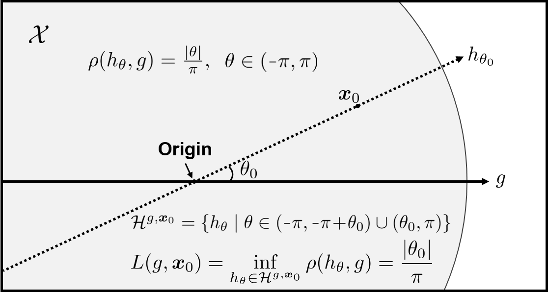
Figure 1: An example of LDM of ${\bm{x}}_{0}$ for given $g$ in binary classification with the linear classifier. Here ${\bm{x}}$ is uniformly distributed on $\mathcal{X}\subset\mathbb{R}^{2}$. The $h_{\theta}$ disagrees with $g$ for ${\bm{x}}_{0}$ when $\theta\!<\!\shortminus\pi\!+\!\theta_{0}$ or $\theta_{0}\!<\!\theta$, thus $L(g,{\bm{x}}_{0})\!=\!\inf_{h_{\theta}\in\mathcal{H}^{g,{\bm{x}}_{0}}}\rho(h_{\theta},g)=\frac{|\theta_{0}|}{\pi}$.

To illustrate the definition of LDM more clearly, we provide a simple example. Consider a two-dimensional binary classification with a set of linear classifiers,

$${\mathcal{H}}=\{h:h({\bm{x}})=\operatorname{sign}({\bm{x}}^{\mkern-1.5mu\mathsf{T}}{\bm{w}}),{\bm{w}}\in{\mathbb{R}}^{2}\}$$

where ${\bm{x}}$ is uniformly distributed on ${\mathcal{X}}=\{{\bm{x}}:\|{\bm{x}}\|\leq 1\}\subset{\mathbb{R}}^{2}$. Let $h_{\theta}$ be a hypothesis leading to decision boundary that forms an angle (radian) of $\theta\in(\shortminus\pi,\pi)$ with that of $g$, then we have that $\rho(h_{\theta},g)=\frac{|\theta|}{\pi}$. For given $g$ and ${\bm{x}}_{0}$, let $\theta_{0}\in(0,\frac{\pi}{2})$ be the angle between the decision boundary of $g$ and the line passing through ${\bm{x}}_{0}$, then $\mathcal{H}^{g,{\bm{x}}_{0}}=\{h_{\theta}\mid\theta\in(\shortminus\pi,\shortminus\pi\!+\!\theta_{0})\cup(\theta_{0},\pi)\}$; see Figure 1. Thus, $L(g,{\bm{x}}_{0})=\inf_{h_{\theta}\in\mathcal{H}^{g,{\bm{x}}_{0}}}\rho(h_{\theta},g)=\frac{|\theta_{0}|}{\pi}$.

Conceptually, a sample with a small LDM indicates that its prediction can be easily flip-flopped even by a small perturbation in the predictor. Precisely, suppose that a hypothesis $h$ is sampled with its parameter given by ${\bm{w}}\sim\mathcal{N}({\bm{v}},\mathbf{I}\sigma^{2})$, then it is expected that

$$L(g,{\bm{x}}_{1})<L(g,{\bm{x}}_{2})\Leftrightarrow\mathbb{P}_{\bm{w}}[h({\bm{x}}_{1})\neq g({\bm{x}}_{1})]>\mathbb{P}_{\bm{w}}[h({\bm{x}}_{2})\neq g({\bm{x}}_{2})].$$

The sample with the smallest LDM is the most uncertain and, thus, most informative. This intuition is rigorously verified for the two-dimensional binary classification with linear classifiers and is empirically verified on benchmark datasets with deep networks (see Appendix C.1).

2.2 An Asymptotically Consistent Estimator of LDM

In most cases, LDM is not computable for the following two reasons: 1) $\rho$ is generally intractable, especially when $\mathcal{D}_{\mathcal{X}}$ and $h$ are both complicated, e.g., neural networks over real-world image datasets, and 2) one needs to take an infimum over $\mathcal{H}$, which is usually an infinite set.

To address these issues, we propose an estimator for the LDM based on the following two approximations: 1) $\mathbb{P}$ in the definition of $\rho$ is replaced by an empirical probability based on $M$ samples (Monte-Carlo method), and 2) ${\mathcal{H}}$ is replaced by a finite hypothesis set ${\mathcal{H}}_{N}$ of cardinality $N$. Our estimator, denoted by $L_{N,M}(g,\bm{x}_{0})$, is defined as follows:

$$L_{N,M}(g,\bm{x}_{0}):=\inf_{h\in\mathcal{H}_{N}^{g,\bm{x}_{0}}}\left\{\rho_{{}_{M}}(h,g)\triangleq\frac{1}{M}\sum_{i=1}^{M}\mathbb{I}\big{[}h(X_{i})\neq g(X_{i})\big{]}\right\},$$ (3)

where $\mathcal{H}_{N}^{g,\bm{x}_{0}}:=\left\{h\in{\mathcal{H}}_{N}\mid h\in{\mathcal{H}}^{g,{\bm{x}}_{0}}\right\}$, $\mathbb{I}[\cdot]$ is an indicator function, and $X_{1},\ldots,X_{M}\overset{i.i.d.}{\sim}{\mathcal{D}}_{\mathcal{X}}$. Here, $M$ is the number of Monte Carlo samples for approximating $\rho$, and $N$ is the number of sampled hypotheses for approximating $L$.

One important property of an estimator is (asymptotic) consistency, i.e., in our case, we want the LDM estimator to converge in probability to the true LDM as $M$ and $N$ increase indefinitely.

We start with two assumptions on the hypothesis space ${\mathcal{H}}$ and the disagree metric $\rho$:

Assumption 1.

${\mathcal{H}}$ is a Polish space with metric $d_{\mathcal{H}}(\cdot,\cdot)$.

This assumption allows us to avoid any complications that may arise from uncountability, especially as we will consider a probability measure over $\mathcal{H}$; see Chapter 1.1 of van der Vaart & Wellner (1996).

Assumption 2.

$\rho(\cdot,\cdot)$ is $B$-Lipschitz for some $B>0$, i.e., $\rho(h,g)\leq Bd_{\mathcal{H}}(h,g),\ \forall h,g\in{\mathcal{H}}$.

If $\rho$ is not Lipschitz, then the disagree metric may behave arbitrarily regardless of whether the hypotheses are “close” or not. This can occur in specific (arguably not so realistic) corner cases, such as when ${\mathcal{D}}_{\mathcal{X}}$ is a mixture of Dirac measures.

From hereon and forth, we fix some $g\in{\mathcal{D}}$ and ${\bm{x}}_{0}\in{\mathcal{X}}$.

The following assumption intuitively states that ${\mathcal{H}}_{N}$ is more likely to cover regions of ${\mathcal{H}}$ whose LDM estimator is $\varepsilon$-close to the true LDM, as the number of sampled hypotheses $N$ increases.

Assumption 3 (Coverage Assumption).

There exist two deterministic functions $\alpha:{\mathbb{N}}\times{\mathbb{R}}_{\geq 0}\rightarrow{\mathbb{R}}_{\geq 0}$ and $\beta:{\mathbb{N}}\rightarrow{\mathbb{R}}_{>0}$ that satisfies $\lim_{N\rightarrow\infty}\alpha(N,\varepsilon)=\lim_{N\rightarrow\infty}\beta(N)=0$ for any $\varepsilon\in(0,1)$, and

$${\mathbb{P}}\left[\inf_{\begin{subarray}{c}h^{*}\in{\mathcal{H}}^{g,{\bm{x}}_{0}}\\ \rho(h^{*},g)-L(g,{\bm{x}}_{0})\leq\varepsilon\end{subarray}}\min_{h\in{\mathcal{H}}_{N}^{g,{\bm{x}}_{0}}}d_{\mathcal{H}}(h^{*},h)\leq\frac{1}{B}\alpha(N,\varepsilon)\right]\geq 1-\beta(N),\quad\forall\varepsilon\in(0,1),$$ (4)

where we recall that ${\mathcal{H}}^{g,{\bm{x}}_{0}}=\{h\in{\mathcal{H}}\mid h({\bm{x}}_{0})\neq g({\bm{x}}_{0})\}$.

Here, we implicitly assume that there is a randomized procedure that outputs a sequence of finite sets ${\mathcal{H}}_{1}\subseteq{\mathcal{H}}_{2}\subseteq\cdots\subset{\mathcal{H}}$. $\alpha(N,\varepsilon)$ is the rate describing the optimality of approximating ${\mathcal{H}}$ using ${\mathcal{H}}_{N}$ in that how close is the $\varepsilon$-optimal solution is, and $1-\beta(N)$ is the confidence level that converges to $1$.

In the following theorem, whose proof is deferred to Appendix B, we show that our proposed estimator, $L_{N,M}$, is asymptotically consistent:

Theorem 1.

Let $g\in{\mathcal{H}}$, ${\bm{x}}_{0}\in{\mathcal{X}}$, and $\delta>0$ be arbitrary. Under Assumption 1, 2, and 3, with $M>\frac{8}{\delta^{2}}\log(CN)$, we have that for any $\varepsilon\in(0,1)$,

$${\mathbb{P}}\left[\left|L_{N,M}(g,\bm{x}_{0})-L(g,\bm{x}_{0})\right|\leq 2\delta+\alpha(N,\varepsilon)+\varepsilon\right]\geq 1-\frac{1}{CN}-\beta(N).$$

Furthermore, as $\min(M,N)\rightarrow\infty$ with $M=\omega\left(\log(CN)\right)$, we have $L_{N,M}(g,\bm{x}_{0})\overset{{\mathbb{P}}}{\rightarrow}L(g,\bm{x}_{0}).$

For our asymptotic guarantee, we require $M=\omega(\log(CN))$, while the guarantee holds w.p. at least $1-\frac{1}{CN}-\beta(N)$. For instance, when $\beta(N)$ scales as $1/N$, the above implies that when $N$ scales exponentially (in dimension or some other quantity), the guarantee holds with overwhelming probability while $M$ only needs to be at least scaling linearly, i.e., $M$ needs not be too large.

One important consequence is that the ordering of the empirical LDM is preserved in probability:

Corollary 1.

Assume that $L(g,\bm{x}_{i})<L(g,\bm{x}_{j})$. Under the same assumptions as Theorem 1, the following holds: for any $\varepsilon>0$,

$$\lim_{\begin{subarray}{c}\min(M,N)\rightarrow\infty\\ M=\omega(\log(CN))\end{subarray}}{\mathbb{P}}\left[L_{N,M}(g,\bm{x}_{i})>L_{N,M}(g,\bm{x}_{j})+\varepsilon\right]=0.$$

2.3 Empirical Evaluation of LDM

Motivation.

Assumption 3 must be satisfied for our LDM estimator to be asymptotically consistent, as only then could we hope to “cover” the hypothesis that yields the true LDM with high probability as $N\rightarrow\infty$. To do that, we consider Gaussian sampling around the target hypothesis $g$ to construct a sufficiently large, finite collection of $N$ hypotheses $\mathcal{H}_{N}$. Indeed, we show in Appendix C.3 that this is the case for 2D binary classification with linear classifiers.

Remark 1.

It is known that SGD performs Bayesian inference (Mandt et al., 2017; Chaudhari & Soatto, 2018; Mingard et al., 2021), i.e., $g$ can be thought of as a sample from a posterior distribution. Combined with the Bernstein-von Mises theorem (Hjort et al., 2010), which states that the posterior of a parametric model converges to a normal distribution under mild conditions, Gaussian sampling around $g$ can be thought of as sampling from a posterior distribution, in an informal sense.

Algorithm Details.

Algorithm 1 empirically evaluates the LDM of ${\bm{x}}$ for given $g$. When sampling the hypotheses, we use a set of variances $\{\sigma_{k}^{2}\}_{k=1}^{K}$ such that $\sigma_{k}<\sigma_{k+1}$. The reason for this is two-fold. First, with too small $\sigma^{2}$, the sampled hypothesis $h$ is expected to not satisfy $h({\bm{x}})\neq g({\bm{x}})$. On the other hand, it may be that with too large $\sigma^{2}$, the minimum of $\rho_{{}_{M}}(h,g)$ over the sampled $h$’s is too far away from the true LDM, especially when the true LDM is close to $0$. Both reasons are based on the intuition that larger $\sigma^{2}$ implies that the sampled hypothesis $h$ is further away from $g$. In Appendix C.2, we prove that $\mathbb{E}_{{\bm{w}}}[\rho_{{}_{M}}(h,g)]$ is monotone increasing in $\sigma^{2}$ for 2D binary classification with linear classifiers, and also show empirically that this holds for more realistic scenarios. The algorithm proceeds as follows: for each $k$, $h$ is sampled with ${\bm{w}}\sim\mathcal{N}({\bm{v}},\mathbf{I}\sigma_{k}^{2})$, and if $h({\bm{x}})\neq g({\bm{x}})$ then update $L_{{\bm{x}}}$ as $\min\{L_{{\bm{x}}},\rho_{{}_{M}}(h,g)\}$. When $L_{{\bm{x}}}$ does not change $s$ times consecutively, move on to $k+1$. This is continued while $k<K$.

Small $s$ is Sufficient.

The remaining question is how to determine an appropriate $s$. In binary classification with the linear classifier described in Figure 1, the evaluated LDM reaches the true LDM even with a small $s$. However, a large $s$ is required for deep architectures to make the evaluated LDM converge. This is computationally prohibitive as the evaluation requires a huge runtime for sampling a large number of hypotheses. Fortunately, we observed empirically that for all considered values of $s$, the rank order of samples’ LDMs is preserved with a high rank-correlation coefficient close to $1$. As the ordering induced by the LDMs is enough for the LDM-based active learning (described in Section 3), a small $s$ is sufficient. Experimental details and further discussions on the stop condition $s$ are deferred to Appendix F.1.

3 LDM-based Active Learning

This section introduces LDM-S, the LDM-based batch sampling algorithm for pool-based active learning. In pool-based active learning, we have a set of unlabeled samples, $\mathcal{U}$, and we simultaneously query $q$ samples from randomly sampled pool data $\mathcal{P}\subset\mathcal{U}$ of size $m$. In our algorithm, a given hypothesis $g$ is obtained by training on labeled samples, and $\bm{v}$ is the parameter of $g$.

Algorithm 1 Empirical Evaluation of LDM

  Input: $\bm{x}$: target sample $g$: target hypothesis parameterized by ${\bm{v}}$ $M$: number of samples for approximation $\{\sigma_{k}^{2}\}_{k=1}^{K}$: set of variances$s$: stop condition for parameter sampling

  

  $L_{{\bm{x}}}=1$

  for $k=1$ to $K$ do

     $c=0$

     while $c<s$ do

        Sample $h$ with ${\bm{w}}\sim\mathcal{N}({\bm{v}},\mathbf{I}\sigma_{k}^{2})$

        $c=c+1$

        if $h({\bm{x}})\neq g({\bm{x}})$ and $L_{{\bm{x}}}>\rho_{{}_{M}}(h,g)$ then

           $L_{{\bm{x}}}\leftarrow\rho_{{}_{M}}(h,g)$

           $c=0$

        end if

     end while

  end for

  return: $L_{{\bm{x}}}$

Algorithm 2 Active Learning with LDM-S

  Input: $\mathcal{L}_{0},\mathcal{U}_{0}$ : Initial labeled and unlabeled samples$m,q$ : pool and query size$T$ : number of acquisition steps

  

  for $t=0$ to $T-1$ do

     Obtain ${\bm{v}}$ by training on $\mathcal{L}_{t}$

     Randomly sample $\mathcal{P}\subset\mathcal{U}_{t}$ with $|\mathcal{P}|=m$

     Evaluate $L_{{\bm{x}}}$ of ${\bm{x}}\in\mathcal{P}$ for ${\bm{v}}$ by Algorithm 1

     Compute $\gamma({\bm{x}})$ using Eqn. 5

     $\mathcal{Q}_{1}\leftarrow\{{\bm{x}}_{1}\}$ where ${\bm{x}}_{1}=\operatorname*{arg\,min}_{{\bm{x}}\in\mathcal{P}}L_{{\bm{x}}}$

     for $n=2$ to $q$ do

        $p({\bm{x}})=\gamma({\bm{x}})*\min_{{\bm{x}}^{\prime}\in\mathcal{Q}_{n-1}}d_{\cos}(\bm{z}_{{\bm{x}}},\bm{z}_{{\bm{x}}^{\prime}})$

        Sample ${\bm{x}}_{n}\in\mathcal{P}$ w.p. $\mathbb{P}({\bm{x}}_{n})=\frac{p({\bm{x}}_{n})^{2}}{\sum_{{\bm{x}}_{j}\in\mathcal{P}}p({\bm{x}}_{j})^{2}}$

        $\mathcal{Q}_{n}\leftarrow\mathcal{Q}_{n-1}\cup\{{\bm{x}}_{n}\}$

     end for

     $\mathcal{L}_{t+1}\leftarrow\mathcal{L}_{t}\cup\{({\bm{x}}_{i},y_{i})\}_{{\bm{x}}_{i}\in\mathcal{Q}_{q}},\ \mathcal{U}_{t+1}\leftarrow\mathcal{U}_{t}\setminus\mathcal{Q}_{q}$

  end for

3.1 LDM-Seeding

One naïve approach to active learning with LDM is to select $q$ samples with the smallest LDMs, i.e., most uncertain samples. However, as shown in Appendix C.4, this algorithm may not lead to good performance. Upon further inspection, we observe cases where there is a significant overlap of information in the selected batches, and samples with larger LDMs are more helpful. This issue, often referred to as sampling bias, is prevalent in uncertainty-based active learning (Dasgupta, 2011). One popular approach to mitigate this is considering diversity, which has been done via $k$-means++ seeding (Ash et al., 2020), submodular maximization (Wei et al., 2015), clustering (Citovsky et al., 2021; Yang et al., 2021), joint mutual information (Kirsch et al., 2019), and more.

This paper incorporates diversity via a modification of the $k$-means++ seeding algorithm (Arthur & Vassilvitskii, 2007), which is effective at increasing batch diversity without introducing additional hyperparameters (Ash et al., 2020). Intuitively, the $k$-means++ seeding selects centroids by iteratively sampling points proportional to their squared distance from the nearest centroid that has already been chosen, which tends to select a diverse batch. Our proposed modification uses the cosine distance between the last layer features of the deep network, motivated by the fact that the perturbation is applied to the weights of the last layer, and the scales of features do not matter in the final prediction.

We introduce the seeding methods based on the principle of querying samples with the smallest LDMs while pursuing diversity. For querying samples with the smallest LDMs, this paper considers a modified exponentially decaying weighting with respect to LDM in an EXP3-type manner (Auer et al., 2002); such weighting scheme has been successfully applied to active learning (Beygelzimer et al., 2009; Ganti & Gray, 2012; Kim & Yoo, 2022). To balance selecting samples with the smallest LDMs versus increasing diversity, $\mathcal{P}$ is partitioned as $\mathcal{P}_{q}$ and $\mathcal{P}_{c}$, then the total weights of $\mathcal{P}_{q}$ and $\mathcal{P}_{c}$ are set to be equal, where $\mathcal{P}_{q}$ is the set of samples with smallest LDM of size $q$ (=query size) and $\mathcal{P}_{c}=\mathcal{P}\setminus\mathcal{P}_{q}$. Precisely, the weights of ${\bm{x}}\in\mathcal{P}$ are defined as follows: for each ${\bm{x}}\in{\mathcal{P}}_{i}$,

$$\gamma({\bm{x}})=\frac{\exp\left(-\frac{(L_{{\bm{x}}}-L_{q})_{+}}{L_{q}}\right)}{\sum_{{\bm{x}}\in{\mathcal{P}}_{i}}\exp\left(-\frac{(L_{{\bm{x}}}-L_{q})_{+}}{L_{q}}\right)},$$ (5)

where $i\in\{q,c\}$ is the indices of the partition of ${\mathcal{P}}$, $(\cdot)_{+}=\max\{0,\cdot\}$, and $L_{q}=\max_{{\bm{x}}\in\mathcal{P}_{q}}L_{{\bm{x}}}$.

LDM-Seeding starts by selecting an unlabeled sample with the smallest LDM in $\mathcal{P}$. The next distinct unlabeled sample is sampled from $\mathcal{P}$ by the following probability:

$$\mathbb{P}({\bm{x}})=\frac{p({\bm{x}})^{2}}{\sum_{{\bm{x}}_{j}\in\mathcal{P}}p({\bm{x}}_{j})^{2}},\quad p({\bm{x}})=\gamma({\bm{x}})*\min_{{\bm{x}}^{\prime}\in\mathcal{Q}}d_{\cos}(\bm{z}_{{\bm{x}}},\bm{z}_{{\bm{x}}^{\prime}})$$ (6)

where $Q$ is the set of selected samples, and ${\bm{z}}_{{\bm{x}}},{\bm{z}}_{{\bm{x}}^{\prime}}$ are the features of ${\bm{x}},{\bm{x}}^{\prime}$. Note that the selection probability is explicitly impacted by LDMs while having diversity. The effectiveness of LDM is shown in Figure 12 of Section 4.1.

3.2 LDM-S: Active Learning with LDM-Seeding

We now introduce LDM-S in Algorithm 2, the LDM-based seeding algorithm for active learning. Let $\mathcal{L}_{t}$ and $\mathcal{U}_{t}$ be the set of labeled and unlabeled samples at step $t$, respectively. For each step $t$, the given parameter $\bm{v}$ is obtained by training on $\mathcal{L}_{t}$, and the pool data $\mathcal{P}\subset\mathcal{U}_{t}$ of size $m$ is drawn uniformly at random. Then for each ${\bm{x}}\in\mathcal{P}$, $L_{{\bm{x}}}$ for given ${\bm{v}}$ and $\gamma({\bm{x}})$ are evaluated by Algorithm 1 and Eqn. 5, respectively. The set of selected unlabeled samples, $\mathcal{Q}_{1}$, is initialized as $\{{\bm{x}}_{1}\}$ where ${\bm{x}}_{1}=\operatorname*{arg\,min}_{{\bm{x}}\in\mathcal{P}}L_{{\bm{x}}}$. For $n=2,\ldots,q$, the algorithm samples ${\bm{x}}_{n}\in\mathcal{P}$ with probability $\mathbb{P}({\bm{x}})$ in Eqn. 6 and appends it to $\mathcal{Q}_{n}$. Lastly, the algorithm queries the label $y_{i}$ of each ${\bm{x}}_{i}\in\mathcal{Q}_{q}$, and the algorithm continues until $t=T-1$.

4 Experiments

This section presents the empirical results of the effectiveness of LDM in the proposed algorithm, as well as a comprehensive performance comparison with various uncertainty-based active learning algorithms. We evaluate our approach on three OpenML (OML) datasets (#6 (Frey & Slate, 1991), #156 (Vanschoren et al., 2014), and #44135 (Fanty & Cole, 1990)) and six benchmark image datasets (MNIST (Lecun et al., 1998), CIFAR10 (Krizhevsky, 2009), SVHN (Netzer et al., 2011), CIFAR100 (Krizhevsky, 2009), Tiny ImageNet (Le & Yang, 2015), FOOD101 (Bossard et al., 2014)), and ImageNet (Russakovsky et al., 2015). MLP, S-CNN, K-CNN (Chollet et al., 2015), Wide-ResNet (WRN-16-8; (Zagoruyko & Komodakis, 2016)), and ResNet-18 (He et al., 2016) are used to evaluate the performance. All results are averaged over $5$ repetitions ($3$ for ImageNet). Precise details for datasets, architectures, and experimental settings are presented in Appendix D.

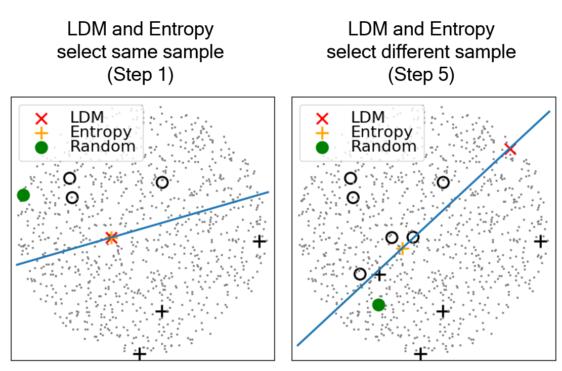
(a)

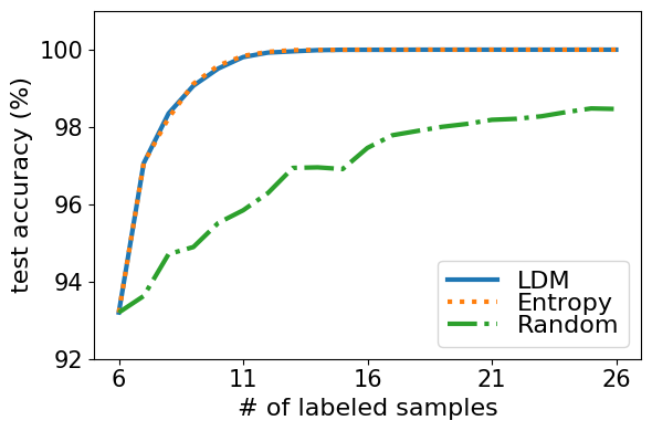
(b)

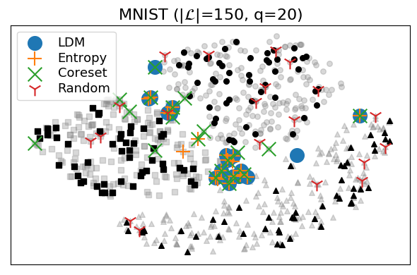
(c)

Figure 2: The comparison of selecting sample(s). The black crosses and circles are labeled, and the gray dots are unlabeled samples. (a) Samples selected by LDM-based, entropy-based, and random sampling in binary classification with the linear classifier. (b) The test accuracy with respect to the number of labeled samples. (c) The t-SNE plot of selected batch samples in 3-class classification with a deep network on MNIST dataset.

4.1 Effectiveness of LDM in Selecting (Batched) Uncertain Samples

To investigate how LDM works, we conduct a simple active learning experiment in a setting where true LDM is measurable. We consider two-dimensional binary classification with $\mathcal{H}=\{h:h_{\bm{w}}({\bm{x}})={\mathbb{I}}[\ell_{\bm{w}}({\bm{x}})>0.5]\}$ where $\ell_{\bm{w}}({\bm{x}}):=1/(1+e^{-(\bm{x}^{\mkern-1.5mu\mathsf{T}}\bm{w})})$ and $\bm{w}\in\mathbb{R}^{2}$ is the parameter of $h$ and $\bm{x}$ is uniformly distributed on $\mathcal{X}=\{\bm{x}:\|\bm{x}\|\leq 1\}\subset\mathbb{R}^{2}$. Three initial labeled samples are randomly selected from each class, and one sample is queried at each step. LDM-based active learning (LDM) is compared with entropy-based uncertainty sampling (Entropy) and random sampling (Random). Figure 2a shows examples of the samples selected by each algorithm. The black crosses and circles are labeled samples, and the gray dots are unlabeled. Both LDM and Entropy select samples close to the decision boundary. Figure 2b shows the average test accuracy of 100 replicates with respect to the number of labeled samples. LDM performs like Entropy, which is much better than Random. In binary classification, entropy is a strongly decreasing function of the distance to the decision boundary. That is, the entropy-based algorithm selects the sample closest to the decision boundary in the same way as the margin-based algorithm, and the effectiveness of this method has been well-proven theoretically and empirically in binary classification. We also compared the batch samples selected by LDM, Entropy, Coreset, and Random in 3-class classification with a deep network on the MNIST dataset. Figure 2c shows the t-SNE plot of the selected batch samples. The gray and black points are pool data and labeled samples, respectively. The results show that LDM and Entropy select samples close to the decision boundary, while Coreset selects more diverse samples. For further ablations, we’ve considered varying batch sizes (Appendix F.3), seeding algorithms without use of LDM (Appendix F.2), and vanilla seeding algorithm with other uncertainty measures (Appendix G.1), all of which show the effectiveness of our newly introduced LDM.

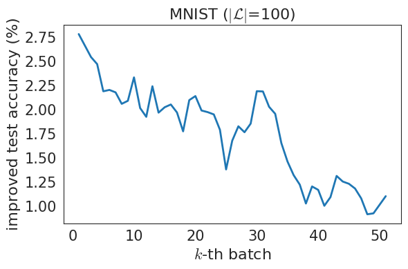
(a)

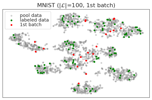
(b)

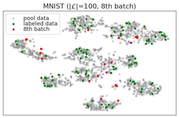
(c)

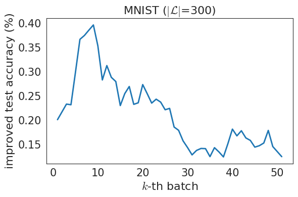
(d)

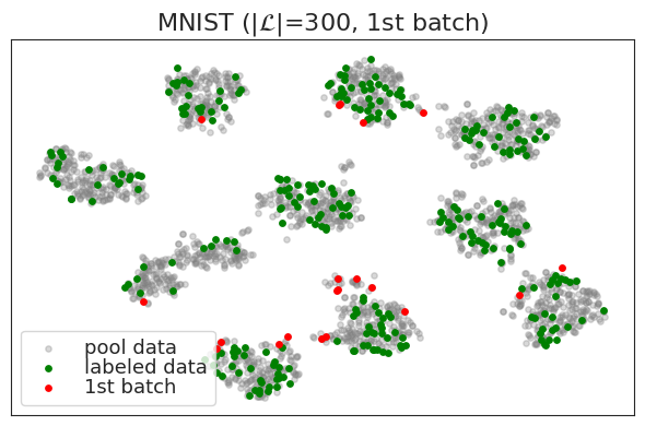
(e)

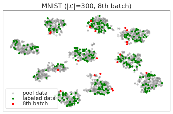
(f)

Figure 3: The improved test accuracy by labeling the $k$^th batch of size $q$ from pool data sorted in ascending order of LDM when the number of labeled samples is $100$ (a) or $300$ (d), and t-SNE plots of the first and eighth batches for each case (b-c, e-f) on MNIST.

4.2 Necessity of Pursuing Diversity in LDM-S

Here, we provide ablations on the effect of diverse sampling (and why we need to consider diversity) by considering the scenario in which we query samples with the smallest LDMs only We query the $k$^th batch of size $q=20$ for $k\in[50]$ from MNIST sorted in ascending order of LDM and compare the improvements in test accuracy. As shown in Figure 3a where $100$ samples are labeled, samples with the smallest LDMs lead to the best performance, whereas in Figure 3d where $300$ samples are labeled, that is not the case. To see why this is the case, we’ve plotted the t-SNE plots (van der Maaten & Hinton, 2008) of the first and eighth batches for each case. In the first case, as shown in Figure 3b–3c, the samples of the first and eighth batches are all spread out, so there is no overlap of information between the samples in each batch; taking a closer look, it seems that smaller LDM leads to the samples being more spread out. However, in the second case, as shown in Figure 3e–3f, the samples of the first batch are close to one another, i.e., there is a significant overlap of information between the samples in that batch. Surprisingly, this is not the case for the eighth batch, which consists of samples of larger LDMs. This leads us to conclude that diversity should be considered in the batch selection setting, even when using the LDM-based approach. In Appendix C.4, we provide a geometrical intuition of this phenomenon in 2D binary classification with linear classifiers.

4.3 Comparing LDM-S to Baseline Algorithms

We now compare the performance of LDM-S with the baseline algorithms. We first describe the baseline algorithms we compare, then provide comparisons across and per the considered datasets.

Baseline algorithms

Each baseline algorithm is denoted as follows: ‘Rand’: random sampling, ‘Entropy’: entropy-based uncertainty sampling (Shannon, 1948), ‘Margin’: margin-based sampling (Roth & Small, 2006), ‘Coreset’: core-set selection (Sener & Savarese, 2018), ‘ProbCov’: maximizing probability coverage (Yehuda et al., 2022), ‘DBAL’: MC-dropout sampling with BALD (Gal et al., 2017), ‘ENS’: ensemble method with variation ratio (Beluch et al., 2018), ‘BADGE’: batch active learning by diverse gradient embeddings (Ash et al., 2020), and ‘BAIT’: batch active learning via information metrics (Ash et al., 2021). For DBAL, we use $100$ forward passes for MC-dropout, and for ENS, we use an ensemble consisting of $5$ identical but randomly initialized networks. DBAL can not be conducted on ResNet-18, and BAIT can not be conducted with our resources on CIFAR100, Tiny ImageNet, FOOD101, and ImageNet since it requires hundreds to thousands of times longer than CIFAR10. For the hyperparameters of our LDM-S, we set $s=10$, $M$ to be the same size as the pool size, and $\sigma_{k}=10^{\beta k-5}$ where $\beta=0.1$ and $k\in\{1,2,\cdots,51\}$ in convenient (see Appendix F.4).

Performance comparison across datasets

It isn’t easy to find an algorithm that performs best in all benchmark datasets, but there is a clear winner that performs best on average on the nine benchmark datasets considered in the paper. The performance profile (Dolan & Moré, 2002) and penalty matrix (Ash et al., 2020) are examined to provide comprehensive comparisons across datasets. The details of the performance profile and penalty matrix are described in Appendix E. Figure 4a shows the performance profile w.r.t. $\delta$. Overall, it is clear that LDM-S retains the highest $R_{A}(\delta)$ over all considered $\delta$’s. We also observe that $R_{\text{LDM-S}}(0)=35\%$ while the other algorithms have a value less than $15\%$. This clearly shows that our LDM-S outperforms the other considered algorithms. Figure 4b shows the resulting penalty matrix. First, note that in the first row, LDM-S outperforms all the other algorithms up to statistical significance, sometimes more than half the time. (Recall that the largest entry of the penalty matrix is, at most, $9$, the total number of datasets.) Also, looking at the first column, it is clear that no other algorithm beats LDM-S over all runs. Looking at the bottom row, it is clear that LDM-S obtains the best overall performance.

Table 1: The mean $\pm$ standard deviation of the repetition-wise averaged performance (test accuracy) differences (%), relative to Random, over the entire steps. The positive value indicates higher performance than Random, and the asterisk (^∗) indicates that $p<0.05$ in paired sample $t$-test between LDM-S and others. (bold+underlined: best performance, bold: second-best performance)

	LDM-S (ours)	Entropy (1948)	Margin (2006)	Coreset (2018)	ProbCov (2022)	DBAL (2017)	ENS (2018)	BADGE (2020)	BAIT (2021)
OML#6	4.76±0.36	-2.46±0.70*	4.11±0.24	1.14±0.33*	0.19±0.40*	0.10±0.22*	4.43±0.31	2.98±0.28*	2.57±0.30*
OML#156	1.18±0.32	-1.29±0.51*	0.64±0.39*	-19.53±3.32*	-0.08±0.51*	-14.40±1.08*	0.61±0.35*	1.06±0.39	-7.66±1.12*
OML#44135	4.36±0.27	1.84±0.36*	4.11±0.32	0.27±0.68*	3.55±0.28*	1.61±0.45*	2.47±0.37*	2.48±0.44*	2.55±0.41*
MNIST	3.33±0.43	2.36±0.84*	3.01±0.45	-0.04±1.23*	2.92±0.41	1.68±0.80*	2.98±0.36	3.01±0.45	3.37±0.43
CIFAR10	1.34±0.19	0.00±0.21*	0.43±0.27*	-3.71±0.56*	0.04±0.37*	-0.15±0.31*	0.58±0.28*	0.90±0.21*	0.60±0.13*
SVHN	2.53±0.22	1.52±0.19*	1.98±0.18*	-1.66±0.51*	0.88±0.14*	2.46±0.21	2.08±0.22*	2.18±0.23*	2.18±0.23*
CIFAR100	0.98±0.44	0.37±0.60	0.57±0.45	0.89±0.49	0.74±0.60	0.55±0.77	0.03±0.41*	0.64±0.48	-
T. ImageNet	0.55±0.16	-0.61±0.28*	0.28±0.29	-0.20±0.46*	0.45±0.23	0.27±0.19*	-0.15±0.35*	0.12±0.40*	-
FOOD101	1.27±0.34	-0.86±0.20*	0.34±0.25*	1.30±0.16	0.50±0.22*	1.18±0.35	-0.15±0.46*	0.71±0.43*	-
ImageNet	0.96±0.23	-0.21±0.58*	0.14±0.54	-0.62±0.20*	0.30±0.22*	-	0.57±0.21	0.71±0.81	-

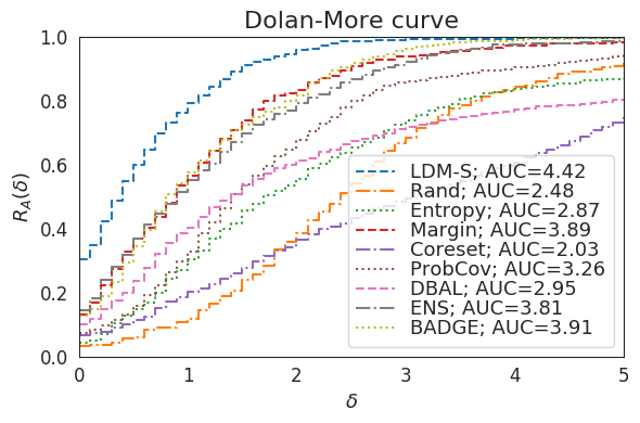
(a)

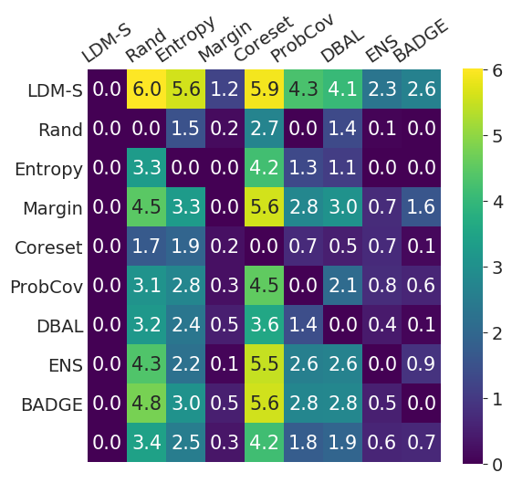
(b)

Figure 4: The performance comparison across datasets (a) Dolan-Moré plot among the algorithms across all experiments. AUC is the area under the curve. (b) The pairwise penalty matrix over all experiments. Element $P_{i,j}$ corresponds roughly to the number of times algorithm $i$ outperforms algorithm $j$. Column-wise averages at the bottom show overall performance (lower is better).

Table 2: The mean of runtime (min) for each algorithm and each dataset. We observe that LDM-S operates as fast as Entropy on almost all datasets.

	LDM-S	Entropy	Margin	Coreset	ProbCov	DBAL	ENS	BADGE	BAIT
OML#6	7.1	6.0	5.9	6.4	5.8	5.8	28.1	6.2	628.8
OML#156	4.5	4.2	3.7	4.4	4.0	4.2	17.5	4.2	60.2
OML#44135	5.2	4.0	4.6	4.2	6.2	4.2	18.2	4.4	319.8
MNIST	17.6	10.4	11.3	11.3	10.4	12.1	49.6	12.5	27.9
CIFAR10	106.0	99.6	101.0	106.1	97.5	108.0	496.0	102.2	6,436.5
SVHN	68.9	65.1	66.6	70.9	64.8	105.8	324.8	70.5	6,391.6
CIFAR100	405.9	395.2	391.4	429.7	405.5	447.8	1,952.1	445.3	-
T. ImageNet	4,609.5	4,465.9	4,466.1	4,706.8	4,621.4	4,829.2	19,356.4	5,152.5	-
FOOD101	4,464.8	4,339.8	4,350.3	4,475.7	4,471.0	4,726.8	18,903.3	4,703.9	-

Performance comparison per datatset

Table 1 presents the mean and standard deviation of the repetition-wise averaged performance differences, relative to Random, over the entire steps. The positive value indicates higher performance compared to Random, and the asterisk (^∗) indicates the $p$-value is less than 0.05 in paired sample $t$-test for the null of no difference versus the alternative that the LDM-S is better than each of the compared algorithm. We observe that LDM-S either consistently performs best or is comparable with other algorithms for all datasets. In contrast, the performance of the algorithms except LDM-S varies depending on the datasets. For instance, ‘Entropy’ and ‘Coreset’ show poor performance compared to other uncertainty-based algorithms, including ours, on OpenML, MNIST, CIFAR10, and SVHN, while ‘Coreset’ performs at par with ours on CIFAR100 and FOOD101. ‘Margin’ performs comparably with LDM-S on relatively small datasets but shows poor performance on large datasets. ‘ENS’, although comparable to other algorithms, still underperforms compared to LDM-S on all datasets. A similar trend can also be observed for ‘ProbCov’, ‘DBAL’, ‘BADGE’, and ‘BAIT’. The details of test accuracies with respect to the number of labeled samples for each dataset are presented in Appendix G.3.

Runtime comparison per datatset

Table 2 presents the mean of runtime (min) to perform active learning for each algorithm and each dataset. Overall, compared to Entropy, which is one of the fastest active learning algorithms, the runtime of LDM-S increased by only $3\sim 6\%$ on CIFAR10, SVHN, CIFAR100, Tiny ImageNet, and FOOD101, and it is even a little faster than MC-BALD, Coreset, and BADGE. Although the runtime of LDM-S increased by $20\sim 70\%$ compared to Entropy on OpenML and MNIST datasets, this is primarily attributed to the relatively small training time compared to acquisition time, which is due to the simplicity of datasets and networks. ENS-VarR requires about $5$ times more computational load than Entropy, as all networks in the ensemble are individually trained in that method. The running time of BAIT is proportional to $d^{2}C^{2}q$ where $d,C$, and $q$ is the feature dimension, number of classes, and query size; thus, even for manageable tasks such as OpenML datasets, it requires a lot of time. It is expected to take several years to run BAIT on large datasets since it takes hundreds to thousands of times longer than on CIFAR10. Thus, with comparable runtime, LDM-S outperforms or is on par with the considered algorithms and datasets.

5 Conclusion

This paper proposes the least disagree metric (LDM), which measures sample uncertainty by perturbing the predictor and an asymptotically consistent estimator. This paper then proposes a hypothesis sampling method for approximating the LDM and an LDM-based active learning algorithm to select unlabeled samples with small LDM while pursuing batch diversity. The proposed algorithm either consistently performs best or is comparable with other high-performing active learning algorithms, leading to state-of-the-art performance across all the considered datasets.

One immediate future direction is obtaining a rigorous sample complexity guarantee for our LDM-S algorithm, which we currently lack. Also, incorporating scalable and simple posterior sampling frameworks instead of the current Gaussian sampling scheme is an exciting direction. Recently Kirsch et al. (2023) showed that batch acquisition strategies such as rank-based strategies often outperform the top-K strategy. Combining this with our LDM-based approach would be an interesting direction that may lead to further improvement in performance.

Appendix

Appendix A Related Work

There are various active learning algorithms such as uncertainty sampling (Lewis & Gale, 1994; Sharma & Bilgic, 2017), expected model change (Freytag et al., 2014; Ash et al., 2020), model output change (Mohamadi et al., 2022), expected error reduction (Yoo & Kweon, 2019; Zhao et al., 2021a), training dynamics (Wang et al., 2022), uncertainty reduction (Zhao et al., 2021b), core-set approach (Sener & Savarese, 2018; Mahmood et al., 2022; Yehuda et al., 2022), clustering (Yang et al., 2021; Citovsky et al., 2021), Bayesian active learning (Pinsler et al., 2019; Shi & Yu, 2019), discriminative sampling (Sinha et al., 2019; Zhang et al., 2020; Gu et al., 2021; Caramalau et al., 2021), constrained learning (Elenter et al., 2022), and data augmentation (Kim et al., 2021).

For the uncertainty-based approach, various forms of uncertainty measures have been studied. Entropy (Shannon, 1948) based algorithms query unlabeled samples yielding the maximum entropy from the predictive distribution. These algorithms perform poorly in multiclass as the entropy is heavily influenced by probabilities of less important classes (Joshi et al., 2009). Margin based algorithms (Balcan et al., 2007) query unlabeled samples closest to the decision boundary. The sample’s closeness to the decision boundary is often not easily tractable in deep architecture (Mickisch et al., 2020). Mutual information based algorithms such as DBAL (Gal et al., 2017) and BatchBALD (Kirsch et al., 2019) query unlabeled samples yielding the maximum mutual information between predictions and posterior of model parameters. Both works use MC-dropout (Gal & Ghahramani, 2016) for deep networks to evaluate BALD (Houlsby et al., 2011). DBAL does not consider the correlation in the batch, and BatchBALD, which approximates batch-wise joint mutual information, is not appropriate for large query sizes. Disagreement based query-by-committee (QBC) algorithms (Beluch et al., 2018) query unlabeled samples yielding the maximum disagreement in labels predicted by the committee. It requires a high computational cost for individual training of each committee network. Gradient based algorithm BADGE (Ash et al., 2020) queries unlabeled samples that are likely to induce large and diverse changes to the model, and Fisher Information (van der Vaart, 2000) based algorithm BAIT (Ash et al., 2021) queries unlabeled samples for which the resulting MAP estimate has the lowest Bayes risk using Fisher information matrix. Both BADGE and BAIT require a high computational cost when the feature dimension or the number of classes is large.

Appendix B Proof of Theorem 1: LDM Estimator is Consistent

We consider multiclass classification, which we recall here from Section 2. Let ${\mathcal{X}}$ and ${\mathcal{Y}}$ be the instance and label space with ${\mathcal{Y}}=\{{\bm{e}}_{i}\}_{i=1}^{C}$, where ${\bm{e}}_{i}$ is the $i$^th standard basis vector of ${\mathbb{R}}^{C}$ (i.e. one-hot encoding of the label $i$), and ${\mathcal{H}}$ be the hypothesis space of $h:{\mathcal{X}}\rightarrow{\mathcal{Y}}$.

By the triangle inequality, we have that

$$\left|L_{N,M}-L\right|\leq\underbrace{\left|L_{N,M}-\widetilde{L}_{N}\right|}_{\triangleq\Delta_{1}(N,M)}+\underbrace{\left|\widetilde{L}_{N}-L\right|}_{\triangleq\Delta_{2}(N)},$$

where we denote $\widetilde{L}_{N}:=\min_{h\in{\mathcal{H}}_{N}^{g,\bm{x}_{0}}}\rho(h,g)$.

We deal with $\Delta_{1}(N,M)$ first. By definition,

$$\Delta_{1}(N,M) =\left|\inf_{h\in{\mathcal{H}}_{N}^{g,\bm{x}_{0}}}\rho_{{}_{M}}(h,g)-\inf_{h\in{\mathcal{H}}_{N}^{g,\bm{x}_{0}}}\rho(h,g)\right|$$

$$=\left|\inf_{h\in{\mathcal{H}}_{N}^{g,\bm{x}_{0}}}\frac{1}{M}\sum_{i=1}^{M}{\mathbb{I}}\left[h(X_{i})\neq g(X_{i})\right]-\inf_{h\in{\mathcal{H}}_{N}^{g,\bm{x}_{0}}}\mathbb{E}_{X\sim D_{\mathcal{X}}}[{\mathbb{I}}[h(X)\neq g(X)]]\right|$$

As $\Delta_{1}(N,M)$ is a difference of infimums of a sequence of functions, we need to establish a uniform convergence-type result over a sequence of sets. This is done by invoking “general” Glivenko-Cantelli (Lemma 1) and our generic bound (Lemma 2) on the empirical Rademacher complexity on our hypothesis class ${\mathcal{F}}=\left\{f({\bm{x}})=\mathbb{I}[h({\bm{x}})\neq g({\bm{x}})]\mid h\in{\mathcal{H}}_{N}^{g,\bm{x}_{0}}\right\}$, i.e., for any scalar $\delta\geq 0$, we have

$$\sup_{h\in{\mathcal{H}}_{N}^{g,\bm{x}_{0}}}\left|\rho_{M}(h,g)-\rho(h,g)\right|\leq 2\sqrt{\frac{2\log(CN)}{M}}+\delta.$$ (7)

with ${\mathcal{D}}_{\mathcal{X}}$-probability at least $1-\exp\left(-\frac{M\delta^{2}}{8}\right)$.

Now let $\delta>0$ be arbitrary, and for simplicity, denote $\delta^{\prime}=2\sqrt{\frac{2\log(CN)}{M}}+\delta$. As ${\mathcal{H}}_{N}^{g,\bm{x}_{0}}$ is finite, the infimums in the statement are actually achieved by some $g_{1},g_{2}\in{\mathcal{H}}_{N}^{g,\bm{x}_{0}}$, respectively. Then due to the uniform convergence, we have that with probability at least $1-e^{-\frac{M\delta^{2}}{8}}$,

$$\inf_{h\in{\mathcal{H}}_{N}^{g,\bm{x}_{0}}}\rho(h,g)=\rho(g_{2},g)>\rho_{M}(g_{2},g)-\delta^{\prime}>\inf_{h\in{\mathcal{H}}_{N}^{g,\bm{x}_{0}}}\rho_{M}(h,g)-\delta^{\prime}$$

and

$$\inf_{h\in{\mathcal{H}}_{N}^{g,\bm{x}_{0}}}\rho_{M}(h,g)=\rho_{M}(g_{1},g)>\rho(g_{1},g)-\delta^{\prime}>\inf_{h\in{\mathcal{H}}_{N}^{g,\bm{x}_{0}}}\rho(h,g)-\delta^{\prime},$$

and thus,

$$\Delta_{1}(N,M)=\left|\inf_{h\in{\mathcal{H}}_{N}^{g,\bm{x}_{0}}}\rho_{M}(h,g)-\inf_{h\in{\mathcal{H}}_{N}^{g,\bm{x}_{0}}}\rho(h,g)\right|\leq 2\sqrt{\frac{2\log(CN)}{M}}+\delta.$$

Choosing $M>\frac{8}{\delta^{2}}\log(CN)$, we have that $\Delta_{1}(N,M)\leq 2\delta$ with probability at least $1-\frac{1}{CN}$.

We now deal with $\Delta_{2}(N)$. Recalling its definition, we have that for any $h^{*}\in{\mathcal{H}}^{g,{\bm{x}}_{0}}$ with $\rho(h^{*},g)-L(g,{\bm{x}}_{0})<\varepsilon$,

$$\Delta_{2}(N) =\left|\min_{h\in{\mathcal{H}}_{N}^{g,\bm{x}_{0}}}\rho(h,g)-\inf_{h\in{\mathcal{H}}^{g,\bm{x}_{0}}}\rho(h,g)\right|$$

$$\leq\left|\min_{h\in{\mathcal{H}}_{N}^{g,\bm{x}_{0}}}\rho(h,g)-\rho(h^{*},g)\right|+\left|\rho(h^{*},g)-L(g,{\bm{x}}_{0})\right|$$

$$\leq\min_{h\in{\mathcal{H}}_{N}^{g,\bm{x}_{0}}}\left|\rho(h,g)-\rho(h^{*},g)\right|+\varepsilon$$

$$\leq\min_{h\in{\mathcal{H}}_{N}^{g,\bm{x}_{0}}}\rho(h,h^{*})+\varepsilon$$

$$\overset{(*)}{\leq}B\min_{h\in{\mathcal{H}}_{N}^{g,\bm{x}_{0}}}d_{\mathcal{H}}(h,h^{*})+\varepsilon,$$

where $(*)$ follows from Assumption 2. Taking the infimum over all possible $h^{*}$ on both sides, by Assumption 3, we have that $\Delta_{2}(N)\leq\alpha(N,\varepsilon)+\varepsilon$ w.p. at least $1-\beta(N)$.

Using the union bound, we have that with $M>\frac{8}{\delta^{2}}\log(CN)$,

$${\mathbb{P}}\left[L_{N,M}(g,{\bm{x}}_{0})-L(g,{\bm{x}}_{0})\leq 2\delta+\alpha(N,\varepsilon)+\varepsilon\right] \geq{\mathbb{P}}\left[\Delta_{1}(N,M)+\Delta_{2}(N)\leq 2\delta+\alpha(N,\varepsilon)+\varepsilon\right]$$

$$\geq 1-\frac{1}{CN}-\beta(N).$$

For the last part (convergence in probability), we start by denoting $Z_{\delta,N}=\left|L_{N,M}(g,\bm{x}_{0})-L(g,\bm{x}_{0})\right|$. (Recall that $M$ is a function of $\delta$, according to our particular choice). Under the prescribed limits and arbitrarities and our assumption that $\alpha(N),\beta(N)\rightarrow 0$ as $N\rightarrow\infty$, we have that for any sufficiently small $\delta^{\prime}>0$ sufficiently large $N$,

$${\mathbb{P}}\left[Z_{\delta^{\prime},s}\leq 2\delta^{\prime}\right]\geq 1-2\delta^{\prime}.$$

To be precise, given arbitrary $\theta_{0},\Delta,\varepsilon>0$, let $\delta^{\prime}>0$ be such that $2\delta+\varepsilon<\frac{\delta^{\prime}}{2}$. Then it suffices to choose $N>\max\left(\alpha^{-1}\left(\frac{\delta^{\prime}}{2};\varepsilon\right),\frac{2}{C\delta^{\prime}}+\beta^{-1}\left(\frac{\delta^{\prime}}{2}\right)\right)$, where $\alpha^{-1}(\cdot;\varepsilon)$ is the inverse function of $\alpha(\cdot,\varepsilon)$ w.r.t. the first argument, and $\beta^{-1}$ is the inverse function of $\beta$.

This implies that $d_{KF}(Z_{\delta^{\prime},s},0)\leq 2\delta^{\prime}$, where $d_{KF}(X,Y)=\inf\{\delta^{\prime}\geq 0\mid{\mathbb{P}}[|X-Y|\geq\delta^{\prime}]\leq\delta^{\prime}\}$ is the Ky-Fan metric, which induces a metric structure on the given probability space with the convergence in probability (see Section 9.2 of (Dudley, 2002)). As $\theta_{0},\Delta,\varepsilon$ is arbitrary and thus so is $\delta^{\prime}$, this implies that $\left|L_{N,M}(g,\bm{x}_{0})-L(g,\bm{x}_{0})\right|\overset{{\mathbb{P}}}{\rightarrow}0$.

Remark 2.

We believe that Assumption 3 can be relaxed with a weaker assumption. This seems to be connected with the notion of $\epsilon$-net (Wainwright, 2019) as well as recent works on random Euclidean coverage (Reznikov & Saff, 2015; Krapivsky, 2023; Aldous, 2022; Penrose, 2023). Although the aforementioned works and our last assumption is common in that the random set is constructed from i.i.d. samples(hypotheses), one main difference is that for our purpose, instead of covering the entire space, one just needs to cover a certain portion at which the infimum is (approximately) attained.

B.1 Supporting Lemmas and Proofs

Lemma 1 (Theorem 4.2 of Wainwright (2019)).

Let $Y_{1},\cdots,Y_{n}\overset{i.i.d.}{\sim}{\mathbb{P}}$ for some distribution ${\mathbb{P}}$ over ${\mathcal{X}}$. For any $b$-uniformly bounded function class ${\mathcal{F}}$, any positive integer $n\geq 1$ and any scalar $\delta\geq 0$, we have

$$\sup_{f\in{\mathcal{F}}}\left|\frac{1}{n}\sum_{i=1}^{n}f(Y_{i})-\mathbb{E}[f(Y)]\right|\leq 2{\mathcal{R}}_{n}({\mathcal{F}})+\delta$$

with ${\mathbb{P}}$-probability at least $1-\exp\left(-\frac{n\delta^{2}}{8b}\right)$. Here, ${\mathcal{R}}_{n}({\mathcal{F}})$ is the empirical Rademacher complexity of ${\mathcal{F}}$.

Recall that in our case, $n=M$, $b=1$, and ${\mathcal{F}}=\left\{f({\bm{x}})=\mathbb{I}[h({\bm{x}})\neq g({\bm{x}})]\mid h\in{\mathcal{H}}_{N}^{g,\bm{x}_{0}}\right\}$. The following lemma provides a generic bound on the empirical Rademacher complexity of ${\mathcal{F}}$:

Lemma 2.

${\mathcal{R}}_{M}({\mathcal{F}})\leq\sqrt{\frac{2\log(CN)}{M}}$.

Proof.

For simplicity, we denote $\mathbb{E}\triangleq\mathbb{E}_{\{X_{i}\}_{i=1}^{M},\bm{\sigma}}$, where the expectation is w.r.t. $X_{i}\sim{\mathcal{D}}_{\mathcal{X}}$ i.i.d., and $\bm{\sigma}$ is the $M$-dimensional Rademacher variable. Also, let $l:[M]\rightarrow[C]$ be the labeling function for fixed samples $\{X_{i}\}_{i=1}^{M}$ i.e. $l(i)=\operatorname*{arg\,max}_{c\in[C]}\left[g(X_{i})\right]_{c}$. As $g$ outputs one-hot encoding for each $i$, $l(i)$ is unique and thus well-defined. Thus, we have that $f(X_{i})=\mathbb{I}[h(X_{i})\neq g(X_{i})]=1-h_{l(i)}(X_{i})$, where we denote $h=(h_{1},h_{2},\cdots,h_{C})$ with $h_{j}:{\mathcal{X}}\rightarrow\{0,1\}$.

By definition,

$${\mathcal{R}}_{M}({\mathcal{F}}) =\mathbb{E}\left[\sup_{f\in{\mathcal{F}}}\frac{1}{M}\sum_{i=1}^{M}\sigma_{i}f(X_{i})\right]$$

$$=\mathbb{E}\left[\sup_{h\in{\mathcal{H}}_{N}^{g,\bm{x}_{0}}}\frac{1}{M}\sum_{i=1}^{M}\sigma_{i}(1-h_{l(i)}(X_{i}))\right]$$

$$=\mathbb{E}\left[\sup_{h\in{\mathcal{H}}_{N}^{g,\bm{x}_{0}}}\frac{1}{M}\sum_{i=1}^{M}\sigma_{i}h_{l(i)}(X_{i})\right]$$

$$\leq\mathbb{E}\left[\sup_{h\in{\mathcal{H}}_{N}^{g,\bm{x}_{0}},l\in[C]}\frac{1}{M}\sum_{i=1}^{M}\sigma_{i}h_{l}(X_{i})\right]$$

$$={\mathcal{R}}_{M}\left(\left\{h_{l}\mid h\in{\mathcal{H}}_{N}^{g,\bm{x}_{0}},l\in[C]\right\}\right)$$

$$\leq\sqrt{\frac{2\log(CN)}{M}},$$

where the last inequality follows from Massart’s Lemma (Massart, 2000) and the fact that ${\mathcal{H}}_{N}^{g,\bm{x}_{0}}$ is a finite set of cardinality at most $N$. ∎

B.2 Proof of Corollary 1

With the given assumptions, we know that $L_{M,N}(g,{\bm{x}}_{k})\overset{{\mathbb{P}}}{\rightarrow}L(g,{\bm{x}}_{k})$ for $k\in\{i,j\}$. For notation simplicity we denote $L(g,{\bm{x}}_{k})$ as $L^{(k)}$, $L_{M,N}(g,{\bm{x}}_{k})$ as $L_{N}^{(k)}$ and $\lim_{\begin{subarray}{c}\min(M,N)\rightarrow\infty\\ M=\omega(\log(CN))\end{subarray}}$ as $\lim_{N\rightarrow\infty}$. For arbitrary $\varepsilon>0$, we have

$$\lim_{N\rightarrow\infty}{\mathbb{P}}\left[L_{N}^{(i)}>L_{N}^{(j)}+\varepsilon\right] =\lim_{N\rightarrow\infty}{\mathbb{P}}\left[L_{N}^{(i)}>L_{N}^{(j)}+\varepsilon\ \wedge\ |L_{N}^{(i)}-L^{(i)}|<\frac{\varepsilon}{2}\ \wedge\ |L_{N}^{(j)}-L^{(j)}|<\frac{\varepsilon}{2}\right]$$

$$\leq\lim_{N\rightarrow\infty}{\mathbb{P}}\left[L^{(i)}+\frac{\varepsilon}{2}>L^{(j)}-\frac{\varepsilon}{2}+\varepsilon\right]$$

$$={\mathbb{P}}\left[L^{(i)}>L^{(j)}\right]=0.$$

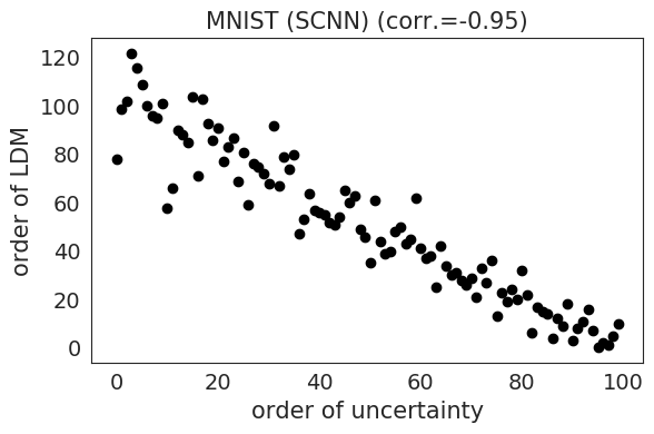
(a)

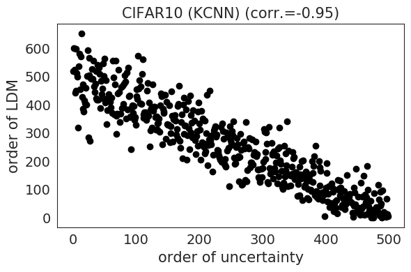
(b)

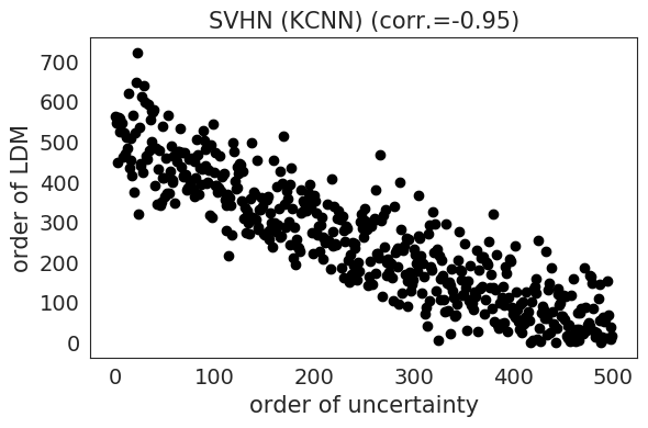
(c)

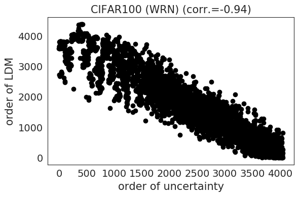
(d)

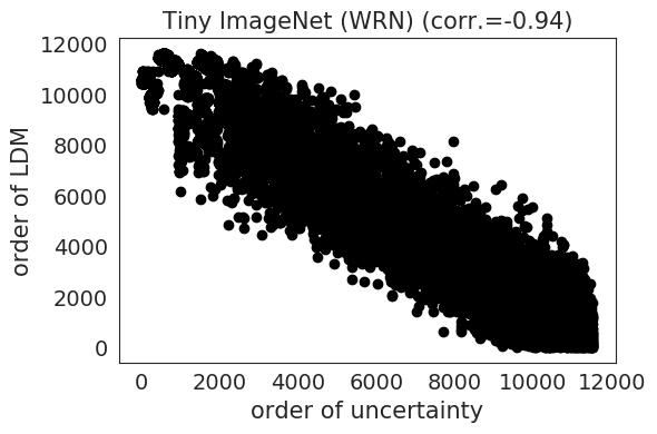
(e)

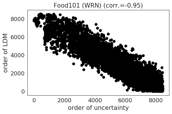
(f)

Figure 5: Examples of negative Spearman’s rank correlation between LDM order and uncertainty order on MNIST (a), CIFAR10 (b), SVHN (c), CIFAR100 (d), Tiny ImageNet (e), and FOOD101 (f).

Appendix C Theoretical Verifications of Intuitions for 2D Binary Classification with Linear Classifiers

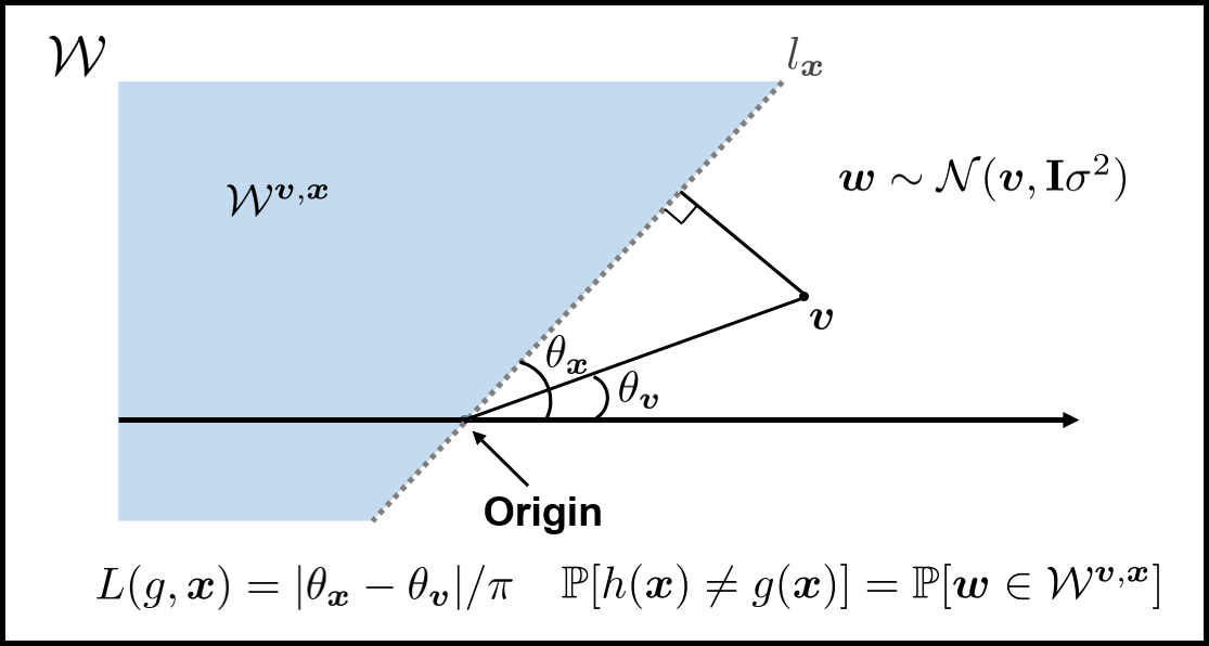
(a)

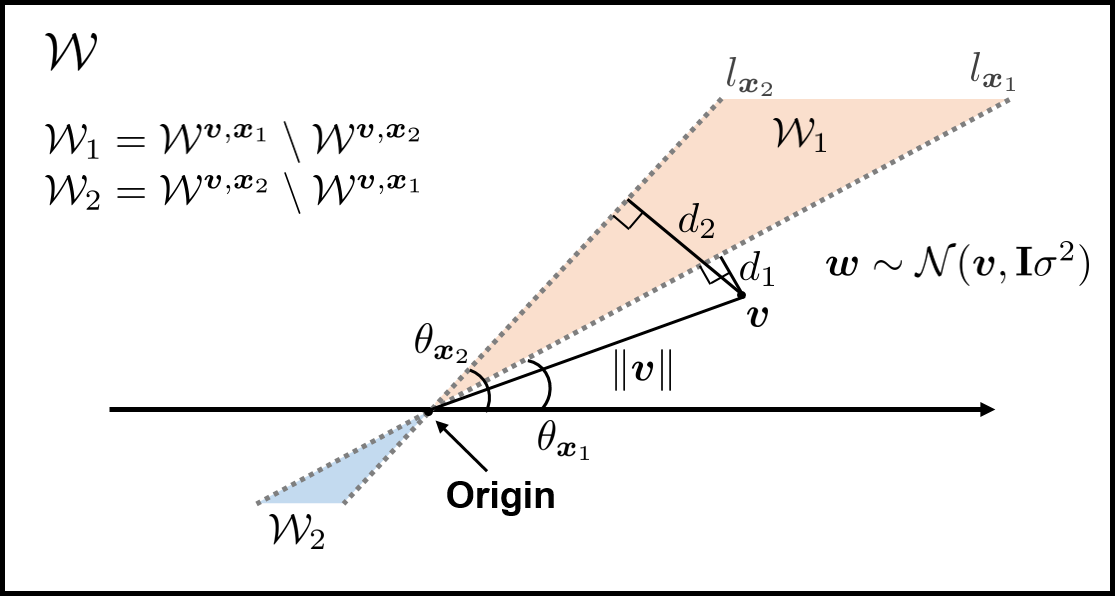
(b)

Figure 6: Proof of Proposition 1.

Here, we consider two-dimensional binary classification with a set of linear classifiers, $\mathcal{H}=\{h:h(\bm{x})=\operatorname*{sgn}(\bm{x}^{\mkern-1.5mu\mathsf{T}}\bm{w})\}$ where ${\bm{w}}\in\mathbb{R}^{2}$ is the parameter of $h$. We assume that $\bm{x}$ is uniformly distributed on $\mathcal{X}=\{\bm{x}:\|\bm{x}\|\leq 1\}\subset\mathbb{R}^{2}$. For a given $g\in{\mathcal{H}}$, let ${\bm{v}}$ be the parameter of $g$.

C.1 LDM as an Uncertainty Measure

Recall from Section 2.1 that the intuition behind a sample with a small LDM indicates that its prediction can be easily flip-flopped even by a small perturbation in the predictor. We theoretically prove this intuition

Proposition 1.

Suppose that $h$ is sampled with $\bm{w}\sim\mathcal{N}(\bm{v},\mathbf{I}\sigma^{2})$. Then,

$$L(g,\bm{x}_{1})<L(g,\bm{x}_{2})\Longleftrightarrow\mathbb{P}[h(\bm{x}_{1})\neq g(\bm{x}_{1})]>\mathbb{P}[h(\bm{x}_{2})\neq g(\bm{x}_{2})].$$

Figure 5 shows examples of Spearman’s rank correlation (Spearman, 1904) between the order of LDM and uncertainty, which is defined as the ratio of label predictions by a small perturbation in the predictor, on MNIST, CIFAR10, SVHN, CIFAR100, Tiny ImageNet, and FOOD101 datasets. Samples with increasing LDM or uncertainty are ranked from high to low. The results show that LDM order and uncertainty order have a strong negative rank correlation, and thus a sample with smaller LDM is closer to the decision boundary and is more uncertain.

Proof of Proposition 1.

One important observation is that by the duality between $\bm{w}$ and $\bm{x}$ (Tong & Chang, 2001), in $\mathbb{R}^{2}$, $\bm{w}$ is a point and $\bm{x}$ is represented by the hyperplane, $l_{\bm{x}}=\{\bm{w}\in\mathbb{R}^{2}:\operatorname*{sgn}(\bm{x}^{\mkern-1.5mu\mathsf{T}}\bm{w})=0\}$. Suppose that $h$ is sampled with $\bm{w}\sim\mathcal{N}(\bm{v},\mathbf{I}\sigma^{2})$, and let $\theta_{\bm{v}}$ be the angle of $\bm{v}$, $\theta_{\bm{x}}$ be the angle between $l_{\bm{x}}$ and positive x-axis, and $\mathcal{W}^{\bm{v},\bm{x}}$ be the half-plane divided by $l_{\bm{x}}$ which does not contain $\bm{v}$:

$$\mathcal{W}^{\bm{v},\bm{x}}=\{\bm{w}^{\prime}\in\mathcal{W}\mid h^{\prime}(\bm{x})\neq g(\bm{x})\}$$

as in Figure 6a. Then, $L(g,\bm{x})=|\theta_{\bm{x}}-\theta_{\bm{v}}|/\pi$ and $\mathbb{P}[h(\bm{x})\neq g(\bm{x})]=\mathbb{P}[\bm{w}\in\mathcal{W}^{\bm{v},\bm{x}}]$.

Let $d_{1},d_{2}$ be the distances between $\bm{v}$ and $l_{\bm{x}_{1}},l_{\bm{x}_{2}}$ respectively, and

$$\mathcal{W}_{1}=\mathcal{W}^{\bm{v},\bm{x}_{1}}\setminus\mathcal{W}^{\bm{v},\bm{x}_{2}},\quad\mathcal{W}_{2}=\mathcal{W}^{\bm{v},\bm{x}_{2}}\setminus\mathcal{W}^{\bm{v},\bm{x}_{1}}$$

as in Figure 6b. Suppose that $d_{1}<d_{2}$, then $|\theta_{\bm{x}_{1}}-\theta_{\bm{v}}|<|\theta_{\bm{x}_{2}}-\theta_{\bm{v}}|$ since $d_{i}=\|\bm{w}\|\sin|\theta_{\bm{x}_{i}}-\theta_{\bm{v}}|$, and

$$\mathbb{P}[\bm{w}\in\mathcal{W}^{\bm{v},\bm{x}_{1}}]-\mathbb{P}[\bm{w}\in\mathcal{W}^{\bm{v},\bm{x}_{2}}]=\mathbb{P}[\bm{w}\in\mathcal{W}_{1}]-\mathbb{P}[\bm{w}\in\mathcal{W}_{2}]>0$$

by the followings:

$$\mathcal{W}^{\bm{v},\bm{x}_{1}}=\mathcal{W}_{1}\cup(\mathcal{W}^{\bm{v},\bm{x}_{1}}\cap\mathcal{W}^{\bm{v},\bm{x}_{2}}),\quad\mathcal{W}^{\bm{v},\bm{x}_{2}}=\mathcal{W}_{2}\cup(\mathcal{W}^{\bm{v},\bm{x}_{1}}\cap\mathcal{W}^{\bm{v},\bm{x}_{2}})$$

where $\mathcal{W}_{1},\mathcal{W}_{2},$ and $\mathcal{W}^{\bm{v},\bm{x}_{1}}\cap\mathcal{W}^{\bm{v},\bm{x}_{2}}$ are disjoint. Note that $\mathcal{W}_{1}$ and $\mathcal{W}_{2}$ are one-to-one mapped by the symmetry at origin, but the probabilities are different by the biased location of ${\bm{v}}$, i.e, $\phi(\bm{w}_{1}|\bm{v},\sigma^{2})>\phi(\bm{w}_{2}|\bm{v},\sigma^{2})$ for all pairs of $(\bm{w}_{1},\bm{w}_{2})\in\mathcal{W}_{1}\times\mathcal{W}_{2}$ that are symmetric at the origin. Here $\phi(\cdot|\bm{v},\sigma^{2})$ is the probability density function of the bivariate normal distribution with mean $\bm{v}$ and covariance $\sigma^{2}\mathbf{I}$. Thus,

$$L(g,\bm{x}_{1})<L(g,\bm{x}_{2})\Longleftrightarrow d_{1}<d_{2}\Longleftrightarrow\mathbb{P}[h(\bm{x}_{1})\neq g(\bm{x}_{1})]>\mathbb{P}[h(\bm{x}_{2})\neq g(\bm{x}_{2})].$$

∎

C.2 Varying $\sigma^{2}$ in Algorithm 1

Recall from Section 2.2 that the intuition behind using multiple $\sigma^{2}$ is that it controls the trade-off between the probability of obtaining a hypothesis with a different prediction than that of $g$ and the scale of $\rho_{{}_{S}}(h,g)$. Theoretically, we show the following for two-dimensional binary classification with linear classifiers:

Proposition 2.

Suppose that $h$ is sampled with ${\bm{w}}\sim\mathcal{N}(\bm{v},\mathbf{I}\sigma^{2})$ where $\bm{w},\bm{v}\in\mathcal{W}$ are parameters of $h,g$ respectively, then $\mathbb{E}_{{\bm{w}}}[\rho(h,g)]$ is continuous and strictly increasing with $\sigma$.

Figure 7 shows the relationship between $\bar{\rho}_{{}_{S}}(h,g)$ and $\log\sigma$ for MNIST, CIFAR10, SVNH, CIFAR100, Tiny ImageNet, and FOOD101 datasets where $h$ is sampled with $\bm{w}\sim\mathcal{N}(\bm{v},\mathbf{I}\sigma^{2})$ and $\bar{\rho}_{{}_{S}}(h,g)$ is the mean of $\rho_{{}_{S}}(h,g)$ for sampled $h$s. The $\bar{\rho}_{{}_{S}}(h,g)$ is monotonically increasing with $\log\sigma$ in all experimental settings for general deep learning architectures.

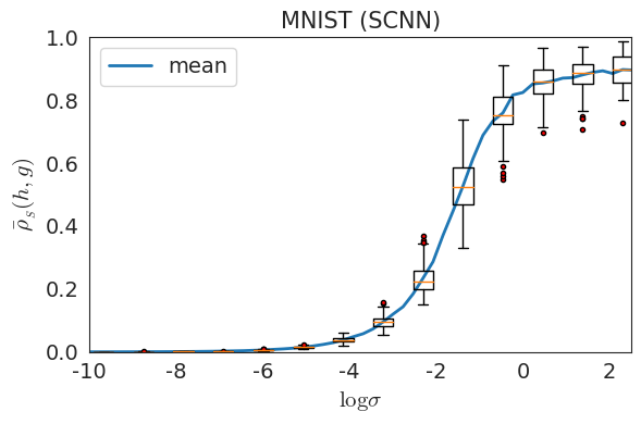
(a)

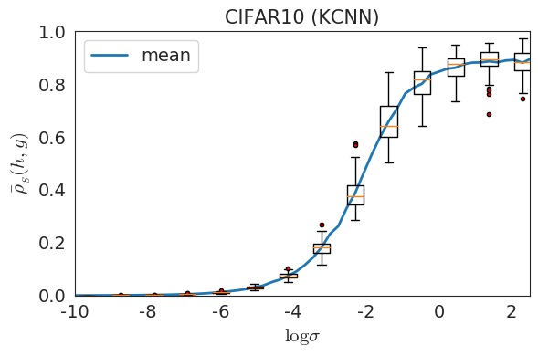
(b)

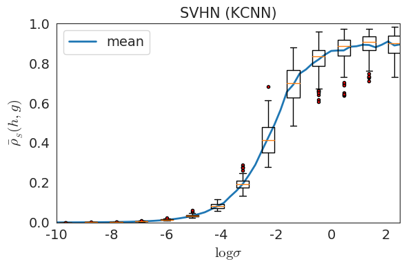
(c)

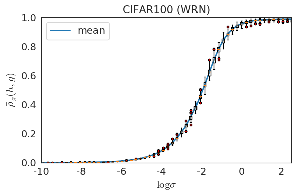
(d)

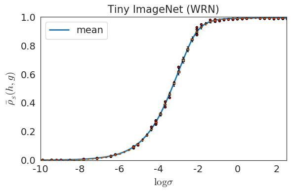
(e)

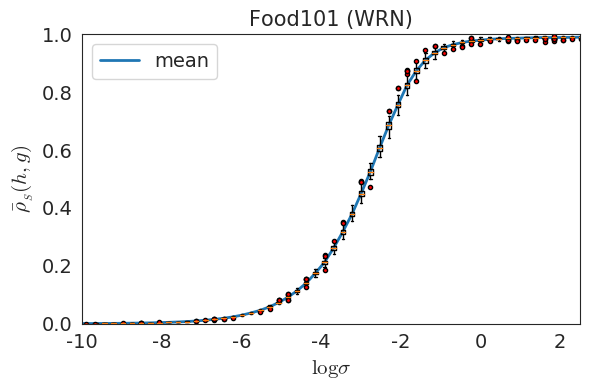
(f)

Figure 7: The relationship between the disagree metric and perturbation strength for MNIST (a), CIFAR10 (b), SVHN (c), CIFAR100 (d), Tiny ImageNet (e), and FOOD101 (f) datasets. $\bar{\rho}_{{}_{S}}(h,g)$ is monotonically increasing with the perturbation strength in all experimental settings.

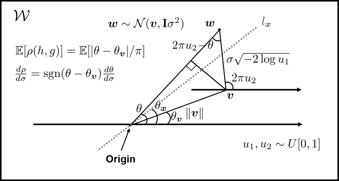
(a)

(b)

Figure 8: Proof of Proposition 2.

Proof of Proposition 2.

By the duality between $\bm{w}$ and $\bm{x}$, in $\mathcal{W}$, $\bm{w}$ is a point and $\bm{x}$ is represented by the hyperplane, $l_{\bm{x}}=\{\bm{w}\in\mathcal{W}:\operatorname*{sgn}(\bm{x}^{\mkern-1.5mu\mathsf{T}}\bm{w})=0\}$. Let $h$ be a sampled hypothesis with $\bm{w}\sim\mathcal{N}(\bm{v},\mathbf{I}\sigma^{2})$, $\theta_{\bm{v}}$ be the angle of $\bm{v}=(v_{1},v_{2})^{\mkern-1.5mu\mathsf{T}}$, i.e., $\tan\theta_{\bm{v}}=v_{2}/v_{1}$, $\theta$ be the angle of $\bm{w}=(w_{1},w_{2})^{\mkern-1.5mu\mathsf{T}}$, i.e., $\tan\theta=w_{2}/w_{1}$, and $\theta_{\bm{x}}$ be the angle between $l_{\bm{x}}$ and positive x-axis. Here, $\theta,\theta_{\bm{x}}\in[-\pi+\theta_{\bm{v}},\pi+\theta_{\bm{v}}]$ in convenience. When $\theta_{\bm{x}}$ or $\pi+\theta_{\bm{x}}$ is between $\theta$ and $\theta_{\bm{v}}$, $h(\bm{x})\neq g(\bm{x})$, otherwise $h(\bm{x})=g(\bm{x})$. Thus, $\rho(h,g)=|\theta-\theta_{\bm{v}}|/\pi$.

Using Box-Muller transform (Box & Muller, 1958), $\bm{w}$ can be generated by

$$w_{1}=v_{1}+\sigma\sqrt{-2\log u_{1}}\cos(2\pi u_{2}),\ w_{2}=v_{2}+\sigma\sqrt{-2\log u_{1}}\sin(2\pi u_{2})$$

where $u_{1}$ and $u_{2}$ are independent uniform random variables on $[0,1]$. Then, $\|\bm{w}-\bm{v}\|=\sigma\sqrt{-2\log u_{1}}$ and $(w_{2}-v_{2})/(w_{1}-v_{1})=\tan(2\pi u_{2})$, i.e., the angle of $\bm{w}-\bm{v}$ is $2\pi u_{2}$. Here,

$$\|\bm{v}\|\sin(\theta-\theta_{\bm{v}})=\sigma\sqrt{-2\log u_{1}}\sin(2\pi u_{2}-\theta)$$ (8)

by using the perpendicular line from $\bm{v}$ to the line passing through the origin and $\bm{w}$ (see the Figure 8 for its geometry), and Eq. 8 is satisfied for all $\theta$. For given $u_{1}$ and $u_{2}$, $\theta$ is continuous and the derivative of $\theta$ with respect to $\sigma$ is

$$\frac{d\theta}{d\sigma}=\frac{\sqrt{-2\log u_{1}}\sin^{2}(2\pi u_{2}-\theta)}{\|\bm{v}\|\sin(2\pi u_{2}-\theta_{\bm{v}})},\quad\text{thus}\quad\left\{\begin{array}[]{cc}\frac{d\theta}{d\sigma}>0,&u_{2}\in(\frac{\theta_{\bm{v}}}{2\pi},\frac{\pi+\theta_{\bm{v}}}{2\pi})\\ \frac{d\theta}{d\sigma}<0,&u_{2}\in[0,1]\setminus[\frac{\theta_{\bm{v}}}{2\pi},\frac{\pi+\theta_{\bm{v}}}{2\pi}]\end{array}\right..$$

Then,

$$\frac{d\rho(h,g)}{d\sigma}=\operatorname*{sgn}(\theta-\theta_{\bm{v}})\frac{d\theta}{d\sigma}>0\quad\text{where}\quad u_{2}\notin\Big{\{}\frac{\theta_{\bm{v}}}{2\pi},\frac{\pi+\theta_{\bm{v}}}{2\pi}\Big{\}}.$$

Thus, $\rho(h,g)$ is continuous and strictly increasing with $\sigma$ when $u_{2}\neq\frac{\theta_{\bm{v}}}{2\pi}$ and $u_{2}\neq\frac{\pi+\theta_{\bm{v}}}{2\pi}$. Let $\rho(h,g)=F(\sigma,u_{1},u_{2})$, then $\mathbb{E}_{{\bm{w}}}[\rho(h,g)]=\int F(\sigma,u_{1},u_{2})f(u_{1})f(u_{2})du_{1}du_{2}$ where $f(u_{i})=\mathbb{I}[0<u_{i}<1]$. For $0<\sigma_{1}<\sigma_{2}$,

$$\mathbb{E}_{{\bm{w}}\sim{\mathcal{N}}({\bm{v}},\mathbf{I}\sigma_{2}^{2})}[\rho(h,g)]-\mathbb{E}_{{\bm{w}}\sim{\mathcal{N}}({\bm{v}},\mathbf{I}\sigma_{1}^{2})}[\rho(h,g)]$$

$$=\int\left(F(\sigma_{2},u_{1},u_{2})-F(\sigma_{1},u_{1},u_{2})\right)f(u_{1})f(u_{2})du_{1}du_{2}>0.$$

∎

C.3 Assumption 3 Holds with Gaussian Sampling

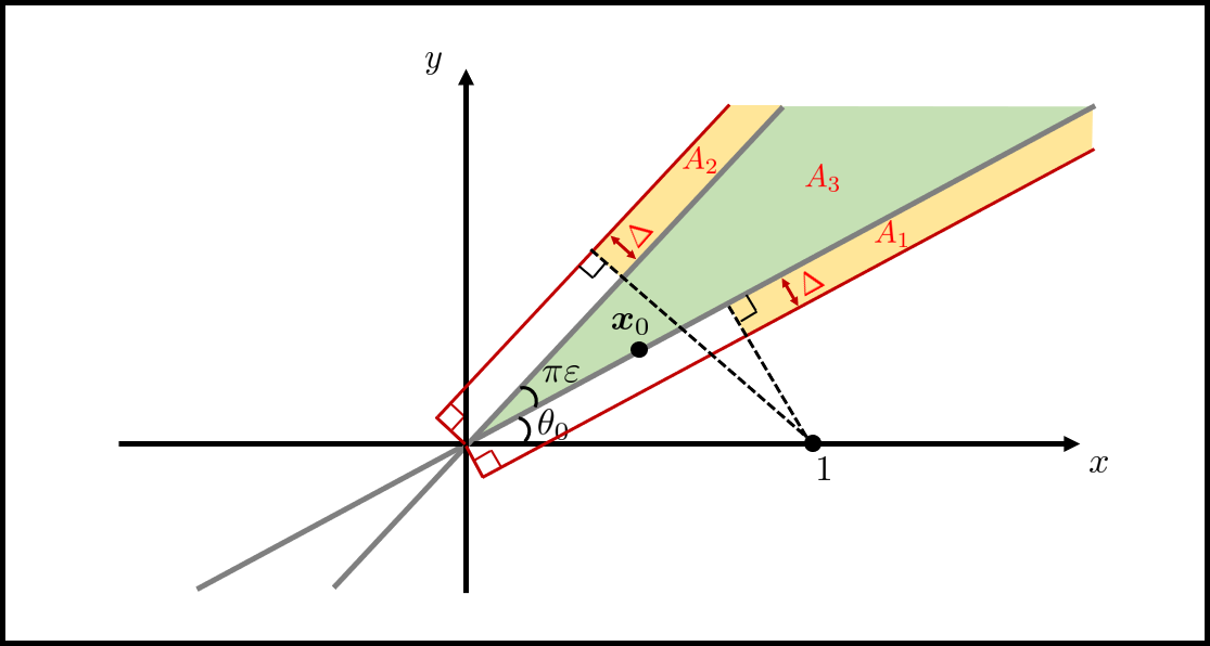
(a)

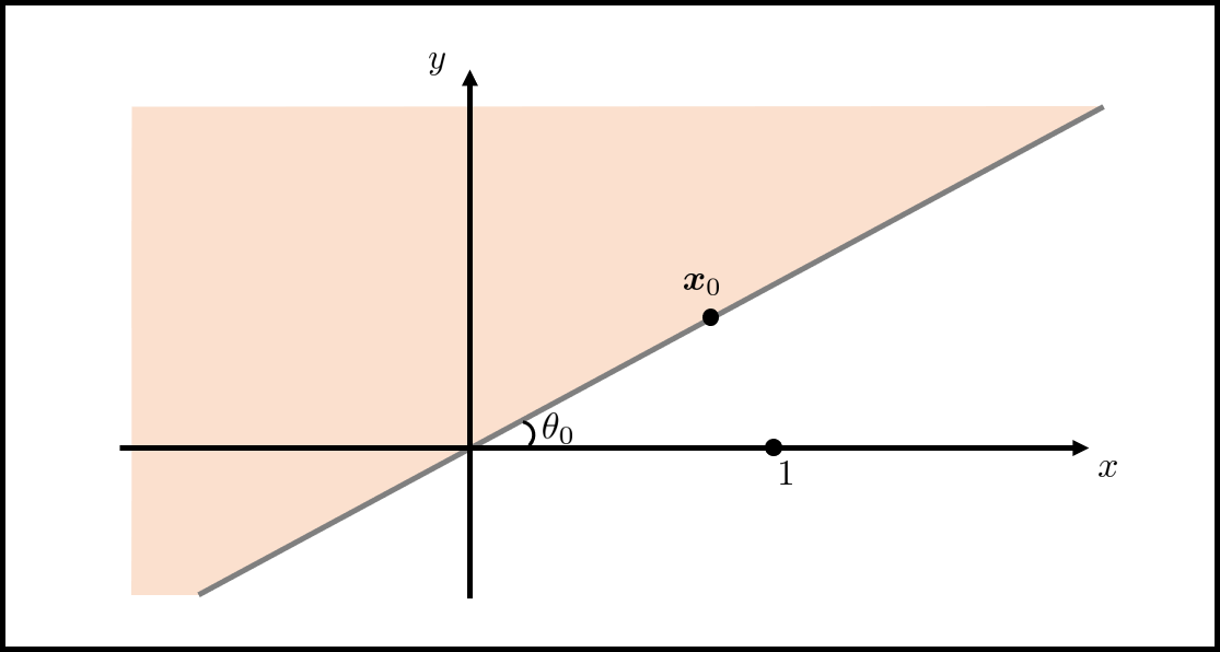
(b)

Figure 9: Proof of Proposition 3.

Proposition 3.

Assume that the given sample ${\bm{x}}_{0}$ forms an angle $\theta_{0}\in(0,\pi/2)$ w.r.t. the x-axis, and consider $\varepsilon\in(0,1)$ such that $\theta_{0}+\pi\varepsilon<\frac{\pi}{2}$. Then, for binary classification with linear hypotheses and ${\mathcal{H}}_{N}$ comprising of $N$ i.i.d. random samples from ${\mathcal{N}}((1,0),\sigma^{2}{\bm{I}}_{2})$ for some fixed $\sigma^{2}>0$, Assumption 3 holds with $\alpha(N,\varepsilon)={\mathcal{O}}\left(\frac{1}{\sqrt{N}}\right)$ and $\beta(N)={\mathcal{O}}\left(e^{-\sqrt{N}}\right)$.

Proof.

We want to show that there exists $\alpha(N,\cdot)$ and $\beta(N)$ with $\lim_{N\rightarrow\infty}\alpha(N,\cdot)=\lim_{N\rightarrow\infty}\beta(N)=0$ such that

$${\mathbb{P}}\left[\inf_{{\bm{w}}^{*}:\theta({\bm{w}}^{*})\in(\theta_{0},\theta_{0}+\pi\varepsilon)}\min_{{\bm{w}}\in{\mathcal{H}}_{N}^{g,{\bm{x}}_{0}}}\lVert{\bm{w}}^{*}-{\bm{w}}\rVert_{2}\geq\frac{1}{B}\alpha(N,\varepsilon)\right]\leq\beta(N),$$

where $\theta({\bm{w}}^{*})$ is the angle made between ${\bm{w}}^{*}$ and the x-axis. Note that ${\mathcal{H}}_{N}^{g,{\bm{x}}_{0}}$ is random as well. Thus, we make use of a peeling argument as follows: conditioned on the event that $|{\mathcal{H}}_{N}^{g,{\bm{x}}_{0}}|=S$ for $S\in[N]$, we have that for any $\Delta\in(0,\sin\theta_{0})$,

$${\mathbb{P}}\left[\inf_{{\bm{w}}^{*}:\theta(h_{{\bm{w}}^{*}})\in(\theta_{0},\theta_{0}+\pi\varepsilon)}\min_{{\bm{w}}\in{\mathcal{H}}_{N}^{g,{\bm{x}}_{0}}}\lVert{\bm{w}}^{*}-{\bm{w}}\rVert_{2}\geq\Delta\ \Bigg{|}\ |{\mathcal{H}}_{N}^{g,{\bm{x}}_{0}}|=S\right]=\left(1-p(\theta_{0},\Delta,\varepsilon)\right)^{S},$$

where $p(\theta_{0},\Delta,\varepsilon)$ is the measure of the region enclosed by the red boundary in Fig. 9a w.r.t. ${\mathcal{N}}((1,0),\sigma^{2}{\bm{I}}_{2})$. Also, we have that for $S\in[N]$

$${\mathbb{P}}\left[|{\mathcal{H}}_{N}^{g,{\bm{x}}_{0}}|=S\right]=\binom{N}{S}q(\theta_{0})^{S}(1-q(\theta_{0}))^{N-S},$$

where $q(\theta_{0})$ is the measure of the (light) red region in Fig. 9b w.r.t. ${\mathcal{N}}((1,0),\sigma^{2}{\bm{I}}_{2})$.

Thus, we have that

$${\mathbb{P}}\left[\inf_{{\bm{w}}^{*}:\theta({\bm{w}}^{*})\in(\theta_{0},\theta_{0}+\pi\varepsilon)}\min_{{\bm{w}}\in{\mathcal{H}}_{N}^{g,{\bm{x}}_{0}}}\lVert{\bm{w}}^{*}-{\bm{w}}\rVert_{2}\geq\Delta\right]$$

$$=\sum_{S=0}^{N}{\mathbb{P}}\left[\inf_{{\bm{w}}^{*}:\theta({\bm{w}}^{*})\in(\theta_{0},\theta_{0}+\pi\varepsilon)}\min_{{\bm{w}}\in{\mathcal{H}}_{N}^{g,{\bm{x}}_{0}}}\lVert{\bm{w}}^{*}-{\bm{w}}\rVert_{2}\geq\Delta\ \Bigg{|}\ |{\mathcal{H}}_{N}^{g,{\bm{x}}_{0}}|=S\right]{\mathbb{P}}\left[|{\mathcal{H}}_{N}^{g,{\bm{x}}_{0}}|=S\right]$$

$$=\sum_{S=0}^{N}\binom{N}{S}q(\theta_{0})^{S}(1-q(\theta_{0}))^{N-S}\left(1-p(\theta_{0},\Delta,\varepsilon)\right)^{S}$$

$$=\left((1-q(\theta_{0}))+q(\theta_{0})(1-p(\theta_{0},\Delta,\varepsilon))\right)^{N}$$

$$=\left(1-p(\theta_{0},\Delta,\varepsilon)q(\theta_{0})\right)^{N}$$

$$\leq e^{-Np(\theta_{0},\Delta,\varepsilon)q(\theta_{0})},$$

where the last inequality follows from the simple fact that $1+x\leq e^{x}$ for any $x\in{\mathbb{R}}$.

Now it suffices to obtain non-vacuous lower bounds of $p(\theta_{0},\Delta,\varepsilon)$ and $q(\theta_{0})$.

Lower bounding $q(\theta_{0})$.

By rotational symmetry of ${\mathcal{N}}((1,0),\sigma^{2}{\bm{I}}_{2})$ and the fact that rotation preserves Euclidean geometry, this is equivalent to finding the probability measure of the lower half-plane under the Gaussian distribution ${\mathcal{N}}((0,\sin\theta_{0}),\sigma^{2}{\bm{I}}_{2})$, which is as follows:

$$q(\theta_{0}) =\frac{1}{2\pi\sigma^{2}}\int_{-\infty}^{0}\int_{-\infty}^{\infty}\exp\left(-\frac{x^{2}+(y-\sin\theta_{0})^{2}}{2\sigma^{2}}\right)dxdy$$

$$=\frac{1}{\sqrt{2\pi}\sigma}\int_{-\infty}^{-\sin\theta_{0}}\exp\left(-\frac{y^{2}}{2\sigma^{2}}\right)dy$$

$$=\frac{1}{2}-\frac{1}{\sqrt{2\pi}\sigma}\int_{0}^{\sin\theta_{0}}\exp\left(-\frac{y^{2}}{2\sigma^{2}}\right)dy$$

$$\overset{(*)}{\geq}\frac{1}{2}-\frac{1}{\sqrt{2\pi}\sigma}\int_{0}^{\sin\theta_{0}}\left(\frac{2\sigma^{2}}{(\sin\theta_{0})^{2}}\left(1-\exp\left(-\frac{(\sin\theta_{0})^{2}}{2\sigma^{2}}\right)\right)y+1\right)dy$$

$$=\frac{1}{2}-\frac{1}{\sqrt{2\pi}\sigma}\left(\sigma^{2}\left(1-\exp\left(-\frac{(\sin\theta_{0})^{2}}{2\sigma^{2}}\right)\right)+\sin\theta_{0}\right)$$

$$=\frac{1}{2}-\frac{1}{\sqrt{2\pi}}\left(\sigma\left(1-\exp\left(-\frac{(\sin\theta_{0})^{2}}{2\sigma^{2}}\right)\right)+\frac{\sin\theta_{0}}{\sigma}\right),$$

where $(*)$ follows from the simple observation that $e^{x}\leq\frac{1-e^{-a}}{a}x+1$ for $x\in[-a,0]$ and $a>0$.

Lower bounding $p(\theta_{0},\Delta,\varepsilon)$.

Via similar rotational symmetry arguments and geometric decomposition of the region enclosed by the red boundary (see Fig. 9a), we have that

$$p(\theta_{0},\Delta,\varepsilon)$$

$$\geq A_{1}+A_{2}+A_{3}$$ (see Fig. 9a)

$$\geq\frac{1}{2\pi\sigma^{2}}\int_{0}^{\Delta}\int_{0}^{\infty}\exp\left(-\frac{x^{2}+(y-\sin\theta_{0})^{2}}{2\sigma^{2}}\right)dxdy$$

$$\quad+\frac{1}{2\pi\sigma^{2}}\int_{-\Delta}^{0}\int_{0}^{\infty}\exp\left(-\frac{x^{2}+(y-\sin(\theta_{0}+\pi\varepsilon))^{2}}{2\sigma^{2}}\right)dxdy$$

$$\quad+\frac{1}{2\pi\sigma^{2}}\int_{\theta_{0}}^{\theta_{0}+\pi\varepsilon}\int_{0}^{\infty}\exp\left(-\frac{(r\cos\theta-1)^{2}+(r\sin\theta)^{2}}{2\sigma^{2}}\right)rdrd\theta$$

$$=\frac{1}{2\sqrt{2\pi}\sigma}\int_{-\sin\theta_{0}}^{\Delta-\sin\theta_{0}}\exp\left(-\frac{y^{2}}{2\sigma^{2}}\right)dy+\frac{1}{2\sqrt{2\pi}\sigma}\int_{\sin(\theta_{0}+\pi\varepsilon)}^{\Delta+\sin(\theta_{0}+\pi\varepsilon)}\exp\left(-\frac{y^{2}}{2\sigma^{2}}\right)dy$$

$$\quad+\frac{1}{2\pi\sigma^{2}}\int_{\theta_{0}}^{\theta_{0}+\pi\varepsilon}\int_{0}^{\infty}\exp\left(-\frac{r^{2}-2r\cos\theta+1}{2\sigma^{2}}\right)rdrd\theta$$

$$\geq\frac{\Delta}{2\sqrt{2\pi}\sigma}\exp\left(-\frac{(\sin\theta_{0})^{2}}{2\sigma^{2}}\right)+\frac{\Delta}{2\sqrt{2\pi}\sigma}\exp\left(-\frac{(\Delta+\sin(\theta_{0}+\pi\varepsilon))^{2}}{2\sigma^{2}}\right)$$

$$\quad+\frac{\varepsilon}{2\sigma^{2}}\int_{0}^{\infty}r\exp\left(-\frac{r^{2}+1}{2\sigma^{2}}\right)dr$$

$$\geq\frac{\Delta}{\sqrt{2\pi}\sigma}\exp\left(-\frac{(\sin\theta_{0}+1)^{2}}{2\sigma^{2}}\right)+\frac{\varepsilon}{2}\exp\left(-\frac{1}{2\sigma^{2}}\right).$$

By choosing $\Delta={\mathcal{O}}\left(\frac{1}{\sqrt{N}}\right)$, the proposition holds. ∎

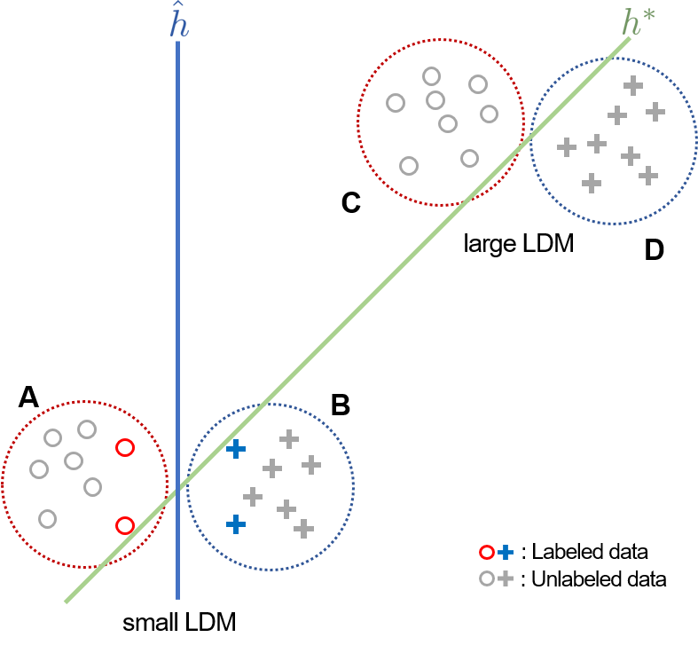
Figure 10: The effect of LDM-based seeding. Considering only LDM, samples are selected only in A or B, but samples in C or D are also selected if the seeding method is applied.

C.4 Effect of Diversity in LDM-S

Here, we provide more intuition on why samples selected in the order of the smallest empirical LDM may not be the best strategy, and thus why need to pursue diversity via seeding, which was verified in realistic scenarios in Section 4.2. Again, let us consider a realizable binary classification with a set of linear classifiers, i.e., there exists $h^{*}$ whose test error is zero (See Figure 10). Let the red circles and blue crosses be the labeled samples and $g$ be the given hypotheses learned by the labeled samples. In this case, samples’ LDM in groups A or B are small, and those in groups C or D are large. Thus, the algorithm will always choose samples in groups A or B if we do not impose diversity and choose only samples with the smallest LDM. However, the samples in groups C or D are the samples that are more helpful to us in this case, i.e., provide more information. Therefore, pursuing diversity is necessary to provide the chance to query samples in C and D.

Appendix D Datasets, Networks and Experimental Settings

D.1 Datasets

OpenML#6 (Frey & Slate, 1991) is a letter image recognition dataset which has $20,000$ samples in $26$ classes. Each sample has $16$ numeric features. In experiments, it is split into two parts: $16,000$ samples for training and $4,000$ samples for test.

OpenML#156 (Vanschoren et al., 2014) is a synthesized dataset for random RBF which has $100,000$ samples in $5$ classes. Each sample has $10$ numeric features. In experiments, a subset is split into two parts: $40,000$ samples for training and $10,000$ samples for test.

OpenML#44135 (Fanty & Cole, 1990) is a isolated letter speech recognition dataset which has $7,797$ samples in $26$ classes. Each sample has $614$ numeric features. In experiments, it is split into two parts: $6,237$ samples for training and $1,560$ samples for test.

MNIST (Lecun et al., 1998) is a handwritten digit dataset which has $60,000$ training samples and $10,000$ test samples in $10$ classes. Each sample is a black and white image and $28\times 28$ in size.

CIFAR10 and CIFAR100 (Krizhevsky, 2009) are tiny image datasets which has $50,000$ training samples and $10,000$ test samples in $10$ and $100$ classes respectively. Each sample is a color image and $32\times 32$ in size.

SVHN (Netzer et al., 2011) is a real-world digit dataset which has $73,257$ training samples and $26,032$ test samples in $10$ classes. Each sample is a color image and $32\times 32$ in size.

Tiny ImageNet (Le & Yang, 2015) is a subset of the ILSVRC (Russakovsky et al., 2015) dataset which has $100,000$ samples in $200$ classes. Each sample is a color image and $64\times 64$ in size. In experiments, Tiny ImageNet is split into two parts: $90,000$ samples for training and $10,000$ samples for test.

FOOD101 (Bossard et al., 2014) is a fine-grained food image dataset which has $75,750$ training samples and $25,250$ test samples in $101$ classes. Each sample is a color image and resized to $75\times 75$.

ImageNet (Russakovsky et al., 2015) is an image dataset organized according to the WordNet hierarchy which has $1,281,167$ training samples and $50,000$ validation samples (we use the validation samples as test samples) in $1,000$ classes.

Table 3: Settings for data and acquisition size. Acquisition size denotes the number of initial labeled samples + query size for each step (the size of pool data) $\rightarrow$ the number of final labeled samples.

Dataset	Model	# of parameters sampled / total	Data size train / validation / test	Acquisition size
OpenML#6	MLP	3.4K/22.0K	16,000 / - / 4,000	200	+200 (2K)	$\rightarrow$ 4,000
OpenML#156	MLP	0.6K/18.6K	40,000 / - / 10,000	100	+100 (2K)	$\rightarrow$ 2,000
OpenML#44135	MLP	3.4K/98.5K	6,237 / - / 1,560	100	+100 (2K)	$\rightarrow$ 2,000
MNIST	S-CNN	1.3K/1.2M	55,000 / 5,000 / 10,000	20	+20 (2,000)	$\rightarrow$ 1,020
CIFAR10	K-CNN	5.1K/2.2M	45,000 / 5,000 / 10,000	200	+400 (4,000)	$\rightarrow$ 9,800
SVHN	K-CNN	5.1K/2.2M	68,257 / 5,000 / 26,032	200	+400 (4,000)	$\rightarrow$ 9,800
CIFAR100	WRN-16-8	51.3K/11.0M	45,000 / 5,000 / 10,000	5,000	+2,000 (10,000)	$\rightarrow$ 25,000
Tiny ImageNet	WRN-16-8	409.8K/11.4M	90,000 / 10,000 / 10,000	10,000	+5,000 (20,000)	$\rightarrow$ 50,000
FOOD101	WRN-16-8	206.9K/11.2M	60,600 / 15,150 / 25,250	6,000	+3,000 (15,000)	$\rightarrow$ 30,000
ImageNet	ResNet-18	513K/11.7M	1,153,047 / 128,120 / 50,000	128,120	+64,060 (256,240)	$\rightarrow$ 384,360

Table 4: Settings for training.

Dataset	Model	Epochs	Batch size	Optimizer	Learning Rate	Learning Rate Schedule $\times$decay [epoch schedule]
OpenML#6	MLP	100	64	Adam	0.001	-
OpenML#156	MLP	100	64	Adam	0.001	-
OpenML#44135	MLP	100	64	Adam	0.001	-
MNIST	S-CNN	50	32	Adam	0.001	-
CIFAR10	K-CNN	150	64	RMSProp	0.0001	-
SVHN	K-CNN	150	64	RMSProp	0.0001	-
CIFAR100	WRN-16-8	100	128	Nesterov	0.05	$\times$0.2 [60, 80]
Tiny ImageNet	WRN-16-8	200	128	Nesterov	0.1	$\times$0.2 [60, 120, 160]
FOOD101	WRN-16-8	200	128	Nesterov	0.1	$\times$0.2 [60, 120, 160]
ImageNet	ResNet-18	100	128	Nesterov	0.001	$\times$0.2 [60, 80]

D.2 Deep Networks

MLP consists of [128 dense - dropout ($0.3$) - 128 dense - dropout ($0.3$) - # class dense - softmax] layers, and it is used for OpenML datasets.

S-CNN (Chollet et al., 2015) consists of [3$\times$3$\times$32 conv $-$ 3$\times$3$\times$ 64 conv $-$ 2$\times$2 maxpool $-$ dropout ($0.25$) $-$ $128$ dense $-$ dropout ($0.5$) $-$ # class dense $-$ softmax] layers, and it is used for MNIST.

K-CNN (Chollet et al., 2015) consists of [two 3$\times$3$\times$32 conv $-$ 2$\times$2 maxpool - dropout ($0.25$) $-$ two 3$\times$3$\times$64 conv $-$ 2$\times$2 maxpool - dropout ($0.25$) $-$ $512$ dense $-$ dropout ($0.5$) $-$ # class dense - softmax] layers, and it is used for CIFAR10 and SVHN.

WRN-16-8 (Zagoruyko & Komodakis, 2016) is a wide residual network that has 16 convolutional layers and a widening factor 8, and it is used for CIFAR100, Tiny ImageNet, and FOOD101.

ResNet-18 (He et al., 2016) is a residual network that is a 72-layer architecture with 18 deep layers, and it is used for ImageNet.

D.3 Experimental Settings

The experimental settings for active learning regarding dataset, architecture, number of parameters, data size, and acquisition size are summarized in Table 3. Training settings regarding a number of epochs, batch size, optimizer, learning rate, and learning rate schedule are summarized in Table 4. The model parameters are initialized with He normal initialization (He et al., 2015) for all experimental settings. For all experiments, the initial labeled samples for each repetition are randomly sampled according to the distribution of the training set.

Appendix E Performance Profile and Penalty Matrix

E.1 Performance Profile

The performance profile, known as the Dolan-Moré plot, has been widely considered in benchmarking active learning (Tsymbalov et al., 2018; 2019), optimization profiles (Dolan & Moré, 2002), and even general deep learning tasks (Burnaev et al., 2015a; b). To introduce the Dolan-Moré plot, let $\mathrm{acc}_{A}^{D,r,t}$ be the test accuracy of algorithm $A$ at step $t\in[T_{D}]$, for dataset $D$ and repetition $r\in[R]$, and $\Delta_{A}^{D,r,t}=\max_{A^{\prime}}(\mathrm{acc}_{A^{\prime}}^{D,r,t})-\mathrm{acc}_{A}^{D,r,t}$. Here, $T_{D}$ is the number of steps for dataset $D$, and $R$ is the total number of repetitions. Then, we define the performance profile as

$$R_{A}(\delta):=\frac{1}{n_{{}_{D}}}\sum_{D}\left[\frac{\sum_{r,t}\mathbb{I}(\Delta_{A}^{D,r,t}\leq\delta\ )}{RT_{D}}\right],$$

where $n_{{}_{D}}$ is the number of datasets. Intuitively, $R_{A}(\delta)$ is the fraction of cases where the performance gap between algorithm $A$ and the best competitor is less than $\delta$. Specifically, when $\delta=0$, $R_{A}(0)$ is the fraction of cases on which algorithm $A$ performs the best.

E.2 Penalty Matrix

The penalty matrix $P=(P_{ij})$ is evaluated as done in Ash et al. (2020): For each dataset, step, and each pair of algorithms ($A_{i}$, $A_{j}$), we have 5 test accuracies $\{\mathrm{acc}_{i}^{r}\}_{r=1}^{5}$ and $\{\mathrm{acc}_{j}^{r}\}_{r=1}^{5}$ respectively. We compute the $t$-score as $t=\sqrt{5}\bar{\mu}/\bar{\sigma}$, where $\bar{\mu}=\frac{1}{5}\sum_{r=1}^{5}(\mathrm{acc}_{i}^{r}-\mathrm{acc}_{j}^{r})$ and $\bar{\sigma}=\sqrt{\frac{1}{4}\sum_{r=1}^{5}(\mathrm{acc}_{i}^{r}-\mathrm{acc}_{j}^{r}-\bar{\mu})^{2}}$. The two-sided paired sample $t$-test is performed for the null that there is no performance difference between algorithms: $A_{i}$ is said to beat $A_{j}$ when $t>2.776$ (the critical point of $p$-value being $0.05$), and vice-versa when $t<-2.776$. Then when $A_{i}$ beats $A_{j}$, we accumulate a penalty of $1/T_{D}$ to $P_{i,j}$ where $T_{D}$ is the number of steps for dataset $D$, and vice-versa. Summing across the datasets gives us the final penalty matrix.

Appendix F Ablation Study

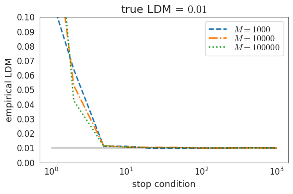
(a)

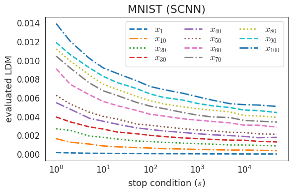
(b)

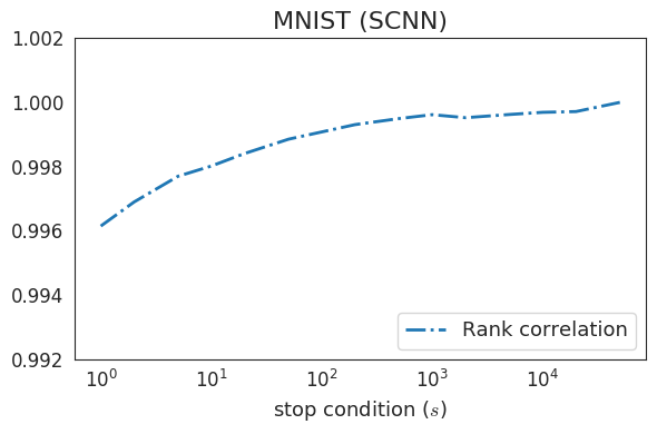
(c)

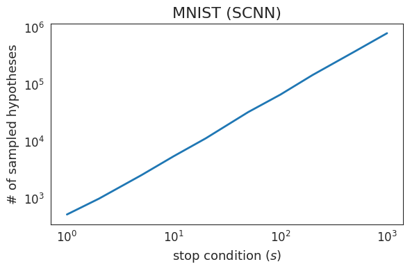
(d)

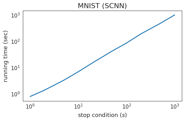
(e)

Figure 11: Empirically evaluated LDMs by Algorithm 1 with respect to the stop condition $s$. (a) Here, we consider the two-dimensional binary classification with the linear classifier (see Figure 1). The evaluated LDM is close to the true LDM even when $s=10$ and reaches the true LDM when $s\geq 20$. (b) Evaluated LDMs of MNIST samples with a four-layered CNN. Observe that the evaluated LDM monotonically decreases as $s$ increases, and the rank order is well maintained. (c) In the same setting, the rank correlation coefficient of the evaluated LDMs of a range of $s$’s to that at $s=50000$. Note that already at $s=10$, the rank correlation coefficient is $0.998$, suggesting that $s=10$ suffices. (d-e) The number of sampled hypotheses and runtime for evaluating LDM are almost linearly proportional to the stop condition.

F.1 Choice of Stop Condition $s$

Figure 11a shows the empirically evaluated LDM by Algorithm 1 in binary classification with the linear classifier as described in Figure 1. In the experiment, the true LDM of the sample is set to $0.01$. The evaluated LDM is very close to the true LDM when $s=10$ and reaches the true LDM when $s\geq 20$ with the gap being roughly $10^{-4}$. This suggests that even with a moderate value of $s$, Algorithm 1 can approximate the true LDM with sufficiently low error.

Figure 11b shows the empirically evaluated LDMs of MNIST samples for a four-layered CNN where $M$ is set to be the total number of samples in MNIST, which is $60000$. We denote ${\bm{x}}_{i}$ as the $i\textsuperscript{th}$ sample ordered by the final evaluated LDM. Observe that the evaluated LDMs are monotonically decreasing as $s$ increases, and they seem to converge while maintaining the rank order. In practice, a large $s$ for obtaining values close to the true LDM is computationally prohibitive as the algorithm requires huge runtime to sample a large number of hypotheses. For example, when $s=50000$, our algorithm samples $\sim$50M hypotheses and takes roughly 18 hours to run and evaluate LDM. Therefore, based upon the observation that the rank order is preserved throughout the values of $s$, we focus on the rank order of the evaluated LDMs rather than their true values.

Figure 11c shows the rank correlation coefficient of the evaluated LDMs of a range of $s$’s to that at $s=50000$. Even when $s=10$, the rank correlation coefficient between $s=10$ and $s=50000$ is already $0.998$. We observed that the same properties of the evaluated LDMs w.r.t. the stop condition $s$ also hold for other datasets, i.e., the preservation of rank order holds in general.

Figure 11d and 11e show the number of sampled hypotheses and runtime with respect to the stop condition when LDM is evaluated. Both are almost linearly proportional to the stop condition and thus we should set the stop condition as small as possible to reduce the running time in LDM evaluation.

F.2 Effectiveness of LDM

To isolate the effectiveness of LDM, we consider three other variants of LDM-S. ‘LDM-smallest’ select batches with the smallest LDMs without taking diversity into account, ‘Seeding (cos)’ and ‘Seeding ($\ell_{2}$)’ are the unweighted $k$-means++ seeding methods using cosine and $\ell_{2}$ distance, respectively. Note that the last two do not use LDM in any way. We have excluded batch diversity to further clarify the effectiveness of LDM.

Figure 12 shows the test accuracy with respect to the number of labeled samples on MNIST, CIFAR10, and CIFAR100 datasets. Indeed, we observe a significant performance improvement when using LDM and a further improvement when batch diversity is considered. Additional experiments are conducted to compare the $k$-means++ seeding with FASS (Wei et al., 2015) or Cluster-Margin (Citovsky et al., 2021), which can be a batch diversity method for LDM. Although FASS helps LDM slightly, it falls short of LDM-S. Cluster-Margin also does not help LDM and, surprisingly, degrades the performance. We believe this is because Cluster-Margin strongly pursues batch diversity, diminishing the effect of LDM as an uncertainty measure. Specifically, Cluster-Margin considers samples of varying LDM scores from the beginning (a somewhat large portion of them are thus not so useful). In contrast, our algorithm significantly weights the samples with small LDM, biasing our samples towards more uncertain samples (and thus more useful).

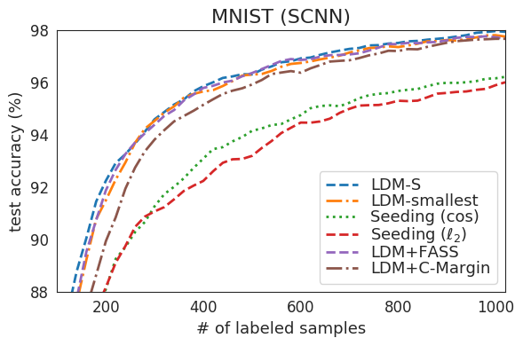
(a)

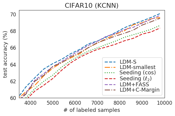
(b)

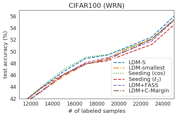
(c)

Figure 12: The effect of diverse sampling in LDM-S on MNIST (a), CIFAR10 (b), and CIFAR100 (c) datasets. ‘LDM-smallest’: selecting batch with the smallest LDM, ‘Seeding (cos)’: unweighted seeding using cosine distance, ‘Seeding ($\ell_{2}$)’: unweighted seeding using $\ell_{2}$-distance, ‘LDM+FASS’: the combination of LDM and FASS, ‘LDM+C-Margin’: the combination of LDM and Cluster-Margin. LDM-S leads to significant performance improvement compared to those without batch diversity, with FASS, or with Cluster-Margin.

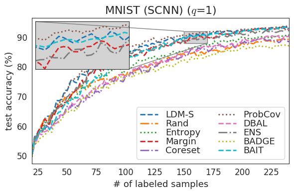
(a)

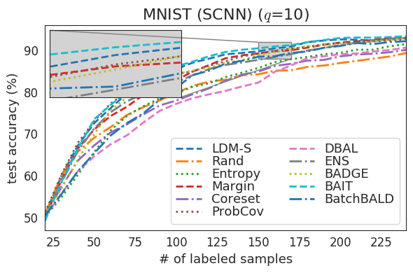
(b)

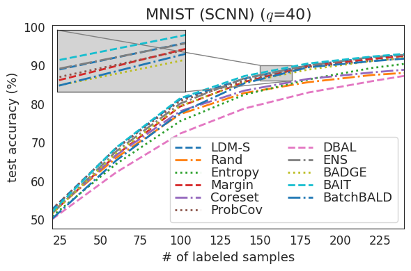
(c)

Figure 13: Performance comparison when the batch sizes are 1 (a), 10 (b), and 40 (c) on MNIST.

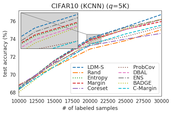
(a)

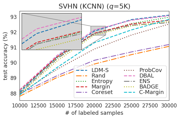
(b)

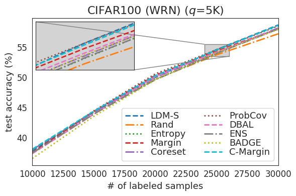
(c)

Figure 14: Performance comparison when the batch size is 5K on CIFAR10 (a), SVHN (b), and CIFAR100 (c).

F.3 Effect of Batch Size

To verify the effectiveness of LDM-S for batch mode, we compare the active learning performance with respect to various batch sizes. Figure 13 shows the test accuracy when the batch sizes are 1, 10, and 40 on the MNIST dataset. Figure 14 shows the test accuracy when the batch size is 5K on CIFAR10, SVHM, and CIFAR100 datasets. Overall, LDM-S performs well compared to other algorithms, even with small and large batch sizes. Therefore, the proposed algorithm is robust to the batch size, while other baseline algorithms often do not, e.g., BADGE performs well with batch size 10 or 40 but is poor with batch size 1 on MNIST. Note that we have added additional results for BatchBALD in Figure 13 and Cluster-Margin (C-Margin) in Figure 14. For both settings, we’ve matched the setting as described in their original papers.

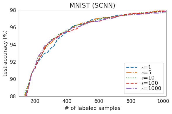
(a)

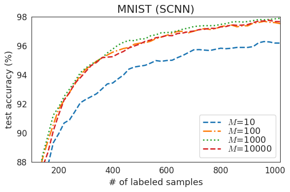
(b)

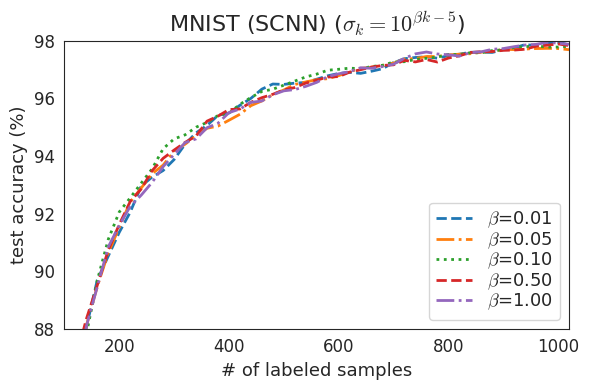
(c)

Figure 15: Performance vs hyperparameters. The test accuracy with respect to stop condition $s$ (a), the number of Monte Carlo samples for approximating $\rho$ (b), and sigmas’ interval (c).

F.4 Effect of Hyperparameters in LDM-S

There are three hyperparameters in the proposed algorithm: stop condition $s$, the number of Monte Carlo samples $M$, and the set of variances $\{\sigma_{k}^{2}\}_{k=1}^{K}$.

The stop condition $s$ is required for LDM evaluation. We set $s=10$, considering the rank correlation coefficient and computing time. Figure 15a shows the test accuracy with respect to $s\in\{1,5,10,100,1000\}$, and there is no significant performance difference.

The number of Monte Carlo samples $M$ is set for approximating $\rho$. The proposed algorithm aims to distinguish LDMs of pool data, thus, we set $M$ to be the same size as the pool size. Figure 15b shows the test accuracy with respect to $M\in\{10,100,1000,10000\}$, and there is no significant performance difference except where $M$ is extremely small, e.g., $M=10$.

The set of variances $\{\sigma_{k}^{2}\}_{k=1}^{K}$ is set for hypothesis sampling. Figure 7 in Appendix C.2 shows the relationship between the disagree metric and $\sigma^{2}$. To properly approximate LDM, we need to sample hypotheses with a wide range of $\rho$, and thus we need a wide range of $\sigma^{2}$. To efficiently cover a wide range of $\sigma^{2}$, we make the exponent equally spaced such as $\sigma_{k}=10^{\beta k-5}$ where $\beta>0$ and set $\sigma$ the have $10^{-5}$ to $1$. Figure 15c shows the test accuracy with respect to $\beta\in\{0.01,0.05,0.1,0.5,1\}$, and there is no significant performance difference.

Appendix G Additional Results

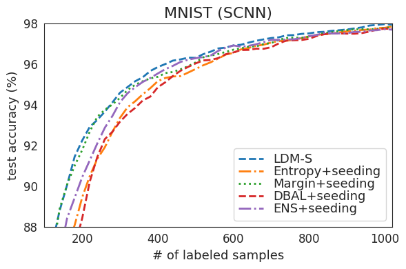
(a)

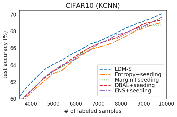
(b)

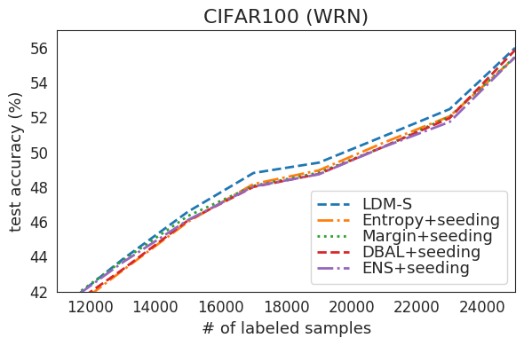
(c)

Figure 16: The performance comparison of LDM-S with the standard uncertainty methods to which weighted seeding is applied on MNIST (a), CIFAR10 (b), and CIFAR100 (c). Even if weighted seeding is applied to the standard uncertainty methods, LDM-S performs better.

G.1 Comparing with Other Uncertainty Methods with Seeding

To clarify whether the gains of LDM-S over the standard uncertainty methods are due to weighted seeding or due to the superiority of LDM, the performance of LDM-S is compared with those methods to which weighted seeding is applied. Figure 16 shows the test accuracy with respect to the number of labeled samples on MNIST, CIFAR10, and CIFAR100 datasets. Overall, even when weighted seeding is applied to the standard uncertainty methods, LDM-S still performs better on all datasets. Therefore, the performance gains of LDM-S can be attributed to LDM’s superiority over the standard uncertainty measures.

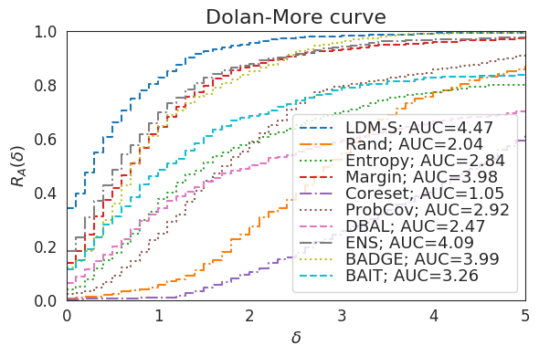
(a)

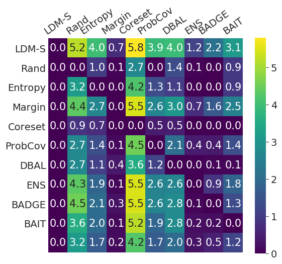
(b)

Figure 17: Comparison with BAIT across OpenML #6, #156, #44135, MNIST, CIFAR10, and SVHN datasets. (a) Dolan-Moré plot. (b) The penalty matrix.

G.2 Comparison across Datasets with BAIT

The performance profile and penalty matrix between LDM-S and BAIT, are examined on OpenML #6, #156, #44135, MNIST, CIFAR10, and SVHN datasets where the experiments for BAIT are conducted. Figure 17a shows the performance profile w.r.t. $\delta$. It is clear that LDM-S retains the highest $R_{A}(\delta)$ over all considered $\delta$’s, which means that our LDM-S outperforms the other algorithms including BAIT. Figure 17b shows the penalty matrix. It is, also, clear that LDM-S generally outperforms all other algorithms including BAIT.

G.3 Comparison per Datasets

Table LABEL:tbl:openml6 shows the mean $\pm$ std of the test accuracies (%) w.r.t. the number of labeled samples for OpenML #6, #156, #44135 with MLP; MNIST with SCNN; CIFAR10 and SVHN with K-CNN; CIFAR100, Tiny ImageNet, FOOD101 with WRN-16-8; and ImageNet with ResNet-18. Overall, LDM-S either consistently performs best or is at par with other algorithms for all datasets, while the performance of the algorithms except LDM-S varies depending on datasets.

Table 5: The mean $\pm$ std of the test accuracies (%) w.r.t. the number of labeled samples. (bold+underlined: best performance, bold: second-best performance)

$|\mathcal{L}|$	LDM-S	Rand	Entropy	Margin	Coreset	ProbCov	DBAL	ENS	BADGE	BAIT
OpenML#6
400	62.42 ± 0.01	60.64 ± 0.01	56.92 ± 0.01	61.22 ± 0.03	61.23 ± 0.02	61.00 ± 0.01	58.64 ± 0.02	60.96 ± 0.02	61.65 ± 0.01	61.43 ± 0.01
800	76.29 ± 0.01	72.51 ± 0.00	66.38 ± 0.01	74.94 ± 0.01	73.66 ± 0.01	73.10 ± 0.00	70.59 ± 0.01	75.53 ± 0.01	75.13 ± 0.01	73.55 ± 0.00
1,200	81.62 ± 0.01	77.49 ± 0.00	70.62 ± 0.02	80.57 ± 0.00	78.64 ± 0.01	77.71 ± 0.01	75.98 ± 0.01	81.30 ± 0.01	79.85 ± 0.01	78.52 ± 0.01
1,600	84.74 ± 0.00	80.20 ± 0.00	73.61 ± 0.02	83.91 ± 0.01	81.26 ± 0.01	80.15 ± 0.01	79.07 ± 0.00	84.24 ± 0.01	82.60 ± 0.00	81.84 ± 0.00
2,000	87.05 ± 0.00	82.06 ± 0.00	77.49 ± 0.02	86.41 ± 0.00	83.17 ± 0.01	82.21 ± 0.01	81.73 ± 0.00	86.82 ± 0.00	84.81 ± 0.00	84.39 ± 0.01
2,400	89.12 ± 0.00	83.62 ± 0.01	81.80 ± 0.01	88.59 ± 0.01	85.00 ± 0.01	84.01 ± 0.01	84.20 ± 0.01	88.74 ± 0.01	87.04 ± 0.00	86.73 ± 0.01
2,800	90.35 ± 0.00	84.77 ± 0.01	85.12 ± 0.01	89.76 ± 0.00	86.22 ± 0.00	85.04 ± 0.00	86.00 ± 0.01	90.10 ± 0.01	88.31 ± 0.00	88.44 ± 0.00
3,200	91.06 ± 0.00	85.96 ± 0.01	87.37 ± 0.00	90.83 ± 0.00	87.22 ± 0.00	85.95 ± 0.00	87.43 ± 0.01	90.96 ± 0.00	89.18 ± 0.00	89.76 ± 0.00
3,600	91.80 ± 0.00	86.77 ± 0.00	88.57 ± 0.00	91.50 ± 0.00	87.85 ± 0.01	86.90 ± 0.01	88.83 ± 0.00	91.70 ± 0.00	90.21 ± 0.00	90.57 ± 0.00
4,000	92.53 ± 0.00	88.00 ± 0.01	89.54 ± 0.00	92.36 ± 0.00	88.49 ± 0.01	87.72 ± 0.00	89.69 ± 0.00	92.62 ± 0.00	91.35 ± 0.00	91.28 ± 0.00
OpenML#156
200	69.78 ± 0.02	70.30 ± 0.02	65.23 ± 0.02	67.95 ± 0.03	61.15 ± 0.03	70.02 ± 0.01	64.10 ± 0.04	67.97 ± 0.02	71.35 ± 0.02	67.62 ± 0.03
400	83.08 ± 0.02	83.27 ± 0.01	76.42 ± 0.03	81.58 ± 0.02	63.92 ± 0.03	82.68 ± 0.01	70.78 ± 0.01	82.19 ± 0.02	83.74 ± 0.02	76.04 ± 0.02
600	87.30 ± 0.01	86.20 ± 0.01	83.11 ± 0.01	86.75 ± 0.01	65.46 ± 0.04	85.65 ± 0.00	72.06 ± 0.02	86.38 ± 0.01	86.68 ± 0.01	77.68 ± 0.01
800	88.60 ± 0.00	87.09 ± 0.00	85.95 ± 0.01	88.14 ± 0.00	65.40 ± 0.05	86.79 ± 0.00	72.88 ± 0.02	88.17 ± 0.00	87.97 ± 0.00	78.47 ± 0.02
1,000	89.32 ± 0.00	87.63 ± 0.01	87.65 ± 0.01	88.83 ± 0.00	65.59 ± 0.05	87.56 ± 0.01	72.82 ± 0.02	89.21 ± 0.00	88.94 ± 0.00	78.89 ± 0.01
1,200	90.08 ± 0.00	88.31 ± 0.00	89.13 ± 0.00	89.83 ± 0.00	67.90 ± 0.05	88.51 ± 0.00	72.55 ± 0.03	89.88 ± 0.00	89.59 ± 0.00	79.29 ± 0.01
1,400	90.43 ± 0.00	88.78 ± 0.00	89.88 ± 0.00	90.40 ± 0.00	69.14 ± 0.02	89.03 ± 0.00	72.87 ± 0.02	90.23 ± 0.00	89.99 ± 0.00	80.45 ± 0.01
1,600	90.70 ± 0.00	89.11 ± 0.00	90.14 ± 0.00	90.67 ± 0.00	70.02 ± 0.04	89.46 ± 0.00	73.06 ± 0.01	90.48 ± 0.00	90.28 ± 0.00	80.70 ± 0.01
1,800	90.95 ± 0.00	89.42 ± 0.00	90.37 ± 0.00	90.85 ± 0.00	70.03 ± 0.05	89.69 ± 0.00	73.96 ± 0.02	90.75 ± 0.00	90.49 ± 0.00	81.85 ± 0.02
2,000	91.19 ± 0.00	89.67 ± 0.00	90.62 ± 0.00	91.09 ± 0.00	70.92 ± 0.05	90.05 ± 0.00	73.92 ± 0.03	91.01 ± 0.00	90.73 ± 0.00	84.17 ± 0.02
OpenML#44135
200	82.28 ± 0.01	77.44 ± 0.02	75.67 ± 0.01	81.33 ± 0.01	75.92 ± 0.00	81.70 ± 0.01	76.56 ± 0.02	78.16 ± 0.02	78.33 ± 0.01	78.82 ± 0.01
400	92.65 ± 0.01	86.21 ± 0.01	86.18 ± 0.02	92.10 ± 0.00	84.92 ± 0.01	91.59 ± 0.01	86.56 ± 0.01	88.60 ± 0.00	88.60 ± 0.00	89.50 ± 0.01
600	94.51 ± 0.00	89.18 ± 0.01	91.17 ± 0.01	94.12 ± 0.00	89.48 ± 0.01	93.51 ± 0.00	90.63 ± 0.00	92.18 ± 0.00	92.06 ± 0.01	92.29 ± 0.00
800	95.34 ± 0.01	91.05 ± 0.01	93.26 ± 0.00	95.30 ± 0.00	91.29 ± 0.01	94.69 ± 0.00	92.65 ± 0.00	93.70 ± 0.01	93.42 ± 0.00	93.49 ± 0.01
1,000	95.86 ± 0.00	91.90 ± 0.00	94.41 ± 0.00	96.03 ± 0.00	92.47 ± 0.00	95.02 ± 0.01	93.78 ± 0.00	94.82 ± 0.01	94.28 ± 0.01	94.41 ± 0.01
1,200	96.13 ± 0.00	92.35 ± 0.00	95.13 ± 0.00	96.28 ± 0.00	93.03 ± 0.00	95.22 ± 0.00	94.57 ± 0.01	95.29 ± 0.01	95.12 ± 0.00	94.87 ± 0.00
1,400	96.27 ± 0.00	92.81 ± 0.00	95.62 ± 0.00	96.38 ± 0.00	93.61 ± 0.00	95.57 ± 0.00	95.26 ± 0.00	95.53 ± 0.01	95.53 ± 0.00	95.43 ± 0.00
1,600	96.51 ± 0.00	93.29 ± 0.00	95.93 ± 0.00	96.44 ± 0.01	94.18 ± 0.01	95.73 ± 0.00	95.48 ± 0.00	95.58 ± 0.00	95.88 ± 0.01	95.64 ± 0.01
1,800	96.60 ± 0.00	93.42 ± 0.01	95.84 ± 0.01	96.38 ± 0.00	94.41 ± 0.00	95.79 ± 0.00	95.63 ± 0.00	95.72 ± 0.01	95.98 ± 0.00	95.84 ± 0.00
2,000	96.62 ± 0.00	93.73 ± 0.01	96.40 ± 0.00	96.21 ± 0.00	94.59 ± 0.00	95.96 ± 0.01	96.21 ± 0.00	96.13 ± 0.00	96.26 ± 0.00	95.65 ± 0.00
MNIST
120	87.08 ± 0.01	81.32 ± 0.02	80.67 ± 0.04	84.86 ± 0.01	79.29 ± 0.03	86.61 ± 0.01	78.59 ± 0.01	85.34 ± 0.01	85.43 ± 0.02	87.07 ± 0.01
220	92.92 ± 0.00	88.08 ± 0.01	90.83 ± 0.01	92.17 ± 0.01	87.37 ± 0.02	92.44 ± 0.01	88.43 ± 0.01	91.70 ± 0.01	92.53 ± 0.01	92.99 ± 0.01
320	94.88 ± 0.00	90.99 ± 0.01	93.95 ± 0.00	94.67 ± 0.00	90.90 ± 0.02	94.30 ± 0.00	93.03 ± 0.00	94.30 ± 0.00	94.68 ± 0.00	94.93 ± 0.00
420	96.01 ± 0.00	92.45 ± 0.01	95.35 ± 0.00	95.87 ± 0.00	92.84 ± 0.02	95.43 ± 0.00	95.22 ± 0.00	95.82 ± 0.00	95.64 ± 0.01	96.09 ± 0.00
520	96.50 ± 0.00	93.51 ± 0.01	96.00 ± 0.00	96.34 ± 0.00	93.70 ± 0.01	96.13 ± 0.00	95.80 ± 0.00	96.46 ± 0.00	96.33 ± 0.00	96.64 ± 0.00
620	96.96 ± 0.00	94.22 ± 0.00	96.78 ± 0.00	96.93 ± 0.00	94.77 ± 0.01	96.63 ± 0.00	96.80 ± 0.00	96.94 ± 0.00	96.82 ± 0.00	97.11 ± 0.00
720	97.33 ± 0.00	94.78 ± 0.00	97.12 ± 0.00	97.15 ± 0.00	95.21 ± 0.01	96.98 ± 0.00	96.95 ± 0.00	97.36 ± 0.00	97.02 ± 0.00	97.28 ± 0.00
820	97.58 ± 0.00	95.18 ± 0.00	97.41 ± 0.00	97.46 ± 0.00	95.38 ± 0.01	97.06 ± 0.00	97.31 ± 0.00	97.56 ± 0.00	97.46 ± 0.00	97.49 ± 0.00
920	97.77 ± 0.00	95.44 ± 0.00	97.69 ± 0.00	97.68 ± 0.00	95.97 ± 0.00	97.44 ± 0.00	97.51 ± 0.00	97.63 ± 0.00	97.61 ± 0.00	97.65 ± 0.00
1,020	97.95 ± 0.00	95.88 ± 0.00	97.88 ± 0.00	97.84 ± 0.00	95.84 ± 0.01	97.63 ± 0.00	97.77 ± 0.00	97.75 ± 0.00	97.78 ± 0.00	97.97 ± 0.00
CIFAR10
1,400	50.30 ± 0.00	49.16 ± 0.01	48.96 ± 0.01	49.35 ± 0.01	47.44 ± 0.01	49.46 ± 0.01	49.51 ± 0.01	49.93 ± 0.01	50.23 ± 0.01	49.48 ± 0.00
2,600	57.01 ± 0.01	56.04 ± 0.01	55.35 ± 0.01	56.51 ± 0.01	52.95 ± 0.01	56.09 ± 0.01	55.53 ± 0.01	56.39 ± 0.01	56.74 ± 0.01	56.35 ± 0.01
3,800	61.30 ± 0.01	59.99 ± 0.00	59.68 ± 0.01	60.49 ± 0.00	56.30 ± 0.01	59.99 ± 0.00	59.43 ± 0.01	60.34 ± 0.01	60.54 ± 0.01	60.39 ± 0.01
5,000	64.09 ± 0.00	62.69 ± 0.01	62.60 ± 0.00	62.81 ± 0.01	58.70 ± 0.00	62.73 ± 0.01	62.31 ± 0.00	63.32 ± 0.00	63.93 ± 0.01	63.00 ± 0.00
6,200	65.79 ± 0.00	64.56 ± 0.01	64.42 ± 0.00	64.97 ± 0.00	61.08 ± 0.01	64.38 ± 0.01	64.00 ± 0.01	64.99 ± 0.01	65.30 ± 0.00	65.32 ± 0.00
7,400	67.28 ± 0.01	65.87 ± 0.00	66.29 ± 0.00	66.75 ± 0.01	62.84 ± 0.01	66.28 ± 0.01	66.12 ± 0.01	66.78 ± 0.01	67.11 ± 0.01	66.82 ± 0.01
8,600	68.83 ± 0.00	67.50 ± 0.01	67.77 ± 0.01	67.87 ± 0.01	63.50 ± 0.01	67.60 ± 0.00	67.94 ± 0.01	68.11 ± 0.01	68.42 ± 0.00	67.99 ± 0.00
9,800	70.10 ± 0.00	68.51 ± 0.01	68.62 ± 0.00	69.13 ± 0.01	64.44 ± 0.01	68.45 ± 0.00	68.82 ± 0.01	69.23 ± 0.01	69.08 ± 0.00	69.42 ± 0.01
SVHN
1,400	79.02 ± 0.01	77.22 ± 0.01	76.25 ± 0.01	77.94 ± 0.01	75.84 ± 0.01	77.56 ± 0.01	78.42 ± 0.01	77.49 ± 0.01	78.31 ± 0.01	77.91 ± 0.00
2,600	83.76 ± 0.00	81.55 ± 0.01	82.33 ± 0.00	83.61 ± 0.01	80.62 ± 0.01	82.55 ± 0.01	83.27 ± 0.01	83.23 ± 0.01	83.49 ± 0.00	83.13 ± 0.00
3,800	86.08 ± 0.00	83.61 ± 0.00	85.33 ± 0.00	85.28 ± 0.01	81.95 ± 0.01	84.59 ± 0.00	86.00 ± 0.00	85.85 ± 0.01	85.68 ± 0.00	85.54 ± 0.00
5,000	87.58 ± 0.00	85.05 ± 0.00	86.78 ± 0.00	87.11 ± 0.00	83.12 ± 0.00	85.92 ± 0.00	87.49 ± 0.00	87.23 ± 0.00	87.32 ± 0.01	87.49 ± 0.00
6,200	88.64 ± 0.00	85.98 ± 0.00	88.09 ± 0.00	88.11 ± 0.00	84.21 ± 0.00	86.89 ± 0.00	88.91 ± 0.00	88.30 ± 0.00	88.38 ± 0.00	88.61 ± 0.01
7,400	89.56 ± 0.00	86.59 ± 0.00	88.84 ± 0.00	89.03 ± 0.00	84.73 ± 0.00	87.57 ± 0.00	89.61 ± 0.00	89.31 ± 0.01	89.20 ± 0.00	89.29 ± 0.00
8,600	90.04 ± 0.00	87.28 ± 0.00	89.65 ± 0.00	89.62 ± 0.00	85.25 ± 0.00	88.22 ± 0.00	90.34 ± 0.00	90.04 ± 0.00	89.90 ± 0.00	90.07 ± 0.00
9,800	90.61 ± 0.00	87.72 ± 0.00	90.16 ± 0.00	90.45 ± 0.00	86.13 ± 0.00	88.80 ± 0.00	90.77 ± 0.00	90.32 ± 0.00	90.10 ± 0.00	90.52 ± 0.00
CIFAR100
7,000	31.85 ± 0.00	31.28 ± 0.01	30.74 ± 0.01	31.18 ± 0.01	31.46 ± 0.01	31.76 ± 0.01	30.80 ± 0.01	31.09 ± 0.01	30.89 ± 0.00	-
9,000	37.61 ± 0.00	36.94 ± 0.01	36.30 ± 0.00	36.83 ± 0.02	37.60 ± 0.01	37.68 ± 0.01	36.32 ± 0.01	36.42 ± 0.00	36.69 ± 0.01
11,000	40.88 ± 0.01	40.40 ± 0.02	39.91 ± 0.01	40.33 ± 0.01	41.33 ± 0.01	41.43 ± 0.01	40.24 ± 0.01	40.04 ± 0.00	40.34 ± 0.01
13,000	43.86 ± 0.01	43.13 ± 0.00	43.16 ± 0.01	43.51 ± 0.01	44.15 ± 0.00	44.02 ± 0.01	43.32 ± 0.01	42.80 ± 0.01	43.44 ± 0.01
15,000	46.59 ± 0.01	45.77 ± 0.01	45.77 ± 0.01	46.10 ± 0.00	46.58 ± 0.01	46.55 ± 0.01	46.11 ± 0.01	45.53 ± 0.01	46.20 ± 0.01
17,000	48.81 ± 0.01	47.75 ± 0.01	47.86 ± 0.01	48.36 ± 0.00	48.69 ± 0.01	48.24 ± 0.01	48.23 ± 0.01	47.58 ± 0.01	48.46 ± 0.00
19,000	49.41 ± 0.01	48.35 ± 0.01	48.66 ± 0.00	48.96 ± 0.01	49.28 ± 0.01	48.82 ± 0.01	48.99 ± 0.01	48.52 ± 0.01	49.20 ± 0.01
21,000	50.94 ± 0.00	49.87 ± 0.01	50.49 ± 0.01	50.56 ± 0.01	50.71 ± 0.01	50.34 ± 0.00	50.60 ± 0.01	50.10 ± 0.01	50.54 ± 0.01
23,000	52.48 ± 0.00	51.29 ± 0.01	52.10 ± 0.01	52.04 ± 0.01	51.93 ± 0.00	52.02 ± 0.00	52.29 ± 0.00	51.74 ± 0.01	52.06 ± 0.01
25,000	56.00 ± 0.00	54.51 ± 0.01	55.73 ± 0.01	55.52 ± 0.00	55.15 ± 0.01	55.70 ± 0.01	55.72 ± 0.01	55.03 ± 0.01	55.63 ± 0.01
Tiny ImageNet
15,000	23.97 ± 0.00	23.72 ± 0.01	23.13 ± 0.00	23.80 ± 0.01	23.87 ± 0.01	24.06 ± 0.00	23.71 ± 0.01	23.23 ± 0.01	23.70 ± 0.01	-
20,000	27.76 ± 0.00	27.65 ± 0.00	26.72 ± 0.00	27.39 ± 0.01	27.67 ± 0.01	28.22 ± 0.01	27.70 ± 0.01	27.29 ± 0.01	27.65 ± 0.00
25,000	31.51 ± 0.01	31.22 ± 0.00	30.30 ± 0.01	30.90 ± 0.00	31.18 ± 0.00	31.64 ± 0.01	31.30 ± 0.01	30.82 ± 0.01	31.21 ± 0.00
30,000	34.39 ± 0.01	34.23 ± 0.01	33.38 ± 0.01	33.72 ± 0.00	33.85 ± 0.01	34.54 ± 0.01	34.27 ± 0.01	33.73 ± 0.00	34.20 ± 0.00
35,000	37.43 ± 0.01	36.77 ± 0.01	36.16 ± 0.00	36.78 ± 0.00	36.38 ± 0.01	36.79 ± 0.01	36.88 ± 0.00	36.11 ± 0.01	36.88 ± 0.01
40,000	39.39 ± 0.01	38.59 ± 0.01	38.34 ± 0.00	39.51 ± 0.01	38.36 ± 0.01	39.02 ± 0.02	39.08 ± 0.01	38.43 ± 0.01	38.90 ± 0.01
45,000	41.32 ± 0.01	40.25 ± 0.02	40.04 ± 0.01	41.50 ± 0.00	39.97 ± 0.01	40.73 ± 0.00	40.92 ± 0.02	40.73 ± 0.01	40.70 ± 0.01
50,000	42.65 ± 0.01	41.73 ± 0.01	41.40 ± 0.01	43.01 ± 0.01	41.16 ± 0.02	42.70 ± 0.01	42.59 ± 0.02	42.90 ± 0.01	42.01 ± 0.01
FOOD101
9,000	26.32 ± 0.00	25.86 ± 0.01	25.42 ± 0.00	25.63 ± 0.01	26.49 ± 0.01	25.91 ± 0.00	26.06 ± 0.01	25.54 ± 0.00	25.55 ± 0.01	-
12,000	30.83 ± 0.01	29.89 ± 0.01	29.10 ± 0.00	29.77 ± 0.01	31.03 ± 0.00	30.40 ± 0.00	30.44 ± 0.01	29.56 ± 0.01	29.83 ± 0.01
15,000	35.08 ± 0.01	34.19 ± 0.00	33.01 ± 0.01	34.31 ± 0.01	35.40 ± 0.01	34.70 ± 0.01	35.12 ± 0.01	33.71 ± 0.01	34.32 ± 0.01
18,000	38.50 ± 0.01	37.15 ± 0.01	36.18 ± 0.01	37.68 ± 0.01	38.62 ± 0.01	38.00 ± 0.01	38.48 ± 0.00	36.82 ± 0.01	37.88 ± 0.01
21,000	42.26 ± 0.01	40.74 ± 0.00	39.71 ± 0.01	41.53 ± 0.01	42.37 ± 0.01	41.60 ± 0.01	42.16 ± 0.01	40.66 ± 0.01	41.69 ± 0.01
24,000	45.46 ± 0.01	43.81 ± 0.01	43.24 ± 0.01	44.48 ± 0.01	45.24 ± 0.01	44.58 ± 0.01	45.20 ± 0.01	43.93 ± 0.01	45.17 ± 0.01
27,000	48.88 ± 0.00	47.37 ± 0.01	46.64 ± 0.01	47.75 ± 0.01	48.70 ± 0.01	47.67 ± 0.00	48.69 ± 0.01	47.49 ± 0.00	48.39 ± 0.01
30,000	51.40 ± 0.00	50.24 ± 0.00	49.67 ± 0.01	50.20 ± 0.00	51.22 ± 0.00	49.72 ± 0.01	51.52 ± 0.01	50.12 ± 0.01	50.93 ± 0.01
ImageNet
192,180	41.99 ± 0.00	41.45 ± 0.01	41.25 ± 0.00	41.62 ± 0.01	41.27 ± 0.00	41.90 ± 0.01	-	41.92 ± 0.00	41.90 ± 0.01	-
256,240	46.62 ± 0.00	45.90 ± 0.00	45.58 ± 0.01	46.01 ± 0.01	45.41 ± 0.00	46.33 ± 0.00		46.49 ± 0.01	46.52 ± 0.01
320,300	50.14 ± 0.00	49.08 ± 0.01	48.86 ± 0.01	49.26 ± 0.01	48.38 ± 0.01	49.33 ± 0.01		49.72 ± 0.01	49.88 ± 0.01
384,360	53.53 ± 0.00	52.11 ± 0.00	52.18 ± 0.00	52.16 ± 0.01	50.96 ± 0.00	51.86 ± 0.00		52.46 ± 0.00	52.95 ± 0.01

References

- Aldous (2022) David J. Aldous. Covering a compact space by fixed-radius or growing random balls. Latin American Journal of Probability and Mathematical Statistics, 19:755–767, 2022.
- Arthur & Vassilvitskii (2007) David Arthur and Sergei Vassilvitskii. K-Means++: The Advantages of Careful Seeding. In Proceedings of the Eighteenth Annual ACM-SIAM Symposium on Discrete Algorithms, SODA ’07, pp. 1027–1035, USA, 2007. Society for Industrial and Applied Mathematics.
- Ash et al. (2021) Jordan Ash, Surbhi Goel, Akshay Krishnamurthy, and Sham Kakade. Gone Fishing: Neural Active Learning with Fisher Embeddings. In Advances in Neural Information Processing Systems, volume 34, pp. 8927–8939. Curran Associates, Inc., 2021.
- Ash et al. (2020) Jordan T. Ash, Chicheng Zhang, Akshay Krishnamurthy, John Langford, and Alekh Agarwal. Deep Batch Active Learning by Diverse, Uncertain Gradient Lower Bounds. In International Conference on Learning Representations, 2020.
- Auer et al. (2002) Peter Auer, Nicolo Cesa-Bianchi, Yoav Freund, and Robert E Schapire. The nonstochastic multiarmed bandit problem. SIAM Journal on Computing, 32(1):48–77, 2002.
- Balcan et al. (2007) Maria-Florina Balcan, Andrei Broder, and Tong Zhang. Margin based active learning. In Nader H. Bshouty and Claudio Gentile (eds.), Learning Theory – COLT 2007, pp. 35–50, Berlin, Heidelberg, 2007. Springer Berlin Heidelberg.
- Beluch et al. (2018) William H. Beluch, Tim Genewein, Andreas Nurnberger, and Jan M. Kohler. The Power of Ensembles for Active Learning in Image Classification. In 2018 IEEE/CVF Conference on Computer Vision and Pattern Recognition, pp. 9368–9377, 2018.
- Beygelzimer et al. (2009) Alina Beygelzimer, Sanjoy Dasgupta, and John Langford. Importance Weighted Active Learning. In Proceedings of the 26th Annual International Conference on Machine Learning, ICML ’09, pp. 49–56, New York, NY, USA, 2009. Association for Computing Machinery.
- Bossard et al. (2014) Lukas Bossard, Matthieu Guillaumin, and Luc Van Gool. Food-101 – mining discriminative components with random forests. In Computer Vision – ECCV 2014, pp. 446–461, Cham, 2014. Springer International Publishing.
- Box & Muller (1958) G. E. P. Box and Mervin E. Muller. A Note on the Generation of Random Normal Deviates. The Annals of Mathematical Statistics, 29(2):610 – 611, 1958.
- Burnaev et al. (2015a) E. Burnaev, P. Erofeev, and A. Papanov. Influence of resampling on accuracy of imbalanced classification. In Eighth International Conference on Machine Vision (ICMV 2015), volume 9875, pp. 987521. International Society for Optics and Photonics, SPIE, 2015a.
- Burnaev et al. (2015b) E. Burnaev, P. Erofeev, and D. Smolyakov. Model selection for anomaly detection. In Eighth International Conference on Machine Vision (ICMV 2015), volume 9875, pp. 987525. International Society for Optics and Photonics, SPIE, 2015b.
- Caramalau et al. (2021) Razvan Caramalau, Binod Bhattarai, and Tae-Kyun Kim. Sequential Graph Convolutional Network for Active Learning. In 2021 IEEE/CVF Conference on Computer Vision and Pattern Recognition (CVPR), pp. 9578–9587, 2021.
- Chaudhari & Soatto (2018) Pratik Chaudhari and Stefano Soatto. Stochastic gradient descent performs variational inference, converges to limit cycles for deep networks. In International Conference on Learning Representations, 2018.
- Chollet et al. (2015) François Chollet et al. Keras. https://keras.io, 2015.
- Citovsky et al. (2021) Gui Citovsky, Giulia DeSalvo, Claudio Gentile, Lazaros Karydas, Anand Rajagopalan, Afshin Rostamizadeh, and Sanjiv Kumar. Batch Active Learning at Scale. In Advances in Neural Information Processing Systems, volume 34, pp. 11933–11944. Curran Associates, Inc., 2021.
- Cohn et al. (1996) David A. Cohn, Zoubin Ghahramani, and Michael I. Jordan. Active Learning with Statistical Models. Journal of Artificial Intelligence Research, 4(1):129–145, Mar 1996.
- Dasgupta (2011) Sanjoy Dasgupta. Two faces of active learning. Theoretical Computer Science, 412(19):1767–1781, 2011. Algorithmic Learning Theory (ALT 2009).
- Dolan & Moré (2002) Elizabeth D. Dolan and Jorge J. Moré. Benchmarking optimization software with performance profiles. Mathematical Programming, 91(2):201–213, Jan 2002.
- Ducoffe & Precioso (2018) Melanie Ducoffe and Frederic Precioso. Adversarial Active Learning for Deep Networks: a Margin Based Approach. arXiv preprint arXiv:1802.09841, 2018.
- Dudley (2002) R. M. Dudley. Real Analysis and Probability. Cambridge Series in Advanced Mathematics. Cambridge University Press, 2002.
- Elenter et al. (2022) Juan Elenter, Navid Naderializadeh, and Alejandro Ribeiro. A Lagrangian Duality Approach to Active Learning. In Advances in Neural Information Processing Systems, volume 35, pp. 37575–37589. Curran Associates, Inc., 2022.
- Fanty & Cole (1990) Mark Fanty and Ronald Cole. Spoken Letter Recognition. In Advances in Neural Information Processing Systems, volume 3. Morgan-Kaufmann, 1990.
- Frey & Slate (1991) Peter W Frey and David J Slate. Letter recognition using Holland-style adaptive classifiers. Machine learning, 6(2):161–182, 1991.
- Freytag et al. (2014) Alexander Freytag, Erik Rodner, and Joachim Denzler. Selecting influential examples: Active learning with expected model output changes. In Computer Vision – ECCV 2014, pp. 562–577, Cham, 2014. Springer International Publishing.
- Gal & Ghahramani (2016) Yarin Gal and Zoubin Ghahramani. Dropout as a Bayesian Approximation: Representing Model Uncertainty in Deep Learning. In Proceedings of The 33rd International Conference on Machine Learning, volume 48 of Proceedings of Machine Learning Research, pp. 1050–1059, New York, New York, USA, 20–22 Jun 2016. PMLR.
- Gal et al. (2017) Yarin Gal, Riashat Islam, and Zoubin Ghahramani. Deep Bayesian Active Learning with Image Data. In Proceedings of the 34th International Conference on Machine Learning, volume 70 of Proceedings of Machine Learning Research, pp. 1183–1192. PMLR, 06–11 Aug 2017.
- Ganti & Gray (2012) Ravi Ganti and Alexander Gray. UPAL: Unbiased Pool Based Active Learning. In Proceedings of the Fifteenth International Conference on Artificial Intelligence and Statistics, volume 22 of Proceedings of Machine Learning Research, pp. 422–431, La Palma, Canary Islands, 21–23 Apr 2012. PMLR.
- Gu et al. (2021) Bin Gu, Zhou Zhai, Cheng Deng, and Heng Huang. Efficient Active Learning by Querying Discriminative and Representative Samples and Fully Exploiting Unlabeled Data. IEEE Transactions on Neural Networks and Learning Systems, 32(9):4111–4122, 2021.
- Hanneke (2014) Steve Hanneke. Theory of Disagreement-Based Active Learning. Foundations and Trends® in Machine Learning, 7(2-3):131–309, 2014.
- He et al. (2015) Kaiming He, Xiangyu Zhang, Shaoqing Ren, and Jian Sun. Delving Deep into Rectifiers: Surpassing Human-Level Performance on ImageNet Classification. In 2015 IEEE International Conference on Computer Vision (ICCV), pp. 1026–1034, 2015.
- He et al. (2016) Kaiming He, Xiangyu Zhang, Shaoqing Ren, and Jian Sun. Deep Residual Learning for Image Recognition. In 2016 IEEE Conference on Computer Vision and Pattern Recognition (CVPR), pp. 770–778, 2016. doi: 10.1109/CVPR.2016.90.
- Hjort et al. (2010) Nils Lid Hjort, Chris Holmes, Peter Müller, and Stephen G Walker. Bayesian Nonparametrics. Number 28 in Cambridge Series in Statistical and Probabilistic Mathematics. Cambridge University Press, 2010.
- Houlsby et al. (2011) Neil Houlsby, Ferenc Huszár, Zoubin Ghahramani, and Máté Lengyel. Bayesian Active Learning for Classification and Preference Learning. arXiv preprint arXiv:1112.5745, 2011.
- Joshi et al. (2009) Ajay J. Joshi, Fatih Porikli, and Nikolaos Papanikolopoulos. Multi-class active learning for image classification. In 2009 IEEE Conference on Computer Vision and Pattern Recognition, pp. 2372–2379, 2009.
- Jung et al. (2023) Seohyeon Jung, Sanghyun Kim, and Juho Lee. A simple yet powerful deep active learning with snapshots ensembles. In The Eleventh International Conference on Learning Representations, 2023.
- Kim & Yoo (2022) Gwangsu Kim and Chang D. Yoo. Blending Query Strategy of Active Learning for Imbalanced Data. IEEE Access, 10:79526–79542, 2022.
- Kim et al. (2021) Yoon-Yeong Kim, Kyungwoo Song, JoonHo Jang, and Il-chul Moon. LADA: Look-Ahead Data Acquisition via Augmentation for Deep Active Learning. In Advances in Neural Information Processing Systems, volume 34, pp. 22919–22930. Curran Associates, Inc., 2021.
- Kirsch et al. (2019) Andreas Kirsch, Joost van Amersfoort, and Yarin Gal. BatchBALD: Efficient and Diverse Batch Acquisition for Deep Bayesian Active Learning. In Advances in Neural Information Processing Systems, volume 32. Curran Associates, Inc., 2019.
- Kirsch et al. (2023) Andreas Kirsch, Sebastian Farquhar, Parmida Atighehchian, Andrew Jesson, Frédéric Branchaud-Charron, and Yarin Gal. Stochastic Batch Acquisition: A Simple Baseline for Deep Active Learning. Transactions on Machine Learning Research, 2023. Expert Certification.
- Kpotufe et al. (2022) Samory Kpotufe, Gan Yuan, and Yunfan Zhao. Nuances in margin conditions determine gains in active learning. In International Conference on Artificial Intelligence and Statistics, pp. 8112–8126. PMLR, 2022.
- Krapivsky (2023) P L Krapivsky. Random sequential covering. Journal of Statistical Mechanics: Theory and Experiment, 2023(3):033202, mar 2023.
- Kremer et al. (2014) Jan Kremer, Kim Steenstrup Pedersen, and Christian Igel. Active learning with support vector machines. WIREs Data Mining and Knowledge Discovery, 4(4):313–326, 2014.
- Krizhevsky (2009) Alex Krizhevsky. Learning multiple layers of features from tiny images. Technical Report 0, University of Toronto, Toronto, Ontario, 2009.
- Le & Yang (2015) Ya Le and Xuan Yang. Tiny imagenet visual recognition challenge. Technical report, CS231N, Stanford University, 2015.
- Lecun et al. (1998) Y. Lecun, L. Bottou, Y. Bengio, and P. Haffner. Gradient-based learning applied to document recognition. Proceedings of the IEEE, 86(11):2278–2324, 1998.
- Lewis & Gale (1994) David D. Lewis and William A. Gale. A Sequential Algorithm for Training Text Classifiers. In SIGIR ’94, pp. 3–12, London, 1994. Springer London.
- Mahmood et al. (2022) Rafid Mahmood, Sanja Fidler, and Marc T Law. Low-Budget Active Learning via Wasserstein Distance: An Integer Programming Approach. In International Conference on Learning Representations, 2022.
- Mandt et al. (2017) Stephan Mandt, Matthew D. Hoffman, and David M. Blei. Stochastic Gradient Descent as Approximate Bayesian Inference. Journal of Machine Learning Research, 18(134):1–35, 2017.
- Massart (2000) Pascal Massart. Some applications of concentration inequalities to statistics. Annales de la Faculté des sciences de Toulouse : Mathématiques, Ser. 6, 9(2):245–303, 2000.
- Mickisch et al. (2020) David Mickisch, Felix Assion, Florens Greßner, Wiebke Günther, and Mariele Motta. Understanding the Decision Boundary of Deep Neural Networks: An Empirical Study. arXiv preprint arXiv:2002.01810, 2020.
- Mingard et al. (2021) Chris Mingard, Guillermo Valle-Pérez, Joar Skalse, and Ard A. Louis. Is SGD a Bayesian sampler? Well, almost. Journal of Machine Learning Research, 22(79):1–64, 2021.
- Mohamadi et al. (2022) Mohamad Amin Mohamadi, Wonho Bae, and Danica J Sutherland. Making Look-Ahead Active Learning Strategies Feasible with Neural Tangent Kernels. In Advances in Neural Information Processing Systems, volume 35. Curran Associates, Inc., 2022.
- Moosavi-Dezfooli et al. (2016) Seyed-Mohsen Moosavi-Dezfooli, Alhussein Fawzi, and Pascal Frossard. DeepFool: A Simple and Accurate Method to Fool Deep Neural Networks. In 2016 IEEE Conference on Computer Vision and Pattern Recognition (CVPR), pp. 2574–2582, 2016.
- Netzer et al. (2011) Yuval Netzer, Tao Wang, Adam Coates, Alessandro Bissacco, Bo Wu, and Andrew Y. Ng. Reading digits in natural images with unsupervised feature learning. In NIPS Workshop on Deep Learning and Unsupervised Feature Learning 2011, 2011.
- Nguyen et al. (2022) Vu-Linh Nguyen, Mohammad Hossein Shaker, and Eyke Hüllermeier. How to measure uncertainty in uncertainty sampling for active learning. Machine Learning, 111(1):89–122, 2022.
- Penrose (2023) Mathew D. Penrose. Random Euclidean coverage from within. Probability Theory and Related Fields, 185(3):747–814, 2023.
- Pinsler et al. (2019) Robert Pinsler, Jonathan Gordon, Eric Nalisnick, and José Miguel Hernández-Lobato. Bayesian Batch Active Learning as Sparse Subset Approximation. In Advances in Neural Information Processing Systems, volume 32. Curran Associates, Inc., 2019.
- Raj & Bach (2022) Anant Raj and Francis Bach. Convergence of Uncertainty Sampling for Active Learning. In Proceedings of the 39th International Conference on Machine Learning, volume 162 of Proceedings of Machine Learning Research, pp. 18310–18331. PMLR, 17–23 Jul 2022.
- Reznikov & Saff (2015) A. Reznikov and E. B. Saff. The Covering Radius of Randomly Distributed Points on a Manifold. International Mathematics Research Notices, 2016(19):6065–6094, 12 2015.
- Roth & Small (2006) Dan Roth and Kevin Small. Margin-based active learning for structured output spaces. In Machine Learning: ECML 2006: 17th European Conference on Machine Learning Berlin, Germany, September 18-22, 2006 Proceedings 17, pp. 413–424. Springer, 2006.
- Russakovsky et al. (2015) Olga Russakovsky, Jia Deng, Hao Su, Jonathan Krause, Sanjeev Satheesh, Sean Ma, Zhiheng Huang, Andrej Karpathy, Aditya Khosla, Michael Bernstein, Alexander C. Berg, and Li Fei-Fei. ImageNet Large Scale Visual Recognition Challenge. International Journal of Computer Vision (IJCV), 115(3):211–252, 2015. doi: 10.1007/s11263-015-0816-y.
- Sener & Savarese (2018) Ozan Sener and Silvio Savarese. Active Learning for Convolutional Neural Networks: A Core-Set Approach. In International Conference on Learning Representations, 2018.
- Settles (2009) Burr Settles. Active learning literature survey. Technical report, University of Wisconsin-Madison Department of Computer Sciences, 2009.
- Shannon (1948) C. E. Shannon. A mathematical theory of communication. The Bell System Technical Journal, 27(3):379–423, 1948.
- Sharma & Bilgic (2017) Manali Sharma and Mustafa Bilgic. Evidence-based uncertainty sampling for active learning. Data Mining and Knowledge Discovery, 31(1):164–202, Jan 2017.
- Shi & Yu (2019) Weishi Shi and Qi Yu. Integrating Bayesian and Discriminative Sparse Kernel Machines for Multi-class Active Learning. In Advances in Neural Information Processing Systems, volume 32, pp. 2285–2294. Curran Associates, Inc., 2019.
- Sinha et al. (2019) Samrath Sinha, Sayna Ebrahimi, and Trevor Darrell. Variational Adversarial Active Learning. In 2019 IEEE/CVF International Conference on Computer Vision (ICCV), pp. 5971–5980, 2019.
- Spearman (1904) C. Spearman. ”General Intelligence,” Objectively Determined and Measured. The American Journal of Psychology, 15(2):201–292, 1904.
- Tong & Chang (2001) Simon Tong and Edward Chang. Support Vector Machine Active Learning for Image Retrieval. In Proceedings of the Ninth ACM International Conference on Multimedia, MULTIMEDIA ’01, pp. 107–118, New York, NY, USA, 2001. Association for Computing Machinery.
- Tsymbalov et al. (2018) Evgenii Tsymbalov, Maxim Panov, and Alexander Shapeev. Dropout-based active learning for regression. In Analysis of Images, Social Networks and Texts, pp. 247–258, Cham, 2018. Springer International Publishing.
- Tsymbalov et al. (2019) Evgenii Tsymbalov, Sergei Makarychev, Alexander Shapeev, and Maxim Panov. Deeper Connections between Neural Networks and Gaussian Processes Speed-up Active Learning. In Proceedings of the Twenty-Eighth International Joint Conference on Artificial Intelligence, IJCAI-19, pp. 3599–3605. International Joint Conferences on Artificial Intelligence Organization, 7 2019.
- van der Maaten & Hinton (2008) Laurens van der Maaten and Geoffrey Hinton. Visualizing Data using t-SNE. Journal of Machine Learning Research, 9(86):2579–2605, 2008.
- van der Vaart (2000) Aad van der Vaart. Asymptotic statistics, volume 3 of Cambridge Series in Statistical and Probabilistic Mathematics. Cambridge university press, 2000.
- van der Vaart & Wellner (1996) Aad van der Vaart and Jon A. Wellner. Weak Convergence and Empirical Processes: With Applications to Statistics. Springer Series in Statistics (SSS). Springer New York, 1996.
- Vanschoren et al. (2014) Joaquin Vanschoren, Jan N Van Rijn, Bernd Bischl, and Luis Torgo. Openml: networked science in machine learning. ACM SIGKDD Explorations Newsletter, 15(2):49–60, 2014.
- Wainwright (2019) Martin J. Wainwright. High-Dimensional Statistics: A Non-Asymptotic Viewpoint. Number 48 in Cambridge Series in Statistical and Probabilistic Mathematics. Cambridge University Press, 2019.
- Wang et al. (2022) Haonan Wang, Wei Huang, Andrew Margenot, Hanghang Tong, and Jingrui He. Deep Active Learning by Leveraging Training Dynamics. In Advances in Neural Information Processing Systems, volume 35. Curran Associates, Inc., 2022.
- Wei et al. (2015) Kai Wei, Rishabh Iyer, and Jeff Bilmes. Submodularity in data subset selection and active learning. In International conference on machine learning, pp. 1954–1963. PMLR, 2015.
- Woo (2023) Jae Oh Woo. Active Learning in Bayesian Neural Networks with Balanced Entropy Learning Principle. In The Eleventh International Conference on Learning Representations, 2023.
- Yang et al. (2021) Yazhou Yang, Xiaoqing Yin, Yang Zhao, Jun Lei, Weili Li, and Zhe Shu. Batch Mode Active Learning Based on Multi-Set Clustering. IEEE Access, 9:51452–51463, 2021.
- Yang et al. (2015) Yi Yang, Zhigang Ma, Feiping Nie, Xiaojun Chang, and Alexander G. Hauptmann. Multi-Class Active Learning by Uncertainty Sampling with Diversity Maximization. International Journal of Computer Vision, 113(2):113–127, Jun 2015.
- Yehuda et al. (2022) Ofer Yehuda, Avihu Dekel, Guy Hacohen, and Daphna Weinshall. Active Learning Through a Covering Lens. In Advances in Neural Information Processing Systems, volume 35. Curran Associates, Inc., 2022.
- Yoo & Kweon (2019) Donggeun Yoo and In So Kweon. Learning Loss for Active Learning. In 2019 IEEE/CVF Conference on Computer Vision and Pattern Recognition (CVPR), pp. 93–102, 2019.
- Zagoruyko & Komodakis (2016) Sergey Zagoruyko and Nikos Komodakis. Wide Residual Networks. In Proceedings of the British Machine Vision Conference (BMVC), pp. 87.1–87.12. BMVA Press, September 2016.
- Zhang et al. (2020) Beichen Zhang, Liang Li, Shijie Yang, Shuhui Wang, Zheng-Jun Zha, and Qingming Huang. State-Relabeling Adversarial Active Learning. In 2020 IEEE/CVF Conference on Computer Vision and Pattern Recognition (CVPR), pp. 8753–8762, 2020.
- Zhao et al. (2021a) Guang Zhao, Edward Dougherty, Byung-Jun Yoon, Francis Alexander, and Xiaoning Qian. Efficient Active Learning for Gaussian Process Classification by Error Reduction. In Advances in Neural Information Processing Systems, volume 34, pp. 9734–9746. Curran Associates, Inc., 2021a.
- Zhao et al. (2021b) Guang Zhao, Edward Dougherty, Byung-Jun Yoon, Francis Alexander, and Xiaoning Qian. Uncertainty-aware Active Learning for Optimal Bayesian Classifier. In International Conference on Learning Representations, 2021b.