Properties of Fractionally Quantized Recurrence Times for Interacting Spin Models

Abstract

Recurrence time quantifies the duration required for a physical system to return to its initial state, playing a pivotal role in understanding the predictability of complex systems. In quantum systems with subspace measurements, recurrence times are governed by Anandan-Aharonov phases, yielding fractionally quantized recurrence times. However, the fractional quantization phenomenon in interacting quantum systems remains poorly explored. Here, we address this gap by establishing universal lower and upper bounds for recurrence times in interacting spins. Notably, we investigate scenarios where these bounds are approached, shedding light on the speed of quantum processes under monitoring. In specific cases, our findings reveal that the complex many-body system can be effectively mapped onto a dynamical system with a single quasi-particle, leading to the discovery of integer quantized recurrence times. Our research yields a valuable link between recurrence times and the number of dark states in the system, thus providing a deeper understanding of the intricate interplay between quantum recurrence, measurements, and interaction effects.

The concept of “first-hitting-times” or “first-passage-times”, referring to the time it takes for a stochastic signal or path to reach the target state, is fundamental in various scientific disciplines Redner (2001); Metzler et al. (2014); Bray et al. (2013); Bénichou and Voituriez (2014); Guérin et al. (2016); Bebon and Godec (2023). In quantum physics, this concept is often defined through repeated monitoring Krovi and Brun (2007); Dhar et al. (2015a, b); Friedman et al. (2017); Pöpperl et al. (2023); Kulkarni and Majumdar , allowing the extraction of valuable information regarding the completion time of quantum processes. It has been extensively investigated in the context of single-particle dynamics Krapivsky et al. (2014); Lahiri and Dhar (2019); Thiel et al. (2018); Yin et al. (2019); Das and Gupta (2022); Das et al. (2022); Wang et al. (2023); Kulkarni and Majumdar (2023); Acharya and Gupta (2023). Within this framework, phenomena such as the Zeno limit involving rapid sampling Dubey et al. (2021), resonances in mean detection times, and the existence of dark states Thiel et al. (2020) are well-documented examples of how quantum hitting times exhibit characteristics distinct from their classical counterparts. In certain cases, quantum hitting times can display swift detection, a highly sought-after outcome in quantum search Krovi and Brun (2007); Yin and Barkai (2023). Despite significant progress in these areas, our understanding of this problem within the context of many-body systems remains limited Dhar and Dasgupta (2016); Krapivsky et al. (2018); Agranov and Meerson (2018); Ro et al. (2023); Dittel et al. (2023); Walter et al. ; Purkayastha and Imparato ; Hass et al. .

Among the hitting-times problems of interest, the recurrence/return time holds a special significance. In the classical context, foundational works by Boltzmann, Poincaré, and Kac extensively studied this concept Boltzmann (1896), while in the quantum realm, two notable works by Grünbaum et al. Grünbaum et al. (2013) and Bourgain et al. Bourgain et al. (2014) offered remarkable extensions. In the quantum domain, the return to the origin takes on unique importance, as the system effectively traverses a closed loop. Notably, it has been demonstrated that this phenomenon is linked to the acquisition of an Aharonov-Anandan phase Aharonov and Anandan (1987), a non-trivial observation considering the potential impact of repeated monitoring on the quantum features. Two types of measurements have been investigated, the first provides complete information about the system’s state after a successful detection, and the second is that of subspace detection. As we demonstrate, the subspace measurement protocol proves valuable in studying many-body systems, as measurements of a subsystem, inherently offer incomplete information about the entire system. Bourgain et al. demonstrated a fractional mean recurrence time, which is $\tau p/q$, where $p$ and $q$ are positive integers and $\tau$ is the sampling time soon to be defined. Although this result is a theorem, determining the precise fractional ratio $p/q$ remains an open question. For instance, how does this ratio behave as we approach the thermodynamic limit of large systems? What is the lower and upper bound of the mean recurrence time for physical systems? Or, more fundamentally, how can we control this fraction?

Model. We explore the dynamics of $N$ interacting spins governed by a Hamiltonian $H$, e.g., the Heisenberg spin model, central spin models, and the Ising model. Our primary focus centers on subspace measurements, where a single spin is monitored while the others comprise the “bath.” At times $\tau$, $2\tau$, etc we record the state of the spin, the readout being either up $\uparrow$ or down $\downarrow$. The first-hitting-time is the first time we detect the spin in state up. For example, we may record a sequence $\{\mbox{down},\mbox{down},\mbox{up}\}$ and then $3\tau$ is the first-hitting-time. We denote by $n$ the number of measurements needed till detection, and by $F_{n}$ the probability of detecting the spin in the target state for the first time in the $n$-th attempt. We focus on the mean $\langle n\rangle$ which determines the mean time till the first detection $\langle n\rangle\tau$. Such single spin measurements can be implemented on quantum computers Tornow and Ziegler (2023); Cech et al. (2023), where qubits replace spins.

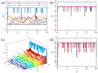
Figure 1: Mean recurrence time for the Heisenberg spin chain. (a) $\langle n\rangle$ for product initial states with four spins sim . (b) The four-spin fractional quantized ensemble mean $\overline{n}$ versus sampling time $\tau$. The mean is $15/8$ except for special values of $\tau$, where it is $14/8$, $13/8$. The blue crosses are numerical simulations (averaging of all states in (a)), and the theoretical red line is given by Eq. (9). (c) $\langle n\rangle$ for six Heisenberg spins. The state $\ket{\uparrow,\downarrow,\downarrow,\downarrow,\downarrow,\downarrow}$ is integer quantized with $\langle n\rangle=6$ for most $\tau$, while for four spins $\langle n\rangle=4$ as shown in (a). (d) The six-spin theoretical (red line) and numerical (blue crosses) $\overline{n}$ perfectly match and exhibit fractional quantization.

Preliminaries. We consider the return problem where the initial state of the monitored spin is up, however, this leaves a plethora of choices for the states of the bath spins. Starting with the Heisenberg model, where $H=\sum_{\langle i,i+1\rangle}\sum_{\alpha=x,y,z}S_{i}^{\alpha}S_{i+1}^{\alpha}$ and $S_{i}^{\alpha}$ are the spin-$\frac{1}{2}$ operators, we plot $\langle n\rangle$ versus the sampling time $\tau$ for a four-spin system in Fig. 1(a). We witness three types of initial conditions. A trivial case is when all bath spins are initially up and then $\langle n\rangle=\sum_{n=1}^{\infty}nF_{n}=1$. This is a stationary state of $H$, and hence recorded with probability one in the first measurement. For other initial states, the average appears a rather intricate function of the sampling time, though in all cases the mean does not exceed $3$, hence the mean detection time is not exceedingly long. Finally, for the initial state $\ket{\uparrow,\downarrow,\downarrow,\downarrow}$, we attain the value $\langle n\rangle=4$ except for resonances, found for special choices of $\tau$. We see that in this case the mean $\langle n\rangle$ is integer quantized, either $1$ for the Zeno limit $\tau\to 0$, or $2$, or $3$, while typically it is $4$. Such an initial state exhibits what we call integer mean recurrence time.

While the sensitivity of the results on the specific initial conditions is clearly seen, when we average evenly over all the initial conditions a remarkably smooth result is found. In Fig. 1(b), the ensemble mean denoted $\overline{n}$, for most $\tau$, is equal to $15/8$. The intricate behaviors of $\langle n\rangle$ are now replaced by a topologically protected behavior encapsulated in the ensemble mean $\overline{n}$. This is a demonstration of the above-mentioned fractional quantum recurrence theorem Bourgain et al. (2014), so that the mean is a fraction, namely $p=15$ and $q=8$ in this case. We also see resonances after averaging, for example transitions where $p$ jumps from $15$ to $14$ and back as we vary the sampling time $\tau$, at the same $\tau$s as found for the initial state $\ket{\uparrow,\downarrow,\downarrow,\downarrow}$. We also show in Fig. 1(c,d) that that the fractional mean for $\overline{n}$ and the integer mean $\langle n\rangle$ for specific initial condition, persists for larger systems. We now study the basics of fractional quantization of $\overline{n}$ in general and later return to the integer mean return time.

Formalism. The measurement of the spin is described by the projection $D^{\uparrow}=\sum_{bath}\ket{\uparrow,bath}\bra{\uparrow,bath}$ and its complement $D_{\downarrow}=1-D^{\uparrow}$. The probability to detect the spin in state up for the first time in the $n$-th measurement is Bourgain et al. (2014)

$$F_{n}=||M_{n}\ket{\psi_{0}}||^{2},\mbox{with}\ \ M_{n}=D^{\uparrow}U(D_{\downarrow}U)^{n-1}.$$ (1)

The operator $M_{n}$ represents the mix of measurements and unitaries $U=\exp(-iH\tau)$, and indicates that $n-1$ measurements failed to detect the spin in the target state, followed by a final success. Analytically $\langle n\rangle$ is found using a generating function technique Bourgain et al. (2014). Let $\hat{M}(e^{i\theta})=\sum_{n=1}^{\infty}M_{n}\exp(in\theta)$, then summing the resulting geometric series

$$\hat{M}(e^{i\theta})=e^{i\theta}D^{\uparrow}U\left(1-e^{i\theta}D_{\downarrow}U\right)^{-1}.$$ (2)

Using the identity $\int_{0}^{2\pi}\exp[i(m-n)\theta]{\rm d}\theta=\delta_{mn}$, we have Bourgain et al. (2014)

$$\langle n\rangle={1\over 2\pi i}\int_{0}^{2\pi}\bra{\psi_{0}}\left[\hat{M}\left(e^{i\theta}\right)\right]^{\dagger}\partial_{\theta}\hat{M}\left(e^{i\theta}\right)\ket{\psi_{0}}{\rm d}\theta.$$ (3)

The mean recurrence time, averaged over the bath states, is

$$\overline{n}={1\over 2^{N-1}}\sum_{b}\int_{0}^{2\pi}\bra{\uparrow,b}\left[\hat{M}\left(e^{i\theta}\right)\right]^{\dagger}\partial_{\theta}\hat{M}\left(e^{i\theta}\right)\ket{\uparrow,b}{{\rm d}\theta\over 2\pi i},$$ (4)

where the $b$ stands for bath. In the denominator, we have $2^{N-1}$ which is the number of states of bath spins. This is our $q$, hence for $N=4$ we have in Fig. 1(b) $q=8$ while in Fig. 1(d) $N=6$ and $q=32$. Eq. (4) contains a bath trace, since we sum matrix elements over all the $2^{N-1}$ bath states. It was shown, in a more general context Bourgain et al. (2014), that this trace can be replaced by

$$\overline{n}={1\over 2^{N-1}}\int_{0}^{2\pi}{\partial_{\theta}{\rm det}\left[\hat{M}\left(e^{i\theta}\right)\right]\over{\rm det}\left[\hat{M}\left(e^{i\theta}\right)\right]}{{\rm d}\theta\over 2\pi i}.$$ (5)

The determinant of $\hat{M}(e^{i\theta})$ is the product of its eigenvalues, some of which are zero. These are set to $\epsilon$, which is then taken to approach 0 with $\partial_{\theta}\epsilon/\epsilon=0$, namely zero eigenvalues are excluded.

$p$ is the number of eigenvalues of the survival operator in the unit disk. To find $p$ we simplify Eq. (5). We use ${\rm det}(ab)={\rm det}(a){\rm det}(b)$ and ${\rm det}(a^{-1})=1/{\rm det}(a)$ and find

$${\rm det}\left[\hat{M}\left(e^{i\theta}\right)\right]={\rm det}[D^{\uparrow}U]{1\over{\rm det}[\exp(-i\theta)-D_{\downarrow}U]}.$$ (6)

The term ${\rm det}[D^{\uparrow}U]$ is $\theta$ independent and using the $\theta$ derivative in Eq. (5) this term is clearly not contributing to $\overline{n}$ not . We now define the survival operator $S=D_{\downarrow}U$ whose eigenvalues are denoted $\xi_{j}$, so ${\rm det}(S-\xi)=0$ and they satisfy $|\xi_{j}|\leq 1$. Using Eqs. (5,6), we can then write

$$\overline{n}={1\over 2q\pi i}\int_{0}^{2\pi}{\partial_{\theta}\ln\left[\Pi_{j=1}^{2^{N}}\left(e^{-i\theta}-\xi_{j}\right)\right]^{-1}{\rm d}\theta}$$ (7)

and $q=2^{N-1}$ as mentioned. Using

$$\int_{0}^{2\pi}{e^{-i\theta}\over e^{-i\theta}-\xi_{j}}{\rm d}\theta=\left\{\begin{array}[]{c c}2\pi&|\xi_{j}|<1\\ 0&|\xi_{j}|=1\end{array}\right.$$ (8)

we find

$$\overline{n}={\mbox{number of}\ \xi_{j}\ \mbox{in the unit disk}\over 2^{N-1}}.$$ (9)

Hence $p$ is the number of eigenvalues of the survival operator $S$ whose absolute values are less than unity. The resonances are found whenever an eigenvalue of $S$ approaches the unit disk as we vary the sampling time $\tau$. Eq. (9) perfectly matches the numerical simulations as shown in Fig. 1, further details in the SM. The number of $\xi$s equal to zero is at least $2^{N-1}$, and hence $1\leq\overline{n}$ which is expected. Since we have in total $2^{N}$ eigenvalues of $S$ for any spin-half model, we find the universal bound

$$1\leq\overline{n}\leq 2.$$ (10)

Such a result is remarkable as the mean number of measurements is less than or equal to 2, independent of the nature of $H$. In some sense, the formula is in the spirit of a speed limit Mandelstam and Tamm (1991); Margolus and Levitin (1998); Sun and Zheng (2019); Van Vu and Saito (2023), though these discuss how two states evolve, while we consider detecting a target state with subspace measurements. The lower bound is reached as an equality for the Ising model on a chain, while the upper bound is found for the Ising model with measurements either in the $X$ or $Y$ direction. Below we will show how the upper bound is approached in the thermodynamic limit for other models.

Dark states give fractional quantization. Eq. (9) is very useful in the evaluation of $\overline{n}$, yet it does not address the main physical aspect of the problem. We claim that $\overline{n}$ provides information on the number of dark states in the system. Dark states $\ket{D}$ are initial conditions that are never detected Thiel et al. (2020); Plenio and Knight (1998). Roughly speaking, under repeated measurements, the Hilbert space is divided into dark and bright subspaces, and it exhibits fragmentation related to ergodicity breaking. We now explain this novel connection between recurrence times and dark states.

Define the eigenvalue problem $S\ket{D}=\xi\ket{D}$. We consider the eigenvalues that are on the unit disk, so $\xi=\exp(-i\gamma)$. It follows that $S^{n-1}\ket{D}=\exp[-i\gamma(n-1)]\ket{D}$. Using Eq. (1) we have $F_{n}=\lVert D^{\uparrow}U\exp[-i\gamma(n-1)]\ket{D}\rVert^{2}$, which is clearly independent of $n$. From the basics of probability, this is possible only if $F_{n}=0$; hence the state $\ket{D}$ is never detected, i.e., dark. It then follows, using $\lVert D^{\uparrow}U\ket{D}\rVert^{2}=0$, that $U\ket{D}=S\ket{D}$, and so $U\ket{D}=\exp(-i\gamma\tau)\ket{D}$. The eigenvalues of $U$ are well-known and given by the exponentials of $-i\tau$ times the energies. We thus conclude that the eigenstates of the survival operator $\ket{D}$, corresponding to eigenvalues on the unit disk $|\xi|=1$, are stationary energy states of the Hamiltonian $H$ with the measured spin in state down. As mentioned, if the initial condition is chosen to be one of these states, the spin is never found in the target state up. Thus the recurrence problem, which deals with bright initial conditions, yields information on the number of dark states in the system and the fragmentation of the Hilbert space. Using Eq. (9) we find

$$\overline{n}=2-{\mbox{number of dark states}\over 2^{N-1}}.$$ (11)

From here we can also infer the resonances. Consider two non-degenerate energy eigenstates, $\ket{E_{1}}$ and $\ket{E_{2}}$, for which the condition $D^{\uparrow}(\alpha_{1}|E_{1}\rangle+\alpha_{2}|E_{2}\rangle)=0$ holds. Then for special $\tau$ matching $\exp(-iE_{1}\tau)=\exp(-iE_{2}\tau)$, the number of dark states will increase by unity, and hence we will experience a resonance in $\overline{n}$, as shown already in Fig. 1. Further examples of dark states that lead to resonances in $\overline{n}$ are discussed in the SM.

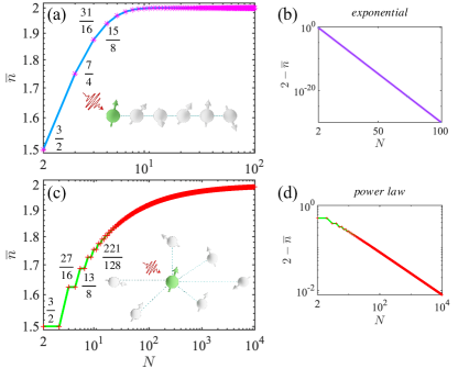
Figure 2: Mean recurrence time as a function of system size $N$. (a) $\overline{n}$ for the Heisenberg spin chain, where the recurrence time exponentially approaches the upper bound in the thermodynamic limit (b). (c) $\overline{n}$ for the XX central spin model, which is fractionally quantized and displays a staircase growth. In (d), we plot $2-\overline{n}$ versus $N$ on a log-log scale, indicating a power-law approach to the upper bound in the thermodynamic limit.

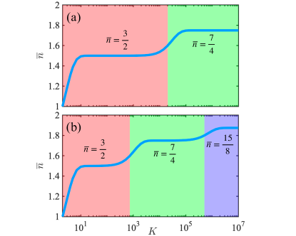
Figure 3: $\overline{n}$ versus the number of measurements reveals fractional staircases. (a) The central three-spin model with $g_{1}=1$ and $g_{2}=0.01$. Two substantial plateaus are visible within $\overline{n}$, which corresponds to an effective two-spin system in small $K$, followed by a transition to the three-spin model for large $K$. (b) The four-spin model. The weakly coupled spins are gradually contributing to $\overline{n}$ as $K$ increases. The figure shows that finite time fractional quantization is valuable for probing local environments.

Scaling of recurrence time with system size. In Fig. 1, the recurrence time is $15/8$ for $N=4$ and $63/32$ for $N=6$, excluding resonances. So how does $\overline{n}$ scale with the system size? Or more fundamentally, how does $\overline{n}$ behave in the thermodynamic limit? To address this, we investigate the behavior of dark states in different models. For the Heisenberg model, our analysis reveals a single dark state, characterized by all spins being down. This state, with an eigenenergy of $(N-1)/4$, leads to $S\ket{D}=\exp[-i(N-1)\tau/4]\ket{D}$. Using Eq. (11), $\overline{n}=2-1/2^{N-1}$ [Fig. 2(a)]. So $\overline{n}$ exponentially approaches the upper bound, see illustration in Fig. 2(b). Distinct behaviors are found for the XX central spin model, where $H=w_{0}S_{0}^{z}+w\sum_{i=1}^{N-1}S_{i}^{z}+\sum_{i=1}^{N-1}g_{i}(S_{0}^{+}S_{i}^{-}+S_{0}^{-}S_{i}^{+})$ Villazon et al. (2020), describing a central spin in a magnetic field $w_{0}$, interacting with bath spins subject to a magnetic field $w$. Here, the condition for the dark states is $\sum_{i=1}^{N-1}g_{i}S_{i}^{-}\ket{D}=0$, and all the dark states are degenerate with eigenenergy $E=-\omega_{0}/2$. As shown in the SM, the number of dark states grows with the size of the system. Using Eq. (11), we have

$$\overline{n}=2-\frac{\Gamma(N)}{\Gamma\left(\lfloor\frac{N+2}{2}\rfloor\right)\Gamma\left(\lfloor\frac{N+1}{2}\rfloor\right)2^{N-1}}.$$ (12)

Here $\Gamma(N)=(N-1)!$ and $\lfloor x\rfloor$ denotes the floor function. As depicted in Fig. 2(c), the mean recurrence time versus $N$ is fractionally quantized and exhibits a unique staircase growth structure. Remarkably, Eq. (12) is valid for any type of coupling $g_{i}$. We next examine the rate at which $\overline{n}$ approaches 2. Using Stirling’s formula, the Gamma function expansion for odd and even $N$ yields $2-\overline{n}\sim\sqrt{2/(\pi N)}$. This indicates a power-law approach towards the upper bound, as shown in Fig. 2(d), contrasting with the exponential behavior observed in Fig. 2(b). The vastly different behaviors are due to the large number of dark states found for the central spin model. A third behavior is found in the Ising model on a ring, where the number of dark states grows exponentially with $N$. Here $\overline{n}=3/2$ is a constant for any $N$, hence the upper bound $\overline{n}\leq 2$ is not saturated in the thermodynamic limit due to the exponential scaling of the number of dark states with system size.

Finite number of measurements. As mentioned, in the thermodynamic limit $\overline{n}$ reaches a constant value. Given a macroscopic system, will we always record this $\overline{n}$ in the $N\rightarrow\infty$ limit, or can we explore various fractional ratios? We claim that the latter is certainly possible, using finite-time experiments. In physical systems, a monitored spin is typically coupled strongly to spins in its vicinity, but weakly to other spins, because the coupling is distance-dependent. We find that using a finite number of measurements, the measured $\overline{n}$ is indifferent to weakly coupled spins. In other words, when the number of measurements is not very large, the system exhibits the behaviors of a small $N$ system. This enables the sensing of different coupling magnitudes and characterizing the distribution of bath spins via $\overline{n}$.

As an illustration, we consider the XXX central spin model (see SM). We assign various $g_{i}$ values and compute the conditional recurrence time $\overline{n}=\sum_{n=1}^{K}nF_{n}/\sum_{n=1}^{K}F_{n}$ for different $K$. $K$ represents the finite number of measurements, controlled in the experiment. In Fig. 3(a), $g_{1}=1$ and $g_{2}=0.01$. When $10^{1}<K<10^{4}$, the weakly coupled spin yields no contribution to $\overline{n}$ and $\overline{n}=3/2$, effectively making it a two-spin system, with a substantial plateau in $\overline{n}$. As $K$ increases, $\overline{n}$ shifts from $3/2$ to $7/4$, where now $\overline{n}$ can “sense” the second weakly coupled bath spin. The color demarcation corresponds to the approximate transition point given by $K=-\log 2/\log(|\xi|)$. We next examine a four-spin system, with $g_{i}=\{1,0.05,0.0025\}$. Depending on the magnitudes of the couplings, $\overline{n}$ senses effectively first one bath spin, then two bath spins, and finally three, as $K$ increases. Consequently, the magnitude of the coupling correlates with the number of measurements required to observe the influence of the weakly coupled spins on $\overline{n}$.

Integer mean return time. The appearance of integer $\langle n\rangle$ is of interest, since it shows when topological effects are present for special initial states. For the Heisenberg model, if we start in state $\ket{\uparrow,\downarrow,\downarrow,\cdots}$ we find $\langle n\rangle=N$ namely, an integer mean recurrence time. The examples of $N=4$, and 6, were presented already in Fig. 1. Thus for this initial state and $N\gg 1$, $\langle n\rangle$ is much larger than the ensemble $\overline{n}$ in Eq. (10). Hence the state with integer quantized $\langle n\rangle$ needs far more measurements to be detected. Interestingly, we find that the integer $\langle n\rangle$ results from the strong correlation between the bath and measured spin. Namely, once the measured spin is recorded in state up, it implies all other spins are down, giving complete knowledge of the bath’s state. This is because the dynamics can be described with an effective single quasi-particle picture: a spinon. We found, with this initial condition, the dynamics are limited to states with single-spin excitations. We have $N$ such states, instead of $2^{N}$ states in general. As mentioned above, the recurrence problem for single-particle is well-studied Grünbaum et al. (2013); Yin et al. (2019). In particular, in single-particle dynamics, we get an integer mean return time, and the integer is the effective dimension of the Hilbert space, which is $N$ for the above-mentioned initial condition but now we recover these properties in the many-body setting.

Conclusion. Employing subspace measurements, we investigated the recurrence time for many-body spin systems under repeated monitoring. The ensemble mean exhibits fractional quantitation, vastly different from the classical case. Intriguingly, a universal bound is derived for the recurrence time, setting both the minimum and maximum speed limits for how quickly a quantum state can complete a cycle and be measured by subspace detection. Remarkably, the fractional recurrence time is determined by the number of dark states in the system. Dark states are a signature of the fragmentation of Hilbert space and ergodicity breaking. Hence by measuring the recurrence time, we can gain insight into an a priori unrelated quantity, the number of dark states in the system. Using dark state physics, we explored how $\overline{n}$ behaves in the limit of large system size, finding four distinct types of behaviors: (1) $\overline{n}$ is $N$ independent as found in the Ising model, $\overline{n}$ is 1 for measurement in the $Z$ direction, while it is 2 for measurement along $X$ and $Y$; (2) $\overline{n}$ exponentially approaches upper bound 2 in the Heisenberg spin model; (3) $\overline{n}$ approaches 2 as a power-law in the central spin model; (4) $\overline{n}$ is 3/2 for the Ising ring model, and hence in this case the upper and lower bounds are not saturated even in the thermodynamic limit. In addition, utilizing the finite number of measurements, which is naturally controlled in experiments, we found that fractional quantization appears as staircases (Fig. 3). This in principle allows one to explore the couplings of a spin to the local environment, with time being a control parameter. Finally, for specific states, we show the complex many-body system can be effectively mapped onto a dynamical system with a single spinon, leading to the presence of integer quantized recurrence times.

The support of Israel Science Foundation’s Grant No. 1614/21 is acknowledged.

Supplemental Material

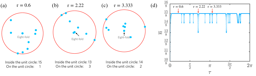
Figure S1: Eigenvalus of the survival operator are distributed on and in the unit disk, fig (a-c), for the four-spin Heisenberg chain. In (d) we show the $\overline{n}$ for the corresponding choices of $\tau$ (see red arrows). (a) For $\tau=0.6$, 15 eigenvalues of the survival operator are located within the unit circle, with one eigenvalue on the unit circle. The ensemble mean recurrence time is determined by the number of eigenvalues within the unit circle divided by $2^{N-1}=8$ since $N=4$. Hence for $\tau=0.6$ we have $\overline{n}=15/8$. (b) At $\tau\simeq 2.22$, $\overline{n}$ decreases to $13/8$, aligning with the number of eigenstates within the unit circle as shown in Figure (b). (c) When $\tau\simeq 3.333$, $\overline{n}$ jumps to $14/8$, and the count of eigenvalues within the unit circle is 14.

Appendix A Recurrence time and eigenvalues of the survival operator

In this section, we present further details on how the $\overline{n}$ is given by the number of eigenvalues of the survival operator. In the Letter, the theoretical Eq. (9) gives a perfect match with the numerical $\overline{n}$, as shown in Figs. 1(b,d). In Fig. S1, we plot the exact distribution of the eigenvalues of the survival operator for specific sampling times $\tau$. This offers a more visible presentation of how the recurrence time is connected to the eigenvalues $\xi$. Specifically, we plot the eigenvalues $\xi$s for different values of $\tau$ for the four-spin Heisenberg spin chain. This model was defined in the preliminary in the Letter. When $\tau=0.6$, there are 15 $\xi$s inside the unit disk. Using Eq. (9), we find $\overline{n}=15/8$, consistent with the numerical simulation in Fig. S1 (d). In fact, for any $\tau$ where $\overline{n}=15/8$, 15 $\xi$s are found inside the unit circle. When $\tau\simeq 2.22$, the $\overline{n}$ jumps to $13/8$. Now, the number of $\xi$ inside the unit circle is 13, as shown in Fig. S1 (b). Similarly, for $\tau\simeq 3.333$, there are 14 $\xi$s inside the unit circle and $\overline{n}=7/4$.

Appendix B Dark states and resonances

We have seen resonances in the ensemble mean recurrence time, for examples in Fig. 1 and Fig. S1, which give rise to point-wise discontinuities in $\overline{n}$. In the Letter, we show that this is because of the additional dark states, which appear when the condition $D^{\uparrow}(\alpha_{1}|E_{1}\rangle+\alpha_{2}|E_{2}\rangle)=0$ is fulfilled, where $E_{1}\neq E_{2}$. In this section, we present the detailed steps for the construction of additional dark states for the central spin model.

We first discuss the general properties of the central spin model Villazon et al. (2020). As mentioned in the Letter, the Hamiltonian of the XX central spin model is

$$H=w_{0}S_{0}^{z}+w\sum_{i=1}^{N-1}S_{i}^{z}+\sum_{i=1}^{N-1}g_{i}(S_{0}^{+}S_{i}^{-}+S_{0}^{-}S_{i}^{+}),$$ (S1)

where $S_{i}^{\pm}=S_{i}^{x}\pm iS_{i}^{y}$. The spectrum of this model is solved in Villazon et al. (2020). The eigenstates of $H$ are divided into four groups: $|D^{+}\rangle,|{\cal B}(E)\rangle,|{\cal B}(-E)\rangle$, and $|D\rangle$. We soon show why we denote these symbols. The central spin Hamiltonian is diagonalized by these states. The eigenfunction for the states $|{\cal B}(E)\rangle$ and $|{\cal B}(-E)\rangle$ are

$$H|{\cal B}(E)\rangle=E|{\cal B}(E)\rangle,\quad H|{\cal B}(-E)\rangle=-E|{\cal B}(-E)\rangle$$ (S2)

Using the Bethe ansatz, in the subspace with $K$ spin excitations atop the vacuum $|0\rangle$ (all the spins are in the state down), we have Villazon et al. (2020)

$$|{\cal B}(E)\rangle$$ (S3)

$$=\left[G^{+}(0)+\left(E+\frac{\omega_{0}}{2}\right)S_{0}^{+}\right]G^{+}(v_{1})\cdots G^{+}(v_{K-1})|0\rangle,$$

$$|{\cal B}(-E)\rangle$$

$$=\left[G^{+}(0)+\left(-E+\frac{\omega_{0}}{2}\right)S_{0}^{+}\right]G^{+}(v_{1})\cdots G^{+}(v_{K-1})|0\rangle,$$

where $G^{+}(v)=\sum_{i=1}^{N-1}g_{i}/(1-g_{i}^{2}v)S_{i}^{+}$. The parameters $v_{i}$ are given by:

$$1+v_{a}\sum_{i=1}^{N-1}\frac{g_{i}^{2}}{2(1-g_{i}^{2}v_{a})}-v_{a}\sum_{b\neq a}^{K-1}\frac{1}{v_{b}-v_{a}}=0,$$ (S4)

for $a=1\ldots K-1$. The eigenenergy is given by Villazon et al. (2020)

$$E^{2}=\frac{\omega_{0}^{2}}{4}+\left(\sum_{i=1}^{N-1}g_{i}^{2}-\sum_{i=1}^{K-1}\frac{2}{v_{i}}\right).$$ (S5)

Each solution for $v_{1}\ldots v_{N-1}$ leads to two possible solutions for $E$, exhibiting level repulsion.

For the states $|D\rangle$, we have $H|D\rangle=-w_{0}/2|D\rangle$, which are the dark states we have discussed in the main text. The states $|D^{+}\rangle$ have the same bath states as $|D\rangle$ but with the monitored spin in the up state, hence its eigenenergy is $w_{0}/2$ The resonances are given by the states $|{\cal B}(E)\rangle,|{\cal B}(-E)\rangle$ fits the condition we found, hence we now only focus on the states $|{\cal B}(E)\rangle,|{\cal B}(-E)\rangle$. Using Eq. (S3), we rewrite the states $|{\cal B}(E)\rangle,|{\cal B}(-E)\rangle$ as:

$$|{\cal B}(E)\rangle={\cal N}\left[\mid\downarrow\rangle_{0}\otimes|\beta^{\downarrow}\rangle+\left(E+\frac{\omega_{0}}{2}\right)\mid\uparrow\rangle_{0}\otimes|\beta^{\uparrow}\rangle\right],$$ (S6)

$$|{\cal B}(-E)\rangle={\cal N}\left[\mid\downarrow\rangle_{0}\otimes|\beta^{\downarrow}\rangle+\left(-E+\frac{\omega_{0}}{2}\right)\mid\uparrow\rangle_{0}\otimes|\beta^{\uparrow}\rangle\right],$$

where the states $|\beta^{\downarrow}\rangle=G^{+}(0)G^{+}(v_{1})\cdots G^{+}(v_{K-1})|0\rangle$ and $|\beta^{\uparrow}\rangle=G^{+}(v_{1})\cdots G^{+}(v_{K-1})|0\rangle$ denote the states of the bath spins and ${\cal N}$ is for the normalization.

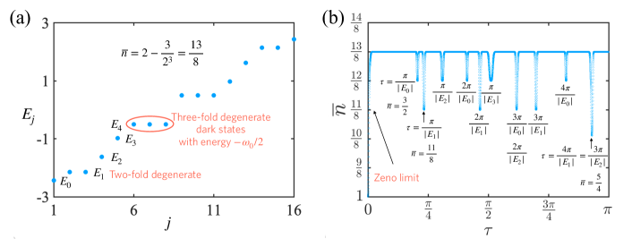
Figure S2: Additional dark states lead to the resonances in $\overline{n}$ for special sampling times. Here $g_{1}=1.221$, $g_{2}=0.864$, and $g_{3}=1.46$, though the main physical effects are not sensitive to these couplings. (a) The energy spectrum of the system. The three states corresponding to the degenerate energy level $E_{4}=-w_{0}/2=-1/2$ are typical dark states. The mean recurrence time is determined by the three dark states, hence $\overline{n}=2-3/8=13/8$, aligning with the numerical simulations in (b) except the resonances. (b) The plot of $\overline{n}$ versus the sampling time $\tau$. When the number of dark states changes, due to the appearance of additional dark states, found for special $\tau$, $\overline{n}$ exhibits the resonances. The energy levels in (a) can be used to understand the locations of dips, namely the special sampling times, as presented in (b).

We now explain the resonances in the recurrence time. Apart from the dark states that are directly derived from the Hamiltonian’s eigenstates ($|D\rangle$), we introduce another category of dark state, which is associated with the sampling time $\tau$ and leads to the resonances in $\overline{n}$, for examples in Fig. 1. In the central spin model, the interrelation between the eigenstates with energy $E$ and $-E$ [see Eq.(S6)] allows for the construction of the additional dark states. The condition $D^{\uparrow}(\alpha_{1}|E_{1}\rangle+\alpha_{2}|E_{2}\rangle)=0$ in the Letter leads to

$$\Delta E\tau=2k\pi,\quad k\quad\text{is an integer.}$$ (S7)

Namely $\Delta E\tau=2E\tau$ for the central spin model. Using Eq. (S6), we find that $U|{\cal B}(E)\rangle=\exp(-ik\pi)|{\cal B}(E)\rangle$ and $U|{\cal B}(-E)\rangle=\exp(ik\pi)|{\cal B}(-E)\rangle$, where $\exp(-ik\pi)=\exp(ik\pi)$. Consequently, the states $|{\cal B}(E)\rangle$ and $|{\cal B}(-E)\rangle$ act as degenerate states under the unitary action $U$. We denote the linear combination of these two states as $|D^{S}\rangle$, such that

$$|D^{S}\rangle=c_{1}|{\cal B}(E)\rangle+c_{2}|{\cal B}(-E)\rangle=\mid\downarrow\rangle_{0}\otimes|\beta^{\downarrow}\rangle.$$ (S8)

Using Eq. (S6), we have $c_{1}=(2E-w_{0})\sqrt{\langle\beta^{\downarrow}|\beta^{\downarrow}\rangle+(E+w_{0}/2)^{2}\langle\beta^{\uparrow}|\beta^{\uparrow}\rangle}/(4E)$ and $c_{2}=(2E+w_{0})\sqrt{\langle\beta^{\downarrow}|\beta^{\downarrow}\rangle+(w_{0}/2-E)^{2}\langle\beta^{\uparrow}|\beta^{\uparrow}\rangle}/(4E)$. For the constructed state $|D^{S}\rangle$, when the sampling time satisfies the condition in Eq. (S7), we obtain

$$S|D^{S}\rangle=e^{-ik\pi}|D^{S}\rangle=e^{ik\pi}|D^{S}\rangle.$$ (S9)

Here, $|D^{S}\rangle$ is an eigenstate of the survival operator with an eigenvalue $|\xi|=|\exp(-ik\pi)|=1$. Consequently, $|D^{S}\rangle$ also qualifies as a dark state. When $\tau\neq k\pi/E$, we find that $S|D^{S}\rangle=D_{\downarrow}[c_{1}\exp(-iE\tau)|{\cal B}(E)\rangle+c_{2}\exp(iE\tau)|{\cal B}(-E)\rangle]$. Therefore, the state $|D^{S}\rangle$ is not an eigenstate of $S$ under these conditions. In other words, $|D^{S}\rangle$ only emerges for specific sampling times given in Eq. (S7). Using Eq. (11), we can infer that the recurrence time will exhibit a sharp jump when these dark states appear.

The above discussion is generic for any central spin models. As an example, we confirm Eqs. (S7-S9) with the four-spin case. As shown in Fig. S2, we have ten distinct energy levels, five with $E<0$ and five with $E>0$. We label energy levels as $E_{0}<E_{1}<E_{2}<E_{3}<0$. The states corresponding to $E_{4}$ are typical dark states as we discussed in the Letter, i.e., independent of sampling time $\tau$. As there are three typical dark states, we have $\overline{n}=13/8$, which is confirmed with numerical simulations as shown in Fig. S2(b) for most of $\tau$s except the resonances. For the resonances, when $\tau$ increases, energy levels begin to satisfy the condition in Eq. (S7). The energy level $E_{0}$ possesses the largest absolute value, and when $\tau=\pi/|E_{0}|$, a new dark state is constructed using Eq. (S8). Consequently, instead of three dark states we now have four dark states in total and $\overline{n}=2-4/8=3/2$, which is in agreement with the results in Fig. S2(b). When $\tau=\pi/|E_{1}|$, two additional dark states are constructed with Eq. (S8) due to the two-fold degeneracy of the energy level $E_{1}$, leading to $\overline{n}=11/8$. In a similar fashion, all the jumps in the recurrence time can be explained using the rise of the dark states. A special case occurs when $\tau=4\pi/|E_{1}|=3\pi/|E_{2}|$, where energy levels $E_{1}$ and $E_{2}$ simultaneously satisfy Eq. (S7). In this case, three additional dark states are constructed, resulting in $\overline{n}=5/4$.

Appendix C Counting the number of dark states

In this section, we study the number of dark states for the central spin model Eq. (S1). We derive Eq. (12) in the main text.

No excitations. We start with the ground state, denoted $|\psi\rangle_{0}=\mid\downarrow,\downarrow,\cdots\rangle$. Here all the spins are in the down state, i.e., the vacuum state. The subscript $0$ in $|\psi\rangle_{0}$ denotes zero spin excitations. It is easy to check that this is an eigenstate of $H$. This is because $\sum_{i=1}^{N-1}g_{i}S_{0}^{+}S_{i}^{-}|\psi\rangle_{0}=0$ and $S_{0}^{-}|\psi\rangle_{0}=0$. We have a unique disentangled state when the number of spin excitations in the sector is zero. By sector, we mean that here we study only the cases where the central spin is in the down state. The energy of the state $|\psi\rangle_{0}$ is $-\omega_{0}/2$. Clearly, this state, being an eigenstate of $H$, is a dark state, as any click will detect the central spin in the state down.

One excitation states. We now find disentangled dark states with a single excitation of the bath states, denoted $|\psi\rangle_{1}$ where the subscript is for the number of excitations. For example, consider the case of four bath spins. We will find an eigenstate of $H$ such that

$$|\psi\rangle_{1}= \alpha_{1}\mid\downarrow,\uparrow,\downarrow,\downarrow,\downarrow\rangle+\alpha_{2}\mid\downarrow,\downarrow,\uparrow,\downarrow,\downarrow\rangle+$$ (S10)

$$\alpha_{3}\mid\downarrow,\downarrow,\downarrow,\uparrow,\downarrow\rangle+\alpha_{4}\mid\downarrow,\downarrow,\downarrow,\downarrow,\uparrow\rangle.$$

Again, since this is a stationary state and since the central spin is in state down, this state will remain forever dark, and the string of measurements will be down, down, down, till infinity. The condition that this holds is, as before, $\sum_{i=1}^{N-1}g_{i}S_{0}^{+}S_{i}^{-}|\psi\rangle_{1}=0$. Define two vectors, the first composed of the unknowns $\vec{\alpha}=(\alpha_{1},\cdots,\alpha_{N-1})$ and the second from the prescribed couplings $\vec{g}=(g_{1},\cdots,g_{N-1})$. Then we clearly need to solve $\vec{\alpha}\cdot\vec{g}=0$. Since $\vec{g}$ is a vector of length $N-1$ given by the coupling constants, we know from basic geometry, that we have $N-2$ vectors orthogonal to $\vec{g}$, which are also mutually orthogonal. As usual, they can be also normalized but this is of little concern here. We reject the trivial solution $\vec{\alpha}=0$ since it does not represent a state. The important conclusion for us is that we have $N-2$ dark states with a single bath excitation. We remark that the energy of this state is again, $-\omega_{0}/2$, and the same holds for all the dark states considered below. The central spin and bath spins are not entangled because in general the dark state is $|D\rangle=\mid\downarrow\rangle\otimes|\psi\rangle_{i}$, which is separable.

Two spin excitations. We now consider dark states $|\psi\rangle_{2}$ with two spin excitations, for example for four bath spins we have

$$|\psi\rangle_{2}= \alpha_{12}\mid\downarrow,\uparrow,\uparrow,\downarrow,\downarrow\rangle+\alpha_{13}\mid\downarrow,\uparrow,\downarrow,\uparrow,\downarrow\rangle+\alpha_{14}\mid\downarrow,\uparrow,\downarrow,\downarrow,\uparrow\rangle+$$ (S11)

$$\alpha_{23}\mid\downarrow,\downarrow,\uparrow,\uparrow,\downarrow\rangle+\alpha_{24}\mid\downarrow,\downarrow,\uparrow,\downarrow,\uparrow\rangle+\alpha_{34}\mid\downarrow,\downarrow,\downarrow,\uparrow,\uparrow\rangle.$$

Like before the central spin is in state down, so this is a dark state. The matrix element, $\alpha_{ij}$ indicates that the $i$-th and the $j$-th bath spins are excited, so these indexes run from $1$ to $N-1$. Clearly, the diagonal elements $\alpha_{ii}$ are zero, and $\alpha_{ij}=\alpha_{ji}$. In this example, with $4$ spins in the bath, we have six unknowns, $\alpha_{12},\alpha_{13},\alpha_{14},\alpha_{23},\alpha_{24}$ and $\alpha_{34}$. As before these states are dark eigen states of $H$ if $\sum_{i=1}^{N-1}g_{i}S_{0}^{+}S_{i}^{-}|\psi\rangle_{2}=0$. This means that for four bath spins we must solve

$$\left(\begin{array}[]{c c c c}0&\alpha_{12}&\alpha_{13}&\alpha_{14}\\ \alpha_{12}&0&\alpha_{23}&\alpha_{24}\\ \alpha_{13}&\alpha_{23}&0&\alpha_{34}\\ \alpha_{14}&\alpha_{24}&\alpha_{34}&0\end{array}\right)\left(\begin{array}[]{c}g_{1}\\ g_{2}\\ g_{3}\\ g_{4}\end{array}\right)=0.$$ (S12)

Clearly in this example we have $4$ equations and $6$ unknowns and hence we find two independent solutions. Technically, we may choose two coefficients as seeds, for example $\alpha_{34},\alpha_{24}$. If these are set to zero, a short calculation shows that the other $\alpha_{ij}$ must be zero as well, however this does not describe a legitimate state. Hence we have two solutions that can be easily found assigning say $\alpha_{34}=1,\alpha_{24}=0$ and vice versa. Other pairs of seeds can be assigned, and then with simple linear algebra, namely using the Gram-Schmidt orthoganalization, we find the constants $\alpha_{ij}$ and the orthogonal states. Again, this is not our aim here, our focus is that for $N=5$ we have two dark states. More generally, the number of dark states is the number of matrix elements above (or below) the diagonal of an $N-1\times N-1$ matrix, minus the number of constraints namely the dimension of the vector $\vec{g}$ which is $N-1$. Hence

number of dark states with a pair of excitations =

$$\left(\begin{array}[]{c}N-1\\ 2\end{array}\right)-\left(\begin{array}[]{c}N-1\\ 1\end{array}\right)={(N-4)(N-1)\over 2}.$$ (S17)

Here we assumed that $N>4$ otherwise the number of dark states with two excitations is zero.

Eq. (S17) has a simple combinatorial meaning. For two spin excitations, among $N-1$ bath spins, we have $\left(\begin{array}[]{c}N-1\\ 2\end{array}\right)$ ways to arrange the spins. This is the number of $\alpha_{ij}$s one needs to determine. On the other hand the operation of $\sum_{i=1}^{N-1}g_{i}S_{0}^{+}S_{i}^{-}$ on the two spin excitation states $|\psi\rangle_{2}$ is clearly to take the central spin denoted with $0$ from the down state to up, while annihilating one of the two excitations. This means that for the bath spins we are left with one spin in state up. The number of such states is clearly $\left(\begin{array}[]{c}N-1\\ 1\end{array}\right)$. This is the reason why Eq. (S17) holds. To see this, note that $\sum_{i=1}^{N-1}g_{i}S_{0}^{+}S_{i}^{-}|\psi\rangle_{2}=0$ gives a linear combination of states with a single spin bath excitation, however these are all orthogonal, so multiplying by kets composed of these $N-1$ single bath spin excitation vectors, will give $N-1$ equations to determine the unknowns $\alpha_{ij}$. This leaves $\left(\begin{array}[]{c}N-1\\ 2\end{array}\right)-\left(\begin{array}[]{c}N-1\\ 1\end{array}\right)$ floating $\alpha_{ij}$s. Let us denote this number by $N_{2D}$. We choose $N_{2D}$ members of the set $\alpha_{ij}$. We assign to these floating $\alpha_{ij}$s orthogonal vectors [like what we did for $(\alpha_{34},\alpha_{24})\rightarrow(1,0)$ and $(0,1)$], but now we have $N_{2D}$ such vectors instead of two]. From these seed vectors we find in principle the other $\alpha_{ij}$. Hence $N_{2D}$ is also the number of dark states for two bath spin excitations.

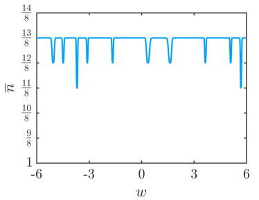
Figure S3: The ensemble mean $\overline{n}$ versus the magnitude of magnetic fields. Here we use the central spin model given in Eq. (S1) and $g_{1}=1.221$, $g_{2}=0.864$, and $g_{3}=1.46$. The sampling time $\tau=1$ is a constant.

Three excited spins. The number of ways to arrange $2$ spins among $N-1$ is $\left(\begin{array}[]{c}N-1\\ 2\end{array}\right)$, this being the number of equations for the $\alpha_{ijk}$ to be solved. The number of unknowns (number of possible three spin excitations) is $\left(\begin{array}[]{c}N-1\\ 3\end{array}\right)$. Hence

number of dark states with three excitations =

$$\left(\begin{array}[]{c}N-1\\ 3\end{array}\right)-\left(\begin{array}[]{c}N-1\\ 2\end{array}\right).$$ (S22)

For $N=5$ we get a negative number, so there are no dark states in this case. A similar cutoff will be found in general for other values of $N$.

$K$ excited spins. In general, we see that for a bath with $K$ excited spins, hence clearly $K\leq N$, we have

number of dark states with $$K$$ excitations =

$$\left(\begin{array}[]{c}N-1\\ K\end{array}\right)-\left(\begin{array}[]{c}N-1\\ K-1\end{array}\right).$$ (S27)

Clearly the number of dark states cannot be negative. Thus the maximum $K$, beyond which we cannot find dark states, is easily shown to be $K_{{\rm max}}=N/2$ if $N$ is even, or $K_{{\rm max}}=(N-1)/2$ if $N$ is odd. This result can also be derived using the Beta Anzats treatment PhysRevLett.91.246802; Villazon et al. (2020). We now find the total number of dark states summing over the number of dark states for the different values of excited spins in the bath

$$\underbrace{\left(\begin{array}[]{c}N-1\\ 0\end{array}\right)}_{0\ \mbox{excitations}}+\underbrace{\left(\begin{array}[]{c}N-1\\ 1\end{array}\right)-\left(\begin{array}[]{c}N-1\\ 0\end{array}\right)}_{1\ \mbox{excitations}}+$$ (S34)

$$\underbrace{\left(\begin{array}[]{c}N-1\\ 2\end{array}\right)-\left(\begin{array}[]{c}N-1\\ 1\end{array}\right)}_{2\ \mbox{excitations}}+\cdots\underbrace{\left(\begin{array}[]{c}N-1\\ K_{{\rm max}}\end{array}\right)-\left(\begin{array}[]{c}N-1\\ K_{{\rm max}}-1\end{array}\right)}_{K_{{\rm max}}\ \mbox{excitations}}$$ (S43)

Hence we conclude

$$\mbox{total number of dark states =}\ \ \frac{\Gamma(N)}{\Gamma\left(\lfloor\frac{N+2}{2}\rfloor\right)\Gamma\left(\lfloor\frac{N+1}{2}\rfloor\right)2}.$$ (S44)

Together with Eq. (11), we get the mean recurrence time versus $N$ for the central spin model as shown in Eq. (12). Note that this equation is not valid at resonances as previously discussed.

We noted already that the energy of all the dark states is $-\omega_{0}/2$ if $\omega=0$. If $\omega\neq 0$ in Eq. (S1) the degeneracy of these states would be partially removed, though states with $K$ excitations will have the same energy. However, the eigenfunctions would remain unchanged, hence also when $\omega\neq 0$, the number of dark states is given in Eq. (S44). This in turn implies that a magnetic field $\omega$ will not modify the fractional mean return time, even if the degeneracy is lifted, see Fig. S3.

Appendix D XXX central spin model

In the finite number of measurements section, we utilize the XXX central spin model. The Hamiltonian of the XXX central spin model is given by:

$$H=w_{0}S_{0}^{z}+w\sum_{i=1}^{N-1}S_{i}^{z}+\sum_{i=1}^{N-1}g_{i}(S_{0}^{x}S_{i}^{x}+S_{0}^{y}S_{i}^{y}+S_{0}^{z}S_{i}^{z}).$$ (S45)

Here, the central spin $S_{0}$ is subject to an external magnetic field $w_{0}$, and the bath spins are subject to a magnetic field of strength $w$. This model differs from the XX central spin model defined in the Letter, as the coupling between the central spin and bath spins occurs in the $X$, $Y$, and $Z$ directions.

The model is classified into isotropic or anisotropic cases, depending on whether the coupling constant $g_{i}$ is uniform (for instance, $g_{i}=\text{constant}$, with all $g_{i}$ equal to one) or varied (e.g., $g_{i}=1$, $g_{2}=1.5$, etc.). For the isotropic XXX central spin model, the ensemble mean recurrence time as a function of system size is the same as that in the XX central spin model discussed in the Letter. However, it should be noted that for the XX central spin model, Eq. (12) is valid regardless of whether $g_{i}$ values are identical or varied.

For the anisotropic XXX central spin model, the ensemble mean recurrence time as a function of system size is expressed as:

$$\overline{n}=2-\frac{1}{2^{N-1}}.$$ (S46)

This equation mirrors the scaling behavior observed in the Heisenberg spin chain. Furthermore, these results suggest that the typical behaviors we presented in the Letter are representative and applicable to other models.

References

- Redner (2001) S. Redner, A Guide to First-Passage Processes (Cambridge University Press, Cambridge, England, 2001).
- Metzler et al. (2014) R. Metzler, G. Oshanin, and S. Redner, First-Passage Phenomena and Their Applications (World Scientific, Singapore, 2014).
- Bray et al. (2013) A. J. Bray, S. N. Majumdar, and G. Schehr, Adv. Phys. 62, 225 (2013).
- Bénichou and Voituriez (2014) O. Bénichou and R. Voituriez, Phys. Rep. 539, 225 (2014).
- Guérin et al. (2016) T. Guérin, N. Levernier, O. Bénichou, and R. Voituriez, Nature 534, 356 (2016).
- Bebon and Godec (2023) R. Bebon and A. Godec, Phys. Rev. Lett. 131, 237101 (2023).
- Krovi and Brun (2007) H. Krovi and T. A. Brun, Phys. Rev. A 75, 062332 (2007).
- Dhar et al. (2015a) S. Dhar, S. Dasgupta, A. Dhar, and D. Sen, Phys. Rev. A 91, 062115 (2015a).
- Dhar et al. (2015b) S. Dhar, S. Dasgupta, and A. Dhar, J. Phys. A: Math. Theor. 48, 115304 (2015b).
- Friedman et al. (2017) H. Friedman, D. A. Kessler, and E. Barkai, Phys. Rev. E 95, 032141 (2017).
- Pöpperl et al. (2023) P. Pöpperl, I. V. Gornyi, and Y. Gefen, Phys. Rev. B 107, 174203 (2023).
- (12) M. Kulkarni and S. N. Majumdar, arXiv:2305.15123 .
- Krapivsky et al. (2014) P. L. Krapivsky, J. M. Luck, and K. Mallick, J. Stat. Phys. 154, 1430 (2014).
- Lahiri and Dhar (2019) S. Lahiri and A. Dhar, Phys. Rev. A 99, 012101 (2019).
- Thiel et al. (2018) F. Thiel, E. Barkai, and D. A. Kessler, Phys. Rev. Lett. 120, 040502 (2018).
- Yin et al. (2019) R. Yin, K. Ziegler, F. Thiel, and E. Barkai, Phys. Rev. Res. 1, 033086 (2019).
- Das and Gupta (2022) D. Das and S. Gupta, J. Stat. Mech. 2022, 033212 (2022).
- Das et al. (2022) D. Das, S. Dattagupta, and S. Gupta, J. Stat. Mech. 2022, 053101 (2022).
- Wang et al. (2023) Y.-J. Wang, R.-Y. Yin, L.-Y. Dou, A.-N. Zhang, and X.-B. Song, Phys. Rev. Res. 5, 013202 (2023).
- Kulkarni and Majumdar (2023) M. Kulkarni and S. N. Majumdar, J. Phys. A: Math. Theor. 56, 385003 (2023).
- Acharya and Gupta (2023) A. Acharya and S. Gupta, Phys. Rev. E 108, 064125 (2023).
- Dubey et al. (2021) V. Dubey, C. Bernardin, and A. Dhar, Phys. Rev. A 103, 032221 (2021).
- Thiel et al. (2020) F. Thiel, I. Mualem, D. Meidan, E. Barkai, and D. A. Kessler, Phys. Rev. Res. 2, 043107 (2020).
- Yin and Barkai (2023) R. Yin and E. Barkai, Phys. Rev. Lett. 130, 050802 (2023).
- Dhar and Dasgupta (2016) S. Dhar and S. Dasgupta, Phys. Rev. A 93, 050103 (2016).
- Krapivsky et al. (2018) P. L. Krapivsky, J. M. Luck, and K. Mallick, J. Stat. Mech. 2018, 023104 (2018).
- Agranov and Meerson (2018) T. Agranov and B. Meerson, Phys. Rev. Lett. 120, 120601 (2018).
- Ro et al. (2023) S. Ro, J. Yi, and Y. W. Kim, Phys. Rev. E 107, 064143 (2023).
- Dittel et al. (2023) C. Dittel, N. Neubrand, F. Thiel, and A. Buchleitner, Phys. Rev. A 107, 052206 (2023).
- (30) B. Walter, G. Perfetto, and A. Gambassi, arXiv:2311.05585 .
- (31) A. Purkayastha and A. Imparato, arXiv:2306.01586 .
- (32) J. B. Hass, I. Corwin, and E. I. Corwin, arXiv:2308.01267 .
- Boltzmann (1896) L. Boltzmann, Vorlesungen über Gastheorie (J.A. Barth, Leipzig, 1896).
- Grünbaum et al. (2013) F. A. Grünbaum, L. Velázquez, A. H. Werner, and R. F. Werner, Commun. Math. Phys. 320, 543 (2013).
- Bourgain et al. (2014) J. Bourgain, F. A. Grünbaum, L. Velázquez, and J. Wilkening, Commun. Math. Phys. 329, 1031 (2014).
- Aharonov and Anandan (1987) Y. Aharonov and J. Anandan, Phys. Rev. Lett. 58, 1593 (1987).
- Tornow and Ziegler (2023) S. Tornow and K. Ziegler, Phys. Rev. Res. 5, 033089 (2023).
- Cech et al. (2023) M. Cech, I. Lesanovsky, and F. Carollo, Phys. Rev. Lett. 131, 120401 (2023).
- (39) In the numerical and , the resonances are with finite width. This is because the number of measurements in the numerical simulations is finite. If we extend the sum over to infinity, the width will disappear and the resonances are point-wise discontinuities.
- (40) Actually, is zero, hence as mentioned under Eq. (5) the epsilon regularization is implied.
- Mandelstam and Tamm (1991) L. Mandelstam and I. Tamm, in Selected Papers (Springer, Berlin, Heidelberg, 1991) pp. 115–123.
- Margolus and Levitin (1998) N. Margolus and L. B. Levitin, Physica D 120, 188 (1998).
- Sun and Zheng (2019) S. Sun and Y. Zheng, Phys. Rev. Lett. 123, 180403 (2019).
- Van Vu and Saito (2023) T. Van Vu and K. Saito, Phys. Rev. Lett. 130, 010402 (2023).
- Plenio and Knight (1998) M. B. Plenio and P. L. Knight, Rev. Mod. Phys. 70, 101 (1998).
- Villazon et al. (2020) T. Villazon, A. Chandran, and P. W. Claeys, Phys. Rev. Res. 2, 032052 (2020).