Top-$K$ ranking with a monotone adversary

Abstract

In this paper, we address the top-$K$ ranking problem with a monotone adversary. We consider the scenario where a comparison graph is randomly generated and the adversary is allowed to add arbitrary edges. The statistician’s goal is then to accurately identify the top-$K$ preferred items based on pairwise comparisons derived from this semi-random comparison graph. The main contribution of this paper is to develop a weighted maximum likelihood estimator (MLE) that achieves near-optimal sample complexity, up to a $\log^{2}(n)$ factor, where $n$ denotes the number of items under comparison. This is made possible through a combination of analytical and algorithmic innovations. On the analytical front, we provide a refined $\ell_{\infty}$ error analysis of the weighted MLE that is more explicit and tighter than existing analyses. It relates the $\ell_{\infty}$ error with the spectral properties of the weighted comparison graph. Motivated by this, our algorithmic innovation involves the development of an SDP-based approach to reweight the semi-random graph and meet specified spectral properties. Additionally, we propose a first-order method based on the Matrix Multiplicative Weight Update (MMWU) framework. This method efficiently solves the resulting SDP in nearly-linear time relative to the size of the semi-random comparison graph.

1 Introduction

In this paper we consider the problem of ranking $n$ items given pairwise comparisons among them. This problem finds numerous applications in recommendation system [WYH⁺18], rating players [Elo67], web search [DKNS01], etc. One widely adopted model for pairwise comparison data is the Bradley-Terry-Luce (BTL) model [BT52, Luc05]. In this model, one assumes a latent score vector $\bm{\theta}^{\star}\in\mathbb{R}^{n}$, and that the Bernoulli outcome of the comparison between items $i$ and $j$ follows

$$\mathbb{P}\left[\text{\text{ item $i$ is preferred over item $j$ }}\right]=\frac{e^{\theta_{i}^{\star}}}{e^{\theta_{i}^{\star}}+e^{\theta_{j}^{\star}}}.$$

It is intuitive that under the BTL model, a higher score indicates a higher chance of winning a comparison.

In practice, the comparisons are often made for a subset of all possible pairs. A popular model to accommodate this situation is the uniform sampling model [CS15, CFMW19], i.e., each pair is compared independently with probability $p$. Uniform sampling is quite convenient for theory. An an example, under this sampling mechanism, [CFMW19] shows that with high probability, the (regularized) maximum likelihood estimator (MLE) [FJ57] exactly identifies the top $K$ preferred items with an optimal sample complexity:

$$n^{2}p\gtrsim\frac{n\log(n)}{\Delta_{K}^{2}},$$ (1)

where $\Delta_{K}$ measures the latent score difference between the $K$-th and the $(K+1)$-th preferred items, and $n^{2}p$ is the expected number of comparisons.

Uniform sampling, while convenient for theoretical purposes, is often too ideal to match practice. This motivates a line of work [SBB⁺16, LSR22, Che23] that goes beyond uniform sampling and focuses on general sampling mechanisms. However, the theoretical guarantees are far from satisfactory. Take the recent work [LSR22] on the general sampling case as an example. The (regularized) MLE requires a sample complexity of $n^{2}p\gtrsim\Delta_{K}^{-2}p^{-1}n\log(n)$ when applied to the special case of uniform sampling. For a sparse random graph, i.e., when $p\gtrsim\log(n)/n$, this sample complexity could be $n$ times larger than the optimal one (1).

In this paper we aim to find a middle ground between uniform and general sampling mechanisms. Inspired by a line of work [BS95, FK01, MMV12, MPW16, AV18, CG18, KLL⁺23, GC23], we consider the so-called semi-random sampling where some benign adversary is allowed to make more comparisons in addition to uniform sampling; see Figure 2. Given its monotone nature, this is sometimes also referred to as a monotone adversary. Intuitively, the monotone adversary should bring no harm to the ranking problem as it only reveals more information about the underlying score vector $\bm{\theta}^{\star}$. However, it is well documented in the literature that the monotone adversary poses serious algorithmic and analytical challenges for a variety of problems. In community detection, [MPW16] shows that the information-theoretic detection limit could shift given a monotone adversary. In problems including sparse recovery [KLL⁺23] and matrix completion [CG18], methods and analyses that work well for uniform sampling can fail dramatically with a semi-random adversary. In this paper, we investigate top-$K$ ranking under semi-random sampling. Our goal is to address the following question:

Can we identify the top-$K$ items with minimal sample complexity, even under a monotone adversary?

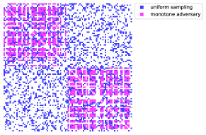
Figure 1: Adjacency matrix of a semi-random comparison graph. Each non-white square corresponds to a non-zero entry in the adjacency matrix.

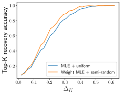
Figure 2: Accuracy of top-$K$ recovery for MLE under uniform sampling and weighted MLE under semi-random sampling. See Section F for the experiment setup.

1.1 Technical challenges

Top-$K$ ranking under semi-random sampling brings some unique challenges. To begin with, it is worth noting that bounding the $\ell_{2}$ estimation error for the score vector $\bm{\theta}^{\star}$ is not sufficient to guarantee exact recovery of the top-$K$ items with an optimal sample complexity; see [CS15, JKSO16, CFMW19]. Instead, one would need a more fine-grained $\ell_{\infty}$ error bound.

To further complicate matters, even under uniform sampling, obtaining optimal control of the $\ell_{\infty}$ error—thus ensuring optimal sample complexity for top-$K$ ranking—poses a significant challenge. [CFMW19] and its follow-up work [CGZ22, GSZ23] successfully characterize the optimal $\ell_{\infty}$ error of the MLE, leveraging a powerful leave-one-out argument [EK18, ZB18, AFWZ20, MWCC18, CCFM19]; see [CCF⁺21] for more references. However, a successful application of this argument relies crucially on the independence of the edges and certain homogeneity (e.g., degree homogeneity) in the Erdős–Rényi random graphs—a model for uniform sampling. These properties are easily violated for general comparison graphs, let alone the semi-random model we consider herein. In fact, as a manifestation, [LSR22] recently applies the leave-one-out technique to the BTL model in a general (deterministic) sampling mechanism, and obtains a somewhat loose control on the $\ell_{\infty}$ error of the MLE. Notably, even in the special case of uniform sampling, the required sample complexity for MLE can be $n$ times larger than the optimal one. As a result, to address the problem of top-$K$ ranking with a monotone adversary, one needs to develop a novel analysis that goes beyond uniform sampling and the leave-one-out technique.

1.2 Main contributions

The key result of this paper is to answer the main question affirmatively: we show that the weighted maximum likelihood estimator (MLE) with proper choices of weights is able to recover the top-$K$ items with near-optimal sample complexity, albeit under a semi-random adversary. Moreover, the weights can be computed efficiently, in nearly-linear time in the size of the comparison graph. We achieve this through a combination of analytical and algorithmic innovations, which we detail below.

Analytical contributions.

We provide a novel $\ell_{\infty}$ error analysis of the weighted MLE with explicit dependence on the spectral properties of the weighted comparison graph (e.g., the maximum degree, and the spectral gap of the weighted graph Laplacian); see Theorem 3. While the dependence on spectral properties has been characterized for the $\ell_{2}$ error of the MLE [SBB⁺16, HOX14], we remark again that the $\ell_{2}$ error alone cannot guarantee top-$K$ recovery with optimal sample complexity.

Inspired by the recent work [Che23], we analyze the weighted MLE via a preconditioned gradient descent method that iteratively approximates the weighted MLE. This analysis bypasses the use of the leave-one-out argument. As opposed to two mysterious $B,Q$ factors appearing in the performance bound (cf. Theorem 1 in [Che23]), our characterization of the $\ell_{\infty}$ error of the weighted MLE depends explicitly on the spectral properties of the weighted comparison graph. In particular, it is tight when applied to uniform sampling, in stark contrast with the previously mentioned result in [LSR22]. We expect this novel $\ell_{\infty}$ error analysis to be broadly applicable to more general sampling mechanisms beyond the semi-random case.

Algorithmic contributions.

Motivated by the $\ell_{\infty}$ analysis of the weighted MLE, our goal boils down to finding a reweighting of the semi-random comparison graph such that it satisfies the required spectral properties. These amount to a constant lower bound on the spectral gap and upper bounds on the maximum degree and maximum weight in the reweighting. Taking a convex optimization approach, we show that the problem of finding such a reweighting can be cast exactly as a semi-definite program (SDP). We then develop a fast first-order method—based on the Matrix Multiplicative Weight Update (MMWU) framework [AK16] to approximately solve the resulting SDP; see Algorithm 2. We further show that such an approximate solution yields a desired set of weights, and the solution can be found efficiently, in nearly-linear time in the size of the semi-random graph. We believe that our SDP approach may find broader applications in learning problems over semi-random graphs where we need to restore spectal properties that have been disrupted by adversarial perturbations.

1.3 Related work

Ranking with the BTL model.

The BTL model is a classic model for the ranking problem and has been extensively studied in the literature. Various methods have been proposed to tackle this problem, including Borda counting [Bor81], the maximum likelihood estimator [FJ57], and the spectral method [NOS12], among others. Since the conventional $\ell_{2}$ analysis [NOS12] fails to capture the accuracy of top-$K$ recovery, recent advances [CS15, JKSO16, CFMW19, CGZ22] focus on establishing the $\ell_{\infty}$ estimation error of the score vector $\bm{\theta}^{\star}$. The story is mostly successful under the uniform sampling model. For instance, [CFMW19] first shows that both the spectral method and the (regularized) MLE achieve minimax optimal $\ell_{\infty}$ estimation error, and recover exactly the top-$K$ items under the minimal sample complexity. [CGZ22] further proves that the vanilla MLE without regularization is optimal, and is superior to the spectral method in terms of the leading constant in the sample complexity. As uniform sampling is often too ideal, several attempts have been made to go beyond it. Most recently, [LSR22] and [Che23] investigate the $\ell_{\infty}$ guarantee of the MLE for general comparison graphs. As we mentioned, their analyses are loose, even when applied to the special case of uniform sampling.

Semi-random adversary.

Semi-random adversary has been examined in a number of settings. Early work in this line studies problems related to semi-random graphs, including graph partitioning [MMV12], coloring [BS95, FK01], and finding independent sets [FK01]. In recent years, researchers have started to consider semi-random adversary in non-graphical data structures such as sparse recovery [KLL⁺23], Gaussian mixture model [AV18], matrix sensing [GC23], and dueling optimization [BGL⁺23]. While the exact definition of semi-random varies, it usually involves some seemingly benign manipulation on top of random sampling. For instance, [LM22, MPW16, MMV16, FC20] study stochastic block model, where the data is corrupted by monotone adversary that can arbitrarily add edges within the clusters and remove edges between the clusters. [CG18] considers the low-rank matrix completion problem where the adversary can only provide additional observed entries.

Notation.

For a positive integer $k$, we use the shorthand $[k]\coloneqq\{1,2,\ldots,k\}$. For any symmetric matrix $\bm{A},\bm{B}\in\mathbb{R}^{n\times n}$, $\bm{A}\preceq\bm{B}$ means $\bm{B}-\bm{A}$ is positive semidefinite, i.e., $\bm{v}^{\top}(\bm{B}-\bm{A})\bm{v}\geq 0$ for any $\bm{v}\in\mathbb{R}^{n}$. For any real symmetric matrix $\bm{A}$, we use $\lambda_{1}(\bm{A})\geq\lambda_{2}(\bm{A})\geq\cdots\geq\lambda_{n}(\bm{A})$ to denote its eigenvalues and $\bm{A}^{\dagger}$ its Moore-Penrose pseudo-inverse. We use $\bm{e}_{i}$ to denote the standard unit vector with $1$ at $i$-th coordinate and 0 elsewhere. For any two real number $a$ and $b$, $a\vee b$ denotes the maximum of $a,b$ and $a\wedge b$ denotes the minimum of $a,b$. Additionally, the standard notation $f(n)=O\left(g(n)\right)$ or $f(n)\lesssim g(n)$ means that there exists a constant $c>0$ such that $\left|f(n)\right|\leq c|g(n)|$; $f(n)\gtrsim g(n)$ means that there exists a constant $c>0$ such that $|f(n)|\geq c\left|g(n)\right|$. Also, $f(n)\gg g(n)$ means that there exists some large enough constant $c>0$ such that $|f(n)|\geq c\left|g(n)\right|$; $f(n)\ll g(n)$ means that there exists some sufficiently small constant $c>0$ such that $|f(n)|\leq c\left|g(n)\right|$.

2 Main results

We begin with formally introducing the problem setup for top-$K$ ranking with a monotone adversary.

2.1 Problem formulation

Semi-random comparison graph.

Let $\mathcal{G}_{\mathrm{}}=(\mathcal{V},\mathcal{E})$ be a comparison graph over the $n$ items of interest. In other words, items $i$ and $j$ are compared if and only if $(i,j)\in\mathcal{E}$. Prior work often assumes a homogeneous random comparison graph, e.g., $\mathcal{G}$ is an Erdős–Rényi random graph where each pair $(i,j)$ is an edge with probability $p$ independently. Our focus in this work is to investigate the ranking problem with a monotone adversary described as follows. Let $\mathcal{G}_{\mathrm{ER}}=(\mathcal{V},\mathcal{E}_{\mathrm{ER}})$ be the initial Erdős–Rényi random graph. An adversary observes $\mathcal{G}_{\mathrm{ER}}$ and is allowed to add edges to $\mathcal{E}_{\mathrm{ER}}$ arbitrarily. We denote the semi-random comparison graph with added edges $\mathcal{G}_{\mathrm{SR}}=(\mathcal{V},\mathcal{E}_{\mathrm{SR}})$. From now on, $\mathcal{G}_{\mathrm{SR}}$ will be the comparison graph on which pairwise comparisons are made.

Latent scores and pairwise comparisons.

In the Bradley-Terry-Luce (BTL) model, each item $i\in[n]$ is associated with a latent score $\theta_{i}^{\star}$ that represents the skill level of item $i$. Without loss of generality, we assume that the scores are ordered, i.e., $\theta_{1}^{\star}\geq\theta_{2}^{\star}\geq\cdots\geq\theta_{n}^{\star}$.

For each pair $(i,j)\in\mathcal{E}_{\mathrm{SR}}$ with $i>j$, we observe $L$ outcomes $\{y_{ij}^{(l)}\}_{l\in[L]}$, which are independent Bernoulli random variables obeying

$$\mathbb{P}(y_{ij}^{(l)}=1)=\frac{e^{\theta_{j}^{\star}}}{e^{\theta_{i}^{\star}}+e^{\theta_{j}^{\star}}}.$$

Correspondingly, we define the average winning rate $y_{ij}\coloneqq(1/L)\sum_{l=1}^{L}y_{ij}^{(l)}$. A simple observation is that the BTL model is shift invariant in $\bm{\theta}^{\star}$ so we assume $\bm{1}_{n}^{\top}\bm{\theta}^{\star}=0$ without loss of generality. Finally, we define a sort of condition number $\kappa\coloneqq e^{\theta_{1}^{\star}}/e^{\theta_{n}^{\star}}$ to characterize the range of $\bm{\theta}^{\star}$.

Top-$K$ recovery.

Our goal is to recover the top-$K$ items. Clearly, the hardness of the problem relies on the score difference between the $K$-th and the $(K+1)$-th preferred items, which we denote by

$$\Delta_{K}\coloneqq\theta^{\star}_{K}-\theta^{\star}_{K+1}.$$

Throughout the paper, we assume $\Delta_{K}>0$ so that the top-$K$ items are well defined, and are given by $[K]$.

Now we turn to the main message of this paper: the weighted MLE, with proper weights, achieves exact top-$K$ recovery.

2.2 Weighted MLE achieves exact recovery

Algorithm 1 Weighted MLE for top-$K$ recovery under the semi-random sampling

1. Observe $\mathcal{G}_{\mathrm{SR}}=(\mathcal{V},\mathcal{E}_{\mathrm{SR}})$ and $\{y_{ij}\}_{(i,j)\in\mathcal{E}_{\mathrm{SR}},i>j}$.

2. Use Algorithm 2 with appropriate input to compute $\{w_{ij}\}.$ The input does not include $\{y_{ij}\}_{(i,j)\in\mathcal{E}_{\mathrm{SR}},i>j}$.

3. Output $\widehat{\bm{\theta}}\coloneqq\arg\min_{\bm{\theta}:\bm{1}_{n}^{\top}\bm{\theta}=0}\mathcal{L}_{w}(\bm{\theta})$.

Under uniform sampling, it has been shown in the work [CFMW19] that the MLE achieves exact recovery of the top-$K$ items with optimal sample complexity. This motivates us to consider a weighted MLE for the semi-random graph $\mathcal{G}_{\mathrm{SR}}$ that can approximate the vanilla MLE under the purely random sampling case (i.e., with the comparison graph being $\mathcal{G}_{\mathrm{ER}}$). More formally, let $\{w_{ij}\}_{i>j}$ be a set of non-negative weights supported on $\mathcal{E}_{\mathrm{SR}}$, that is, $w_{ij}=0$ if $(i,j)\notin\mathcal{E}_{\mathrm{SR}}$. We define the weighted negative log-likelihood function $\mathcal{L}_{\bm{w}}(\cdot)$:

$$\mathcal{L}_{w}(\bm{\theta}) \coloneqq-\frac{1}{L}\sum_{i,j:i>j}\sum_{l=1}^{L}w_{ij}\log\left(y_{ji}^{(l)}\frac{e^{\theta_{i}}}{e^{\theta_{i}}+e^{\theta_{j}}}+(1-y_{ji}^{(l)})\frac{e^{\theta_{j}}}{e^{\theta_{i}}+e^{\theta_{j}}}\right)$$

$$=\sum_{i,j:i>j}w_{ij}\left(-y_{ji}(\theta_{i}-\theta_{j})+\log(1+e^{\theta_{i}-\theta_{j}})\right),$$ (2)

where we recall $y_{ji}=(1/L)\sum_{l=1}^{L}y_{ji}^{(l)}$. We then define the weighted MLE to be

$$\widehat{\bm{\theta}}\coloneqq\arg\min_{\bm{\theta}:\bm{1}_{n}^{\top}\bm{\theta}=0}\quad\mathcal{L}_{w}(\bm{\theta}).$$ (3)

The top-$K$ items are identified by selecting the top-$K$ entries in the estimate $\widehat{\bm{\theta}}$.

The key to the success of the weighted MLE lies in a proper construction of the set of weights $\{w_{ij}\}$ that can mimic the vanilla MLE under an Erdős–Rényi random graph. It turns out that such a goal can be achieved, and we have the following guarantees for the estimation error as well as the top-$K$ recovery performance.

Theorem 1.

Suppose that $np\geq C_{1}\log(n)$ and $npL\geq C_{2}\kappa^{4}\log^{3}(n)$ for some large enough constants $C_{1},C_{2}>0$. With probability at least $1-n^{-10}$, Algorithm 1 returns the weighted MLE $\widehat{\bm{\theta}}$ that obeys

$$\|\widehat{\bm{\theta}}-\bm{\theta}^{\star}\|_{\infty}\leq C_{3}\kappa\sqrt{\frac{\log(n)}{npL}}$$ (4)

for some constant $C_{3}>0$. On this event, the top-$K$ items are recovered exactly as long as

$$n^{2}pL\geq C_{4}\frac{\kappa^{2}n\log(n)}{\Delta_{K}^{2}}$$

for some large enough constant $C_{4}>0$. In addition, the reweighting algorithm (i.e., Algorithm 2) runs in nearly-linear time in the size of $\mathcal{G}_{\mathrm{SR}}$.

We defer the details on the construction of the weights to Section 3.2 and focus on interpreting the performance of the weighted MLE now. Similar to the literature [CS15, CFMW19, CGZ22], we assume $\kappa=O(1)$ when interpreting the results.

Near-optimal sample complexity under monotone adversary.

Under the uniform sampling, the minimax sample complexity for top-$K$ recovery has been identified in [CS15].

Theorem 2 (Informal).

Assume that $\kappa=O(1)$. If $n^{2}pL\leq cn\log(n)/\Delta_{K}^{2}$ for some small constant $c>0$, then no method whatsoever can achieve exact recovery with constant probability.

Since uniform sampling is a special case of semi-random sampling (i.e., the adversary adds no edges at all), Theorem 2 is also a valid lower bound for the semi-random case. Comparing the performance of the weighted MLE (Theorem 1) and the lower bound (Theorem 2), we see that the weighted MLE achieves near-optimal sample complexity for top-$K$ recovery with a monotone adversary; see Figure 3.

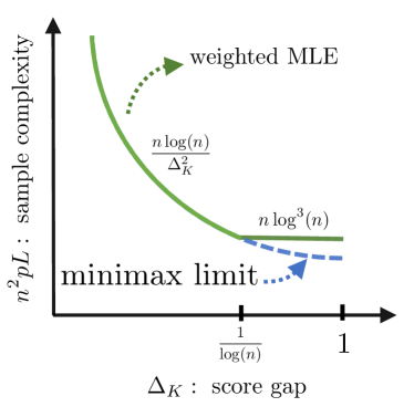
Figure 3: Sample complexity required to exactly recover top-$K$ items v.s. score gap $\Delta_{K}$. The solid line represent the required sample complexity of the weighted MLE as given in Theorem 1. The dashed line represents the minimax lower bound given in Theorem 2.

More precisely, when $\Delta_{K}\lesssim 1/\log(n)$, the weighted MLE requires $n^{2}pL\asymp n\log(n)/\Delta_{K}^{2}$ number of observations, which is exactly the minimax limit. On the other hand, when $1/\log(n)\lesssim\Delta_{K}\lesssim 1$, the weighted MLE needs $n^{2}pL\asymp n\log^{3}(n)$ comparisons, which exceeds the minimax lower bound by at most a $\log^{2}(n)$ factor.

Computational complexity.

Compared to a vanilla MLE, Algorithm 1 requires an additional reweighting step, which is performed by Algorithm 2. Crucially, we show that thsi step does not fundamentally alter the complexity of the whole procedure, as Algorithm 2 runs in nearly-linear time in the size of the graph $\mathcal{G}_{\mathrm{SR}}$. To ensure this fast running time, we combine the Matrix Multiplicative Weight Update (MMWU) framework [AK16] with a number of known approximation schemes, including fast computations of the action of the matrix exponential [OSV12], randomized dimensional reduction [Ach03] and fast solvers for packing linear programs [AZO18]. We also describe a simpler algorithm which does not require solving a packing linear program as a subroutine but relies on an easy-to-compute greedy approximation. This is the algorithm we implement in Section F.

Improved dependence on $\kappa$.

We remark in passing that compared to the $\ell_{\infty}$ bound $\|\widehat{\bm{\theta}}-\bm{\theta}^{\star}\|_{\infty}\lesssim\kappa^{2}\sqrt{\frac{\log(n)}{npL}}$ provided in [CFMW19], which is based on a probabilistic leave-one-out argument, our $\ell_{\infty}$ error bound (4) is tighter by a $\kappa$ factor.

3 Two algorithmic components

In this section we present the high-level analyses of the two algorithmic components in Algorithm 1, namely the weighted MLE, and the SDP-based reweigting method.

3.1 Weighted MLE

As the selected weight can be dependent on all edges of the comparison graph, we cannot use the popular and powerful leave-one-out technique in recent papers [CFMW19, CGZ22] to achieve entrywise control. Instead, we rely on and refine a new analysis for MLE [Che23] that is geared towards general graphs.

Recall that our estimator is a weighted MLE with weights $\{w_{ij}\}$ supported on the edges of the semi-random graph $\mathcal{G}_{\mathrm{SR}}$. Let $w_{\max}\coloneqq\max_{i,j}w_{ij}$ be the maximum weight, $d_{\max}\coloneqq\max_{i\in[m]}\sum_{j:j\neq i}w_{ij}$ be the maximum (weighted) degree, and $d_{\min}\coloneqq\min_{i\in[m]}\sum_{j:j\neq i}w_{ij}$ be the minimum (weighted) degree. In addition, we define the weighted graph Laplacian of $\mathcal{G}_{\mathrm{SR}}=(\mathcal{V},\mathcal{E}_{\mathrm{SR}},\{w_{ij}\})$ to be

$$\bm{L}_{w}\coloneqq\sum_{(i,j):i>j}w_{ij}(\bm{e}_{i}-\bm{e}_{j})(\bm{e}_{i}-\bm{e}_{j})^{\top}.$$ (5)

We have the following performance bounds for the weighted MLE whenever the weights are independent with the observed comparisons $\{y_{ij}\}$.

Theorem 3.

Suppose that the weighted graph $\mathcal{G}_{\mathrm{SR}}=(\mathcal{V},\mathcal{E}_{\mathrm{SR}},\{w_{ij}\})$ is connected. Assume that $w_{\max}\leq n^{2}$ and $d_{\min}\geq 1$. Further suppose that

$$L\geq C_{1}\frac{\kappa^{4}w_{\max}(d_{\max})^{4}\log^{2}(n)}{(\lambda_{n-1}(\bm{L}_{w}))^{5}}$$

for some large enough constant $C_{1}>0$. Then with probability at least $1-n^{-10}$, we have

$$\|\widehat{\bm{\theta}}-\bm{\theta}^{\star}\|_{\infty}\leq C_{2}\kappa\sqrt{\frac{w_{\max}\log(n)}{\lambda_{n-1}(\bm{L}_{w})L}},$$

where $C_{2}>0$ is a constant. On this event, the top-$K$ items are recovered exactly as long as

$$L\geq C_{3}\frac{\kappa^{2}w_{\max}\log(n)}{\lambda_{n-1}(\bm{L}_{w})\Delta_{K}^{2}}$$

for some large enough constant $C_{3}>0$.

See Section 4 for the proof of this theorem. Note that the assumptions on $w_{\max}$ and $d_{\min}$ are mild and stated only to simplify the log factor.

Theorem 3 provides an $\ell_{\infty}$ error bound for the weighted MLE under general comparison graphs. The bounds depend explicitly on the spectral properties of the weighted graph, including the maximum degree, and the spectral gap of the graph Laplacian.

An important by-product of our novel analysis of the weighted MLE is to demonstrate the optimal $\ell_{\infty}$ estimation error of the vanilla MLE in the uniform sampling case.

Corollary 1.

Consider the uniform sampling case, that is the comparison graph is an Erdős–Rényi graph. Assume that $\kappa=O(1)$, and that $p\gtrsim\log(n)/n$. The vanilla MLE with high probability achieves

$$\|\widehat{\bm{\theta}}-\bm{\theta}^{\star}\|_{\infty}\lesssim\sqrt{\frac{\log(n)}{npL}},$$

as long as $npL\gtrsim\log^{2}(n)$.

Proof.

Observe that the vanilla MLE is equivalent to the weighted MLE with a uniform weight $1$ on all the edges. With this choice, it is easy to show (see Lemma 10) that with high probability,

$$w_{\max} \leq 1,$$ (6a)

$$d_{\max} \leq 2np,$$ (6b)

$$\lambda_{n-1}(\bm{L}_{w}) \geq Cnp,$$ (6c)

where $C>0$ is some constant. Moreover by Lemma 14, $\lambda_{n-1}(\bm{L}_{w})\geq np/2$ together with $p\gtrsim\log(n)/n$ implies $d_{\min}\geq 1$. Apply Theorem 3 verbatim to arrive at the desired conclusion. ∎

3.2 An SDP-based reweighting

In view of the proof of Corollary 1, to mimic the vanilla MLE under uniform sampling, it is sufficient to construct the weights $\{w_{ij}\}$ such that the weighted graph $\mathcal{G}_{\mathrm{SR}}=(\mathcal{V},\mathcal{E}_{\mathrm{SR}},\{w_{ij}\})$ satisfies the spectral properties (6). In this section, we describe how to formulate this problem as a saddle-point semi-definite program (SDP) and approximately solve it in nearly-linear time in the size of $\mathcal{G}_{\mathrm{SR}}$ by designing a fast first-order method.

We formulate our task in terms of a convex optimization problem with variables $\{w_{ij}\in\mathbb{R}\}_{(i,j)\in\mathcal{E}_{\mathrm{SR}}}$ representing our desired reweighting. The convex feasible set $\mathcal{F}$ for such weights is given by the rescaled Equations (6b) and (6c):

$$\mathcal{F}\coloneqq\{\bm{w}\in\mathbb{R}^{\mathcal{E}_{\mathrm{SR}}}_{\geq 0}:\forall i\in\mathcal{V},\sum_{j:(i,j)\in\mathcal{E}_{\mathrm{SR}}}w_{ij}\leq 2np\;\land\;\forall(i,j)\in\mathcal{E}_{\mathrm{SR}},w_{ij}\leq 1\}.$$ (7)

For a choice of weights $\bm{w}$, we denote by $\bm{L}_{\bm{w}}$ the corresponding weighted Laplacian as defined in (5). With this notation, we consider the problem of maximizing the spectral gap $\lambda_{n-1}(\bm{L}_{\bm{w}})$ over $\bm{w}\in\mathcal{F}$. It is a well-known fact that this is a convex optimization problem in the variables $\bm{w}$ [BDX04]. Indeed, we can write $\lambda_{n-1}(\bm{L}_{\bm{w}})$ as the minimum of the matrix inner product $\langle\bm{L}_{\bm{w}},\bm{X}\rangle$ over $\bm{X}$ in the set

$$\Delta\coloneqq\{\bm{X}\in\mathbb{S}^{\mathcal{V}}:\bm{X}\succeq 0\;\land\;\langle\Pi_{\perp\bm{1}},\bm{X}\rangle=1\},$$

where $\mathbb{S}^{\mathcal{V}}$ is the set of symmetric linear operators over $\mathcal{V}$ and $\Pi_{\perp\bm{1}}$ is the orthogonal projector over the orthogonal complement of the vector $\bm{1}$, which is the eigenvector of $\bm{L}_{\bm{w}}$ with the smallest eigenvalue. Therefore, our desired convex optimization problem can be recast as the following saddle point problem between an SDP variable $\bm{X}$ and the weight $\bm{w}$. This formulation will be crucial for the solvers designed in the later section:

$$\mathrm{OPT}\coloneqq\max_{\bm{w}\in\mathcal{F}}\min_{\bm{X}\in\Delta}\quad\langle\bm{L}_{\bm{w}},\bm{X}\rangle.$$ (Saddle-Point SDP)

By considering the weighting $\bm{w}$ corresponding to the original graph in $\mathcal{G}_{\mathrm{ER}}$ as a feasible reweighting for Saddle-Point SDP, the proof of Corollary 1 immediately implies a lower bound on $\mathrm{OPT}$: with probability at least $1-n^{-10}$,

$$\mathrm{OPT}\geq\frac{np}{2},$$ (8)

as long as $p\geq C\log(n)/n$ for some sufficiently large constant $C>0$.

While it is not always possible to recover the underlying graph $\mathcal{G}_{\mathrm{ER}}$, the lower bound (8) ensures that, by approximately solving Saddle-Point SDP, we can find a reweighting of $\mathcal{G}_{\mathrm{SR}}$ that satisfies the required spectral properties (6). The next lemma, proved in Section 5, shows that this approximate solution can be computed in nearly-linear time in the size of $\mathcal{G}_{\mathrm{SR}}$. The corresponding algorithm, Algorithm 2 to be detailed in Section 5, is based on the Matrix Multiplicative Weight Update (MMWU) framework [AK16], a first-order method for non-smooth convex SDP optimization.

Lemma 1.

Given the observed comparison graph $\mathcal{G}_{\mathrm{SR}}$, there is an algorithm that computes a set of non-negative weights $\left\{w_{ij}\right\}_{i>j}$ supported on $\mathcal{E}_{\mathrm{SR}}$ that satisfy the properties (6) with high probability. In addition, the algorithm runs in nearly-linear time in the size of $\mathcal{G}_{\mathrm{SR}}.$

We finish this section by noting that once the spectral properties are met, repeating the proof of Corollary 1 yields the desired results in Theorem 1 in the semi-random case.

4 Analysis of weighted MLE

In this section, we present detailed analysis of the weighted MLE with the aim of proving Theorem 3.

Given a set of weights $\{w_{ij}\}$, the Hessian of the weighted loss at ground truth is given by

$$\nabla^{2}\mathcal{L}(\bm{\theta}^{\star})=\sum_{(i,j):i>j}w_{ij}\underbrace{\frac{e^{\theta_{i}^{\star}}e^{\theta_{j}^{\star}}}{(e^{\theta_{i}^{\star}}+e^{\theta_{j}^{\star}})^{2}}}_{\eqqcolon z_{ij}}(\bm{e}_{i}-\bm{e}_{j})(\bm{e}_{i}-\bm{e}_{j})^{\top}.$$

This is exactly the graph Laplacian of the weighted graph $\mathcal{G}_{\mathrm{SR}}$ with weights $\{w_{ij}z_{ij}\}$. Hence we denote this by $\bm{L}_{wz}$. We also define the effective resistance to be

$$\bm{\Omega}_{kl}(\bm{L}_{wz})\coloneqq(\bm{e}_{k}-\bm{e}_{l})^{\top}\bm{L}_{wz}^{\dagger}(\bm{e}_{k}-\bm{e}_{l}),$$

where $\bm{L}_{wz}^{\dagger}$ is the pseudo-inverse of $\bm{L}_{wz}$.

Inspired by Theorem 1 in the paper [Che23], the first step of the proof relates the performance of the weighted MLE with two crucial quantities $\{B_{kl}\}$ and $\{Q_{kl}\}$.

Lemma 2.

Suppose that the weighted graph $(\mathcal{V},\mathcal{E}_{\mathrm{SR}},\{w_{ij}\})$ is connected by edges of non-zero weight and the weights $\{w_{ij}\}$ are independent with the observations $\{y_{ij}\}$. For any $(k,l)\in[n]^{2},k\neq l$, let $B_{kl}$ and $Q_{kl}$ be some quantities obeying

$$B_{kl} \geq C\sqrt{\frac{\kappa}{L}\left(\max_{i,j}w_{ij}\right)\bm{\Omega}_{kl}(\bm{L}_{wz})\log(n)};$$ (9a)

$$Q_{kl} \geq\sum_{(i,j):i>j}w_{ij}B_{ij}^{2}\left|(\bm{e}_{k}-\bm{e}_{l})^{\top}\bm{L}_{wz}^{\dagger}(\bm{e}_{i}-\bm{e}_{j})\right|.$$ (9b)

Here $C>0$ is some large enough constant. Suppose that $Q_{kl}\leq 4B_{kl}$ for any $(k,l)$. Then with probability at least $1-n^{-10}$, we have that for any $(k,l)\in[n]^{2}$,

$$\|\widehat{\bm{\theta}}-\bm{\theta}^{\star}\|_{\infty}\leq B_{kl}.$$

On this event, the top-$K$ items are recovered exactly as long as

$$\max_{k,l}B_{kl}\leq\Delta_{K}/2.$$

Admittedly, the two quantities $\{B_{kl}\}$ and $\{Q_{kl}\}$ appearing in the performance bound of MLE is quite mysterious. A key contribution of this paper is to further relate these two quantities to basic spectral properties of the weighted graph $(\mathcal{V},\mathcal{E}_{\mathrm{SR}},\{w_{ij}\})$. We start with the characterization of $B_{kl}$. Recall that $w_{\max}=\max_{i,j}w_{ij}$ is the maximum weight.

Lemma 3.

For any $(k,l)\in[n]^{2}$, the effective resistance $\Omega_{kl}(\bm{L}_{wz})$ satisfies

$$\Omega_{kl}(\bm{L}_{wz})\leq\frac{8\kappa}{\lambda_{n-1}(\bm{L}_{w})}.$$

As a result, it is sufficient to take

$$B_{kl}=C\kappa\sqrt{\frac{w_{\max}\log(n)}{L\lambda_{n-1}(\bm{L}_{w})}},$$

where $C>0$ is some large enough constant.

Now we move on to controlling the $Q$ factors via spectral properties of the weighted graph. Recall $d_{\max}=\max_{i\in[m]}\sum_{j:j\neq i}w_{ij}$ is the maximum (weighted) degree and $d_{\min}=\min_{i\in[m]}\sum_{j:j\neq i}w_{ij}$ is the minimum (weighted) degree. We have the following bound.

Lemma 4.

Suppose that $w_{\max}\leq n^{2}$ and that $d_{\min}\geq 1$. Then for any $(k,l)\in[n]^{2}$, we have

$$\sum_{(i,j):i>j}w_{ij}\left|(\bm{e}_{k}-\bm{e}_{l})^{\top}\bm{L}_{wz}^{\dagger}(\bm{e}_{i}-\bm{e}_{j})\right|\leq C\kappa\cdot\frac{(d_{\max})^{2}\log(n)}{(\lambda_{n-1}(\bm{L}_{w}))^{2}},$$

where $C_{1}>0$ is some constant. As a result, it is sufficient to take

$$Q_{kl}=C_{2}\kappa^{3}\cdot\frac{w_{\max}(d_{\max})^{2}\log^{2}(n)}{L(\lambda_{n-1}(\bm{L}_{w}))^{3}}$$

for some large enough constant $C_{2}>0$.

Combining Lemmas 3-4, we see that $Q_{kl}\leq 4B_{kl}$ holds as long as

$$L\geq C_{3}\frac{\kappa^{4}w_{\max}(d_{\max})^{4}\log^{2}(n)}{(\lambda_{n-1}(\bm{L}_{w}))^{5}}$$

for some large enough constant $C_{3}>0$. This together with Lemma 2 completes the proof of Theorem 3. In what follows, we present the proofs of Lemmas 3-4, and defer the proof of Lemma 2 to Appendix B.

4.1 Proof of Lemma 3

Recall that $\bm{\Omega}_{kl}(\bm{L}_{wz})=(\bm{e}_{k}-\bm{e}_{l})^{\top}\bm{L}_{wz}^{\dagger}(\bm{e}_{k}-\bm{e}_{l})$, which implies

$$\bm{\Omega}_{kl}(\bm{L}_{wz})\leq 2\|\bm{L}_{wz}^{\dagger}\|=\frac{2}{\lambda_{n-1}(\bm{L}_{wz})}.$$

Regarding $\lambda_{n-1}(\bm{L}_{wz})$, by definition, one has

$$\lambda_{n-1}(\bm{L}_{wz}) =\inf_{\bm{v}\in\mathbb{R},\|\bm{v}\|=1,\bm{v}\perp\bm{1}_{n}}\bm{v}^{\top}\bm{L}_{wz}\bm{v}$$

$$=\inf_{\bm{v}\in\mathbb{R},\|\bm{v}\|=1,\bm{v}\perp\bm{1}_{n}}\bm{v}^{\top}\left[\sum_{(i,j):i>j}w_{ij}z_{ij}(\bm{e}_{i}-\bm{e}_{j})(\bm{e}_{i}-\bm{e}_{j})^{\top}\right]\bm{v}$$

$$\geq\frac{1}{4\kappa}\inf_{\bm{v}\in\mathbb{R},\|\bm{v}\|=1,\bm{v}\perp\bm{1}_{n}}\bm{v}^{\top}\left[\sum_{(i,j):i>j}w_{ij}(\bm{e}_{i}-\bm{e}_{j})(\bm{e}_{i}-\bm{e}_{j})^{\top}\right]\bm{v}$$

$$=\frac{1}{4\kappa}\lambda_{n-1}(\bm{L}_{w}),$$ (10)

where the inequality follows from Lemma 9.

4.2 Proof of Lemma 4

For readers’ convenience, we copy the key quantity appearing in Lemma 4 below:

$$\sum_{(i,j):i>j}w_{ij}\left|(\bm{e}_{k}-\bm{e}_{l})^{\top}\bm{L}_{wz}^{\dagger}(\bm{e}_{i}-\bm{e}_{j})\right|.$$ (11)

It turns out that this quantity is closely related to the so-called conductance of the weighted graph defined as follows.

Definition 1 (Conductance).

For a weighted graph $\mathcal{G}=(\mathcal{V},\mathcal{E},w)$, we define its conductance to be

$$\Phi(\mathcal{G})\coloneqq\min_{\mathcal{S}\subset\mathcal{V}}\frac{\sum_{i\in\mathcal{S},j\in\mathcal{V}\setminus\mathcal{S}}w_{ij}}{\min\{\mathrm{vol}(\mathcal{S}),\mathrm{vol}(\mathcal{V}\setminus\mathcal{S})\}},$$

where the volume of a vertex set $\mathcal{S}\subset\mathcal{V}$ is defined by

$$\mathrm{vol}(\mathcal{S})\coloneqq\sum_{i\in\mathcal{S}}\sum_{j\in\mathcal{V}:j\neq i}w_{ij}.$$

The following lemma links the quantity in (11) with graph conductance. This lemma is modified from Lemma 28 in [KLOS14]. The proof is deferred to Section C.

Lemma 5.

Consider a graph $\mathcal{G}=(\mathcal{V},\mathcal{E})$ equipped with two set of weights $\{w_{ij}\}$ and $\{\widetilde{w}_{ij}\}$ both supported on $\mathcal{E}$. Suppose that the minimum $\{w_{ij}\}$-weighted degree is at least 1. Then one has

$$\sum_{(i,j):i>j}w_{ij}\left|(\bm{e}_{i}-\bm{e}_{j})^{\top}\bm{L}_{\mathcal{G}_{\widetilde{w}}}^{\dagger}(\bm{e}_{k}-\bm{e}_{l})\right|\leq\max_{(i,j)\in\mathcal{E}}\left\{\frac{w_{ij}}{\widetilde{w}_{ij}}\right\}\cdot\frac{8\log\left(\sum_{(i,j):i>j}w_{ij}\right)}{\Phi(\mathcal{G}_{w})^{2}}.$$ (12)

Set $\tilde{w}_{ij}=w_{ij}z_{ij}$. We can apply Lemma 5 to obtain

$$\sum_{(i,j):i>j}w_{ij}\left|(\bm{e}_{i}-\bm{e}_{j})^{\top}\bm{L}_{wz}^{\dagger}(\bm{e}_{k}-\bm{e}_{l})\right| \leq\max_{(i,j):w_{ij}>0}\left\{\frac{w_{ij}}{w_{ij}z_{ij}}\right\}\cdot\frac{8\log\left(\sum_{(i,j):i>j}w_{ij}\right)}{\Phi(\mathcal{G}_{w})^{2}}$$

$$\leq 4\kappa\cdot\frac{8\log\left(\sum_{(i,j):i>j}w_{ij}\right)}{\Phi(\mathcal{G}_{w})^{2}},$$

where the last inequality again follows from Lemma 9.

For the numerator, since $w_{\max}\leq n^{2}$, we have $\log(\sum_{(i,j):i>j}w_{ij})\leq 3\log(n)$. Now we focus on the denominator, i.e., the graph conductance. It is well known that the graph conductance is controlled by the eigenvalue of the normalized Laplacian (see Lemma 11), that is

$$\Phi(\mathcal{G}_{w})\geq\frac{1}{2}\lambda_{n-1}\left(\bm{D}_{w}^{-1/2}\bm{L}_{w}\bm{D}_{w}^{-1/2}\right),$$

where $\bm{D}_{w}$ is a diagonal matrix composed of the weighted degrees. By Sylvester’s law of inertia (Lemma 13), we further have

$$\lambda_{n-1}\left(\bm{D}_{w}^{-1/2}\bm{L}_{w}\bm{D}_{w}^{-1/2}\right) \geq\lambda_{n}\left(\bm{D}_{w}^{-1}\right)\lambda_{n-1}\left(\bm{L}_{w}\right)=(d_{\max})^{-1}\cdot\lambda_{n-1}\left(\bm{L}_{w}\right).$$

Taking the above bounds collectively yields the desired claim in Lemma 4.

Algorithm 2 MMWU algorithm for Saddle-Point SDP

0:  Graph $\mathcal{G}_{\mathrm{SR}}=(V,\mathcal{E}_{\mathrm{SR}})$, $|V|=n$, $|\mathcal{E}_{\mathrm{SR}}|=m,$ error parameter $\epsilon\in(0,\nicefrac{{1}}{{2}}]$.

1:  $\bm{w}^{(0)}=\bm{0},\eta=\nicefrac{{\epsilon}}{{4pn}},k=O\left(\nicefrac{{\log(n)}}{{\epsilon^{2}}}\right),$ $T=\nicefrac{{8\log(n)}}{{\epsilon^{2}}}$

2:  for $t=0,\ldots,T-1$ do

3:     Sample $\bm{R}=\{\pm\nicefrac{{1}}{{\sqrt{k}}}\}^{n\times k}$ uniformly at random. // $\{\pm 1\}$ JL matrix with $\nicefrac{{1}}{{\sqrt{k}}}$ scaling [Ach03]

4:     Compute $\bm{U}^{(t)}=\exp\{-\eta\sum_{ij\in\mathcal{E}_{\mathrm{SR}}}{w}^{(t)}_{ij}\bm{L}_{ij}\}\bm{R}.$ // Use matrix exponentiation in [AK16]

5:     Compute $\bm{V}^{(t)}=\nicefrac{{\bm{U}^{(t)}}}{{\sqrt{\langle\Pi_{\perp\bm{1}},\bm{U}^{(t)}(\bm{U}^{(t)})^{T}\rangle}}}$.// MMWU Normalization

6:     For each $ij\in\mathcal{E}_{\mathrm{SR}}$, let $c_{ij}=\langle\bm{L}_{ij},\bm{V}^{(t)}(\bm{V}^{(t)})^{T}\rangle$. // Compute edge gains

7:     Compute $\hat{\bm{w}}^{(t)}\in\mathcal{F}$, an $\epsilon$- or $\nicefrac{{1}}{{2}}$-approximate solution to $\max_{\bm{w}\in\mathcal{F}}\langle\bm{c},\bm{w}\rangle.$ // Use Theorem 4 or 5

8:     Update $\bm{w}^{t+1}=\bm{w}^{(t)}+\hat{\bm{w}}^{(t)}.$

9:  end for

9:  Edge weighting $\bm{w}_{\mathrm{out}}=\nicefrac{{1}}{{T}}\cdot\sum_{t=0}^{T-1}\bm{w}^{(t)}.$

5 Analysis of SDP-based reweighting

In this section, we describe and analyze the MMWU algorithm for solving the reweighting SDP problem  Saddle-Point SDP in Section 3.2. We conclude by proving Lemma 1.

5.1 MMWU algorithm for Saddle-Point SDP

We present the pseudocode for the the MMWU Algorithm in Algorithm 2. Our algorithm instantiates the MMWU framework of Arora and Kale [AK16], where we avoid maintaining full $|\mathcal{V}|\times|\mathcal{V}|$ matrices by relying on the Johnson-Lindestrauss Lemma [Ach03] (see lines 3 and 4).

At every iteration, the MMWU algorithm produces a candidate solution $\bm{X}^{(t)}\in\Delta$ to which we respond with a loss matrix $\bm{L}^{(t)}\coloneqq\bm{L}_{\bm{w}^{(t)}}=\sum_{ij\in\mathcal{E}_{\mathrm{SR}}}w_{ij}^{(t)}\bm{L}_{ij}$ with $\bm{w}^{(t)}\in\mathcal{F}$, where $\bm{L}_{ij}\coloneqq(\bm{e}_{i}-\bm{e}_{j})(\bm{e}_{i}-\bm{e}_{j})^{\top}$. In this way, the loss $\langle\bm{L}^{(t)},\bm{X}^{(t)}\rangle$ incurred by the MMWU algorithm at iteration $t$ equals the value of Saddle-Point SDP on the pair of solutions $(\bm{X}^{(t)},\bm{w}^{(t)}).$ At every iteration $t,$ given $\bm{X}^{(t)}$, our goal is then to choose $\bm{w}^{(t)}\in\mathcal{F}$ to maximize the loss $\langle\bm{L}^{(t)},\bm{X}^{(t)}\rangle$. The regret minimization property of MMWU then allows us to turn this per-iteration guarantee into a global guarantee on $\lambda_{n-1}(\sum_{t=0}^{T-1}\bm{L}^{(t)})$.

To maximize the loss of the MMWU algorithm, we choose $\bm{w}^{(t)}\in\mathcal{F}$ to approximate the best response $\max_{\bm{w}\in\mathcal{F}}\langle\bm{L}_{\bm{w}},\bm{X}^{(t)}\rangle.$ We describe two algorithms (oracles in the language of [AK16]) for approximately solving this task. The first one is based on directly applying a nearly-linear-time packing LP solver. It is described in Appendix D and yields the following theorem.

Theorem 4.

Given $\bm{X}\in\Delta,$ one can $(1-\epsilon)$-approximate $\max\limits_{\bm{w}\in\mathcal{F}}\langle\bm{L}_{\bm{w}},\bm{X}\rangle$ multiplicatively in time $\tilde{O}(\nicefrac{{|\mathcal{E}_{\mathrm{SR}}|}}{{\epsilon}}).$

Our second oracle exploits the fact that $\max_{\bm{w}\in\mathcal{F}}\langle\bm{L}_{\bm{w}},\bm{X}\rangle=\max_{\bm{w}\in\mathcal{F}}\langle\bm{c},\bm{w}\rangle$ is a LP relaxation of the maximum weight $b$-matching problem over $\mathcal{G}_{\mathrm{SR}}$ with edge weights $\bm{c}$. We can approximate the maximum weight $b$-matching by a greedy procedure: iterate through the edges of $\mathcal{E}_{\mathrm{SR}}$ once in decreasing order of edge gains $c_{ij}=\langle\bm{L}_{ij},\bm{X}\rangle$, and add an edge so long as both adjacent vertices possess available demand. Though this only achieves a $\nicefrac{{1}}{{2}}$-approximation [Mes06], the simplicity of the algorithm makes it extremely suitable for implementation. We prove the following theorem in Appendix D.

Theorem 5.

Given $\bm{X}\in\Delta,$ one can $\nicefrac{{1}}{{2}}$-approximate $\max_{\bm{w}\in\mathcal{F}}\langle\bm{L}_{\bm{w}},\bm{X}\rangle$ multiplicatively in time $\tilde{O}(|\mathcal{E}_{\mathrm{SR}}|).$

5.2 Analysis of Algorithm 2

We are now ready to prove Lemma 1. To analyze the correctness and running time of Algorithm 2, we first recall the regret bound achieved by applying MMWU to the vector space $\mathbb{R}^{V}\perp\bm{1}$.

Theorem 6 (Theorem 3.1 [AK16]).

Consider a sequence of loss matrices $\{\bm{L}^{(t)}\in\mathbb{S}^{V}\}_{t\in[T]}$ with $\bm{L}^{(t)}\bm{1}=0$ for all $t$. Let

$$\bm{W}^{(t)}=\exp\left\{-\eta\sum_{s=0}^{t-1}\bm{L}^{(s)}\right\},\quad\text{ and }\quad\bm{X}^{(t)}=\frac{\bm{W}^{(t)}}{\langle\Pi_{\perp\bm{1}},\bm{W}^{(t)}\rangle}.$$

Then, we have the regret bound:

$$\min_{\bm{X}\in\Delta}\left\langle\sum_{t=0}^{T-1}\bm{L}^{(t)},\bm{X}\right\rangle\geq\sum_{t=0}^{T-1}\langle\bm{L}^{(t)},\bm{X}^{(t)}\rangle-\eta\sum_{s=0}^{T-1}\langle(\bm{L}^{(t)})^{2},\bm{X}^{(t)}\rangle-\frac{\log(n)}{\eta}.$$ (13)

Next, we use Lemma 6 to show that $\bm{V}^{(t)}$, produced by Algorithm 2, approximate the MMWU updates $\bm{X}^{(t)}$ in Theorem 6 when computing the squared distances $\langle\bm{L}_{ij},\bm{X}^{(t)}\rangle$. This is proven in Appendix D.2.

Lemma 6.

Let $\tilde{\bm{X}}^{(t)}=\bm{V}^{(t)}(\bm{V}^{(t)})^{T}$ as defined in Algorithm 2. Then, $\tilde{\bm{X}}^{(t)}\in\Delta.$ Moreover, for large enough $k\in O(\nicefrac{{\log(n)}}{{\epsilon^{2}}})$, for all pairs $(i,j)\in\mathcal{V}\times\mathcal{V}$, the squared distance $\langle\bm{L}_{ij},\tilde{\bm{X}}^{(t)}\rangle$ is an $\epsilon$-multiplicative approximation to the squared distance $\langle\bm{L}_{ij},\bm{X}^{(t)}\rangle$ with high probability.

We can use the above to establish the algorithm’s correctness; we prove the following lemma in Section 5.3.

Lemma 7.

With high probability, Algorithm 2 outputs a reweighting $\bm{w}_{\mathrm{out}}\in\mathcal{F}$ of $\mathcal{G}_{\mathrm{SR}}$ such that

$$\min_{\bm{X}\in\Delta}\langle\bm{L}_{\bm{w}_{\mathrm{out}}},\bm{X}\rangle\geq\begin{cases}(1-O(\epsilon))\cdot\mathrm{OPT},&\textrm{ if Theorem\leavevmode\nobreak\ \ref{thm:LP-oracle} is used in line\leavevmode\nobreak\ \ref{line:oracle}},\\ (\nicefrac{{1}}{{2}}-O(\epsilon))\cdot\mathrm{OPT},&\textrm{ if Theorem\leavevmode\nobreak\ \ref{thm:greedy-oracle} is used in line\leavevmode\nobreak\ \ref{line:oracle}}.\\ \end{cases}$$

Finally, we can bound the running time of Algorithm 2 using known algorithms for computing the action of the matrix exponential [AK16, OSV12]. The proof of the next lemma is also given in Appendix D.2.

Lemma 8.

For a constant $\epsilon>0,$ Algorithm 2 runs in nearly-linear time in the size of $\mathcal{G}_{\mathrm{SR}}$.

Combining Lemmata 7 and 8 yields our main result on the reweighting of $\mathcal{G}_{\mathrm{SR}}$, i.e., Lemma 1.

Proof of Lemma 1.

We claim that the output $\bm{w_{\mathrm{out}}}$ of Algorithm 2 satisfies the required properties. The conditions of (6b) and (6a) are immediately satisfied by the fact that $\bm{w_{\mathrm{out}}}\in\Delta$, which is proved in Lemma 7. The spectral condition in (6c) follows from the approximation guarantee of Lemma 7 and the lower bound (8):

$$\lambda_{n-1}\left(\bm{L}_{\bm{w}_{\mathrm{out}}}\right)=\cdot\min_{\bm{X}\in\Delta}\langle\bm{L}_{\bm{w}_{\textrm{out}}},\bm{X}\rangle\geq\Omega\left(\mathrm{OPT}\right)\geq\Omega(np).$$

The nearly-linear running time is proved in Lemma 8. ∎

5.3 Proof of Lemma 7

Notice that $\bm{w}_{\textrm{out}}\in\mathcal{F}$ as it is the average of elements of $\mathcal{F}$ and $\mathcal{F}$ is convex. Moreover, we have $\bm{L}_{\bm{w}_{\textrm{out}}}=\nicefrac{{1}}{{T}}\cdot\sum_{t=0}^{T-1}\bm{L}_{\bm{w}^{(t)}}=\nicefrac{{1}}{{T}}\cdot\sum_{t=0}^{T-1}\bm{L}^{(t)}.$ By the regret bound in Equation (13), we then obtain:

$$\min_{\bm{X}\in\Delta}\langle\bm{L}_{\bm{w}_{\textrm{out}}},\bm{X}\rangle\geq\frac{1}{T}\left(\sum_{t=0}^{T-1}\langle\bm{L}_{\bm{w}^{(t)}},\bm{X}^{(t)}\rangle\right)-\frac{\eta}{T}\left(\sum_{s=0}^{T-1}\langle(\bm{L}_{\bm{w}^{(t)}})^{2},\bm{X}^{(t)}\rangle\right)-\frac{\log(n)}{\eta T}.$$ (14)

We can exploit the positive semi-definiteness of $\bm{L}_{\bm{w}^{(t)}}$ to bound the second term as a function of the first. By the definition of $\mathcal{F}$, the reweighting of $\mathcal{G}$ by $\bm{w}^{(t)}\in\mathcal{F}$ has maximum degree at most $2pn.$ Hence:

$$\bm{L}_{\bm{w}^{(t)}}\preceq 2\cdot 2pn\cdot\Pi_{\perp\bm{1}}\textrm{ and }\langle(\bm{L}_{\bm{w}^{(t)}})^{2},\bm{X}^{(t)}\rangle\leq 4pn\cdot\langle\bm{L}_{\bm{w}^{(t)}},\bm{X}^{(t)}\rangle.$$

We can now rewrite Equation (14) as:

$$\min_{\bm{X}\in\Delta}\langle\bm{L}_{\bm{w}_{\textrm{out}}},\bm{X}\rangle\geq\left(\frac{1}{T}-\frac{4pn\cdot\eta}{T}\right)\left(\sum_{t=0}^{T-1}\langle\bm{L}_{\bm{w}^{(t)}},\bm{X}^{(t)}\rangle\right)-\frac{\log(n)}{\eta T}.$$

For all iterations $t$, we have:

$$\langle\bm{L}_{\bm{w}^{(t)}},\bm{X}^{(t)}\rangle\geq(1-\epsilon)\langle\bm{L}_{\bm{w}^{(t)}},\tilde{\bm{X}}^{(t)}\rangle=(1-\epsilon)\sum_{ij\in\mathcal{E}_{\mathrm{SR}}}w_{ij}^{(t)}\langle\bm{L}_{ij},\bm{V}^{(t)}(\bm{V}^{(t)})^{T}\rangle=(1-\epsilon)\max_{\bm{w}\in\mathcal{F}}\langle\bm{L}_{\bm{w}},\tilde{\bm{X}}^{(t)}\rangle,$$

where the first inequality follows from Lemma 6 and the last equality follows from Lines 6 and 7 in Algorithm 2. As $\tilde{\bm{X}}^{(t)}\in\Delta$, the maximum in the last expression has value at least $\mathrm{OPT}$. Hence, for the two oracles of Theorems 4 and 5, we have:

$$\mathrm{Theorem\leavevmode\nobreak\ \ref{thm:LP-oracle}:}\langle\bm{L}_{\bm{w}^{(t)}},\bm{X}^{(t)}\rangle\geq(1-\epsilon)^{2}\cdot\mathrm{OPT}\;\mathrm{and\leavevmode\nobreak\ Theorem\leavevmode\nobreak\ \ref{thm:greedy-oracle}:}\langle\bm{L}_{\bm{w}^{(t)}},\bm{X}^{(t)}\rangle\geq\frac{(1-\epsilon)}{2}\cdot\mathrm{OPT}.$$

Therefore:

$$\min_{\bm{X}\in\Delta}\langle\bm{L}_{\bm{w}_{\textrm{out}}},\bm{X}\rangle\geq\begin{cases}(1-4pn\cdot\eta)\cdot(1-\epsilon)^{2}\cdot\mathrm{OPT}-\frac{\log(n)}{\eta T}\\ (1-4pn\cdot\eta)\cdot\frac{(1-\epsilon)}{2}\cdot\mathrm{OPT}-\frac{\log(n)}{\eta T}\\ \end{cases}$$

Substituting the definitions of $\eta=\nicefrac{{\epsilon}}{{4pn}}$ yields:

$$\min_{\bm{X}\in\Delta}\langle\bm{L}_{\bm{w}_{\textrm{out}}},\bm{X}\rangle\geq\begin{cases}(1-\epsilon)^{3}\cdot\mathrm{OPT}-\frac{4pn\log(n)}{\epsilon T}\\ \frac{(1-\epsilon)^{2}}{2}\cdot\mathrm{OPT}-\frac{4pn\log(n)}{\epsilon T}\\ \end{cases}$$

By the lower bound (8), the last term in both expressions can be upper bound by $\nicefrac{{8\mathrm{OPT}\log(n)}}{{\epsilon T}}.$ The statement of the lemma follows from the definition $T=\nicefrac{{8\log(n)}}{{\epsilon^{2}}}.$

6 Discussion

In this paper we consider top-$K$ ranking with a monotone adversary. We carefully construct a weighted MLE that achieves the optimal $\ell_{\infty}$ estimation error and top-$K$ recovery sample complexity. This leaves open quite a few interesting directions. We single out several of them below.

• Shaving the $\log^{2}(n)$ factor. Compared to the results for uniform sampling, ours requires an extra assumption that $npL\gtrsim\log^{3}(n)$. While this is optimal for a wide range of $\Delta_{K}$, it does incur an extra $\log^{2}(n)$ factor when $1/\log(n)\lesssim\Delta_{K}\lesssim 1$. We do not expect this to be the fundamental gap between uniform sampling and semi-random sampling. Successfully shaving this extra log factor will potentially bring more insights to understanding the geometry of the comparison graph on the ranking problem.

• Is weighted MLE necessary? While our approach relies on the weighted MLE, it is not clear whether the unweighted vanilla MLE succeeds or not with a monotone adversary. In fact, in Appendix E, we present a specific example of semi-random sampling where the spectral properties of the semi-random graph are drastically different from those of random graph, yet the vanilla MLE still succeeds.

• Extension to general graphs. Theorem 1 in [Che23] and Theorem 2 in our paper both consider general comparison graphs. Our analysis can recover a good rate with small sample complexity when the spectrum of the comparison graph has small dynamic range, i.e. $\lambda_{1}/\lambda_{n-1}$ is small. Our reweighting procedure indicates that any comparison graph which can be reweighted to match this spectral condition will yield small sample complexity. It is an interesting question to explore the connection between the reweighting SDP and similar SDPs used in the approximation of general partitioning objectives [LTW23] to find novel combinatorial or geometric properties enabling the success of the weighted MLE.

• Extensions to other ranking models. In this paper we focus on one of the most popular model in ranking, namely the BTL model. It is certainly interesting to see whether our algorithm and analysis for semi-random sampling can be extended to other models, for instance the Thurstone model [Thu27], the Plackett-Luce model [Luc05], and other models for multi-way comparisons [FLWY22, FLWY23].

Acknowledgements

AC is supported by NSF DGE 2140001. LO is supported by NSF CAREER 1943510. CM was partially supported by the National Science Foundation via grant DMS-2311127.

Appendix A Auxiliary lemmas

This section collects several auxiliary lemmas we use in the proofs of our main results.

Lemma 9 (Range of $z_{ij}$).

Recall that

$$z_{ij}=\frac{e^{\theta_{i}^{\star}}e^{\theta_{j}^{\star}}}{(e^{\theta_{i}^{\star}}+e^{\theta_{j}^{\star}})^{2}}=\frac{e^{\theta_{i}^{\star}-\theta_{j}^{\star}}}{(1+e^{\theta_{i}^{\star}-\theta_{j}^{\star}})^{2}}.$$

We have for any $i,j$,

$$\frac{1}{4\kappa}\leq z_{ij}\leq\frac{1}{4}.$$

Proof.

The function $f(x)=x/(1+x)^{2}$ has derivative $(1-x^{2})/(1+x)^{4}$ so it is increasing in $(0,1)$ and decreasing in $(1,\infty)$. Furthermore from the definition of $\kappa$, $|\theta_{i}^{\star}-\theta_{j}^{\star}|\leq\log(\kappa)$. Then we have

$$\frac{1}{4\kappa}\leq\min\left\{f(\kappa),f(1/\kappa)\right\}\leq z_{ij}\leq f(1)=\frac{1}{4}.$$

This completes the proof. ∎

Lemma 10 (spectral gap of a Erdős-Rényi graph).

Let $\mathcal{G}=([n],\mathcal{E})\sim G(n,p)$ be an Erdős-Rényi graph with $n$ vertices and edge probability $p$. Let $\bm{L}$ be its corresponding graph Laplacian matrix. Let $d_{\max}$ be the maximum degree of the vertices. Suppose that $np\geq C\log(n)$ for some large enough constant $C>0$, then with probability at least $1-n^{-10}$,

$$\lambda_{n-1}(\bm{L}) \geq\frac{np}{2}$$

$$d_{\max} \leq 2np.$$

Proof.

See, for instance, Section 5.3.3 of [Tro15]. ∎

Lemma 11 ([Spi07]).

Let $\mathcal{G}$ be a weighted graph and $\Phi(\mathcal{G})$ be its conductance (see Definition 1). Let $\bm{L}$ be its graph Laplacian matrix. Let $\bm{D}$ be the diagonal matrix with the weighted vertex degrees as the entries. Then

$$\Phi(\mathcal{G})\geq\frac{1}{2}\lambda_{n-1}(\bm{D}^{-1/2}\bm{L}\bm{D}^{-1/2}).$$

Lemma 12 (Rayleigh’s monotonicty law, [Bol98] Corollary 7 in Ch.IX).

Let $\mathcal{G}=(\mathcal{V},\mathcal{E})$ be a graph with weights $\{w_{ij}\}$ on $\mathcal{E}$, and $\widetilde{\mathcal{G}}=(\mathcal{V},\widetilde{\mathcal{E}})$ be a graph with weights $\{\widetilde{w}_{ij}\}$ on $\widetilde{\mathcal{E}}$. Suppose that $\mathcal{E}\subset\widetilde{\mathcal{E}}$ and $w_{ij}\leq\widetilde{w}_{ij}$ for any $(i,j)\in\mathcal{E}$, then for any $(k,l)\in\mathcal{V}^{2}$, the effective resistance satisfies

$$\bm{\Omega}_{kl}(\bm{L}_{\mathcal{G}_{w}})\leq\bm{\Omega}_{kl}(\bm{L}_{\widetilde{\mathcal{G}}_{\widetilde{w}}}).$$

Lemma 13 (A quantitative version of Sylvester’s law of inertia, [Ost59]).

For any real symmetric matrix $\bm{A}\in\mathbb{R}^{n\times n}$ and $\bm{S}\in\mathbb{R}^{n\times n}$ be a non-singular matrix. Then for any $i\in[n]$, $\lambda_{i}(\bm{S}\bm{A}\bm{S}^{\top})$ lies between $\lambda_{i}(\bm{A})\lambda_{1}(\bm{S}^{\top}\bm{S})$ and $\lambda_{i}(\bm{A})\lambda_{n}(\bm{S}^{\top}\bm{S})$.

Lemma 14.

Let $\mathcal{G}=(\mathcal{V},\mathcal{E},\{w_{ij}\}_{(i,j)\in\mathcal{E}})$ be a weighted graph. Recall $d_{\min}=\min_{i\in[n]}\sum_{j:(i,j)\in\mathcal{E}}w_{ij}$ is the minimum weighted degree and $\bm{L}_{w}=\sum_{i>j}w_{ij}(\bm{e}_{i}-\bm{e}_{j})(\bm{e}_{i}-\bm{e}_{j})^{\top}$ is the weighted graph Laplacian. Then

$$d_{\min}\geq\frac{1}{2}\lambda_{n-1}(\bm{L}_{w}).$$

Proof.

Let $k\in[n]$ be an arbitrary vertex. Let $\bm{v}\in\mathbb{R}^{n}$ be a vertex defined by $v_{k}=1$ and $v_{j}=-1/(n-1)$ for all $j\neq i$. It is easy to see that $\bm{v}^{\top}\bm{1}_{n}=0$. Moreover, for any $i,j\neq k$, $(\bm{e}_{k}-\bm{e_{j}})^{\top}\bm{v}=n/(n-1)$ and $(\bm{e}_{i}-\bm{e_{j}})^{\top}\bm{v}=0$. By the definition of $\lambda_{n-1}(\bm{L}_{w})$, we have that

$$\lambda_{n-1}(\bm{L}_{w}) =\min_{\bm{u}\in\mathbb{R}^{n}:\bm{u}^{\top}\bm{1}_{n}=0}\frac{\bm{u}^{\top}\bm{L}_{w}\bm{u}}{\|\bm{u}\|^{2}}$$

$$\leq\frac{\bm{v}^{\top}\bm{L}_{w}\bm{v}}{\|\bm{v}\|^{2}}$$

$$=\frac{\sum_{j:j\neq k}w_{kj}\left(\frac{n}{n-1}\right)^{2}}{n/(n-1)}$$

$$\leq 2\sum_{j:j\neq k}w_{kj}$$

as long as $n\geq 2$. This holds for all $k\in[n]$ so $d_{\min}\geq\frac{1}{2}\lambda_{n-1}(\bm{L}_{w})$. ∎

Appendix B Proof of Lemma 2

We start by defining some useful notations. Let $\epsilon_{ij}^{(l)}=y_{ji}^{(l)}-\sigma(\theta_{i}^{\star}-\theta_{j}^{\star})$ where $\sigma(x)=e^{x}/(1+e^{x})$ is the sigmoid function. Let $\bm{B}\coloneqq\left[\cdots,\sqrt{w_{ij}z_{ij}}(\bm{e}_{i}-\bm{e}_{j}),\cdots\right]\in\mathbb{R}^{n\times n(n-1)L/2}$ (each entry repeats for $L$ times), $\widehat{\bm{\epsilon}}=\left[\cdots,\sqrt{w_{ij}/z_{ij}}\epsilon_{ji}^{(l)},\cdots\right]\in\mathbb{R}^{n(n-1)L/2}$ and $\bm{\delta}^{t}\coloneqq\bm{\theta}^{t}-\bm{\theta}^{\star}$. Observe that

$$\bm{B}\bm{B}^{\top}=L\sum_{(i,j):i>j}w_{ij}z_{ij}(\bm{e}_{i}-\bm{e}_{j})(\bm{e}_{i}-\bm{e}_{j})^{\top}=L\cdot\bm{L}_{wz}.$$ (15)

Inspired by [Che23], we analyze the weighted MLE by studying the preconditioned gradient descent starting from the ground truth. Let $\bm{\theta}_{0}=\bm{\theta}^{\star}$ be the starting point and $\eta>0$ be the stepsize.

$$\bm{\theta}^{t+1}=\bm{\theta}^{t}-\eta\bm{L}_{wz}^{\dagger}\nabla\mathcal{L}_{w}(\bm{\theta}^{t}).$$ (16)

It is worth noting that because the preconditioned gradient descent starts at ground truth and the gradient is of form

$$\nabla\mathcal{L}_{w}(\bm{\theta})=\frac{1}{L}\sum_{i,j:i>j}\sum_{l=1}^{L}w_{ij}\left\{-y_{ji}^{(l)}+\frac{e^{\theta_{i}}}{e^{\theta_{i}}+e^{\theta_{j}}}\right\}(\bm{e}_{i}-\bm{e}_{j}),$$

we have $\bm{1}_{n}^{\top}\bm{\theta}^{t}=0$ for all $t\geq 0$. We break the proof of Lemma 2 into the following lemmas. The first states that $\bm{\theta}^{t}$ stays close to the ground truth in $\ell_{\infty}$ distance, and the second states that it converges to the weighted MLE.

Lemma 15.

Instate the assumptions of Lemma 2. With probability at least $1-n^{-10}$, (20) is satisfied and for any $k,l$ and iteration $t\geq 0$,

$$\left|\left(\theta_{k}^{t}-\theta_{l}^{t}\right)-\left(\theta_{k}^{\star}-\theta_{l}^{\star}\right)\right|\leq B_{kl}.$$ (17)

For any $\bm{x}\in\mathbb{R}$ and $\bm{Z}\in\mathbb{R}^{n\times n}$, let $\|\bm{x}\|_{\bm{Z}}\coloneqq(\bm{x}^{\top}\bm{Z}\bm{x})^{1/2}.$

Lemma 16.

Instate the assumptions of Lemma 2. On the event that (20) is satisfied, the following holds:

1. There exists a unique minimizer $\widehat{\bm{\theta}}$ of (2).

2. There exists some $\alpha_{1},\alpha_{2}\in\mathbb{R}$ such that $0<\alpha_{1}\leq\alpha_{2}$ and for any $t\in\mathbb{N}$,

$$\|\bm{\theta}^{t}-\widehat{\bm{\theta}}\|_{\bm{L}_{wz}}\leq(1-\eta\alpha_{1})^{t}\|\bm{\theta}^{0}-\widehat{\bm{\theta}}\|_{\bm{L}_{wz}},$$

provided that $0<\eta\leq 1/\alpha_{2}$.

We will prove these two lemmas in Section B.1 and Section B.2. Their proofs are similar to the proof of Theorem 1 in [Che23]. As we are studying weighted MLE instead of the unweighted MLE used in [Che23], we redo the proofs and add necessary modifications.

Proof of Lemma 2.

It is easy to see that Lemma 16 shows the preconditioned gradient descent iterates $\bm{\theta}^{t}$ converge to a unique solution $\widehat{\bm{\theta}}$. Combining this with Lemma 15, we have

$$\left|\left(\widehat{\theta}_{k}-\widehat{\theta}_{l}\right)-\left(\theta_{k}^{\star}-\theta_{l}^{\star}\right)\right|\leq B_{kl}.$$

As $\bm{1}^{\top}_{n}\bm{\theta}^{\star}=\bm{1}^{\top}_{n}\widehat{\bm{\theta}}=0$, for any $i\in[n]$,

$$\left|\widehat{\theta}_{i}-\theta_{i}^{\star}\right| =\left|\frac{1}{n}\sum_{j=1}^{n}\left(\widehat{\theta}_{i}-\widehat{\theta}_{j}\right)-\left(\theta_{i}^{\star}-\theta_{j}^{\star}\right)\right|$$

$$\leq\frac{1}{n}\sum_{j=1}^{n}\left|\left(\widehat{\theta}_{i}-\widehat{\theta}_{j}\right)-\left(\theta_{i}^{\star}-\theta_{j}^{\star}\right)\right|$$

$$\leq\max_{k,l}B_{kl}.$$

It remains to show the exact recovery of the top-$K$ items. Recall $\theta_{1}^{\star}\geq\cdots\geq\theta_{K}^{\star}>\theta_{K+1}^{\star}\geq\cdots\geq\theta_{n}^{\star}$ by assumption. It suffices to show $\widehat{\theta}_{i}-\widehat{\theta}_{j}>0$ for any $i\leq K$, $j>K$. Let $i\leq K,j>K$,

$$\widehat{\theta}_{i}-\widehat{\theta}_{j} \geq\left(\theta_{i}^{\star}-\theta_{j}^{\star}\right)-\left|\left(\widehat{\theta}_{i}-\widehat{\theta}_{j}\right)-\left(\theta_{i}^{\star}-\theta_{j}^{\star}\right)\right|\geq\Delta_{K}-B_{ij}.$$

Then $\widehat{\theta}_{i}-\widehat{\theta}_{j}>0$ as long as

$$\max_{k,l}B_{kl}\leq\Delta_{K}/2.$$

Now the proof of Lemma 2 is completed.

B.1 Proof of Lemma 15

We will prove this lemma by induction on $t$. Since preconditioned gradient descent starts at ground truth, the base case of $t=0$ is trivial. We will now study the dynamics of (16) to prove the induction step. Using the definition (2) we can compute the gradient and Hessian of the loss function:

$$\nabla\mathcal{L}(\bm{\theta})=\frac{1}{L}\sum_{i,j:i>j}\sum_{l=1}^{L}w_{ij}\left\{-y_{ji}^{(l)}+\frac{e^{\theta_{i}}}{e^{\theta_{i}}+e^{\theta_{j}}}\right\}(\bm{e}_{i}-\bm{e}_{j});$$

$$\nabla^{2}\mathcal{L}(\bm{\theta})=\sum_{i,j:i>j}w_{ij}\frac{e^{\theta_{i}}e^{\theta_{j}}}{\left(e^{\theta_{i}}+e^{\theta_{j}}\right)^{2}}(\bm{e}_{i}-\bm{e}_{j})(\bm{e}_{i}-\bm{e}_{j})^{\top}.$$

Applying Taylor’s expansion on $\nabla\mathcal{L}(\bm{\theta}^{t})$, we have

$$\nabla\mathcal{L}(\bm{\theta}^{t}) =\frac{1}{L}\sum_{i,j:i>j}\sum_{l=1}^{L}w_{ij}\left(\left(-y_{ji}^{(l)}+\sigma(\theta_{i}^{t}-\theta_{j}^{t})\right)(\bm{e}_{i}-\bm{e}_{j})\right)$$

$$=\frac{1}{L}\sum_{i,j:i>j}\sum_{l=1}^{L}w_{ij}\left(\left(-\epsilon_{ji}^{(l)}-\sigma(\theta_{i}^{\star}-\theta_{j}^{\star})+\sigma(\theta_{i}^{t}-\theta_{j}^{t})\right)(\bm{e}_{i}-\bm{e}_{j})\right)$$

$$=\frac{1}{L}\sum_{i,j:i>j}\sum_{l=1}^{L}w_{ij}\left(\left(-\epsilon_{ji}^{(l)}+\sigma^{\prime}(\theta_{i}^{\star}-\theta_{j}^{\star})(\delta_{i}^{t}-\delta_{j}^{t})+\frac{1}{2}\sigma^{\prime\prime}(\zeta_{ij}^{t})(\delta_{i}^{t}-\delta_{j}^{t})^{2}\right)(\bm{e}_{i}-\bm{e}_{j})\right).$$

Here for all $i,j\in[n]$, $\delta_{i}^{t}\coloneqq\theta_{i}^{t}-\theta_{i}^{\star}$ and $\zeta_{ij}^{t}\in\mathbb{R}$ is some number that lies between $\theta_{i}^{\star}-\theta_{j}^{\star}$ and $\theta_{i}^{t}-\theta_{j}^{t}$. As $\sigma^{\prime}(\theta_{i}^{\star}-\theta_{j}^{\star})=z_{ij}$ and $\delta_{i}^{t}-\delta_{j}^{t}=(\bm{e}_{i}-\bm{e}_{j})^{\top}\bm{\delta}$, we can rewrite the above formula as

$$\nabla\mathcal{L}(\bm{\theta}^{t})=\frac{1}{L}\left(L\cdot\bm{L}_{wz}\bm{\delta}^{t}-\bm{B}\widehat{\bm{\epsilon}}+L\cdot\bm{r}^{t}\right),$$

where $\bm{r}^{t}\coloneqq\sum_{i,j:i>j}w_{ij}[\frac{1}{2}\sigma^{\prime\prime}(\zeta_{ij}^{t})(\delta_{i}^{t}-\delta_{j}^{t})^{2}(\bm{e}_{i}-\bm{e}_{j})]$. Putting this in (16), we have

$$\bm{\delta}^{t+1}=\left(1-\eta\right)\bm{\delta}^{t}-\frac{\eta}{L}\left(\bm{L}_{wz}^{\dagger}\bm{B}\widehat{\bm{\epsilon}}-L\cdot\bm{L}_{wz}^{\dagger}\bm{r}^{t}\right).$$ (18)

Now consider $\delta_{k}^{t}-\delta_{l}^{t}=(\bm{e}_{k}-\bm{e}_{l})^{\top}\bm{\delta}^{t}$, we have

$$\delta_{k}^{t+1}-\delta_{l}^{t+1}=\left(1-\eta\right)\left(\delta_{k}^{t}-\delta_{l}^{t}\right)-\frac{\eta}{L}(\bm{e}_{k}-\bm{e}_{l})^{\top}\left(\bm{L}_{wz}^{\dagger}\bm{B}\widehat{\bm{\epsilon}}-L\cdot\bm{L}_{wz}^{\dagger}\bm{r}^{t}\right).$$ (19)

We now control the size of $(\bm{e}_{k}-\bm{e}_{l})^{\top}\bm{L}_{wz}^{\dagger}\bm{B}\widehat{\bm{\epsilon}}$ and $(\bm{e}_{k}-\bm{e}_{l})^{\top}\bm{L}_{wz}^{\dagger}\bm{r}^{t}$ separately.

Controlling $(\bm{e}_{k}-\bm{e}_{l})^{\top}\bm{L}_{wz}^{\dagger}\bm{B}\widehat{\bm{\epsilon}}$.

We rewrite this term with

$$(\bm{e}_{k}-\bm{e}_{l})^{\top}\bm{L}_{wz}^{\dagger}\bm{B}\widehat{\bm{\epsilon}}=\langle\bm{B}^{\top}\bm{L}_{wz}^{\dagger}(\bm{e}_{k}-\bm{e}_{l}),\widehat{\bm{\epsilon}}\rangle.$$

By Lemma 9, $z_{ij}\geq 1/(4\kappa)$ so each entry of $\widehat{\bm{\epsilon}}$ is of sub-Gaussian norm $\sqrt{w_{ij}/z_{ij}}\leq\sqrt{4\kappa\max_{ij}w_{ij}}$. Then $\langle\bm{B}^{\top}\bm{L}_{wz}^{\dagger}(\bm{e}_{k}-\bm{e}_{l})^{\top},\widehat{\bm{\epsilon}}\rangle$ has sub-Gaussian norm

$$\|\bm{B}^{\top}\bm{L}_{wz}^{\dagger}(\bm{e}_{k}-\bm{e}_{l})\|_{2}\sqrt{4\kappa\max_{ij}w_{ij}}\leq\sqrt{4\kappa L\max_{ij}w_{ij}\Omega_{kl}(\bm{L}_{wz})},$$

where the inequality comes from

$$\|\bm{B}^{\top}\bm{L}_{wz}^{\dagger}(\bm{e}_{k}-\bm{e}_{l})^{\top}\|_{2}^{2} =(\bm{e}_{k}-\bm{e}_{l})\bm{L}_{wz}^{\dagger}\bm{B}\bm{B}^{\top}\bm{L}_{wz}^{\dagger}(\bm{e}_{k}-\bm{e}_{l})$$

$$=L\cdot(\bm{e}_{k}-\bm{e}_{l})\bm{L}_{wz}^{\dagger}(\bm{e}_{k}-\bm{e}_{l})$$

$$=L\cdot\Omega_{kl}(\bm{L}_{wz}).$$

The second line follows from (15). Taking a union bound on concentration of sub-Gaussian random variables (see for instance Section 2.5 in[Ver18]), we have that with probability at least $1-n^{-10}$, for all $k,l\in[n]$,

$$\left|(\bm{e}_{k}-\bm{e}_{l})^{\top}\bm{L}_{wz}^{\dagger}\bm{B}\hat{\bm{\epsilon}}\right|\leq C\sqrt{\kappa L\max_{i,j}w_{ij}\cdot\bm{\Omega}_{kl}(\bm{L}_{wz})\log(n)}\leq\frac{1}{2}L\cdot B_{kl}$$ (20)

for some constant $C$.

Controlling $(\bm{e}_{k}-\bm{e}_{l})^{\top}\bm{L}_{wz}^{\dagger}\bm{r}^{t}$.

We expand the term to get

$$\left|(\bm{e}_{k}-\bm{e}_{l})^{\top}\bm{L}_{wz}^{\dagger}\bm{r}^{t}\right| =\left|\sum_{i,j:i>j}w_{ij}\left[\frac{1}{2}\sigma^{\prime\prime}(\zeta_{ij}^{t})(\delta_{i}^{t}-\delta_{j}^{t})^{2}(\bm{e}_{k}-\bm{e}_{l})^{\top}\bm{L}_{wz}^{\dagger}(\bm{e}_{i}-\bm{e}_{j})\right]\right|$$

$$\leq\frac{1}{8}\sum_{i,j:i>j}w_{ij}(\delta_{i}^{t}-\delta_{j}^{t})^{2}\left|(\bm{e}_{k}-\bm{e}_{l})^{\top}\bm{L}_{wz}^{\dagger}(\bm{e}_{i}-\bm{e}_{j})\right|.$$

For the inequality here we use the fact that $\sigma^{\prime\prime}(\zeta)\leq 1/4$ for any $\zeta\in\mathbb{R}$.

Now show the induction step. Assume (17) holds for iteration $t$, then

$$\left|(\bm{e}_{k}-\bm{e}_{l})^{\top}\bm{L}_{wz}^{\dagger}\bm{r}^{t}\right| \leq\frac{1}{8}\sum_{i,j:i>j}w_{ij}(\delta_{i}^{t}-\delta_{j}^{t})^{2}\left|(\bm{e}_{k}-\bm{e}_{l})^{\top}\bm{L}_{wz}^{\dagger}(\bm{e}_{i}-\bm{e}_{j})\right|$$

$$\leq\frac{1}{8}\sum_{i,j:i>j}w_{ij}B_{ij}^{2}\left|(\bm{e}_{k}-\bm{e}_{l})^{\top}\bm{L}_{wz}^{\dagger}(\bm{e}_{i}-\bm{e}_{j})\right|$$

$$=\frac{1}{8}Q_{kl}.$$

Substituting this and (20) into (19),

$$\left|\delta_{k}^{t+1}-\delta_{l}^{t+1}\right| \leq\left(1-\eta\right)\left|\delta_{k}^{t}-\delta_{l}^{t}\right|+\frac{\eta}{L}\left(\left|(\bm{e}_{k}-\bm{e}_{l})^{\top}\bm{L}_{wz}^{\dagger}\bm{r}^{t}\right|+L\cdot\left|(\bm{e}_{k}-\bm{e}_{l})^{\top}\bm{L}_{wz}^{\dagger}\bm{B}\hat{\bm{\epsilon}}\right|\right)$$

$$\leq\left(1-\eta\right)B_{kl}+\frac{\eta}{L}\left(\frac{1}{2}L\cdot B_{kl}+\frac{1}{8}L\cdot Q_{kl}\right)$$

$$\leq B_{kl}$$

as long as $Q_{kl}\leq 4B_{kl}$.

B.2 Proof of Lemma 16

The proof of this follows a similar strategy to Lemma 1 in [Che23]. We will only prove the first part here, i.e. the existence and uniqueness of a solution for (2), as the proof for the second part is the same as [Che23]. We first make the following claim that we will prove at the end of this subsection. This claim is analogous to a classical result in [FJ57], which states the same thing but with unweighted MLE.

Claim 1.

Instate the assumptions of Lemma 16. Suppose that for any disjoint partition $\mathcal{S}_{1}\cup\mathcal{S}_{2}=[n]$, there exists some $i\in\mathcal{S}_{1},j\in\mathcal{S}_{2}$ such that $w_{ij}>0$ and $y_{ji}^{(l)}=1$ for some $1\leq l\leq L$. Then there exists a minimizer $\widehat{\bm{\theta}}$ of (2) that satisfies $\bm{1}_{n}^{\top}\widehat{\bm{\theta}}=0$. Furthermore it is unique in the sense that no other minimizer $\bm{\theta}$ satisfies $\bm{1}_{n}^{\top}\bm{\theta}=0$.

Now it suffices to show that the condition of this claim is true. Suppose for the sake of contradiction that it is false. That is there exists some disjoint partition $\mathcal{S}_{1}\cup\mathcal{S}_{2}=[n]$, such that for all $i\in\mathcal{S}_{1},j\in\mathcal{S}_{2}$ with $w_{ij}>0$, $y_{ji}=(1/L)\sum_{l=1}^{L}=y_{ji}^{(l)}=0$. By Lemma 15 and the fact that $\bm{1}^{\top}_{n}\bm{\theta}^{t}=0$ for any $t\geq 0$, $\bm{\theta}^{t}\in B_{R}\coloneqq\{\bm{\theta}:\|\bm{\theta}\|_{\infty}\leq R\}$ for some scalar $R$ that depends on the observations. Now we consider the minimum size of the gradient in this close ball. Recall

$$\nabla\mathcal{L}(\bm{\theta}) =\sum_{i,j:i>j}w_{ij}\left\{-y_{ji}+\frac{e^{\theta_{i}}}{e^{\theta_{i}}+e^{\theta_{j}}}\right\}(\bm{e}_{i}-\bm{e}_{j}).$$

Consider a vector $\bm{v}=\bm{1}_{\mathcal{S}_{1}}$ that is $1$ on all entries for $\mathcal{S}_{1}$ and 0 otherwise. It is easy to see that$(\bm{e}_{i}-\bm{e}_{j})^{\top}\bm{v}=0$ if $i,j\in\mathcal{S}_{1}$ or $i,j\in\mathcal{S}_{2}$; $(\bm{e}_{i}-\bm{e}_{j})^{\top}\bm{v}=1$ if $i\in\mathcal{S}_{1},j\in\mathcal{S}_{2}$. Then for any $\bm{\theta}\in B_{R}$, one can rearrange the summation to reach

$$\nabla\mathcal{L}(\bm{\theta})^{\top}\bm{v} =\sum_{i\in\mathcal{S}_{1},j\in\mathcal{S}_{2}}w_{ij}\frac{e^{\theta_{i}}}{e^{\theta_{i}}+e^{\theta_{j}}}(\bm{e}_{i}-\bm{e}_{j})^{\top}\bm{v}$$

$$=\sum_{i\in\mathcal{S}_{1},j\in\mathcal{S}_{2}}w_{ij}\frac{e^{\theta_{i}}}{e^{\theta_{i}}+e^{\theta_{j}}}$$

$$\overset{\text{(i)}}{\geq}\sum_{i\in\mathcal{S}_{1},j\in\mathcal{S}_{2}}w_{ij}\frac{e^{-R}}{e^{-R}+e^{R}}$$

$$\overset{\text{(ii)}}{\geq}\frac{1}{2}e^{-2R}\min\{w_{ij}:w_{ij}>0\}.$$

Here (i) holds since $\bm{\theta}\in B_{R}$ and the function $(x,y)\mapsto e^{x}/(e^{x}+e^{y})$ is increasing in $x$ and decreasing in $y$; (ii) holds since we assume the weighted graph to be connected by edges with non-zero weights. Taking infimum over $\bm{\theta}$ in $B_{R}$, we have $\inf_{\bm{\theta}\in B_{R}}\|\nabla\mathcal{L}(\bm{\theta})\|>0$.

It now suffices to show $\|\nabla\mathcal{L}(\bm{\theta}^{t})\|\rightarrow 0$ as $t\rightarrow\infty$ which contradicts the claim that $\inf_{\bm{\theta}\in B_{R}}\|\nabla\mathcal{L}(\bm{\theta})\|>0$. Recall $\bm{L}_{w}$ is the Laplacian matrix of the weighted graph defined as $\sum_{(i,j):i>j}w_{ij}(\bm{e}_{i}-\bm{e}_{j})(\bm{e}_{i}-\bm{e}_{j})^{\top}$. Since the graph is connected by edges with non-zero weights, $\lambda_{n-1}(\bm{L}_{w})>0$. Consider the Hessian

$$\nabla^{2}\mathcal{L}(\bm{\theta})=\sum_{(i,j):i>j}w_{ij}\frac{e^{\theta_{i}}e^{\theta_{j}}}{(e^{\theta_{i}}+e^{\theta_{j}})^{2}}(\bm{e}_{i}-\bm{e}_{j})(\bm{e}_{i}-\bm{e}_{j})^{\top}.$$

For any unit vector $\bm{v}\in\mathbb{R}^{n}$ such that $\bm{v}^{\top}\bm{1}_{n}=0$,

$$\bm{v}^{\top}\nabla^{2}\mathcal{L}(\bm{\theta})\bm{v} =\sum_{(i,j):i>j}w_{ij}\frac{e^{\theta_{i}}e^{\theta_{j}}}{(e^{\theta_{i}}+e^{\theta_{j}})^{2}}\bm{v}(\bm{e}_{i}-\bm{e}_{j})(\bm{e}_{i}-\bm{e}_{j})^{\top}\bm{v}$$

$$\geq\sum_{(i,j):i>j}w_{ij}\frac{e^{-R}e^{R}}{(e^{-R}+e^{R})^{2}}\bm{v}(\bm{e}_{i}-\bm{e}_{j})(\bm{e}_{i}-\bm{e}_{j})^{\top}\bm{v}$$

$$\geq\frac{1}{4e^{2R}}\lambda_{n-1}(\bm{L}_{w}).$$

Here the last inequality follows from the definition of $\lambda_{n-1}(\bm{L}_{w})$. We also have that

$$\lambda_{n-1}(\bm{L}_{wz}^{\dagger})=\|\bm{L}_{wz}\|^{-1}>0.$$

Now consider the precondition gradient descent update

$$\bm{\theta}^{t+1}=\bm{\theta}^{t}-\eta\bm{L}_{wz}^{\dagger}\nabla\mathcal{L}(\bm{\theta}^{t}).$$

By Taylor expansion we have

$$\nabla\mathcal{L}(\bm{\theta}^{t+1}) =\nabla\mathcal{L}(\bm{\theta}^{t})+\nabla^{2}\mathcal{L}(\bm{\xi})(\bm{\theta}^{t+1}-\bm{\theta}^{t})$$

$$=\nabla\mathcal{L}(\bm{\theta}^{t})-\eta\nabla^{2}\mathcal{L}(\bm{\xi})\bm{L}_{wz}^{\dagger}\nabla\mathcal{L}(\bm{\theta}^{t})$$

$$=(\bm{I}-\eta\nabla^{2}\mathcal{L}(\bm{\xi})\bm{L}_{wz}^{\dagger})\nabla\mathcal{L}(\bm{\theta}^{t})$$

for some $\bm{\xi}\in B_{R}$. Since $\bm{1}_{n}^{\top}\nabla\mathcal{L}(\bm{\theta}^{t})=0$ and $\bm{1}_{n}^{\top}\bm{L}_{wz}^{\dagger}\nabla\mathcal{L}(\bm{\theta}^{t})=0$,

$$\|\nabla\mathcal{L}(\bm{\theta}^{t+1})\| \leq\left[1-\frac{\eta}{4e^{2R}}\lambda_{n-1}(\bm{L}_{w})\lambda_{n-1}(\bm{L}_{wz}^{\dagger})\right]\|\nabla\mathcal{L}(\bm{\theta}^{t})\|.$$

Then for sufficiently small $\eta>0$, $\|\nabla\mathcal{L}(\bm{\theta}^{t})\|$ goes to 0 as $t\rightarrow\infty$.

Proof of Claim 1.

Recall

$$\mathcal{L}(\bm{\theta})=\frac{1}{L}\sum_{i,j:i>j}\sum_{l=1}^{L}w_{ij}\left(-y_{ji}^{(l)}(\theta_{i}-\theta_{j})+\log(1+e^{\theta_{i}-\theta_{j}})\right).$$

Observe that since $0\leq y_{ji}^{(l)}\leq 1$,

$$-y_{ji}^{(l)}(\theta_{i}-\theta_{j})+\log(1+e^{\theta_{i}-\theta_{j}})\geq 0$$ (21)

for each $i,j$. Since $|\theta_{i}^{\star}-\theta_{j}^{\star}|\leq\log\kappa$ for any $(i,j)\in[n]^{2}$,

$$\mathcal{L}(\bm{\theta}^{\star}) =\frac{1}{L}\sum_{i,j:i>j}\sum_{l=1}^{L}w_{ij}\left(-y_{ji}^{(l)}(\theta_{i}^{\star}-\theta_{j}^{\star})+\log(1+e^{\theta_{i}^{\star}-\theta_{j}^{\star}})\right)$$

$$\leq\sum_{i,j:i>j}w_{ij}\left(\log(\kappa)+\log(1+\kappa)\right)$$

$$\leq\sum_{i,j:i>j}w_{ij}2\log(2\kappa).$$ (22)

Let $R$ be a large enough scalar such that

$$\frac{R}{nL}\min_{\{i,j:w_{ij}>0\}}w_{ij}>\sum_{\{i,j:i>j\}}w_{ij}2\log(2\kappa).$$ (23)

Now consider any $\bm{\theta}$ with $\|\bm{\theta}\|_{\infty}>R$. Assume without loss of generality $\theta_{1}\geq\theta_{2}\geq\cdots\geq\theta_{n}$. Since we only consider the case when $\bm{\theta}^{\top}\bm{1}_{n}=0$, $\theta_{1}-\theta_{n}>R-0$ and there exists some $k\leq n-1$ such that $\theta_{k}-\theta_{k+1}>R/n$. We then have a natural partition by two non-empty vertex set $\mathcal{S}_{1}=\{i:i>k\},\mathcal{S}_{2}=\{j:j\leq k\}$. By assumption for some $i>k,j\leq k$, $w_{ij}>0$ and there is some $l$ such that $y_{ji}^{(l)}=1$. Then combine this with (21),

$$\mathcal{L}(\bm{\theta}) \geq\frac{1}{L}w_{ij}\left(-y_{ji}^{(l)}(\theta_{i}-\theta_{j})+\log(1+e^{\theta_{i}-\theta_{j}})\right)$$

$$\geq\frac{1}{L}w_{ij}\left(R/n+\log(1)\right)$$

$$\geq\frac{R}{nL}\min_{i,j:w_{ij}>0}w_{ij}.$$ (24)

Putting (22), (23), and (24) together, we see that $\mathcal{L}(\bm{\theta}^{\star})\leq\mathcal{L}(\bm{\theta})$ for any $\bm{\theta}$ such that $\bm{\theta}^{\top}\bm{1}_{n}=0$ and $\|\bm{\theta}\|_{\infty}>R$. Then by the continuity of $\mathcal{L}$ there must exist a minimizer in the closed and bounded set $\{\bm{\theta}:\|\bm{\theta}\|_{\infty}\leq R:\bm{\theta}^{\top}\bm{1}_{n}=0\}$. The restricted uniqueness is guaranteed by the restricted strong convexity shown earlier, that is for any unit vector $\bm{v}\in\mathbb{R}^{n}$ such that $\bm{v}^{\top}\bm{1}_{n}=0$ and $\|\bm{\theta}\|_{\infty}\leq R$,

$$\bm{v}^{\top}\nabla^{2}\mathcal{L}(\bm{\theta})\bm{v}\geq\frac{1}{4e^{2R}}\lambda_{n-1}(\bm{L}_{w})>0.$$

Appendix C Proof of Lemma 5

This proof is mostly based on the proof of Lemma 28 in [KLOS14], which considers the case with integer weights. Let $\bm{v}=\bm{L}_{\mathcal{G}_{\widetilde{w}}}^{\dagger}(\bm{e}_{k}-\bm{e}_{l})$, where $\bm{L}_{\mathcal{G}_{\widetilde{w}}}$ is the ${\widetilde{w}_{ij}}$-weighted graph Laplacian. Then we can rewrite the LHS of (12) with

$$\sum_{(i,j):i>j}w_{ij}\left|(\bm{e}_{i}-\bm{e}_{j})^{\top}\bm{L}_{\mathcal{G}_{\widetilde{w}}}^{\dagger}(\bm{e}_{k}-\bm{e}_{l})\right|=\sum_{(i,j):i>j}w_{ij}\left|v_{i}-v_{j}\right|.$$

For the rest of the proof we write $(i,j)$ as edges so $(i,j)$ and $(j,i)$ are the same element. For any $c\in\mathbb{R}$ we define two vertex sets:

$$\mathcal{S}_{c}^{>}\coloneqq\{i\in\mathcal{V}:v_{i}>c\}\qquad\text{and}\qquad\mathcal{S}_{c}^{<}\coloneqq\{i\in\mathcal{V}:v_{i}<c\}.$$

Recall that the volume of a vertex set $\mathcal{S}$ is defined as

$$\mathrm{vol}(\mathcal{S})\coloneqq\sum_{(i,j)\in\mathcal{E}:i\in\mathcal{S}}w_{ij}.$$

Let

$$\bar{c}\coloneqq\sup_{c}\left\{c:\mathrm{vol}(\mathcal{S}_{c}^{<})\leq\frac{1}{2}\mathrm{vol}(\mathcal{V})\right\}$$

and

$$\underline{c}\coloneqq\inf_{c}\left\{c:\mathrm{vol}(\mathcal{S}_{c}^{>})\leq\frac{1}{2}\mathrm{vol}(\mathcal{V})\right\}.$$

For any $\epsilon>0$,

$$\mathrm{vol}(\mathcal{S}_{\bar{c}+\epsilon}^{>})\leq\mathrm{vol}(\mathcal{V})-\mathrm{vol}(\mathcal{S}_{\bar{c}+\epsilon}^{<})\leq\mathrm{vol}(\mathcal{V})/2.$$

By the definition of $\underline{c}$, $\bar{c}+\epsilon\geq\underline{c}$. This holds for every $\epsilon>0$ so $\bar{c}\geq\underline{c}$. Fix some $c^{\star}\in[\underline{c},\overline{c}]$, we have that

$$\mathrm{vol}(\mathcal{S}_{c^{\star}}^{>})\leq 1/2\qquad\text{and}\qquad\mathrm{vol}(\mathcal{S}_{c^{\star}}^{<})\leq 1/2.$$ (25)

For any vertex set $\mathcal{S}\subset\mathcal{V}$, we denote $\partial\mathcal{S}\coloneqq\{(i,j):i\in i\in\mathcal{S},v\in\mathcal{V}\setminus\mathcal{S}\}$. We also define the flow and weight of the graph cut corresponding to $\mathcal{S}$ as

$$f(\mathcal{S})\coloneqq\sum_{(i,j)\in\partial\mathcal{S}}w_{ij}|v_{i}-v_{j}|\qquad\text{and}\qquad w(\mathcal{S})\coloneqq\sum_{(i,j)\in\partial\mathcal{S}}w_{ij}.$$

Abusing the notation, for any set of edges $\mathcal{F}$ we write $w(\mathcal{F})\coloneqq\sum_{(i,j)\in\mathcal{F}}w_{ij}$. Now consider a sequence of real numbers $\{c_{i}\}$ defined recursively by $c_{0}\coloneqq c^{\star}$ and for any $t\geq 0$,

$$c_{t+1}\coloneqq c_{t}+\Delta_{t}\qquad\text{for}\qquad\Delta_{t}\coloneqq\frac{2f(\mathcal{C}_{t})}{w(\mathcal{C}_{t})},$$

where to simplify the notation we also write $\mathcal{C}_{t}\coloneqq\mathcal{S}_{c_{t}}^{>}$. At this point we will use the following fact.

Fact 1.

For any vertex subset $\mathcal{S}\subset\mathcal{V}$,

$$\sum_{(i,j)\in\partial\mathcal{S}}\widetilde{w}_{ij}(v_{i}-v_{j})\leq 1$$

In a graph theoretical language, this fact says that the total flow going across any cut is at most the amount of flow going from source to sink. The exact proof is omitted as it requires the introduction of a number of notions that are irrelevant to the rest of this paper. Please see [KLOS14] for the details. For any $t\geq 0$, from the definition of $\mathcal{C}_{t}$ we know that for any $i\in\mathcal{C}_{t}$ and $j\in\mathcal{V}\setminus\mathcal{C}_{t}$, $v_{i}\geq v_{j}$. Then using the above fact we have

$$f(\mathcal{C}_{t}) =\sum_{(i,j):i\in\mathcal{C}_{t},v\in\mathcal{V}\setminus\mathcal{C}_{t}}w_{ij}|v_{i}-v_{j}|$$

$$=\sum_{(i,j):i\in\mathcal{C}_{t},v\in\mathcal{V}\setminus\mathcal{C}_{t}}w_{ij}(v_{i}-v_{j})$$

$$\leq Z\sum_{(i,j):i\in\mathcal{C}_{t},v\in\mathcal{V}\setminus\mathcal{C}_{t}}\widetilde{w}_{ij}(v_{i}-v_{j})\leq Z.$$

Here $Z$ is a normalized factor defined as $Z\coloneqq\max_{ij}\{w_{ij}/\widetilde{w}_{ij}\}$. We now show that $\mathrm{vol}(\mathcal{C}_{t})$ exponentially decreases with $t$. Since $\mathcal{C}_{t+1}\subset\mathcal{C}_{t}$ for any $t\geq 0$,

$$\mathrm{vol}(\mathcal{C}_{t+1}) \leq\mathrm{vol}(\mathcal{C}_{t})-w(\partial\mathcal{C}_{t}\setminus\partial\mathcal{C}_{t+1})$$

$$=\mathrm{vol}(\mathcal{C}_{t})-w(\partial\mathcal{C}_{t})+w(\partial\mathcal{C}_{t}\cap\partial\mathcal{C}_{t+1}).$$

For any $(i,j)\in\partial\mathcal{C}_{t}\cap\partial\mathcal{C}_{t+1}$, $i\in\mathcal{C}_{t+1}$ and $j\in\mathcal{V}\setminus\mathcal{C}_{t}$ (or the other way around). Then by the choice of $\Delta_{t}$,

$$f(\mathcal{C}_{t}) =\sum_{(i,j)\in\partial\mathcal{C}_{t}}w_{ij}|v_{i}-v_{j}|$$

$$\geq\sum_{(i,j)\in\partial\mathcal{C}_{t}\cap\partial\mathcal{C}_{t+1}}w_{ij}|v_{i}-v_{j}|$$

$$\geq\sum_{(i,j)\in\partial\mathcal{C}_{t}\cap\partial\mathcal{C}_{t+1}}w_{ij}|c_{t+1}-c_{t}|$$

$$=w(\partial\mathcal{C}_{t}\cap\partial\mathcal{C}_{t+1})\cdot\Delta_{t}$$

$$=w(\partial\mathcal{C}_{t}\cap\partial\mathcal{C}_{t+1})\cdot\frac{2f(\mathcal{C}_{t})}{w(\mathcal{C}_{t})}.$$

Therefore $w(\partial\mathcal{C}_{t}\cap\partial\mathcal{C}_{t+1})\leq w(\mathcal{C}_{t})/2$ and

$$\mathrm{vol}(\mathcal{C}_{t+1}) \leq\mathrm{vol}(\mathcal{C}_{t})-w(\partial\mathcal{C}_{t})+w(\partial\mathcal{C}_{t}\cap\partial\mathcal{C}_{t+1})$$

$$\leq\mathrm{vol}(\mathcal{C}_{t})-\frac{w(\mathcal{C}_{t})}{2}$$

$$\leq\mathrm{vol}(\mathcal{C}_{t})-\frac{1}{2}\mathrm{vol}(\mathcal{C}_{t})\Phi(\mathcal{G}_{w}),$$

where the last inequality follow from the definition of the conductance $\Phi(\mathcal{G}_{w})$. Now applying this recursively and use (25),

$$\mathrm{vol}(\mathcal{C}_{t})\leq\left(1-\frac{1}{2}\Phi(\mathcal{G}_{w})\right)^{t}\mathrm{vol}(\mathcal{C}_{0})\leq\frac{1}{2}\left(1-\frac{1}{2}\Phi(\mathcal{G}_{w})\right)^{t}\mathrm{vol}(\mathcal{V}).$$

As $\sum_{i\in\mathcal{S},j\in\mathcal{V}\setminus\mathcal{S}}w_{ij}\leq\mathrm{vol}(\mathcal{S})$ for any $\mathcal{S}\subset\mathcal{V}$,

$$\Phi(\mathcal{G}_{w})\coloneqq\min_{\mathcal{S}\subset\mathcal{V}}\frac{\sum_{i\in\mathcal{S},j\in\mathcal{V}\setminus\mathcal{S}}w_{ij}}{\min\{\mathrm{vol}(\mathcal{S}),\mathrm{vol}(\mathcal{V}\setminus\mathcal{S})\}}\leq 1.$$

So $\mathrm{vol}(\mathcal{C}_{t})$ is decreasing in $t$ and for any $t>2\log(\mathrm{vol}(\mathcal{V}))/\Phi(\mathcal{G}_{w})$,

$$\mathrm{vol}(\mathcal{C}_{t}) \leq\frac{1}{2}\left(1-\frac{1}{2}\Phi(\mathcal{G}_{w})\right)^{t}\mathrm{vol}(\mathcal{V})$$

$$\leq\frac{1}{2}e^{-\frac{1}{2}t\Phi(\mathcal{G}_{w})}\mathrm{vol}(\mathcal{V})$$

$$<\frac{1}{2}.$$

By assumption, for any vertex $i\in\mathcal{V}$, $\mathrm{vol}(\{i\})\geq d_{\min}\geq 1$, so $\mathrm{vol}(\mathcal{C}_{t})<1/2$ implies $\mathrm{vol}(\mathcal{C}_{t})=\varnothing$. Now let $r$ be the smallest integer such that $\mathrm{vol}(\mathcal{C}_{r+1})=\varnothing$, we have $r\leq 2\log(\mathrm{vol}(\mathcal{V}))/\Phi(\mathcal{G}_{w})$. Let $d_{i}\coloneqq\sum_{j:j\neq i}w_{ij}$. Then

$$\sum_{i\in\mathcal{S}_{c^{\star}}^{>}}d_{i}|v_{i}-c^{\star}| =\sum_{t=0}^{r}\sum_{i\in\mathcal{C}_{t}\setminus\mathcal{C}_{t+1}}d_{i}(v_{i}-c^{\star})$$

$$\overset{\text{(i)}}{\leq}\sum_{t=0}^{r}\sum_{i\in\mathcal{C}_{t}\setminus\mathcal{C}_{t+1}}d_{i}(c_{t+1}-c^{\star})$$

$$\overset{\text{(ii)}}{\leq}\sum_{t=0}^{r}\left(\mathrm{vol}(\mathcal{C}_{t})-\mathrm{vol}(\mathcal{C}_{t+1})\right)\sum_{s=0}^{t}\Delta_{s}$$

$$\overset{\text{(iii)}}{\leq}\sum_{t=0}^{r}\mathrm{vol}(\mathcal{C}_{t})\Delta_{t}.$$

Here (i) comes from the definition of $\mathcal{C}_{t+1}$, (ii) comes from the definition of $d_{i}$ and choice of $c_{t+1}$, and (iii) comes from rearrangement. Now we control the term $\mathrm{vol}(\mathcal{C}_{t})\Delta_{t}$ for any $t\geq 0$. From the definition of $\Phi(\mathcal{G}_{w})$ we have that

$$\Phi(\mathcal{G}_{w})\geq\frac{w(\mathcal{C}_{t})}{\min\{\mathrm{vol}(\mathcal{C}_{t}),\mathrm{vol}(\mathcal{V})-\mathrm{vol}(\mathcal{C}_{t})\}}\geq\frac{w(\mathcal{C}_{t})}{\mathrm{vol}(\mathcal{C}_{t})}$$

where the last inequality follows from (25). Moreover we established earlier in this proof that $f(\mathcal{C}_{t})\leq Z$, then

$$\mathrm{vol}(\mathcal{C}_{t})\Delta_{t}\leq\frac{w(\mathcal{C}_{t})}{\Phi(\mathcal{G}_{w})}\cdot\frac{2Z}{w(\mathcal{C}_{t})}=\frac{2Z}{\Phi(\mathcal{G}_{w})}.$$

Therefore

$$\sum_{i\in\mathcal{S}_{c^{\star}}^{>}}d_{i}|v_{i}-c^{\star}|\leq\frac{2Zr}{\Phi(\mathcal{G}_{w})}.$$

Similarly we can achieve

$$\sum_{i\in\mathcal{S}_{c^{\star}}^{<}}d_{i}|v_{i}-c^{\star}|\leq\frac{2Zr}{\Phi(\mathcal{G}_{w})}.$$

Finally,

$$\sum_{(i,j):i>j}w_{ij}\left|v_{i}-v_{j}\right| \leq\sum_{(i,j):i>j}w_{ij}\left(\left|v_{i}-c^{\star}\right|+\left|v_{j}-c^{\star}\right|\right)$$

$$\leq\sum_{i\in\mathcal{V}}d_{i}|v_{i}-c^{\star}|$$

$$\leq\sum_{i\in\mathcal{S}_{c^{\star}}^{>}}d_{i}|v_{i}-c^{\star}|+\sum_{i\in\mathcal{S}_{c^{\star}}^{<}}d_{i}|v_{i}-c^{\star}|+\sum_{i:v_{i}=c^{\star}}d_{i}|v_{i}-c^{\star}|$$

$$\leq\frac{4Zr}{\Phi(\mathcal{G}_{w})}\leq\frac{8Z\log(\mathrm{vol}(\mathcal{V}))}{\Phi(\mathcal{G}_{w})^{2}}.$$

This finishes the proof.

Appendix D Proofs for SDP-based reweighting

D.1 Proofs for oracles in Section 5

Proof of Theorem 4.

Let $\bm{c}\in\mathbb{R}^{\mathcal{E}_{\mathrm{SR}}}$ be defined by $c_{ij}=\langle\bm{L}_{ij},\bm{X}\rangle.$ Then, we are interested in approximately solving the linear program (LP) $\min_{\bm{w}\in\mathcal{F}}\langle\bm{c},\bm{w}\rangle.$ Because $\bm{c}\geq 0$ and the set $\mathcal{F}$ consists of the intersection of the positive quadrant with entrywise non-negative linear upper bounds, this LP is an instance of a packing LP. This class of programs can be approximately solved by specialized first-order algorithms. In particular, the solver of [AZO18] yields a $(1-\epsilon)$ multiplicative approximation in time $\tilde{O}\left(\nicefrac{{\mathrm{nnz}+n}}{{\epsilon}}\right)$, where $\mathrm{nnz}$ is the number of non-zero entries in the matrix defining the constraints. By the construction of $\mathcal{F}$, the sparsity of the corresponding constraints is simply $|\mathcal{E}_{\mathrm{SR}}|.$ This complete the proof of the theorem. ∎

Proof of Theorem 5.

Let $\bm{c}\in\mathbb{R}^{\mathcal{E}_{\mathrm{SR}}}$ be defined by $c_{ij}\coloneqq\langle\bm{L}_{ij},\bm{X}\rangle.$ Let $d\coloneqq 2pn$. Without loss of generality, we can assume that $d$ is an integer. Then, we are interested in approximately solving the following linear program (LP):

$$\max\langle\bm{c},\bm{w}\rangle$$

$$\forall i\in V,\;\sum_{ij\in\mathcal{E}_{\mathrm{SR}}}\bm{w}_{ij} \leq d,$$

$$\forall ij\in\mathcal{E}_{\mathrm{SR}},\;\bm{0}\leq\bm{w}_{ij} \leq 1.$$

Notice that this is a relaxation of the maximum weight $d$-matching problem with weight $\bm{c}$ over the graph $\mathcal{G}_{\mathrm{SR}}$. We are going to exploit this connection by showing that a greedy maximal-weight $d$-matching yields a $\nicefrac{{1}}{{2}}$-approximation to the optimum of this LP. To bound the value of this optimum, we will rely on the following dual LP:

$$\min d\cdot\sum_{i\in V}s_{i}+\sum_{ij\in\mathcal{E}_{\mathrm{SR}}}\ell_{ij}$$

$$\forall ij\in\mathcal{E}_{\mathrm{SR}},s_{i}+s_{j}+\ell_{ij} \geq\bm{c}_{ij},$$

$$\forall ij\in\mathcal{E}_{\mathrm{SR}},\ell_{ij}\geq 0,$$

$$\forall i\in V,s_{i}\geq 0$$

The greedy $d$-matching is constructed in the following natural way. First all edges are sorted in decreasing order of weight $\bm{c}.$ Then, edges are added to the matching in this order as long as their addition does not cause a degree constraint to become violated. Let $M$ be the resulting matching. We are now going to construct a feasible dual solution based on $M$. For each vertex $i\in V,$ let $s_{i}$ be the weight of the last matching edge incident to $i$ that was added to $M$. Notice that some $s_{i}$ may be 0 if all edges were exhausted before the degree constraint was violated. For any edge $ij\in M,$ let

$$\ell_{ij}=\max\{\bm{c}_{ij}-s_{i}-s_{j},0\}.$$ (26)

If $ij\notin M,$ simply let $\ell_{ij}=0.$

We will now argue that the resulting dual solution is feasible. It suffices to show that all constraints $s_{i}+s_{j}+\ell_{ij}\geq\bm{c}_{ij}$ are satisfied. If $ij\in M,$ this is an immediate consequence of Equation 26. If $ij\notin M,$ the addition of $ij$ must cause either $i$ or $j$ to violate the degree constraint. Suppose wlog that this was the case for vertex $i.$ Then, it must be the case that $\bm{c}_{ij}\leq s_{i},$ as edge $ij$ was considered after the last matching edge was added to $i.$ This proves that our dual solution is feasible.

We now compare the value of the dual solution to that of the greedy matching. By construction, for each vertex $i,$ we have:

$$\sum_{j:ij\in M}\bm{c}_{ij}=\sum_{j:ij\in M\land\ell_{ij}=0}\bm{c}_{ij}+\sum_{j:ij\in M\land\ell_{ij}>0}\bm{c}_{ij}\geq$$

$$\sum_{j:ij\in M\land\ell_{ij}=0}s_{i}+\sum_{j:ij\in M\land\ell_{ij}>0}s_{i}+\nicefrac{{\ell_{ij}}}{{2}}=d\cdot s_{i}+\frac{1}{2}\sum_{j:ij\in M}\ell_{ij},$$

where the last equality uses the fact that $s_{i}=0$ if the degree of $i$ in M is less than $d.$ Summing over all vertices yields:

$$2\cdot\sum_{ij\in M}\bm{c}_{ij}=\sum_{i\in V}\sum_{j:ij\in M}\bm{c}_{ij}=d\cdot\sum_{i\in V}+\sum_{ij\in M}\ell_{ij}.$$

As the right hand side is the dual value of our solution, we have shown that the greedy matching achieves a primal value that is within a factor of two of the optimal, as required. ∎

D.2 Proofs for the analysis of Algorithms 2

In this section, we verify that our use of Johnson–Lindenstrauss preserves the $\ell_{2}^{2}$-distances up to an $\epsilon$-multiplicative factor by proving Lemma 6. We also demonstrate Lemma 8 thereby justifying that Algorithm 2 runs in time nearly-linear with respect to the size of $\mathcal{G}_{\mathrm{SR}}$.

Beginning with Lemma 6, we first recall the statement of Johnson–Lindenstrauss provided by [Ach03]. The following can be recovered by setting $\beta=8$, and observing that $\nicefrac{{\epsilon^{2}}}{{2}}-\nicefrac{{\epsilon^{2}}}{{3}}\geq\nicefrac{{\epsilon^{2}}}{{6}}$ for all $\epsilon\in[0,1]$.

Theorem 7 (Theorem 1.1 in [Ach03]).

Suppose $\mathbf{A}\in\mathbb{R}^{n\times d}$ and $\epsilon\in[0,1]$ are given. For any $k\geq\nicefrac{{120\cdot\log n}}{{\epsilon^{2}}}$, let $\mathbf{R}=\{\pm\nicefrac{{1}}{{\sqrt{k}}}\}^{n\times k}$ be a random matrix with entries sampled independently and uniformly at random, and set $\mathbf{V}=\mathbf{A}\mathbf{R}$. If $\bm{a}_{i}\in\mathbb{R}^{d}$ and $\bm{v}_{i}\in\mathbb{R}^{k}$ denote the $i$-th row of $\mathbf{A}$ and $\mathbf{V}$ respectively, then

$$(1-\epsilon)\cdot\lVert\bm{a}_{i}-\bm{a}_{j}\rVert^{2}\leq\lVert\bm{v}_{i}-\bm{v}_{j}\rVert^{2}\leq(1+\epsilon)\cdot\lVert\bm{v}_{i}-\bm{v}_{j}\rVert^{2}$$

We will also require a result which approximately computes the action of a matrix exponential where the matrix is Symmetric and Diagonally Dominant (SDD). Recall that a matrix $\bm{A}\in\mathbb{R}^{n\times n}$ is SDD if it is both symmetric, and for all $i\in[n]$, the entries satisfy $A_{ii}\geq\sum_{j\neq i}\lvert A_{ij}\rvert$. In [OSV12], they apply the Lanczos method to obtain the following guarantee.

Theorem 8 (Theorem 1.2 in [OSV12]).

Given an SDD matrix $\bm{A}\in\mathbb{R}^{n\times n}$, a vector $\bm{v}\in\mathbb{R}^{n}$, and $\delta>0$, there exists an algorithm $\mathcal{A}$ which outputs a vector $\bm{u}\in\mathbb{R}^{n}$ satisfying

$$\big{\lVert}\exp\{-\bm{A}\}\cdot\bm{v}-\bm{u}\big{\rVert}_{2}\leq\delta\cdot\lVert\bm{v}\rVert_{2}$$

in time $\tilde{O}\big{(}(\mathsf{nnz}(\bm{A})+n)\cdot\log(2+\lVert\bm{A}\rVert)\big{)}$. Here, $\mathsf{nnz}(\bm{A})$ denotes the number of non-zero entries of $\bm{A}$, $\lVert\bm{A}\rVert$ denotes its spectral norm, and $\tilde{O}(\cdot)$ hides factors of $\mathrm{poly}(\log n)$ and $\mathrm{poly}(\log\nicefrac{{1}}{{\delta}})$.

We can now prove Lemma 6.

Proof of Lemma 6.

To show that $\tilde{\mathbf{X}}^{(t)}\in\Delta$, note that $\tilde{\mathbf{X}}^{(t)}\succeq\mathbf{0}$ follows immediately from $\tilde{\mathbf{X}}^{(t)}$ being the Gram matrix of $\mathbf{V}^{(t)}$. To check that its trace with $\Pi_{\perp\bm{1}}$ is unit, we can compute

$$\big{\langle}\Pi_{\perp\bm{1}},\tilde{\mathbf{X}}^{(t)}\big{\rangle}=\big{\langle}\Pi_{\perp\bm{1}},\mathbf{V}^{(t)}(\mathbf{V}^{(t)})^{\top}\big{\rangle}=\frac{\langle\Pi_{\perp\bm{1}},\mathbf{U}^{(t)}(\mathbf{U}^{(t)})^{\top}\rangle}{\langle\Pi_{\perp\bm{1}},\mathbf{U}^{(t)}(\mathbf{U}^{(t)})^{\top}\rangle}=1$$

We then show that $\langle\mathbf{L}_{ij},\tilde{\mathbf{X}}^{(t)}\rangle$ is an $\epsilon$-multiplicative factor of $\langle\mathbf{L}_{ij},\mathbf{X}^{(t)}\rangle$. Let $\mathbf{A}\in\mathbb{R}^{n\times d}$ be the Cholesky factorization of the matrix exponential $\mathbf{W}^{(t)}=\exp\left\{-\eta\sum_{ij\in\mathcal{E}_{\mathrm{SR}}}{w}^{(t)}_{ij}\bm{L}_{ij}\right\}$, i.e. $\mathbf{W}^{(t)}=\bm{A}\bm{A}^{\top}$. Denote $\bm{a}_{i}\in\mathbb{R}^{d}$ and $\bm{v}_{i}\in\mathbb{R}^{k}$ by the $i$-th row of $\mathbf{A}$ and $\mathbf{V}$ respectively. Because Algorithm 2 sets

$$\bm{U}^{(t)}=\exp\bigg{\{}-\eta\sum_{ij\in\mathcal{E}_{\mathrm{SR}}}{w}^{(t)}_{ij}\bm{L}_{ij}\bigg{\}}\bm{R}\,,$$

and $k$ is chosen so that $k=O\big{(}\nicefrac{{\log n}}{{\epsilon^{2}}}\big{)}$, Johnson–Lindenstrauss in Theorem 7 implies

$$(1-\epsilon)\cdot\lVert\bm{a}_{i}-\bm{a}_{j}\rVert^{2}\leq\lVert\bm{v}_{i}-\bm{v}_{j}\rVert^{2}\leq(1+\epsilon)\cdot\lVert\bm{a}_{i}-\bm{a}_{j}\rVert^{2}$$

for all $(i,j)\in\mathcal{V}\times\mathcal{V}$. We use this to claim the following bound

$$(1-\epsilon)\cdot\big{\langle}\Pi_{\perp\bm{1}},\bm{A}\bm{A}^{\top}\big{\rangle}\leq\big{\langle}\Pi_{\perp\bm{1}},\bm{U}^{(t)}(\bm{U}^{(t)})^{\top}\big{\rangle}\leq(1+\epsilon)\cdot\big{\langle}\Pi_{\perp\bm{1}},\bm{A}\bm{A}^{\top}\big{\rangle}\,.$$ (27)

One can see the RHS by applying Johnson–Lindenstrauss in this manner:

$$\big{\langle}\Pi_{\perp\bm{1}},\bm{U}^{(t)}(\bm{U}^{(t)})^{\top}\big{\rangle}=\frac{1}{n}\cdot\sum_{i<j}\lVert\bm{u}_{i}-\bm{u}_{j}\rVert^{2}\leq(1+\epsilon)\cdot\frac{1}{n}\cdot\sum_{i<j}\lVert\bm{a}_{i}-\bm{a}_{j}\rVert^{2}=(1+\epsilon)\cdot\big{\langle}\Pi_{\perp\bm{1}},\bm{A}\bm{A}^{\top}\big{\rangle}\,.$$

The LHS of inequality (27) then follows by applying the Johnson–Lindenstrauss lower bound.

Now, to finally show that $\langle\mathbf{L}_{ij},\tilde{\mathbf{X}}^{(t)}\rangle$ is an $\epsilon$-multiplicative factor of $\langle\mathbf{L}_{ij},\mathbf{X}^{(t)}\rangle$, it suffices to demonstrate

$$\big{(}1-O(\epsilon)\big{)}\cdot\langle\mathbf{L}_{ij},\mathbf{X}^{(t)}\rangle\leq\langle\mathbf{L}_{ij},\tilde{\mathbf{X}}^{(t)}\rangle\leq\big{(}1+O(\epsilon)\big{)}\cdot\langle\mathbf{L}_{ij},\mathbf{X}^{(t)}\rangle\,.$$ (28)

Because Algorithm 2 sets $\bm{V}^{(t)}=\nicefrac{{\bm{U}^{(t)}}}{{\sqrt{\langle\Pi_{\perp\bm{1}},\bm{U}^{(t)}(\bm{U}^{(t)})^{T}\rangle}}}$, we have

$$\langle\mathbf{L}_{ij},\tilde{\mathbf{X}}^{(t)}\rangle=\big{\langle}\mathbf{L}_{ij},\mathbf{V}^{(t)}(\mathbf{V}^{(t)})^{\top}\big{\rangle}=\frac{\langle\mathbf{L}_{ij},\mathbf{U}^{(t)}(\mathbf{U}^{(t)})^{\top}\rangle}{\langle\Pi_{\perp\bm{1}},\mathbf{U}^{(t)}(\mathbf{U}^{(t)})^{\top}\rangle}=\frac{\lVert\bm{u}_{i}-\bm{u}_{j}\rVert^{2}}{\langle\Pi_{\perp\bm{1}},\mathbf{U}^{(t)}(\mathbf{U}^{(t)})^{\top}\rangle}\,.$$

On the other hand, setting $\mathbf{A}$ to be the Cholesky factorization of $\mathbf{W}^{(t)}$ determines

$$\langle\mathbf{L}_{ij},\mathbf{X}^{(t)}\rangle=\frac{\langle\bm{L}_{ij},\bm{W}^{(t)}\rangle}{\langle\Pi_{\perp\bm{1}},\bm{W}^{(t)}\rangle}=\frac{\langle\bm{L}_{ij},\bm{A}\bm{A}^{\top}\rangle}{\langle\Pi_{\perp\bm{1}},\bm{A}\bm{A}^{\top}\rangle}=\frac{\lVert\bm{a}_{i}-\bm{a}_{j}\rVert^{2}}{\langle\Pi_{\perp\bm{1}},\bm{A}\bm{A}^{\top}\rangle}$$

The RHS of inequality (28) then follows by applying the upper bound in Johnson–Lindenstrauss, and the lower bound in inequality (27) to get the following.

$$\langle\mathbf{L}_{ij},\tilde{\mathbf{X}}^{(t)}\rangle=\frac{\lVert\bm{u}_{i}-\bm{u}_{j}\rVert^{2}}{\langle\Pi_{\perp\bm{1}},\mathbf{U}^{(t)}(\mathbf{U}^{(t)})^{\top}\rangle}\leq\frac{1+\epsilon}{1-\epsilon}\cdot\frac{\lVert\bm{a}_{i}-\bm{a}_{j}\rVert^{2}}{\langle\Pi_{\perp\bm{1}},\mathbf{A}\mathbf{A}^{\top}\rangle}\leq(1+2\epsilon)\cdot\frac{\lVert\bm{a}_{i}-\bm{a}_{j}\rVert^{2}}{\langle\Pi_{\perp\bm{1}},\mathbf{A}\mathbf{A}^{\top}\rangle}=\big{(}1+O(\epsilon)\big{)}\cdot\langle\mathbf{L}_{ij},\mathbf{X}^{(t)}\rangle$$

The LHS of inequality (28) can then be derived similarly

$$\langle\mathbf{L}_{ij},\tilde{\mathbf{X}}^{(t)}\rangle=\frac{\lVert\bm{u}_{i}-\bm{u}_{j}\rVert^{2}}{\langle\Pi_{\perp\bm{1}},\mathbf{U}^{(t)}}\geq\frac{1-\epsilon}{1+\epsilon}\cdot\frac{\lVert\bm{a}_{i}-\bm{a}_{j}\rVert^{2}}{\langle\Pi_{\perp\bm{1}},\mathbf{A}\mathbf{A}^{\top}\rangle}\geq(1-2\epsilon)\cdot\frac{\lVert\bm{a}_{i}-\bm{a}_{j}\rVert^{2}}{\langle\Pi_{\perp\bm{1}},\mathbf{A}\mathbf{A}^{\top}\rangle}=\big{(}1-O(\epsilon)\big{)}\cdot\langle\mathbf{L}_{ij},\mathbf{X}^{(t)}\rangle$$

as required. ∎

Using Theorem 8, we can also prove Lemma 8.

Proof of Lemma 8.

We bound the running time by considering each line of Algorithm 2. As $k=O(\nicefrac{{\log}}{{\epsilon^{2}}})$, Line 3 only requires nearly-linear time. By Theorem 3.2 in [OSV12], for any graph $\mathcal{G}=(V,E)$, the action of the heat kernel $\exp\{-t\bm{L_{\mathcal{G}}}\}$ for $t\geq 0$ can be in computed in nearly-linear time in the graph size. Line 4 requires $k$ such computations and hence also runs in nearly-linear time. The normalization of the embedding $\bm{U}^{(t)}$ requires computing the inner product $\langle\Pi_{\perp\bm{1}},\bm{U}^{(t)}(\bm{U}^{(t)})^{T}\rangle$. This can be achieved easily by noticing that:

$$\langle\Pi_{\perp\bm{1}},\bm{U}^{(t)}(\bm{U}^{(t)})^{T}\rangle=\mathrm{Tr}(\bm{U}^{(t)}(\bm{U}^{(t)})^{T})-\frac{1}{n}\|\bm{U}^{(t)}\bm{1}\|^{2}.$$

As the dimension of $U^{(t)}$ is $n\times k$, both of these terms can be computed in $O(nk)$ arithmetic operations, which is nearly-linear in $n.$ Similarly, the computation of each edge gain $\bm{c}_{ij}$ only requires computing the squared distance between the $i$ and $j$ column of $\bm{V}^{(t)}$, which can be achieved in time $O(k).$ Hence, all the gains can be comuted in nearly-linear time. Finally, by Theorems 4 and 5, Line 7 also runs in nearly-linear time. Hence, every iteration of the main loop runs in nearly-linear time. As there are only $O(\nicefrac{{\log n}}{{\epsilon^{2}}})$ iterations, Algorithm 2 runs in nearly-linear time. ∎

Appendix E Sampling in clusters

In this section we consider ranking in a sampling regime structured with underlying clusters. Suppose that there is an underlying cluster labeling $\varphi:[n]\rightarrow[k]$ such that item $i$ belongs to cluster $\varphi(i)$. We assume each edge $(i,j)$ in the comparison graph $\mathcal{E}$ is drawn independently with probability $p_{t}$ if $\varphi(i)=\varphi(j)=t$ for some $t\in[k]$ and probability $q$ if otherwise. Without loss of generality, we let the first $n_{1}$ items to be cluster $1$, the next $n_{2}$ items to be cluster 2, etc. To distinguish from the rest of the paper, we denote the sampled comparison graph as $\mathcal{G}_{\mathrm{CL}}=(\mathcal{V}=[n],\mathcal{E}_{\mathrm{CL}})$ where $\mathrm{CL}$ stands for clusters.

We consider the case of $p_{t}>q$ for all $t$. It is easy to see that this is a special case of semi-random sampling. The spectral profile of this setting can be vastly different from a Erdős-Rényi comparison graph. Thus a naive application of Theorem 3 would be unsatisfactory.

Proposition 1.

Suppose that there is an underlying cluster labeling $\varphi:[n]\rightarrow[k]$ and $(i,j)\in\mathcal{E}$ is drawn independently with probability $p_{t}$ if $\varphi(i)=\varphi(j)=t$ for some $t\in[k]$ and probability $q$ if otherwise. Let $\mathcal{G}=(\mathcal{V}=[n],\mathcal{E})$ be the comparison graph, then there exists a subgraph of $\mathcal{G}$ that is an Erdős-Rényi graph.

Proof.

An equivalent way to write $\mathcal{E}$ is the following: let $\delta_{ij}\sim\mathrm{Unif}(0,1)$ be i.i.d. random variables and

$$\mathcal{E}=\{(i,j):(\delta_{ij}\leq p_{t}\text{ and }\varphi(i)=\varphi(j)=t\text{ for some }t\in[k])\text{ or }\delta_{ij}\leq q\}.$$

We also consider another graph $\mathcal{G}_{1}=(\mathcal{V},\mathcal{E}_{1})$ where $\mathcal{E}_{1}=\{(i,j):\delta_{ij}\leq q\}$. It is easy to see $\mathcal{G}_{1}$ is an Erdos-Renyi graph with uniform sampling probability $q$ and also a subgraph of $\mathcal{G}$. ∎

In addition to the assumptions in the semi-random setting, we assume $n_{t}p_{t}\geq C\log(n)$ for some absolute constant $C>0$. We are interested in the vanilla, unweighted MLE, i.e. the solution of (3) with $w_{ij}=\mathds{1}_{(i,j)\in\mathcal{E}_{\mathrm{CL}}}$. The following result shows $\widehat{\bm{\theta}}$ achieves $\widetilde{O}(1/\sqrt{nqL})$ rate in $\ell_{\infty}$ error.

Theorem 9.

Suppose that $nq\geq C_{1}\log(n)$ and $n_{t}p_{t}\geq C_{1}\log(n)$. for some large enough constants $C_{1}>0$. Suppose $nqL\geq C_{2}\kappa^{4}\log^{3}(n)$ and $n^{2}q^{2}L\geq C_{2}\kappa^{4}n_{t}p_{t}\log^{3}(n)$ for some large enough constant $C_{2}>0$. for any $t\in[n]$. Then with probability at least $1-O(n^{-10})$, for any $(k,l)$, the unweighted MLE $\widehat{\bm{\theta}}$ satisfies

$$\|\bm{\widehat{\bm{\theta}}-\theta}^{\star}\|_{\infty}\leq C_{3}\kappa\sqrt{\frac{\log(n)}{nqL}}$$

for some constants $C_{3}>0$. As a result, the top-$K$ items are recovered exactly as long as

$$n^{2}qL\geq C_{4}\frac{\kappa^{2}n\log(n)}{\Delta_{K}^{2}}$$

for some large enough constant $C_{5}$.

The result of this theorem matches what we can get in Theorem 1 using reweighting, with a slight difference in the sample complexity requirement. This suggests that at least in some non-uniform sampling models, reweighting is unnecessary for MLE.

E.1 Proof of Theorem 9

We start by applying Lemma 2 with $w_{ij}=\mathds{1}_{(i,j)\in\mathcal{E}_{\mathrm{CL}}}$. For any $k\neq l$, let $B_{kl},Q_{kl}$ be some real number that we will specify later such that

$$B_{kl} \geq C_{1}\sqrt{\frac{\kappa}{L}\bm{\Omega}_{kl}(\bm{L}_{z})\log(n)};$$ (29)

$$Q_{kl} \geq\sum_{(i,j)\in\mathcal{E}_{\mathrm{CL}}:i>j}B_{ij}^{2}\left|(\bm{e}_{k}-\bm{e}_{l})^{\top}\bm{L}_{z}^{\dagger}(\bm{e}_{i}-\bm{e}_{j})\right|.$$ (30)

Here $C_{1}>0$ is some large enough constant and

$$\bm{L}_{z}=\sum_{(i,j)\in\mathcal{E}_{\mathrm{CL}}:i>j}z_{ij}(\bm{e}_{i}-\bm{e}_{j})(\bm{e}_{i}-\bm{e}_{j})^{\top}.$$

Suppose that $Q_{kl}\leq 4B_{kl}$ for any $(k,l)$. By Lemma 2, with probability at least $1-n^{-10}$, we have for any $(k,l)$,

$$\left|\left(\widehat{\theta}_{k}-\widehat{\theta}_{l}\right)-\left(\theta_{k}^{\star}-\theta_{l}^{\star}\right)\right|\leq B_{kl}.$$

We now let

$${B}_{kl}\coloneqq C_{2}\sqrt{\frac{\kappa^{2}\log(n)}{(n_{t}p_{t}\vee nq)L}}$$

if $k,l$ are both in some cluster $t$ and

$${B}_{kl}\coloneqq C_{2}\sqrt{\frac{\kappa^{2}\log(n)}{nqL}}$$

if $k,l$ are not in the same cluster. We also let

$$Q_{kl}\coloneqq C_{3}\frac{\kappa^{2}\log^{2}(n)}{nqL}$$

Here $C_{2},C_{3}>0$ are some large enough constants. constant. We denote $\mathcal{G}_{B^{2}}$ as the graph $\mathcal{G}_{\mathrm{CL}}$ equipped with weights $\{B_{ij}^{2}\}$.

We now show (29) and (30) hold using the same strategy in the proof of Theorem 3. First, we control effective resistance and graph conductance with the following lemmas. The proofs are deferred to Section E.2 and E.3.

Lemma 17.

With probability at least $1-O(n^{-10})$,

$$\bm{\Omega}_{kl}(\bm{L}_{z})\leq\frac{\kappa}{n_{t}p_{t}\vee nq}$$

if $k,l$ are both in some cluster $t$ and

$$\bm{\Omega}_{kl}(\bm{L}_{z})\leq\frac{\kappa}{nq}$$

if $k,l$ are not in the same cluster.

Lemma 18.

Let $\mathcal{G}_{B^{2}}$ be $\mathcal{G}_{\mathrm{CL}}$ with weights $\{B_{ij}^{2}\}_{(i,j)\in\mathcal{E}_{\mathrm{CL}}}$. The graph conductance of $\mathcal{G}_{B^{2}}$ satisfies

$$\Phi(\mathcal{G}_{B^{2}})\geq\frac{1}{8}.$$

From Lemma 17, we can see that (29) is satisfied as long as $C_{2}$ is large enough. By Lemma 18 we have that

$$\sum_{(i,j)\in\mathcal{E}_{\mathrm{CL}}:i>j}{B}_{ij}^{2}\left|(\bm{e}_{i}-\bm{e}_{j})^{\top}\bm{L}_{z}^{\dagger}(\bm{e}_{k}-\bm{e}_{l})\right|\leq\max_{(i,j)\in\mathcal{E}_{\mathrm{CL}}}\left\{{B}_{ij}^{2}\right\}\cdot\frac{8\log\left(\sum_{(i,j)\in\mathcal{E}_{\mathrm{CL}}:i>j}{B}_{ij}^{2}\right)}{\Phi(\mathcal{G}_{B^{2}})^{2}}.$$ (31)

For all $(k,l)\in[n]^{2}$,

$${B}_{kl}^{2}\leq C_{2}^{2}\frac{\kappa^{2}\log(n)}{nqL}\leq 1$$

as long as $nqL\geq C_{4}\kappa^{4}\log^{3}(n)$ for some large enough constant $C_{4}>0$. Then provided that $C_{3}$ is large enough, (31) becomes

$$\sum_{(i,j)\in\mathcal{E}_{\mathrm{CL}}:i>j}{B}_{ij}^{2}\left|(\bm{e}_{i}-\bm{e}_{j})^{\top}\bm{L}_{z}^{\dagger}(\bm{e}_{k}-\bm{e}_{l})\right| \leq C_{2}^{2}\frac{\kappa^{2}\log(n)}{nqL}\cdot\frac{8\log(n^{2})}{(1/8)^{2}}$$

$$\leq C_{3}\frac{\kappa^{2}\log^{2}(n)}{nqL}=Q_{kl}.$$

This satisfies (30). Using the assumption that $nqL\geq C_{4}\kappa^{4}\log^{3}(n)$ and $n^{2}q^{2}L\geq C_{5}\kappa^{4}n_{t}p_{t}\log^{3}(n)$ for any $t\in[n]$ with some large enough constants $C_{4},C_{5}>0$, we have that $Q_{kl}\leq 4B_{kl}$ for any $(k,l)\in[n]^{2}$.

Now that we have checked all conditions for Lemma 2, we conclude that

$$\left|\left(\widehat{\theta}_{k}-\widehat{\theta}_{l}\right)-\left(\theta_{k}^{\star}-\theta_{l}^{\star}\right)\right|\leq B_{kl}=C_{2}\kappa\sqrt{\frac{\log(n)}{nqL}}.$$

E.2 Proof of Lemma 17

We consider two subgraphs $\mathcal{G}_{1}=(\mathcal{V},\mathcal{E}_{1})$ and $\mathcal{G}_{2}=(\mathcal{V},\mathcal{E}_{2})$ of $\mathcal{G}$, where $\mathcal{E}_{1}$ consists of all edges with-in each cluster, and $\mathcal{E}_{2}$ consists of the edges of an underlying Erdős–Rényi subgraph as in Proposition 1. Let their unweighted graph Laplacian be $\bm{L}_{1}$ and $\bm{L}_{2}$. Let their $z$-weighted graph Laplacian be $\bm{L}_{z,1}$ and $\bm{L}_{z,2}$. Combining Lemma 3 and 10, for $k,l$ both in some cluster $t$,

$$\bm{\Omega}_{kl}(\bm{L}_{z,1})\leq\frac{8\kappa}{\lambda_{n_{t}-1}(\bm{L}_{1})}\leq\frac{16\kappa}{n_{t}p_{t}};$$

while for any $k,l$ (including those in cluster $t$), we look at $\mathcal{G}_{2}$ to see

$$\bm{\Omega}_{kl}(\bm{L}_{z,2})\leq\frac{8\kappa}{\lambda_{n-1}(\bm{L}_{2})}\leq\frac{16\kappa}{nq}.$$

Combining this with Rayleigh’s law of monotonicty (see Lemma 12), we reach the claimed result.

E.3 Proof of Lemma 18

From Lemma 11 we have

$$\Phi(\mathcal{G}_{B^{2}})\geq\frac{1}{2}\lambda_{n-1}(\bm{D}_{B^{2}}^{-1/2}\bm{L}_{B^{2}}\bm{D}_{B^{2}}^{-1/2}).$$ (32)

Here $\bm{D}_{B^{2}}$ is the diagonal matrix with $[\bm{D}_{B^{2}}]_{ii}=\sum_{j:(i,j)\in\mathcal{E}}B^{2}_{ij}$ and

$$\bm{L}_{B^{2}} =\sum_{(i,j)\in\mathcal{E}_{\mathrm{CL}},i>j}B^{2}_{ij}(\bm{e}_{i}-\bm{e}_{j})(\bm{e}_{i}-\bm{e}_{j})^{\top}$$

$$=\sum_{(i,j),i>j}\underbrace{B^{2}_{ij}\delta_{ij}(\bm{e}_{i}-\bm{e}_{j})(\bm{e}_{i}-\bm{e}_{j})^{\top}}_{\eqqcolon\bm{L}_{ij}},$$

where $\delta_{ij}=\mathds{1}_{\{(i,j)\in\mathcal{E}_{\mathrm{CL}}\}}$. To control the right hand side of (32), we give a lower bound of $\lambda_{n-1}(\bm{L}_{B^{2}})$ and an upper bound of the diagonal entries of $\bm{D}_{B^{2}}$ in the following lemmas. The proofs are deferred to the end of this section.

Lemma 19.

Instate the assumption of Lemma 18. With probability at least $1-O(n^{-10})$,

$$\lambda_{n-1}(\bm{L}_{B^{2}})\geq\frac{C\kappa^{2}\log(n)}{2L},$$

where $C$ is some constant.

Lemma 20.

Instate the assumption of Lemma 18. With probability at least $1-O(n^{-10})$,

$$\sum_{j;(i,j)\in\mathcal{E}}B^{2}_{ij}\leq\frac{4C\kappa^{2}\log(n)}{L}$$

for all $i\in[n]$. Here $C$ is a constant.

With these two lemmas, by Sylvester’s law of inertia (Lemma 13),

$$\Phi(\mathcal{G}_{B^{2}}) \geq\frac{1}{2}\lambda_{n-1}(\bm{D}_{B^{2}}^{-1/2}\bm{L}_{B^{2}}\bm{D}_{B^{2}}^{-1/2})$$

$$\geq\frac{1}{2}\lambda_{n-1}(\bm{L}_{B^{2}})\lambda_{n}(\bm{D}_{B^{2}}^{-1})$$

$$\geq\frac{1}{8}.$$

Proof of Lemma 19.

The proof follows similar strategy to Section 5.3.3 in [Tro15]. Let $\bm{R}\in\mathbb{R}^{(n-1)\times n}$ be a partial isometry such that $\bm{R}\bm{R}^{\top}=\bm{I}_{n-1}$ and $\bm{R}\bm{1}_{n}=\bm{0}$. Then $\lambda_{n-1}(\bm{L}_{B^{2}})=\lambda_{n-1}(\bm{R}\bm{L}_{B^{2}}\bm{R}^{\top})$ and we will use matrix Chernoff to control the latter term.

Recall that

$$\bm{L}_{ij}=B^{2}_{ij}\delta_{ij}(\bm{e}_{i}-\bm{e}_{j})(\bm{e}_{i}-\bm{e}_{j})^{\top}.$$

For all $(i,j)$ such that $i>j$,

$$0\leq\lambda_{n-1}(\bm{R}\bm{L}_{ij}\bm{R}^{\top})\leq\lambda_{1}(\bm{R}\bm{L}_{ij}\bm{R}^{\top})=\lambda_{1}(\bm{L}_{ij})\leq 2C_{2}\frac{\kappa^{2}\log(n)}{nqL}.$$

Because $\mathbb{P}[L_{ij}^{t}=1\mid R_{ij}^{t}=1]\geq\frac{2\kappa}{(1+\kappa)^{2}}\geq 1/(2\kappa),$

$$\lambda_{n-1}(\mathbb{E}\bm{R}\bm{L}_{B^{2}}\bm{R}^{\top}) =\lambda_{n-1}\left(\bm{R}\sum_{t=1}^{n}\sum_{i>j}\mathbb{E}\bm{L}_{ij}\bm{R}^{\top}\right)$$

$$=\lambda_{n-1}\left(\bm{R}\sum_{t=1}^{n}\sum_{i>j}B^{2}_{ij}\mathbb{E}\delta_{ij}(\bm{e}_{i}-\bm{e}_{j})(\bm{e}_{i}-\bm{e}_{j})^{\top}\bm{R}^{\top}\right)$$

When $i,j$ are in the same cluster $t$,

$$B^{2}_{ij}\mathbb{E}\delta_{ij}\geq C_{2}\frac{p_{t}\kappa^{2}\log(n)}{(n_{t}p_{t}\vee nq)L}\geq C_{2}\frac{\kappa^{2}\log(n)}{nL};$$

when $i,j$ are not in the same cluster,

$$B^{2}_{ij}\mathbb{E}\delta_{ij}\geq C_{2}\frac{q\kappa^{2}\log(n)}{nqL}=C_{2}\frac{\kappa^{2}\log(n)}{nL}.$$

Then

$$\lambda_{n-1}(\mathbb{E}\bm{R}\bm{L}_{B^{2}}\bm{R}^{\top}) \geq C_{2}\frac{\kappa^{2}\log(n)}{nL}\cdot\lambda_{n-1}\left(\bm{R}\sum_{t=1}^{n}\sum_{i>j}(\bm{e}_{i}-\bm{e}_{j})(\bm{e}_{i}-\bm{e}_{j})^{\top}\bm{R}^{\top}\right)$$

$$=C_{2}\frac{\kappa^{2}\log(n)}{nL}\cdot\lambda_{n-1}\left[\bm{R}\left(n\bm{I}_{n}-\bm{1}_{n}\bm{1}_{n}^{\top}\right)\bm{R}^{\top}\right]$$

$$=C_{2}\frac{\kappa^{2}\log(n)}{nL}\cdot\lambda_{n-1}\left[n\bm{I}_{n-1}\right]$$

$$=C_{2}\frac{\kappa^{2}\log(n)}{L}.$$

The second to last line holds since $\bm{R}\bm{R}^{\top}=\bm{I}_{n-1}$ and $\bm{R}\bm{1}_{n}=\bm{0}$. Then by matrix Chernoff (see e.g. Theorem 5.1.1 in [Tro15]),

$$\mathbb{P}\left\{[\lambda_{n-1}(\bm{R}\bm{L}_{B^{2}}\bm{R}^{\top})]\leq\frac{C_{2}\kappa^{2}\log(n)}{2L}\right\} \leq n\cdot\left[\frac{e^{-1/2}}{(1/2)^{1/2}}\right]^{nq/2}$$

$$\leq n^{-10}$$

as long as $nq\geq C_{1}\log(n)$ for some large enough constant $C_{1}$. The $nq/2$ term in the exponent comes from the fact that $\lambda_{n-1}(\mathbb{E}\bm{R}\bm{L}_{B^{2}}\bm{R}^{\top})/\lambda_{1}(\bm{L}_{ij})\geq nq/2$.

Proof of Lemma 20.

Let $\varphi(i)=t$. We split the summation with

$$\sum_{j:(i,j)\in\mathcal{E}}B^{2}_{ij} =\sum_{j:(i,j)\in\mathcal{E},\varphi(j)=t}B^{2}_{ij}+\sum_{j:(i,j)\in\mathcal{E},\varphi(j)\neq t}B^{2}_{ij}$$

$$=\frac{C_{1}\kappa^{2}\log(n)}{L}\left[\sum_{j:(i,j)\in\mathcal{E},\varphi(j)=t}\frac{1}{n_{t}p_{t}\vee nq}+\sum_{j:(i,j)\in\mathcal{E},\varphi(j)\neq t}\frac{1}{nq}\right],$$

where $C_{1}>0$ is a constant. By assumption for any $t\in[k]$, $nq\geq C_{2}\log(n)$ and $n_{t}p_{t}\geq C_{3}\log(n)$, where $C_{2},C_{3}>0$ are some constants. Applying standard Chernoff bound, we have that with probability at least $1-4n^{-10}$, for all $i\in[n]$,

$$\frac{1}{2}n_{t}p_{t}\leq\left|\{j:(i,j)\in\mathcal{E},\varphi(j)=t\}\right|\leq 2n_{t}p_{t}$$

and

$$\frac{1}{2}nq\leq\left|\{j:(i,j)\in\mathcal{E}\}\right|\leq 2nq$$

as long as $C_{2},C_{3}$ are large enough. Then

$$\sum_{j:(i,j)\in\mathcal{E}}B^{2}_{ij} \leq C_{1}\frac{\kappa^{2}\log(n)}{L}\left[2n_{t}p_{t}\cdot\frac{1}{n_{t}p_{t}\vee nq}+2nq\cdot\frac{1}{nq}\right]$$

$$\leq 4C_{1}\frac{\kappa^{2}\log(n)}{L}.$$

Appendix F Experiment setup for Figure 2

To check our result, we implement the Algorithm 1 and apply it to some simluated data generated with semi-random sampling. Our semi-random graph is generated as follows:

1. Generate a Erdos-Renyi random graph $\mathcal{G}_{\mathrm{ER}}$ with $n$ vertices and edge probablity $p$.

2. Randomly select a subset $A$ of $n/3$ vertices in the first $n/2$ vertices, and a subset $B$ of $n/3$ vertices in the last $n/2$ vertices.

3. Form $\mathcal{G}_{\mathrm{SR}}$ by adding all edges between vertices in $A$ and all edges between vertices in $B$ to $\mathcal{G}_{\mathrm{ER}}$.

We then generate the comparison data following the BTL model with $\bm{\theta}^{\star}=\Delta_{K}\bm{1}_{[K]}$, which is $\Delta_{K}$ on the first $K$ coordinates and $0$ elsewhere. See Figure 2 for an illustration of this comparison graph. This monotone adversary quickly ruins the nice spectral properties observed in uniform sampling. In each trial We compute two MLE estimates of $\bm{\theta}^{\star}$ and the corresponding top-$K$ items. The first one is the vanilla MLE $\widehat{\bm{\theta}}$ using all data on $\mathcal{G}_{\mathrm{ER}}$ and the second one is the weighted MLE $\widehat{\bm{\theta}}_{\mathrm{w}}$ given by Algorithm 1. We compare the top-$K$ recovery accuracy, i.e. the proportion of top-$K$ items that are successfully recovered, under varying latent score gap $\Delta_{K}$.

References

- [Ach03] Dimitris Achlioptas. Database-friendly random projections: Johnson-Lindenstrauss with binary coins. Journal of Computer and System Sciences, 66(4):671–687, June 2003.
- [AFWZ20] Emmanuel Abbe, Jianqing Fan, Kaizheng Wang, and Yiqiao Zhong. Entrywise eigenvector analysis of random matrices with low expected rank. Annals of statistics, 48(3):1452, 2020.
- [AK16] Sanjeev Arora and Satyen Kale. A combinatorial, primal-dual approach to semidefinite programs. Journal of the ACM, 63(2):12:1–12:35, May 2016.
- [AV18] Pranjal Awasthi and Aravindan Vijayaraghavan. Clustering semi-random mixtures of Gaussians. In International Conference on Machine Learning, pages 294–303, 2018.
- [AZO18] Zeyuan Allen-Zhu and Lorenzo Orecchia. Nearly linear-time packing and covering lp solvers: Achieving width-independence and -convergence. Mathematical Programming, 175, 02 2018.
- [BDX04] Stephen Boyd, Persi Diaconis, and Lin Xiao. Fastest mixing Markov chain on a graph. SIAM Review, 46(4):667–689, January 2004.
- [BGL+23] Avrim Blum, Meghal Gupta, Gene Li, Naren Sarayu Manoj, Aadirupa Saha, and Yuanyuan Yang. Dueling optimization with a monotone adversary. arXiv preprint arXiv:2311.11185, 2023.
- [Bol98] Béla Bollobás. Modern graph theory, volume 184. Springer Science & Business Media, 1998.
- [Bor81] de Borda. Mémoire sur les élections au scrutin: Histoire de lÁcadémie royale des sciences. Paris, France, 12, 1781.
- [BS95] Avrim Blum and Joel Spencer. Coloring random and semi-random -colorable graphs. Journal of Algorithms, 19(2):204–234, 1995.
- [BT52] Ralph Allan Bradley and Milton E Terry. Rank analysis of incomplete block designs: I. the method of paired comparisons. Biometrika, 39(3/4):324–345, 1952.
- [CCF+21] Yuxin Chen, Yuejie Chi, Jianqing Fan, Cong Ma, et al. Spectral methods for data science: A statistical perspective. Foundations and Trends® in Machine Learning, 14(5):566–806, 2021.
- [CCFM19] Yuxin Chen, Yuejie Chi, Jianqing Fan, and Cong Ma. Gradient descent with random initialization: Fast global convergence for nonconvex phase retrieval. Mathematical Programming, 176(1-2):5–37, 2019.
- [CFMW19] Yuxin Chen, Jianqing Fan, Cong Ma, and Kaizheng Wang. Spectral method and regularized MLE are both optimal for top- ranking. Annals of statistics, 47(4):2204, 2019.
- [CG18] Yu Cheng and Rong Ge. Non-convex matrix completion against a semi-random adversary. In Conference On Learning Theory, pages 1362–1394. PMLR, 2018.
- [CGZ22] Pinhan Chen, Chao Gao, and Anderson Y Zhang. Partial recovery for top- ranking: Optimality of MLE and suboptimality of the spectral method. The Annals of Statistics, 50(3):1618–1652, 2022.
- [Che23] Yanxi Chen. Ranking from pairwise comparisons in general graphs and graphs with locality. arXiv preprint arXiv:2304.06821, 2023.
- [CS15] Yuxin Chen and Changho Suh. Spectral MLE: Top- rank aggregation from pairwise comparisons. In International Conference on Machine Learning, pages 371–380. PMLR, 2015.
- [DKNS01] Cynthia Dwork, Ravi Kumar, Moni Naor, and Dandapani Sivakumar. Rank aggregation methods for the web. In Proceedings of the 10th international conference on World Wide Web, pages 613–622, 2001.
- [EK18] Noureddine El Karoui. On the impact of predictor geometry on the performance on high-dimensional ridge-regularized generalized robust regression estimators. Probability Theory and Related Fields, 170(1):95–175, 2018.
- [Elo67] Arpad E Elo. The proposed USCF rating system, its development, theory, and applications. Chess Life, 22(8):242–247, 1967.
- [FC20] Yingjie Fei and Yudong Chen. Achieving the Bayes error rate in synchronization and block models by SDP, robustly. IEEE Transactions on Information Theory, 66(6):3929–3953, 2020.
- [FJ57] Lester R Ford Jr. Solution of a ranking problem from binary comparisons. The American Mathematical Monthly, 64(8P2):28–33, 1957.
- [FK01] Uriel Feige and Joe Kilian. Heuristics for semirandom graph problems. Journal of Computer and System Sciences, 63(4):639–671, 2001.
- [FLWY22] Jianqing Fan, Zhipeng Lou, Weichen Wang, and Mengxin Yu. Ranking inferences based on the top choice of multiway comparisons. arXiv preprint arXiv:2211.11957, 2022.
- [FLWY23] Jianqing Fan, Zhipeng Lou, Weichen Wang, and Mengxin Yu. Spectral ranking inferences based on general multiway comparisons. arXiv preprint arXiv:2308.02918, 2023.
- [GC23] Xing Gao and Yu Cheng. Robust matrix sensing in the semi-random model. In Proceedings of the 37th Conference on Neural Information Processing Systems. Curran Associates, 2023.
- [GSZ23] Chao Gao, Yandi Shen, and Anderson Y Zhang. Uncertainty quantification in the Bradley–Terry–Luce model. Information and Inference: A Journal of the IMA, 12(2):1073–1140, 2023.
- [HOX14] Bruce Hajek, Sewoong Oh, and Jiaming Xu. Minimax-optimal inference from partial rankings. Advances in Neural Information Processing Systems, 27, 2014.
- [JKSO16] Minje Jang, Sunghyun Kim, Changho Suh, and Sewoong Oh. Top- ranking from pairwise comparisons: When spectral ranking is optimal. arXiv preprint arXiv:1603.04153, 2016.
- [KLL+23] Jonathan Kelner, Jerry Li, Allen X Liu, Aaron Sidford, and Kevin Tian. Semi-random sparse recovery in nearly-linear time. In The Thirty Sixth Annual Conference on Learning Theory, pages 2352–2398. PMLR, 2023.
- [KLOS14] Jonathan A Kelner, Yin Tat Lee, Lorenzo Orecchia, and Aaron Sidford. An almost-linear-time algorithm for approximate max flow in undirected graphs, and its multicommodity generalizations. In Proceedings of the twenty-fifth annual ACM-SIAM symposium on Discrete algorithms, pages 217–226. SIAM, 2014.
- [LM22] Allen Liu and Ankur Moitra. Minimax rates for robust community detection. In 2022 IEEE 63rd Annual Symposium on Foundations of Computer Science (FOCS), pages 823–831. IEEE, 2022.
- [LSR22] Wanshan Li, Shamindra Shrotriya, and Alessandro Rinaldo. bounds of the MLE in the BTL model under general comparison graphs. In Uncertainty in Artificial Intelligence, pages 1178–1187. PMLR, 2022.
- [LTW23] Lap Chi Lau, Kam Chuen Tung, and Robert Wang. Cheeger Inequalities for Directed Graphs and Hypergraphs using Reweighted Eigenvalues. In Proceedings of the 55th Annual ACM Symposium on Theory of Computing, STOC 2023, pages 1834–1847, New York, NY, USA, June 2023. Association for Computing Machinery.
- [Luc05] R Duncan Luce. Individual choice behavior: A theoretical analysis. Courier Corporation, 2005.
- [Mes06] Julián Mestre. Greedy in Approximation Algorithms. In Yossi Azar and Thomas Erlebach, editors, Algorithms – ESA 2006, Lecture Notes in Computer Science, pages 528–539, Berlin, Heidelberg, 2006. Springer.
- [MMV12] Konstantin Makarychev, Yury Makarychev, and Aravindan Vijayaraghavan. Approximation algorithms for semi-random partitioning problems. In Proceedings of the forty-fourth annual ACM symposium on Theory of computing, pages 367–384, 2012.
- [MMV16] Konstantin Makarychev, Yury Makarychev, and Aravindan Vijayaraghavan. Learning communities in the presence of errors. In Conference on learning theory, pages 1258–1291. PMLR, 2016.
- [MPW16] Ankur Moitra, William Perry, and Alexander S Wein. How robust are reconstruction thresholds for community detection? In Proceedings of the forty-eighth annual ACM symposium on Theory of Computing, pages 828–841, 2016.
- [MWCC18] Cong Ma, Kaizheng Wang, Yuejie Chi, and Yuxin Chen. Implicit regularization in nonconvex statistical estimation: Gradient descent converges linearly for phase retrieval and matrix completion. In International Conference on Machine Learning, pages 3345–3354. PMLR, 2018.
- [NOS12] Sahand N. Negahban, Sewoong Oh, and Devavrat Shah. Rank centrality: Ranking from pairwise comparisons. Oper. Res., 65:266–287, 2012.
- [Ost59] Alexander M Ostrowski. A quantitative formulation of Sylvester’s law of inertia. Proceedings of the National Academy of Sciences, 45(5):740–744, 1959.
- [OSV12] Lorenzo Orecchia, Sushant Sachdeva, and Nisheeth K. Vishnoi. Approximating the exponential, the Lanczos method and an -time spectral algorithm for balanced separator. In Proceedings of the Forty-Fourth Annual ACM Symposium on Theory of Computing, STOC ’12, pages 1141–1160, New York, NY, USA, May 2012. Association for Computing Machinery.
- [SBB+16] Nihar B Shah, Sivaraman Balakrishnan, Joseph Bradley, Abhay Parekh, Kannan Ramch, Martin J Wainwright, et al. Estimation from pairwise comparisons: Sharp minimax bounds with topology dependence. Journal of Machine Learning Research, 17(58):1–47, 2016.
- [Spi07] Daniel A Spielman. Spectral graph theory and its applications. In 48th Annual IEEE Symposium on Foundations of Computer Science (FOCS’07), pages 29–38. IEEE, 2007.
- [Thu27] L. L. Thurstone. A law of comparative judgment. Psychological Review, 34:273–286, 1927.
- [Tro15] Joel A. Tropp. An introduction to matrix concentration inequalities. Foundations and Trends® in Machine Learning, 8(1-2):1–230, 2015.
- [Ver18] Roman Vershynin. High-dimensional probability: An introduction with applications in data science, volume 47. Cambridge university press, 2018.
- [WYH+18] Weiqing Wang, Hongzhi Yin, Zi Huang, Qinyong Wang, Xingzhong Du, and Quoc Viet Hung Nguyen. Streaming ranking based recommender systems. In The 41st International ACM SIGIR Conference on Research & Development in Information Retrieval, pages 525–534, 2018.
- [ZB18] Yiqiao Zhong and Nicolas Boumal. Near-optimal bounds for phase synchronization. SIAM Journal on Optimization, 28(2):989–1016, 2018.