The TESS-Keck Survey. XII. A Dense $1.8~{}\text{R}_{\oplus}$ Ultra-Short-Period Planet Possibly Clinging to a High-Mean-Molecular-Weight Atmosphere After the First Gyr

Abstract

The extreme environments of ultra-short-period planets (USPs) make excellent laboratories to study how exoplanets obtain, lose, retain, and/or regain gaseous atmospheres. We present the confirmation and characterization of the USP TOI-1347 b, a $1.8\pm 0.1~{}\text{R}_{\oplus}$ planet on a 0.85 day orbit that was detected with photometry from the TESS mission. We measured radial velocities of the TOI-1347 system using Keck/HIRES and HARPS-N and found the USP to be unusually massive at $11.1\pm 1.2~{}\text{M}_{\oplus}$. The measured mass and radius of TOI-1347 b imply an Earth-like bulk composition. A thin H/He envelope (>0.01% by mass) can be ruled out at high confidence. The system is between 1 and 1.8 Gyr old; therefore, intensive photoevaporation should have concluded. We detected a tentative phase curve variation (3$\sigma$) and a secondary eclipse (2$\sigma$) in TESS photometry, which if confirmed could indicate the presence of a high-mean-molecular-weight atmosphere. We recommend additional optical and infrared observations to confirm the presence of an atmosphere and investigate its composition.

1 Introduction

Ultra-short-period planets, or USPs, are exoplanets that orbit their stars with short orbital period ($<1$ day). USPs tend to not exceed 2 $\text{R}_{\oplus}$ in size, save for the closest of the hot Jupiter (HJ) population. This “hot-Neptune desert” (Mazeh et al., 2016) has been hypothesized to be sculpted by mass loss mechanisms, such as photoevaporation (Owen & Wu, 2017) or core-powered mass loss (Gupta & Schlichting, 2019). Such mechanisms destroy the atmospheres of smaller planets, whereas giant planets can better resist mass loss (in fact, HJ atmospheres can become inflated; Batygin et al., 2011; Grunblatt et al., 2017). The Kepler mission (Borucki et al., 2010) took the first steps to map out the demographics of close-in transiting planets and revealed that USPs exist around $\sim$0.5–0.8% of GK stars (Sanchis-Ojeda et al., 2014). Another key discovery from Kepler was the “radius gap” around 1.7–1.9 $\text{R}_{\oplus}$, which separated the bimodal peaks corresponding to the smaller super-Earth population (no atmosphere) and the larger sub-Neptunes ($\gtrsim$1% H/He atmosphere) (Fulton et al., 2017; Fulton & Petigura, 2018).

To date, only two non-giant USPs have been discovered with radii larger than 2 $\text{R}_{\oplus}$. TOI-849 b (Armstrong et al., 2020) is a massive ($\sim$40 $\text{M}_{\oplus}$) rocky world that is likely the stripped core of a giant planet (perhaps via giant collisions). LTT-9779 b (29 $\text{M}_{\oplus}$, 0.79 days; Jenkins et al., 2020) defies its environment with a substantial (9% by mass) H/He atmosphere and a 4.6 $\text{R}_{\oplus}$ radius. This suggests some USPs can retain atmospheres. If so, where is the boundary between bare rocky cores and those with residual (or secondary) atmospheres?

A close-in orbiting planet will reflect starlight and emit thermal radiation, causing the observed brightness of the system to vary with the planet’s orbital position. This variation, called the phase curve, depends on the planet’s albedo and day-night temperature contrast. Phase curve variations have been used to directly probe the surfaces of several USPs, finding some to be bare rock (LHS 3844 b; Kreidberg et al., 2019; Kane et al., 2020) and others to perhaps possess high mean-molecular weight atmospheres (55 Cnc e; Demory et al., 2016).

Unlike Kepler, which observed a single patch of sky for four years, the Transiting Exoplanet Survey Satellite (TESS; Ricker et al., 2015) is an all-sky transit survey that has discovered thousands of close-in planets around nearby bright stars that are amenable to radial velocity (RV) follow-up measurements. RVs provide key insight into the existence of exoplanetary atmospheres by measuring the planet’s mass, thereby constraining the bulk density, planet surface gravity (which is related to atmospheric scale height), and its ability to resist photoevaporation. Our collaboration, the TESS-Keck Survey (TKS; Chontos et al., 2022), has been monitoring 86 TESS systems with RV follow-up using the HIgh Resolution Echelle Spectrometer (HIRES; Vogt et al., 1994) at the Keck-I Telescope. As part of TKS, we have measured the masses of several USPs, such as TOI-561 b (Weiss et al., 2021) and TOI-1444 b (Dai et al., 2021), both of which have rocky compositions. In this paper, we present the discovery and mass measurement of the USP TOI-1347 b. The heaviest of the non-giant USPs to date, TOI-1347 b shows hints of phase curve variability and a secondary eclipse in its TESS photometry, which may indicate the presence of a high mean-molecular-weight atmosphere. We also detected a second transiting planet in the system at 4.84 d, TOI-1347 c, in line with the common trend for USPs to have nearby outer companions which can shepherd the migrations of their USPs into their present sub-day orbits (Millholland & Spalding, 2020).

This paper is structured as follows. In Section 2 we characterize the host star using spectroscopy. We rule out stellar companions using speckle imaging in Section 3. In Section 4 we analyze the TESS light curve to measure the stellar rotation period, planetary transits, and tentative phase-curve variability and secondary eclipse. In Section 5 we present our RV measurements and the resulting mass constraints for both planets. Finally, we discuss the implications of our observations for the TOI-1347 system in Section 6.

2 Host Star Properties

2.1 Spectroscopic Properties

TOI-1347 (TIC 229747848) is a late G type ($T_{\text{eff}}=5464\pm 100$ K) star that is relatively active ($\log{R^{\prime}_{\mbox{\scriptsize HK}}}=-4.66$), showing strong variability in both photometry (see Section 4) and RVs (see Section 5).

We obtained high-resolution spectra of TOI-1347 with HIRES (with the B3 decker, $R=67,000$) and HARPS-N ($R=115,000$); see Section 5 for details. We applied the SpecMatch-Synthetic (Petigura, 2015) algorithm to the HIRES spectrum to measure $T_{\text{eff}}$, $M_{\star}$, Fe/H, and $\log g$. These parameters, as well as the J and K magnitudes from the TICv8 catalog (Paegert et al., 2021) and the Gaia parallax (Gaia Collaboration et al., 2023), were input into isoclassify (Huber et al., 2017; Berger et al., 2020) to constrain $R_{\star}$. We also used KeckSpec (Polanski in prep) to compute alpha elemental abundances. Stellar parameters for TOI-1347 are included in the catalog of MacDougall et al. (2023). We verified that our values agree with the values therein to within 1$\sigma$.

We similarly derived spectroscopic parameters from the co-added HARPS-N spectra of TOI-1347 using the FASMA spectral synthesis package (Tsantaki et al., 2018, 2020). We verified that all derived quantities were in agreement with the HIRES values. In particular, the HARPS-N data are of sufficient resolution to detect $v\sin i_{\star}$, whereas with HIRES we only obtain an upper limit. Table 1 lists our adopted stellar parameters.

2.2 Age

We constrained the age of the host star using several methods. Using a stellar rotation period of $16.1\pm 0.3$ days (see Section 4.1 for details), we estimated the gyrochronological age of the star. The scaling relation of Mamajek & Hillenbrand (2008) gives an age of $1.33\pm 0.06$ Gyr. Using the latest empirical relations of Bouma et al. (2023), the age is $1.7\pm 0.1$ Gyr. We also obtained an age estimate using chromospheric activity in the Ca II H & K lines from our HIRES spectra. We measured $\log R_{\rm HK}^{\prime}=-4.66\pm 0.05$ using the method of Isaacson & Fischer (2010). Combining with the calibration of Mamajek & Hillenbrand (2008), the corresponding age is $1.6\pm 0.4$ Gyr. We also looked for the lithium doublet in our HIRES spectra, but were unable to detect the lithium doublet above the noise floor in the continuum (see Fig. 1). We placed an upper limit of 2 mÅ (95% confidence) on the equivalent width. According to Berger et al. (2018), the star is consistent with field stars and is most likely older than the Hyades cluster ($\sim$650 Myr). Lastly, MacDougall et al. (2023) derived an age of $0.8_{-0.6}^{+1.1}$ Gyr from isochronal fitting.

The age uncertainties above do not account for systematic errors. Therefore, we combined age indicators with an unweighted mean. We adopted a wide age uncertainty of 0.4 Gyr to reflect the systematic uncertainties between the different age estimators. Our best age estimate for TOI-1347 is thus $1.4\pm 0.4$ Gyr. Importantly, this age is longer than the timescale on which photoevaporation operates, which is typically confined to the first few hundred Myr when the star is active in X-rays and extreme UV (Ribas et al., 2005; Tu et al., 2015).

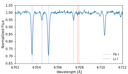
Figure 1: HIRES spectrum of TOI-1347 in the neighborhood of the lithium doublet. Nearby Fe I lines are labelled. No absorption attributed to lithium was detected.

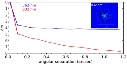
Figure 2: Contrast curves around TOI-1347 from Gemini/ ‘ Alopeke; the inset shows the reconstructed image at 832 nm. No companions are detected.

3 High Resolution Imaging

To help validate the transiting planets, we observed TOI-1347 with the ‘ Alopeke (Scott et al., 2021) dual-channel speckle imaging instrument on Gemini-N (PI: Crossfield) with a pixel scale of 0.01 arcsec/pixel and a full width at half maximum resolution of 0.02 arcsec. With ‘ Alopeke we obtained simultaneous speckle imaging at 562 and 832 nm, with a total of seven observing blocks each consisting of one thousand 60 ms exposures.

We processed these images with the speckle pipeline of Howell et al. (2011), which yielded the 5-sigma sensitivity curves and reconstructed image shown in Fig. 2. The curves do not show companions at angular separations of 0.5 arcsec or greater at a contrast of 4.12 mag at 562 nm and 6.52 mag at 832 nm (Fig. 2).

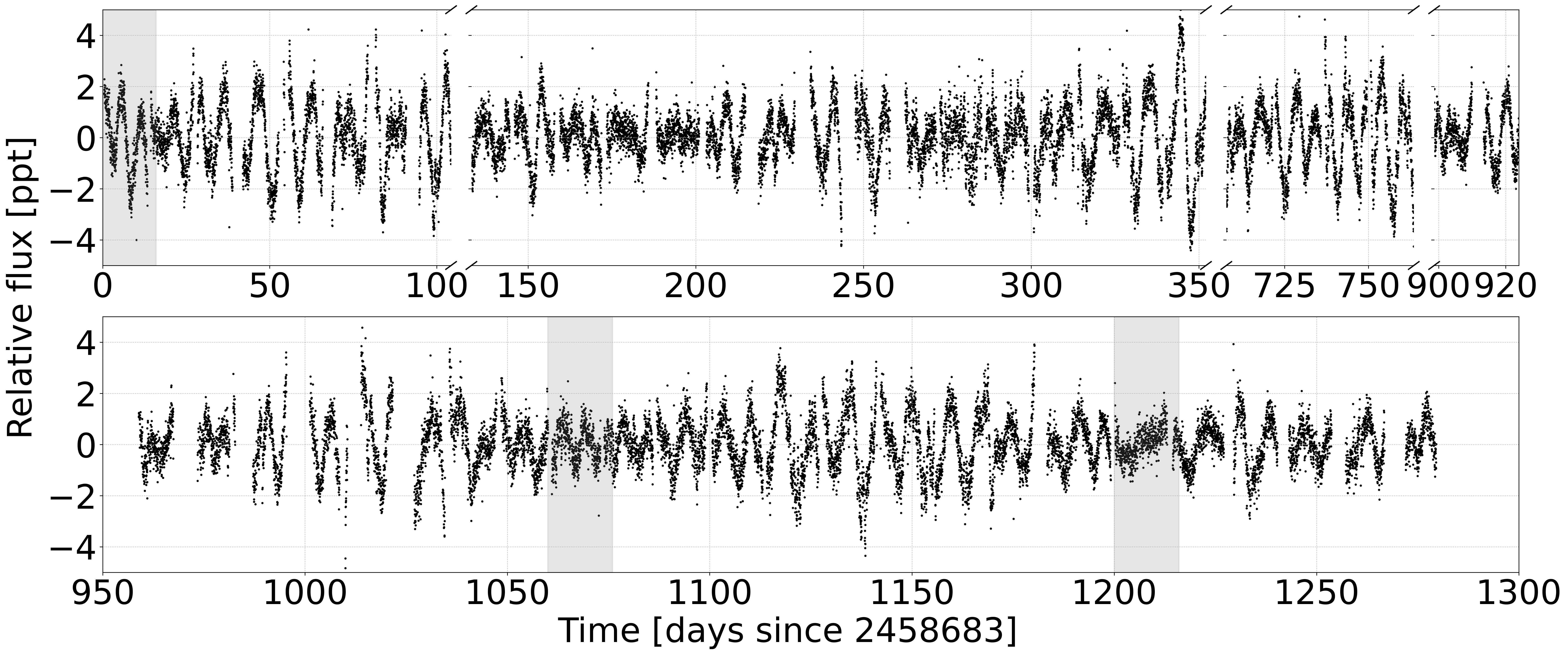
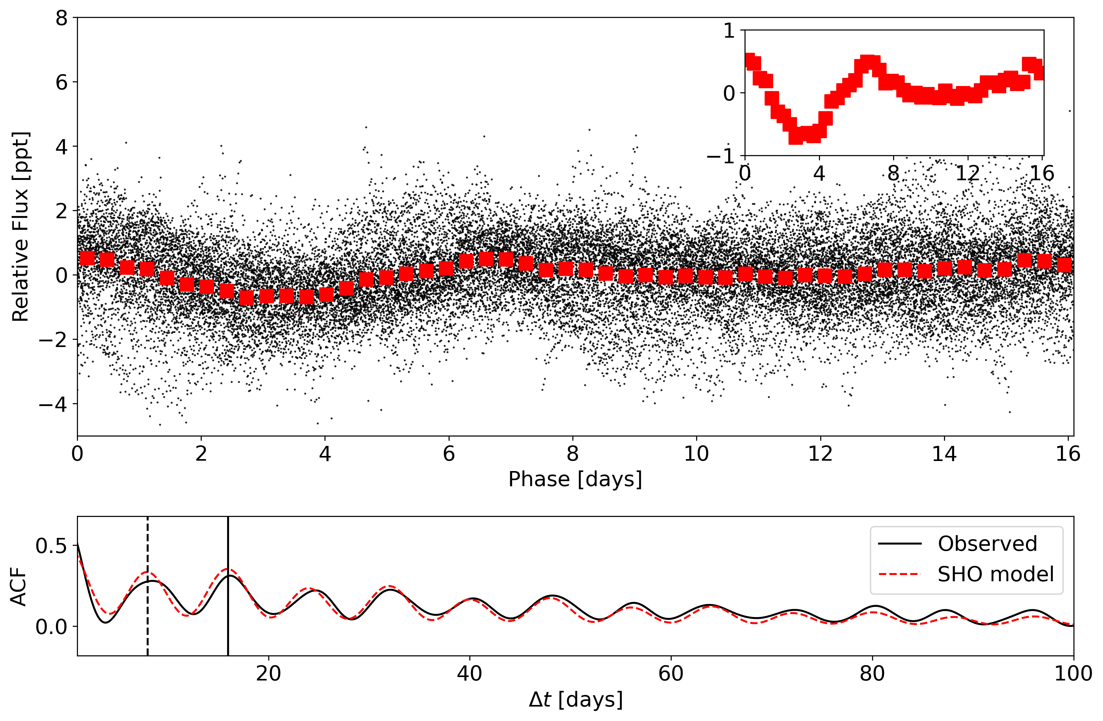
Figure 3: Top: The full 120 s cadence SPOC TESS light curve, binned to 30 min. Rotationally modulated variability is strong and evolves over time; the three shaded regions highlight example 16 day windows in which different numbers of maxima/minima are observed. Middle: The 30-min light curve phased to the 16.1 day rotation period. The red points further bin the folded data to $\sim 8$ hour bins. The inset zooms in on these binned phased data and highlights the tendency for every other set of maximum/minimum to repeat in amplitude. Bottom: The ACF of the photometry, showing regular peaks at all multiples of 8 days (dashed line) with the highest peak at 16 days (dark line). The red dashed line shows the best-fit SHO model described in Section 4.1.

Table 1: Stellar Parameters of TOI-1347

Parameter	Value	Unit	Source
TIC ID	TIC 229747848		TIC v8.2a
Right Ascension	18:41:18.4	hh:mm:ss	TIC v8.2a
Declination	+70:17:24.19	dd:mm:ss	TIC v8.2a
V magnitude	$11.168\pm 0.013$		TIC v8.2a
TESS magnitude	$10.7157\pm 0.0066$		TIC v8.2a
J magnitude	$10.011\pm 0.02$		TIC v8.2a
K magnitude	$9.616\pm 0.015$		TIC v8.2a
Gaia magnitude	$11.2076\pm 0.0005$		Gaia DR3b
Parallax	$6.7803\pm 0.0112$	mas	Gaia DR3b
RA proper motion	$-6.0883\pm 0.0150$	mas/yr	Gaia DR3b
Dec proper motion	$26.1020\pm 0.0150$	mas/yr	Gaia DR3b
Galactic U	$-5.31\pm 0.09$	km/s	Derived from Gaia DR3 astrometryc
Galactic V	$-7.72\pm 0.46$	km/s	Derived from Gaia DR3 astrometryc
Galactic W	$4.91\pm 0.23$	km/s	Derived from Gaia DR3 astrometryc
Luminosity	$0.55\pm 0.02$	$\text{L}_{\odot}$	Isoclassifyd
Radius	$0.83\pm 0.03$	$\text{R}_{\odot}$	Isoclassifyd
Mass	$0.913\pm 0.033$	$\text{M}_{\odot}$	SpecMatch-Synthetice
$T_{\text{eff}}$	$5464\pm 100$	K	SpecMatch-Synthetice
$\log{g}$	$4.64\pm 0.10$		SpecMatch-Synthetice
$[\mbox{Fe}/\mbox{H}]$	$0.04\pm 0.06$	dex	SpecMatch-Synthetice
$[\alpha/\text{Fe}]$	$-0.03\pm 0.06$	dex	KeckSpecf
$v\sin i_{\star}$	$<3$	km/s	SpecMatch-Synthetice
$v\sin i_{\star}$	$2.9\pm 0.1$	km/s	FASMAg
$v_{eq}$	$2.61\pm 0.11$	km/s	From $P_{\text{rot}}$ and $R_{\ast}$
$\log{R^{\prime}_{\mbox{\scriptsize HK}}}$	$-4.66\pm 0.05$		From Keck/HIRES spectrum
$P_{\text{rot}}$	$16.1\pm 0.3$	days	From ACF of TESS photometry (Section 4.1)
$P_{\text{rot}}$	$16.3\pm 0.6$	days	From TESS-SIP with TESS photometry (Section 4.1)
$P_{\text{rot}}$	$16.2\pm 0.3$	days	From GP fit to RVs (Section 5.1)
Age	$1.7\pm 0.1$	Gyr	From $P_{\text{rot}}$ using empirical relations of Bouma et al. (2023)
Age	$1.33\pm 0.06$	Gyr	From $P_{\text{rot}}$ using empirical relations of Mamajek & Hillenbrand (2008)
Age	$1.6\pm 0.4$	Gyr	From $\log{R^{\prime}_{\mbox{\scriptsize HK}}}$ using empirical relations of Mamajek & Hillenbrand (2008)
Age	$0.8_{-0.6}^{+1.1}$	Gyr	From isochronal fitting by MacDougall et al. (2023)
Age	$>650$	Myr	From Li and comparison to Hyades (Berger et al., 2018)
Age	$1.4\pm 0.4$	Gyr	Adopted value

4 TESS Photometry

TOI-1347 was observed by TESS in sectors 14–26, 40, 41, and 47–60, which span UT Jul 18 2019 to Jan 18 2023. The Science Processing Operations Center (SPOC; Jenkins et al., 2016) detected two transiting planet candidates which were subsequently diagnosed and vetted as TESS Objects of Interest (TOIs) 1347.01 (b) and 1347.02 (c) (Guerrero et al., 2021).

We downloaded the 20 s and 120 s cadence SPOC light curves using lightkurve (Lightkurve Collaboration et al., 2018). We removed all data points with a non-zero Quality Flag, i.e. those suffering from cosmic rays or other known systematic issues. We then stitched and normalized the multi-sector data using lightkurve and applied a 5-$\sigma$ sigma-clipping. lightkurve also provides the correction for scattered light (2% contamination reported by ExoFOP). The resulting light curve, shown in Figure 3, exhibits significant but coherent periodic variability corresponding to rotationally modulated surface inhomogeneities on the stellar disk.

4.1 Stellar Rotation Period

The effect of a starspot on photometry is to reduce the observed (integrated) intensity when on the visible hemisphere. The net effect of many spots is quasiperiodic variability that can be treated as time-correlated noise (Haywood et al., 2014; Rajpaul et al., 2015; Aigrain & Foreman-Mackey, 2023). The TESS photometry of TOI-1347 shows strong rotational variability with maxima/minima occurring roughly every $\sim 8$ days (see the top panel in Figure 3). A Lomb-Scargle periodogram of the photometry shows a strong peak at 8 days (Fig 4). However, a closer examination of the light curve reveals that the depths of adjacent maxima/minima are dissimilar. In fact, the depths of alternating maxima/minima tend to have similar amplitudes. This can be explained if the star has a 16 day rotation period and multiple spot groups concentrated on opposite hemispheres of the star, an effect noted for a number of other stars (Holcomb et al., 2022). In fact, a periodogram analysis of the RV dataset shows a strong peak at 16 days (Fig 4). Spots affect RVs in much the same way as photometry by breaking the flux balance across star’s rotational velocity profile (Saar & Donahue, 1997), in addition to suppressing the convective blueshift (Haywood et al., 2016).

While the periodogram is essentially a Fourier decomposition showing the amplitude of the best-fitting sine wave at all possible periods, the autocorrelation function (ACF) measures the self-similarity of a time series as a function of time delay. Thus, if the variability in a time series is not sinusoidal (asymmetric, more complex shape), then the ACF will give a better estimate of the periodicity than the periodogram. The ACF of the TESS photometry has its highest peak at $\sim$16 days (Fig 3) with adjacent ACF peaks alternating between high and low amplitude. An analysis of the ACF using spinspotter (Holcomb et al., 2022) successfully identified the half-period effect by checking that the odd peaks are less than 10% the height of the even peaks. spinspotter returns a rotation period of $P_{\text{rot}}=16.1\pm 0.3$ days by averaging the locations of the even-numbered peaks only. We also measured the stellar rotation period using the TESS Systematics Insensitive Periodogram algorithm (TESS-SIP Hedges et al., 2020). TESS-SIP simultaneously corrects for instrument systematics while performing the periodogram search on the TESS Simple Aperture Photometry. Using TESS-SIP for sectors 14-26 for TOI-1347, we measured a stellar rotation period of $16.34\pm 0.57$ days.

With all of this considered, we adopt the $\sim$16 day solution as the rotation period of TOI-1347 and explain the Lomb-Scargle periodogram peak at $P_{\text{rot}}/2$ as arising from antipodal spot groups. The persistence of repeated peaks every 8 days in the ACF, even out to beyond 100 days, can be explained if the starspots on TOI-1347 live for many rotation periods. Following the prescription of Giles et al. (2017), we fit the observed ACF with an underdamped simple harmonic oscillator (uSHO), including a second component with power at $P/2$:

$$y=e^{-\Delta t/\tau}\left[A\cos\left(\frac{2\pi\Delta t}{P}\right)+B\cos\left(\frac{2\pi\Delta t}{P/2}\right)+y_{0},\right].$$ (1)

In Eq. 1, $y$ is the ACF strength and the coefficients $A$ and $B$ give the relative strengths of the antipodal spot groups. We used scipy.optimize (Virtanen et al., 2020) to find the maximum a-posteriori (MAP) solution, then used that as a seed for a Markov-chain Monte Carlo (MCMC) analysis using emcee (Foreman-Mackey et al., 2013). The fit recovered $P=16.0$ d, and the best-fit exponential decay timescale was $\tau=45$ days, roughly three times the rotation period. Both coefficients $A=0.05$ and $B=0.18$ were constrained to nonzero values, again supporting the multiple spot group hypothesis.

Lastly, our SpecMatch-Synthetic analysis of the HIRES spectrum in Section 2.1 yielded only an upper limit corresponding to the line spread function of HIRES (roughly 2.2 km s^-1). Masuda et al. (2022) recently showed that on the population level, such nondetections of $v\sin i_{\star}$ are most consistent with a $<3$ km s^-1 upper-limit. Combining $P_{\text{rot}}=16.1$ d with the stellar radius from Section 2.1, we get an equatorial rotational velocity of $v_{eq}=2.6\pm 0.1$ km s^-1. This is consistent with a $<3$ km s^-1 upper-bound for HIRES, though it is slightly smaller than the measured HARPS-N value. Were the rotation period 8 d, we would instead have $v_{eq}\sim 5$ km s^-1, which (barring a misaligned stellar inclination of $\lesssim 30^{\circ}$) would be detectable in the HIRES spectrum and inconsistent with the HARPS-N measurement. If astrophysical, the slightly larger $v\sin i_{\star}$ could be explained by differential rotation and long-lived starspots at higher latitudes.

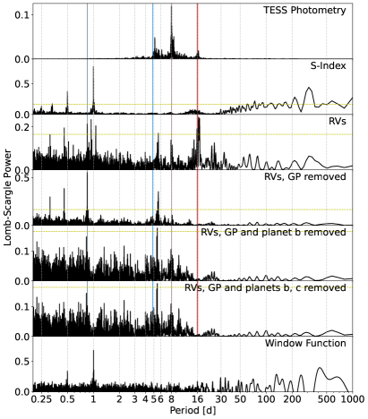
Figure 4: Lomb-Scargle periodograms of, from top to bottom, the TESS photometry, S-Indices, RVs, RVs with the GP model (Section 5.1) removed, the GP-corrected RVs with the Keplerian model for the USP subtracted, the GP-corrected RVs with both planets subtracted, and the window function (Dawson & Fabrycky, 2010) of the RV time series. The periodograms are computed using astropy.timeseries.LombScargle (Astropy Collaboration et al., 2022). The blue dashed lines correspond to the orbital periods of TOI-1347 b and c, and the two dark red lines are drawn at 8 days (thin) and 16 days (thick). The horizontal yellow line is the 1% false alarm probability.

4.2 Additional Transiting Planets?

We searched the TESS light curve for planetary transits with a Box-Least-Squares algorithm (BLS, Kovács et al., 2002) as described in Dai et al. (2021). We recovered the two planet candidates reported by ExoFOP at 0.84 and 4.84 days. We did not find any other transit signals with SNR $>6.5$.

4.3 Transit Modeling

Our transit analysis closely follows that described in (Dai et al., 2021). Briefly, we generated transit signals using the Python package Batman (Kreidberg, 2015), parameterized with the stellar density ($\rho_{\ast}$) to break the degeneracy between the scaled semimajor axes ($a/R_{\ast}$) and impact parameters ($b$) of the transiting planets (Seager & Mallén-Ornelas, 2003). We imposed a prior using the best-fit stellar density from our adopted $M_{\ast}$ and $R_{\ast}$ of $\rho_{\ast}=2.25\pm 0.26$ g cm^-3. For the limb darkening coefficients, we used the prior and parameterization scheme of Kipping (2013) for a quadratic limb darkening law ($q_{1}$ and $q_{2}$). The other transit parameters included the orbital period ($P_{\text{orb}}$), time of conjunction ($T_{\text{c}}$), planet-to-star radius ratios ($R_{\text{p}}/R_{\star}$), scaled orbital distances ($a/R_{\star}$, computed from stellar density and orbital period), orbital inclinations (cos$i$), orbital eccentricities ($e$), and the arguments of pericenter ($\omega$). We initially allowed non-zero eccentricities for both TOI-1347 b and c; however, the posterior distributions are fully consistent with circular orbits. Neither the existing transit nor RV data (Section 5) support the detection of nonzero eccentricities. In our final fits, we chose to restrict both planets to circular orbits to reduce model complexity.

Our transit fitting pipeline takes the following steps:

1. Fit a global model of all transit epochs, assuming no transit timing variations (TTVs). This model is found by maximizing the likelihood with the Levenberg-Marquardt method implemented in Python package lmfit (Newville et al., 2014).

2. Search for TTVs: We held the transit shape parameters fixed and fit for the mid-transit times of each transit epoch. We removed out-of-transit variations with a quadratic model. We did not detect significant TTVs for either planet, so we continued with fixed orbital periods.

3. Full model. We sampled the posterior distributions of both planets jointly using the MCMC framework implemented in emcee (Foreman-Mackey et al., 2013) with 128 walkers initialized near the MAP solution. We ran emcee for 50000 steps, ensuring that this was many times longer than the autocorrelation of various parameters (typically 100s of steps).

Fig. 5 shows the phase-folded and binned transits of TOI-1347 b and c with the MAP model. Using the stellar radius derived in Section 2, we derived $R_{p,b}=1.8\pm 0.1~{}\text{R}_{\oplus}$ and $R_{p,c}=1.6\pm 0.1~{}\text{R}_{\oplus}$, in agreement with the radii measured by MacDougall et al. (2023) ($R_{p,b}=1.81^{+0.09}_{-0.06}~{}\text{R}_{\oplus}$ and $R_{p,c}=1.68^{+0.09}_{-0.07}$).

Table 2: Transit and RV Parameters of the TOI-1347 System

Parameter	Symbol	Prior	Posterior Distribution	Unit
TOI-1347 b
Planet/Star Radius Ratio	$R_{p}/R_{\star}$	$\text{Uniform}(-10,10)$ on $\ln(R_{p}/R_{\star})$	$0.02039\pm 0.00072$
Time of Conjunction	$T_{c}$	$\text{Uniform}(1682,1683)$	$1682.71214\pm 0.00060$	(BJD-2457000)
Orbital Period	$P_{\text{orb}}$	Uniform(-10,10) on $\ln(P_{\text{orb}})$	$0.84742346\pm 0.00000061$	days
Orbital Inclination	$i_{\text{orb}}$	$\text{Uniform}(-1,1)$ on $\cos i_{\text{orb}}$	$79.5\pm 0.7$	deg
Orbital Eccentricity	$e$	-	0 (fixed)
Impact Parameter	$b$	Derived	$0.82\pm 0.03$
Scaled Semi-major Axis	$a/R_{\star}$	Derived	$4.43\pm 0.21$
RV Semi-amplitude	$K$	$\text{Normal}(0,50)$	$7.74^{+0.80}_{-0.79}$	m s-1
Planetary Radius	$R_{\rm p}$	Derived	$1.8\pm 0.1$	$\text{R}_{\oplus}$
Planetary Mass	$M_{\rm p}$	Derived	$11.1\pm 1.2$	$\text{M}_{\oplus}$
Bulk Density	$\rho$	Derived	$9.9_{-1.7}^{+2.1}$	g cm-3
Equilibrium Temperature	$T_{\rm eq}$	Derived ($A_{B}=0.7$)	$1400\pm 40$	K
TOI-1347 c
Planet/Star Radius Ratio	$R_{p}/R_{\star}$	$\text{Uniform}(-10,10)$ on $\ln(R_{p}/R_{\star})$	$0.0179\pm 0.0010$
Time of Conjunction	$T_{c}$	$\text{Uniform}(1678,1679)$	$1678.5059\pm 0.0021$	(BJD-2457000)
Orbital Period	$P_{\text{orb}}$	$\text{Uniform}(-10,10)$ on $\ln(P_{\text{orb}})$	$4.841962\pm 0.000012$	days
Orbital Inclination	$i$	$\text{Uniform}(-1,1)$ on $\cos i_{\text{orb}}$	$87.5\pm 0.4$	deg
Orbital Eccentricity	$e$	-	0 (fixed)
Impact Parameter	$b$	Derived	$0.73\pm 0.08$
Scaled Semi-major Axis	$a/R_{\star}$	Derived	$14.18\pm 0.49$
RV Semi-amplitude	$K$	$\text{Normal}(0,50)$	$1.08^{+0.91}_{-0.92}~{}(<2.59~{}\text{at 95\%})$	m s-1
Planetary Radius	$R_{\rm p}$	Derived	$1.6\pm 0.1$	$\text{R}_{\oplus}$
Planetary Mass	$M_{\rm p}$	Derived	$2.8\pm 2.3~{}(<6.4~{}\text{at 95\%})$	$\text{M}_{\oplus}$
Bulk Density	$\rho$	Derived	$3.6_{-3.0}^{+3.3}~{}(<4.1~{}\text{at 95\%})$	g cm-3
Equilibrium Temperature	$T_{\rm eq}$	Derived ($A_{B}=0.1$)	$1000\pm 25$	K
Stellar Parameters
Stellar Density	$\rho_{\star}$	$\text{Normal}(2.25,0.26)$	$2.30\pm 0.24$	g cm-3
Limb Darkening	$q_{1}$	$\text{Uniform}(0,1)$	$0.28\pm 0.20$
Limb Darkening	$q_{2}$	$\text{Uniform}(0,1)$	$0.35\pm 0.28$
HIRES RV Jitter	$\sigma_{\rm HIRES}$	$\text{HalfNormal}(0,10)$	$4.05^{+0.73}_{-0.67}$	m s-1
HARPS-N RV Jitter	$\sigma_{\rm HARPS}$	$\text{HalfNormal}(0,10)$	$8.20^{+2.67}_{-1.98}$	m s-1
GP Amplitude	$A_{\text{GP}}$	InverseGamma(1, 5)	$9.70^{+1.16}_{-1.06}$	m s-1
Rotation Period	$P_{\text{GP}}$	$\text{Normal}(\ln(16),0.5)$ on $\ln(P_{\text{GP}})$	$16.16^{+0.35}_{-0.35}$	days
Oscillator Quality Factor	$Q_{0}$	$\text{HalfNormal}(0,2)$ on $\ln(Q_{0})$	$1.49^{+0.74}_{-0.91}$
Quality Factor Difference	$\Delta Q$	$\text{Normal}(0,2)$ on $\ln(\Delta Q)$	$1.71^{+1.32}_{-2.33}$
Fractional Amplitude	$f$	$\text{Uniform}(0.1,1)$	$0.73^{+0.19}_{-0.24}$
Instrumental RV Parameters
RV Offset (HIRES)	$\gamma_{\rm HIRES}$	$\text{Normal}(0,200)$	$-2.12^{+0.90}_{-0.87}$	m s-1
RV Offset (HARPS-N)	$\gamma_{\rm HARPS}$	$\text{Normal}(0,200)$	$6.29^{+3.35}_{-3.41}$	m s-1

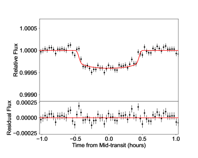
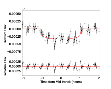
Figure 5: The 2 min TESS light curves phase-folded and binned using the orbital periods of TOI-1347 b (top) and c (bottom). The best-fit transit models are shown with red solid lines.

4.4 Phase Curve

We searched the TESS light curve for phase curve variations and secondary eclipses of TOI-1347 b. First, we masked the in-transit data and removed long-term variability (stellar and/or instrumental) using the method of Sanchis-Ojeda et al. (2013). This involves fitting a linear function of time to the out-of-transit data points within a window of 2$\times$ the orbital period, then dividing the best-fit function within that window, repeating for every data point in the light curve. This detrended light curve is then phase-folded to the orbital period of TOI-1347 b.

The resultant phase curve is shown in Figure 6. We were able to detect a tentative phase curve variation (3$\sigma$) and a secondary eclipse (2$\sigma$) using a joint model. To model the secondary eclipse, we simply modified the best-fit transit model by shifting the mid-transit times by half the orbital period (i.e., assuming $e=0$) and turning off limb darkening ($q_{1}$ = $q_{2}$ = 0). The secondary eclipse depth ($\delta_{\rm sec}$) is allowed to vary freely to account for a combined effect of reflected stellar light and thermal emission from the planet’s night side. For the phase curve, we used a Lambertian disk model (see e.g. Demory et al., 2016) parameterized by an amplitude $A$ and phase offset of the peak $\theta$. We sampled the posterior distribution with a MCMC analysis similar to that described in Section 4.3. We found a secondary eclipse depth of $\delta_{\rm sec}=26\pm 12$ ppm and a phase curve amplitude of $A=28\pm 9$ ppm. The peak of the phase curve variation is shifted by $33\pm 14^{\circ}$ to the west of the planet.

The lower panel of Figure 6 compares the amount of thermal emission vs. reflected light as a function of the planet’s Bond albedo ($A_{B}$). At high albedo, the planet is more reflective and the equilibrium temperature will be lower. In this case, the phase curve will be dominated by reflected stellar light rather than thermal emission. This is necessary to explain the large secondary eclipse depth measured in the TESS band. Moreover, we marginally detected a phase offset of $33\pm 14^{\circ}$ to the west of the planet. Both of these effects can be explained if TOI-1347 b is retaining a high-mean-molecular-weight atmosphere. Silicate clouds in this atmosphere could produce a high albedo, while partial cloud coverage may produce the observed phase offset to the West (see e.g. Kepler-7 b, Demory et al., 2013). However, the data in hand are insufficient to definitively confirm the presence of an atmosphere on TOI-1347 b. Higher SNR follow-up observations with JWST are required.

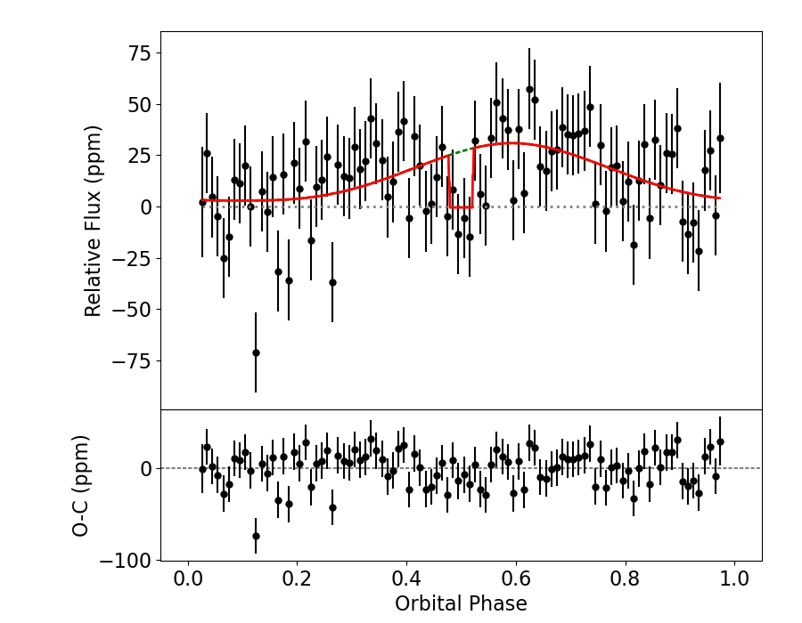
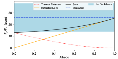
Figure 6: Upper: The phase curve and secondary eclipse of TOI-1347 b as observed by TESS. The best-fit model is shown by the red curve. The green dotted line gives the model with no eclipse. The phase curve is detected at the 2$\sigma$ level. It is likely a combination of thermal emission and reflected light in the TESS band (600–1000 nm). Lower: The thermal emission (red dotted line) and reflected light (orange solid line) from TOI-1347 b as a function of the Bond albedo. The blue dashed line and shaded area are the measured secondary eclipse depth ($F_{p}/F_{\star}$) and its 1$\sigma$ central interval.

5 Radial Velocities

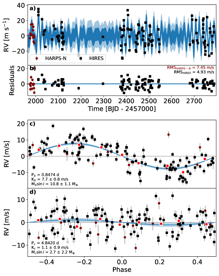
Figure 7: The adopted radial velocity model. Panel a) shows the HARPS-N and HIRES RV datasets, with the MAP RV model (Keplerian + GP and 1$\sigma$ uncertainty) overplotted in blue. Panel b) shows the residuals between the data and the MAP RV model. Panels c) and d) show the data phase-folded to the orbital period of planets b and c, respectively, with contributions from the other planet and the GP removed. The red points are equal RV bins spanning 0.1 in phase. The median and central 68% CI of each Keplerian model is plotted in blue. The MCMC posteriors for the recovered semiamplitude and derived $M\sin i$ are also summarized in the lower-left annotations. Note that we do not include the MAP stellar jitter in the plotted errorbars; errorbars are drawn only as the measurement uncertainties to highlight the degree of unexplained scatter (i.e., jitter), given by the annotated residual RMS, to which the stellar jitter fits.

We collected 120 high-resolution optical spectra of TOI-1347 between UT November 28, 2019 and UT July 26, 2022 with HIRES on the Keck-I telescope as part of TKS (Chontos et al., 2022). We took exposures using the “C2” decker ($R=45,000$) and integrated until the exposure meter reached 60,000 counts (signal-to-noise ratio (S/N) $\sim 100$ per reduced pixel) which resulted in a typical exposure time of 648 sec. We used the standard procedures of the California Planet Search (CPS; Howard et al., 2010) to reduce the HIRES spectra and extract precise RVs using the iodine cell for wavelength calibration (Butler et al., 1996). The average Doppler precision per measurement was 1.83 m s^-1.

We also obtained 14 spectra with the High-Accuracy Radial-velocity Planet Searcher in the North, installed at the Telescopio Nazionale Galileo (HARPS-N; Cosentino et al., 2012). Observations were taken with 1800 s exposure times (average S/N is 42.3 in order 50) with simultaneous wavelength calibration provided by the Fabry-Perot etalon. Cross-correlation functions (CCFs) were created using the ESPRESSO G2 mask, and RVs were extracted by fitting for the CCF centroid (Dumusque et al., 2021). Before jointly fitting with the HIRES RVs, we subtracted the median RV from the HARPS-N dataset.

See Table 3 for the full RV dataset, which includes Mount Wilson S-Index values derived from the Ca II H& K lines (Duncan et al., 1991) for the HIRES data. The $S_{\mathrm{HK}}$ index shows a weaker power excess around $P_{\text{rot}}$ in a Lomb-Scargle periodogram than the RVs (Fig. 4) but are primarily dominated by a 1 day sampling alias. The $S_{\mathrm{HK}}$ indices are correlated with the RVs at the 3.5$\sigma$ level with a Pearson correlation coefficient of 0.31 (p-value of 0.0005). This weak correlation is likely why our models in Section 5.1 that were trained on the S-Index time series did not improve the overall fit.

5.1 RV Model

We chose to adopt the same two-component SHO model for our RV model that we used to model stellar variability in photometry. We used the exoplanet (Foreman-Mackey et al., 2021) package to construct a Gaussian Process (GP) stellar activity model with a kernel defined by the built-in RotationTerm parameterization. This kernel is a mixture of two SHOs analogous to the first and second cosine terms in Eq. 1. We also tried a GP with the quasiperiodic kernel implemented in radvel (Fulton et al., 2018), both untrained and trained on the S-Indices. We found that the quasiperiodic kernel struggled to identify a single primary period, often jumping between 8 days and 16 days. In order for the MCMC to converge, a reasonably strong prior ($\pm 0.5$ d or less) had to be placed on one of these period solutions. We found this undesirable compared to the SHO kernel in exoplanet, which was able to lock onto the 16 day period even with wide priors of $>10$ d. We also found the final fit to be statistically indistinguishable whether the GP was trained on the S-Indices or not, so for our final model we opted for an untrained SHO GP.

For the full mathematical definition of the SHO GP kernel, the interested reader is directed to Foreman-Mackey et al. (2017). In brief, the kernel is parameterized by the GP amplitude ($A_{\text{GP}}$), the primary period of variability ($P_{\text{GP}}$), the quality factor of the primary mode $Q_{0}$, the difference in quality factors between the period and half-period modes ($\Delta Q_{0}$), and lastly the fractional amplitude between the two modes ($f$). We followed the guidance of the exoplanet tutorials to choose the appropriate priors on these parameters, which are tabulated in Table 2.

In practice, the Keplerian models are only parameterized by the RV semiamplitude $K$, which we place a wide uninformative Gaussian prior on. We do not restrict $K$ to positive values only, as such a prior can bias mass estimates to higher values, especially in the case of non-detections (Weiss & Marcy, 2014). We imposed Gaussian priors on the periods and times of conjunction using the best-fit mean and standard deviation derived from our transit fits (Table 2), effectively fixing them to the tight transit constraints. Like the transit model, we fixed the eccentricity ($e$) and argument of periastron ($\omega$) to zero. We included separate jitter terms for HIRES ($\sigma_{\text{HIRES}}$) and HARPS-N ($\sigma_{\text{HARPS}}$), and likewise separate RV offsets ($\gamma_{\text{HIRES}}$) and HARPS-N ($\gamma_{\text{HARPS}}$).

We initialized our model at the best-fit values from photometry, where applicable, and determined initial guesses for the RV semiamplitudes using exoplanet.estimate_semi_amplitude. We then solved for the MAP solution using scipy.optimize.minimize. The MAP parameters were then used as a seed for a MCMC exploration of the posterior. We employed a Hamiltonian Monte Carlo (HMC; Duane et al., 1987; Neal, 2012) implemented in PyMC3 (Salvatier et al., 2016), specifically the No-U-Turn Sampler (NUTS; Hoffman & Gelman, 2014). HMC and NUTS are generally more efficient than the traditional Metropolis-Hatings algorithm (Metropolis et al., 1953; Hastings, 1970), resulting in well-mixed MCMC chains in far fewer samples. We sampled with NUTS in four parallel chains for 5000 “tuning” steps, which are discarded. The number of tuning steps was chosen to obtain an acceptance fraction near the target of 0.9 which balances number of retained samples and efficient exploration of the posterior space. Each chain then collects 5000 samples for a total of 20000 posterior samples. We ensured adequate statistical independence amongst these samples by requiring that the per-parameter $\hat{R}$ statistic (Vehtari et al., 2021) be $<1.001$.

Our best-fitting RV model is shown in Figure 7. The GP robustly recovers a primary period of $16.2\pm 0.3$ days, even with a wide prior, independently verifying our assessment of the stellar rotation period from photometry. The USP TOI-1347 b is also robustly detected at consistent semiamplitudes, regardless of the activity model used (trained/untrained, quasi-periodic/SHO). The resulting mass of TOI-1347 b is $11.1\pm 1.2~{}\text{M}_{\oplus}$. The second planet, TOI-1347 c, is not detected in the RVs. We adopt an upper limit of $<6.4~{}\text{M}_{\oplus}$ at 95% confidence. The residual RMS to the combined Keplerian + GP model is $4.9$ m s^-1 for HIRES and $7.5$ m s^-1 for HARPS-N, which is (expectedly) similar to the fitted stellar jitter values ($4.0\pm 0.7$ m s^-1 and $8.2_{-2.0}^{+2.7}$ m s^-1 respectively), but larger than the per-measurement uncertainty of each instrument (2.5 and 1.9 m s^-1).

Of note is the large jitter for the HARPS-N RVs. We suspect this is due to the GP being primarily conditioned on the HIRES RVs, resulting in poor predictive accuracy for activity during the timespan of the HARPS-N data, which occur about 1–2 rotation cycles before the HIRES data. As a result, the jitter term for HARPS-N is inflated to compensate. We tried separate GPs for both datasets, sharing all hyperparameters except for the GP amplitude ($A_{\text{GP}}$). We found a nearly identical result (in fact, the best-fit HARPS-N jitter was higher) with statistically indistinguishable planet parameters, likely due to the relatively few HARPS-N data points. As a result, we adopt the single GP model, but encourage further investigation into the nature of stellar activity on TOI-1347. As it stands, there are too few HARPS-N data points to condition independent GPs, but the single GP model is potentially overfitted to the HIRES points, reducing its out-of-sample predictive accuracy (Blunt et al., 2023).

6 Discussion

6.1 A Heavy Core Pushing the Limit of Photoevaporation

TOI-1347 b is the largest (in both mass and radius) of the super-Earth USPs to date. It seems to be rocky in composition and similar in iron core mass fraction to the Earth. Figure 8 shows the two planets in the context of known exoplanets on the mass-radius diagram. We modeled the core composition of TOI-1347 b assuming a simple two-layer model with an iron core and a silicate (“rock”) mantle (Zeng et al., 2016). Our mass and radius measurements suggest an iron core mass fraction of 41$\pm$ 27%, not far from Earth’s 33% core mass fraction. TOI-1347 b joins a group of well-characterized USP planets (Dai et al., 2019) that are consistent with an Earth-like composition.

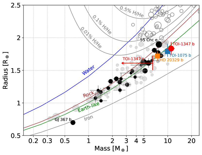
Figure 8: Mass-radius diagram of known super-Earths ($R_{p}<2~{}\text{R}_{\oplus}$, filled circles) and sub-Neptunes ($4~{}\text{R}_{\oplus}>R_{p}\geq 2~{}\text{R}_{\oplus}$, empty circles) with 5$\sigma$ or better mass measurements, obtained from the NASA Exoplanet Archive (NASA Exoplanet Archive, 2019). Bold fill denotes USPs. Contours from Zeng et al. (2016) are drawn for pure-iron, Earth-like (30% iron, 70% rock), pure-rock, and pure-water compositions. Contours from Chen & Rogers (2016) are also drawn for 0.5%, 0.1%, and 0.01% H/He envelopes surrounding rocky-composition cores, at an age of 1.4-Gyr-old and at the maximum insolation flux of 400 S_⊕ for their model grids; it is worth noting that TOI 1347 b (1400 K, $A=0.7$) receives an insolation flux of around 3000 S_⊕. Our mass-radius constraints for TOI-1347 b and c (95% upper limit in mass) are plotted and labelled in red. The size of each point is proportional to $M/\sigma_{M}$. TOI-1347 b is the most massive super-Earth USP to date, while TOI-1347 c is smaller but likely also rocky.

With a core mass larger than 10 $\text{M}_{\oplus}$, TOI-1347 b, along with the USPs TOI-1075 b (Essack et al., 2023), and HD 20329 b (Murgas et al., 2022), are close to the theoretical limit for runaway accretion (see, e.g., Rafikov, 2006). How did these planets evade runaway accretion and not become gas giants? Lee (2019) and Chachan et al. (2021) both noted that the local hydrodynamic conditions, the envelope opacity, and the timescale of core assembly relative to disk dissipation could all contribute to quenching runaway accretion. As more of these systems are discovered, population-level analyses may shed light on which planets are able to evade runaway and which grow into gas giants.

TOI-1347 b also pushes the efficacy of photoevaporation to its limit. At $>10~{}\text{M}_{\oplus}$, the outflowing atmosphere has to overcome a deep gravitational potential well. On the other hand, the temperature of atmospheric outflows is likely capped below $10^{4}$ K due to strong radiative cooling at higher temperatures (see, e.g., Murray-Clay et al., 2009). An order of magnitude comparison reveals that the thermal sound speed ($\sim$10 km s^-1 at $10^{4}$ K) may not overcome the escape velocity of the planet ($\sim$25 km s^-1 at $10~{}\text{M}_{\oplus}$ and $1.9~{}\text{R}_{\oplus}$), preventing bulk hydrodynamic outflow (i.e. photoevaporation). Previous models showed that photoevaporation is significantly quenched on planets with heavier cores ($\gtrsim 6~{}\text{M}_{\oplus}$, see e.g. Owen & Wu, 2017; Wang & Dai, 2018). Planets like TOI-1347 b are therefore important test cases to understand the limit of both photoevaporation and core-powered mass loss (Ginzburg et al., 2018; Gupta & Schlichting, 2019). Our mass and radius measurements disfavor the presence of a thick H/He envelope (Fig. 8). Did TOI-1347 b have, and then lose, a primordial H/He envelope? Or, could TOI-1347 b have formed near to its present-day scorching orbit without ever acquiring a substantial atmosphere? We encourage further investigation on this question.

6.2 A Heavy-Mean-Molecular-Weight Atmosphere?

Even though TOI-1347 b has a mass and radius that suggest an Earth-like bulk composition, we cannot rule out the presence of a heavy-mean-molecular-weight atmosphere. Lopez (2017) showed that the largest of the non-giant USPs (such as 55 Cnc e) can hold onto high-metallicity atmospheres even in the presence of strong stellar radiation. Such an atmosphere would only marginally inflate the planet’s radius (the scale height of a CO₂ based atmosphere is about 11 km, while planetary radii are  $\sim$10,000 km).

In fact, our tentative phase curve (3$\sigma$) and secondary eclipse (2$\sigma$) detections of TOI-1347 b point to a nonzero albedo and a possible phase offset to the west. These features could indicate the presence of an atmosphere at least partially covered by reflective silicate clouds. It may be the case that the deep gravitational wells of the most massive super-Earth USPs are sufficient to cling to such an atmosphere and resist atmospheric loss mechanisms. Hu et al. (in prep.) show that their JWST NIRCam and MIRI observations of 55 Cnc e, a similar massive USP (0.73-day orbit; 9$M_{\oplus}$), can only be explained if the planet still has a CO or CO₂ based atmosphere. Future observations with JWST might uncover a similar story for TOI-1347 b (TSM$=19$, ESM$=5.6$, using the equations of Kempton et al. 2018).

Alternatively, the high-amplitude TESS phase curve of TOI-1347 b may be a consequence of outgassed Na emission on the hot dayside of the planet. Zieba et al. (2022) showed that this emission can explain the phase curve of the lava world K2-141 b, which has been observed in both the Kepler passband and Spitzer-4.5 $\mu$m passband (Malavolta et al., 2018). In their analysis, they found that the two phase curves are inconsistent with a blackbody model, with the visible-light phase curve having a higher amplitude than expected. Similarly high visible-light phase curve amplitudes have been reported for the lava worlds 55 Cnc e (Kipping & Jansen, 2020) and Kepler-10 b (Batalha et al., 2011; Rouan et al., 2011), although the latter has not yet been observed in the infrared, which would test blackbody emission. If Na emission is responsible for the observations of TOI-1347 b reported here, it may more easily explain the tentative phase curve offset than reflective clouds, which would need to be nonuniformly distributed across the planet.

7 Summary

We have characterized two transiting planets in the TOI-1347 system, TOI-1347 b, a USP (0.85 d), and its outer small companion TOI-1347 c (4.84 d). Using TESS photometry and an independent transit fitting pipeline, we measured a radius of $1.8\pm 0.1~{}\text{R}_{\oplus}$ for the USP, and $1.6\pm 0.1~{}\text{R}_{\oplus}$ for its companion. We conducted a RV campaign of the TOI-1347 system with HIRES (as part of TKS) and with HARPS-N. We measured a mass of $11.1\pm 1.2~{}\text{M}_{\oplus}$ for the USP, consistent with a bulk Earth-like composition and inconsistent with a H/He envelope (see Fig 8). This composition is perhaps unsurprising given the system age of $1.4\pm 0.4$ Gyr, the short timescale on which intensive photoevaporation operates (few 100 Myr), and the high insolation flux at TOI 1347 b’s orbit; any primordial H/He envelope should have been destroyed by now. We were unable to detect the companion TOI-1347 c with RVs. We placed a 95% upper limit of $<6.4~{}\text{M}_{\oplus}$. Of note is the minimum mutual inclination between planets b and c implied by our measured orbital inclinations: $\sim 7^{\circ}$. This is unusually large compared to typical Kepler multis (Fabrycky et al., 2014), which may be another indicator of the migration dynamics that produce USPs.

TOI-1347 b is the most massive of the $<2~{}\text{R}_{\oplus}$ (i.e., primarily solid by volume) USPs to date. Its mass sets an upper limit on runaway accretion processes and places TOI-1347 b in a region of the mass-radius diagram in which the pressures and temperatures reached inside the planet have not been well characterized either by experiments or theoretical modeling.

Intriguingly, we measured a tentative (3$\sigma$) phase-curve variability, as well as a secondary eclipse (2$\sigma$) for the USP TOI-1347 b. The phase curve asymmetry strongly suggests an optically thick atmosphere. However, our mass and radius measurements of TOI-1347 b are highly inconsistent with any significant H/He envelope. As a result, any such atmosphere must have a high mean molecular weight. It could be comprised of reflective silicate clouds, or may be the result of the outgassing of Na from the molten surface. Future observations (e.g. with JWST) would help confirm such an atmosphere and reveal its composition.

8 Acknowledgements

Some of the data presented herein were obtained at the W. M. Keck Observatory, which is operated as a scientific partnership among the California Institute of Technology, the University of California, and the National Aeronautics and Space Administration. The Observatory was made possible by the generous financial support of the W. M. Keck Foundation. Keck Observatory occupies the summit of Maunakea, a place of significant ecological, cultural, and spiritual importance within the indigenous Hawaiian community. We understand and embrace our accountability to Maunakea and the indigenous Hawaiian community, and commit to our role in long-term mutual stewardship. We are most fortunate to have the opportunity to conduct observations from Maunakea.

This paper made use of data collected by the TESS mission and are publicly available from the Mikulski Archive for Space Telescopes (MAST) operated by the Space Telescope Science Institute (STScI). All the TIC data used in this paper can be found in MAST: http://dx.doi.org/10.17909/fwdt-2x66 (catalog 10.17909/fwdt-2x66) (STScI, 2018). All the TESS data used in this paper can be found in MAST: http://dx.doi.org/t9-nmc8-f686 (catalog 10.17909/t9-nmc8-f686) (MAST, 2021). Data from the NASA Exoplanet Archive can be found at http://dx.doi.org/10.26133/NEA1 (catalog 10.26133/NEA1) (NASA Exoplanet Archive, 2019). Funding for the TESS mission is provided by NASA’s Science Mission Directorate. We acknowledge the use of public TESS data from pipelines at the TESS Science Office and at the TESS Science Processing Operations Center. This work is based also on observations made with the Italian Telescopio Nazionale Galileo (TNG) operated on the island of La Palma by the Fundación Galileo Galilei of the INAF (Istituto Nazionale di Astrofisica) at the Spanish Observatorio del Roque de los Muchachos of the Instituto de Astrofisica de Canarias. Some of the observations in this paper made use of the High-Resolution Imaging instrument ‘ Alopeke. ‘ Alopeke was funded by the NASA Exoplanet Exploration Program and built at the NASA Ames Research Center by Steve B. Howell, Nic Scott, Elliott P. Horch, and Emmett Quigley. ‘ Alopeke was mounted on the Gemini North telescope of the international Gemini Observatory, a program of NSF’s NOIRLab, which is managed by the Association of Universities for Research in Astronomy (AURA) under a cooperative agreement with the National Science Foundation.

We thank the time assignment committees of the University of California, the California Institute of Technology, NASA, and the University of Hawaii for supporting the TESS-Keck Survey with observing time at Keck Observatory and on the Automated Planet Finder. We thank NASA for funding associated with our Key Strategic Mission Support project. We gratefully acknowledge the efforts and dedication of the Keck Observatory staff for support of HIRES and remote observing.

R.A.R. acknowledges support from the National Science Foundation through the Graduate Research Fellowship Program (DGE 1745301). M.R. acknowledges support from Heising-Simons grant #2023-4478. D.H. acknowledges support from the Alfred P. Sloan Foundation, the National Aeronautics and Space Administration (80NSSC21K0652) and the Australian Research Council (FT200100871).

Keck-I: HIRES (Vogt et al., 1994), HARPS-N (Cosentino et al., 2012), TESS (Ricker et al., 2015), Gemini North: ‘ Alopeke (Scott et al., 2021)

Here we present the posterior distributions for the full RV model (Figure 9), as well as the table of RV observations analyzed in Section 5 (Table 3).

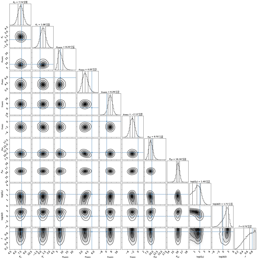
Figure 9: Full posterior distributions for the RV model described in Section 5.1. The blue lines denote the MAP values.

Table 3: TOI-1347 RVs and S-Indices

Time	RV	RV Error	$S_{\mathrm{HK}}$ Index	$S_{\mathrm{HK}}$ Index Error	Instrument
(BJD-2457000)	(m/s)	(m/s)
2458974.658616	-2.385	2.91	–	–	HARPS-N
2458976.56778	3.675	2.77	–	–	HARPS-N
2458977.647243	1.645	2.3	–	–	HARPS-N
2458978.664451	1.735	1.84	–	–	HARPS-N
2458979.661071	15.635	2.56	–	–	HARPS-N
2458983.624618	2.145	2.92	–	–	HARPS-N
2458985.688595	15.945	2.17	–	–	HARPS-N
2458987.721405	8.195	2.07	–	–	HARPS-N
2458988.675995	-1.315	1.57	–	–	HARPS-N
2458989.689122	12.705	2.12	–	–	HARPS-N
2458990.665386	-6.745	1.76	–	–	HARPS-N
2458991.669197	1.215	3.26	–	–	HARPS-N
2458992.622382	-1.215	4.22	–	–	HARPS-N
2458993.586943	-8.595	2.12	–	–	HARPS-N
2459011.871925	27.023	1.73	0.291	0.001	HIRES
2459011.945652	31.576	1.75	0.285	0.001	HIRES
2459011.999298	35.149	1.85	0.287	0.001	HIRES
2459028.000963	21.648	1.49	0.285	0.001	HIRES
2459034.871693	1.685	1.74	0.284	0.001	HIRES
2459036.801673	5.49	1.85	0.281	0.001	HIRES
2459040.959633	7.374	1.88	0.277	0.001	HIRES
2459043.067716	-14.481	1.69	0.278	0.001	HIRES
2459073.019955	-4.758	1.77	0.263	0.001	HIRES
2459079.02133	13.265	1.94	0.271	0.001	HIRES
2459086.759188	8.866	2.45	0.261	0.001	HIRES
2459094.963738	-0.889	1.81	0.256	0.001	HIRES
2459099.906082	-3.443	2.08	0.258	0.001	HIRES
2459101.74781	-6.744	1.72	0.275	0.001	HIRES
2459102.001018	0.082	1.95	0.274	0.001	HIRES
2459114.730454	17.792	1.68	0.277	0.001	HIRES
2459114.919621	11.108	1.97	0.277	0.001	HIRES
2459115.767787	4.19	1.76	0.281	0.001	HIRES
2459115.851596	-2.33	1.81	0.278	0.001	HIRES
2459117.73074	-17.608	1.7	0.276	0.001	HIRES
2459117.892083	-8.786	1.65	0.274	0.001	HIRES
2459118.725156	-2.82	1.71	0.275	0.001	HIRES
2459119.822351	3.015	1.62	0.262	0.001	HIRES
2459120.849961	-0.745	1.84	0.261	0.001	HIRES
2459121.893938	-10.875	1.62	0.263	0.001	HIRES
2459122.813237	-8.108	1.67	0.264	0.001	HIRES
2459123.723648	-7.533	1.58	0.264	0.001	HIRES
2459189.746637	-25.975	2.66	0.279	0.001	HIRES
2459297.143477	-1.254	2.29	0.319	0.001	HIRES
2459373.951805	9.778	1.68	0.306	0.001	HIRES
2459377.047988	-12.886	1.79	0.296	0.001	HIRES
2459377.869358	-18.981	1.72	0.296	0.001	HIRES
2459379.121054	7.817	1.65	0.29	0.001	HIRES
2459379.945803	-1.632	1.65	0.282	0.001	HIRES
2459382.038048	-28.729	2.01	0.268	0.001	HIRES
2459382.957833	-29.687	1.89	0.278	0.001	HIRES
2459385.051386	0.288	1.78	0.285	0.001	HIRES
2459385.877791	7.743	1.73	0.289	0.001	HIRES
2459388.847531	8.234	1.79	0.309	0.001	HIRES
2459389.113887	20.363	1.85	0.313	0.001	HIRES
2459389.840061	12.641	1.64	0.311	0.001	HIRES
2459390.10277	7.56	1.79	0.31	0.001	HIRES
2459396.049221	-11.462	1.87	0.281	0.001	HIRES
2459405.116336	8.808	1.68	0.309	0.001	HIRES
2459405.952026	9.326	1.77	0.315	0.001	HIRES
2459406.101749	33.565	1.79	0.31	0.001	HIRES
2459407.905698	27.179	1.8	0.0	0.001	HIRES
2459413.001295	8.237	1.94	0.284	0.001	HIRES
2459413.964231	-1.111	1.9	0.278	0.001	HIRES
2459414.118005	-18.948	2.63	0.239	0.001	HIRES
2459420.770145	8.008	1.68	0.292	0.001	HIRES
2459441.889385	-8.624	1.95	0.311	0.001	HIRES
2459442.029629	-18.863	1.85	0.305	0.001	HIRES
2459443.913165	-20.67	1.83	0.302	0.001	HIRES
2459446.031598	0.282	1.75	0.283	0.001	HIRES
2459448.761484	-3.308	2.23	0.281	0.001	HIRES
2459449.003801	-10.891	2.09	0.277	0.001	HIRES
2459449.860035	-10.669	1.84	0.278	0.001	HIRES
2459451.981593	3.237	1.83	0.273	0.001	HIRES
2459452.83527	14.859	1.76	0.283	0.001	HIRES
2459455.789937	14.152	1.61	0.303	0.001	HIRES
2459456.77851	4.719	1.99	0.311	0.001	HIRES
2459469.778004	7.652	1.7	0.291	0.001	HIRES
2459470.793047	10.455	1.6	0.299	0.001	HIRES
2459472.733849	-5.021	1.58	0.301	0.001	HIRES
2459474.860635	-0.301	1.87	0.301	0.001	HIRES
2459475.765816	6.237	1.91	0.296	0.001	HIRES
2459481.868763	-21.987	1.88	0.286	0.001	HIRES
2459482.872647	-13.532	1.72	0.285	0.001	HIRES
2459483.768718	-10.044	1.85	0.284	0.001	HIRES
2459484.888563	17.3	1.8	0.294	0.001	HIRES
2459497.736124	-12.074	1.92	0.283	0.001	HIRES
2459498.730087	-4.543	1.77	0.284	0.001	HIRES
2459498.878826	-10.565	1.89	0.286	0.001	HIRES
2459502.866887	0.693	1.82	0.316	0.001	HIRES
2459503.799484	13.319	1.74	0.307	0.001	HIRES
2459504.809106	12.162	2.11	0.316	0.001	HIRES
2459506.714657	-6.684	1.96	0.322	0.001	HIRES
2459508.769583	1.738	1.86	0.31	0.001	HIRES
2459509.853591	-7.617	1.97	0.302	0.001	HIRES
2459513.787074	-12.625	2.06	0.29	0.001	HIRES
2459516.749338	-5.973	1.84	0.288	0.001	HIRES
2459541.764685	8.434	2.21	0.306	0.001	HIRES
2459542.750956	-4.746	2.14	0.31	0.001	HIRES
2459543.709322	-4.926	2.34	0.299	0.001	HIRES
2459545.717882	-20.888	2.51	0.292	0.001	HIRES
2459546.758504	-10.908	2.34	0.292	0.001	HIRES
2459681.066484	-11.429	2.97	0.308	0.001	HIRES
2459690.076369	26.327	2.2	0.326	0.001	HIRES
2459691.125173	21.194	2.28	0.33	0.001	HIRES
2459694.098406	-6.466	3.98	0.338	0.001	HIRES
2459695.041332	-8.45	2.31	0.334	0.001	HIRES
2459708.022865	20.552	2.18	0.336	0.001	HIRES
2459710.08107	3.64	2.11	0.335	0.001	HIRES
2459712.956673	-5.968	2.1	0.308	0.001	HIRES
2459716.048527	-9.38	2.01	0.297	0.001	HIRES
2459738.012297	-1.455	1.86	0.316	0.001	HIRES
2459738.903643	9.585	1.9	0.326	0.001	HIRES
2459739.110148	20.248	1.84	0.337	0.001	HIRES
2459739.881402	14.875	1.83	0.335	0.001	HIRES
2459740.912726	22.59	1.81	0.338	0.001	HIRES
2459741.96611	4.237	1.78	0.328	0.001	HIRES
2459742.920385	-8.773	2.08	0.33	0.001	HIRES
2459745.878305	-10.306	1.83	0.295	0.001	HIRES
2459745.911268	-11.487	1.75	0.301	0.001	HIRES
2459747.905515	-6.925	1.71	0.288	0.001	HIRES
2459748.075272	-15.008	1.75	0.287	0.001	HIRES
2459748.985451	-24.499	1.81	0.286	0.001	HIRES
2459749.881961	-19.976	1.77	0.283	0.001	HIRES
2459756.993647	24.379	1.78	0.318	0.001	HIRES
2459760.025542	-12.004	1.92	0.313	0.001	HIRES
2459766.003617	-26.032	1.73	0.281	0.001	HIRES
2459769.01945	9.678	1.8	0.286	0.001	HIRES
2459770.019978	4.399	1.58	0.298	0.001	HIRES
2459771.904391	4.986	1.85	0.314	0.001	HIRES
2459776.819221	-23.025	2.38	0.304	0.001	HIRES
2459780.003495	-0.199	1.76	0.293	0.001	HIRES
2459780.996733	-8.457	1.84	0.291	0.001	HIRES
2459785.993673	12.388	1.79	0.292	0.001	HIRES
2459787.063914	4.716	1.84	0.299	0.001	HIRES

References

- Aigrain & Foreman-Mackey (2023) Aigrain, S., & Foreman-Mackey, D. 2023, ARA&A, 61, 329
- Armstrong et al. (2020) Armstrong, D. J., Lopez, T. A., Adibekyan, V., et al. 2020, Nature, 583, 39
- Astropy Collaboration et al. (2022) Astropy Collaboration, Price-Whelan, A. M., Lim, P. L., et al. 2022, ApJ, 935, 167
- Batalha et al. (2011) Batalha, N. M., Borucki, W. J., Bryson, S. T., et al. 2011, ApJ, 729, 27
- Batygin et al. (2011) Batygin, K., Stevenson, D. J., & Bodenheimer, P. H. 2011, ApJ, 738, 1
- Berger et al. (2018) Berger, T. A., Howard, A. W., & Boesgaard, A. M. 2018, ApJ, 855, 115
- Berger et al. (2020) Berger, T. A., Huber, D., van Saders, J. L., et al. 2020, AJ, 159, 280
- Blunt et al. (2023) Blunt, S., Carvalho, A., David, T. J., et al. 2023, AJ, 166, 62
- Borucki et al. (2010) Borucki, W. J., Koch, D., Basri, G., et al. 2010, Science, 327, 977
- Bouma et al. (2023) Bouma, L. G., Palumbo, E. K., & Hillenbrand, L. A. 2023, ApJ, 947, L3
- Butler et al. (1996) Butler, R. P., Marcy, G. W., Williams, E., et al. 1996, PASP, 108, 500
- Chachan et al. (2021) Chachan, Y., Lee, E. J., & Knutson, H. A. 2021, arXiv e-prints, arXiv:2101.10333
- Chen & Rogers (2016) Chen, H., & Rogers, L. A. 2016, ApJ, 831, 180
- Chontos et al. (2022) Chontos, A., Murphy, J. M. A., MacDougall, M. G., et al. 2022, AJ, 163, 297
- Coşkunoǧlu et al. (2011) Coşkunoǧlu, B., Ak, S., Bilir, S., et al. 2011, MNRAS, 412, 1237
- Cosentino et al. (2012) Cosentino, R., Lovis, C., Pepe, F., et al. 2012, in Ground-based and Airborne Instrumentation for Astronomy IV, ed. I. S. McLean, S. K. Ramsay, & H. Takami, Vol. 8446, International Society for Optics and Photonics (SPIE), 84461V. https://doi.org/10.1117/12.925738
- Czesla et al. (2019) Czesla, S., Schröter, S., Schneider, C. P., et al. 2019, PyA: Python astronomy-related packages, , , ascl:1906.010
- Dai et al. (2019) Dai, F., Masuda, K., Winn, J. N., & Zeng, L. 2019, ApJ, 883, 79
- Dai et al. (2021) Dai, F., Howard, A. W., Batalha, N. M., et al. 2021, AJ, 162, 62
- Dawson & Fabrycky (2010) Dawson, R. I., & Fabrycky, D. C. 2010, ApJ, 722, 937
- Demory et al. (2013) Demory, B.-O., de Wit, J., Lewis, N., et al. 2013, ApJ, 776, L25
- Demory et al. (2016) Demory, B.-O., Gillon, M., de Wit, J., et al. 2016, Nature, 532, 207
- Duane et al. (1987) Duane, S., Kennedy, A. D., Pendleton, B. J., & Roweth, D. 1987, Physics Letters B, 195, 216
- Dumusque et al. (2021) Dumusque, X., Cretignier, M., Sosnowska, D., et al. 2021, A&A, 648, A103
- Duncan et al. (1991) Duncan, D. K., Vaughan, A. H., Wilson, O. C., et al. 1991, ApJS, 76, 383
- Essack et al. (2023) Essack, Z., Shporer, A., Burt, J. A., et al. 2023, AJ, 165, 47
- Fabrycky et al. (2014) Fabrycky, D. C., Lissauer, J. J., Ragozzine, D., et al. 2014, ApJ, 790, 146
- Foreman-Mackey (2016) Foreman-Mackey, D. 2016, JOSS, 1
- Foreman-Mackey et al. (2017) Foreman-Mackey, D., Agol, E., Ambikasaran, S., & Angus, R. 2017, The Astronomical Journal, 154, 220. https://dx.doi.org/10.3847/1538-3881/aa9332
- Foreman-Mackey et al. (2013) Foreman-Mackey, D., Hogg, D. W., Lang, D., & Goodman, J. 2013, PASP, 125, 306
- Foreman-Mackey et al. (2021) Foreman-Mackey, D., Luger, R., Agol, E., et al. 2021, arXiv e-prints, arXiv:2105.01994
- Fulton & Petigura (2018) Fulton, B. J., & Petigura, E. A. 2018, ArXiv e-prints, arXiv:1805.01453
- Fulton et al. (2018) Fulton, B. J., Petigura, E. A., Blunt, S., & Sinukoff, E. 2018, PASP, 130, 044504
- Fulton et al. (2017) Fulton, B. J., Petigura, E. A., Howard, A. W., et al. 2017, AJ, 154, 109
- Gaia Collaboration et al. (2023) Gaia Collaboration, Vallenari, A., Brown, A. G. A., et al. 2023, A&A, 674, A1
- Giles et al. (2017) Giles, H. A. C., Collier Cameron, A., & Haywood, R. D. 2017, MNRAS, 472, 1618
- Ginzburg et al. (2018) Ginzburg, S., Schlichting, H. E., & Sari, R. 2018, Monthly Notices of the Royal Astronomical Society, 476, 759. https://doi.org/10.1093/mnras/sty290
- Grunblatt et al. (2017) Grunblatt, S. K., Huber, D., Gaidos, E., et al. 2017, The Astronomical Journal, 154, 254. https://dx.doi.org/10.3847/1538-3881/aa932d
- Guerrero et al. (2021) Guerrero, N. M., Seager, S., Huang, C. X., et al. 2021, ApJS, 254, 39
- Gupta & Schlichting (2019) Gupta, A., & Schlichting, H. E. 2019, Monthly Notices of the Royal Astronomical Society, 487, 24. https://doi.org/10.1093/mnras/stz1230
- Harris et al. (2020) Harris, C. R., Millman, K. J., van der Walt, S. J., et al. 2020, Nature, 585, 357–362
- Hastings (1970) Hastings, W. K. 1970, Biometrika, 57, 97
- Haywood et al. (2014) Haywood, R. D., Collier Cameron, A., Queloz, D., et al. 2014, Monthly Notices of the Royal Astronomical Society, 443, 2517. https://doi.org/10.1093/mnras/stu1320
- Haywood et al. (2016) Haywood, R. D., Collier Cameron, A., Unruh, Y. C., et al. 2016, Monthly Notices of the Royal Astronomical Society, 457, 3637. https://doi.org/10.1093/mnras/stw187
- Hedges et al. (2020) Hedges, C., Angus, R., Barentsen, G., et al. 2020, Research Notes of the AAS, 4, 220. https://dx.doi.org/10.3847/2515-5172/abd106
- Hoffman & Gelman (2014) Hoffman, M., & Gelman, A. 2014, J. Mach. Learn. Res., 15, 1593
- Holcomb et al. (2022) Holcomb, R. J., Robertson, P., Hartigan, P., Oelkers, R. J., & Robinson, C. 2022, The Astrophysical Journal, 936, 138. https://dx.doi.org/10.3847/1538-4357/ac8990
- Howard et al. (2010) Howard, A. W., Johnson, J. A., Marcy, G. W., et al. 2010, ApJ, 721, 1467
- Howell et al. (2011) Howell, S. B., Everett, M. E., Sherry, W., Horch, E., & Ciardi, D. R. 2011, AJ, 142, 19
- Huber et al. (2017) Huber, D., Zinn, J., Bojsen-Hansen, M., et al. 2017, ApJ, 844, 102
- Hunter (2007) Hunter, J. D. 2007, CSE, 9, 90
- Isaacson & Fischer (2010) Isaacson, H., & Fischer, D. 2010, ApJ, 725, 875
- Jenkins et al. (2016) Jenkins, J. M., Twicken, J. D., McCauliff, S., et al. 2016, in Proc. SPIE, Vol. 9913, Software and Cyberinfrastructure for Astronomy IV, 99133E
- Jenkins et al. (2020) Jenkins, J. S., Díaz, M. R., Kurtovic, N. T., et al. 2020, Nature Astronomy, 4, 1148
- Kane et al. (2020) Kane, S. R., Roettenbacher, R. M., Unterborn, C. T., Foley, B. J., & Hill, M. L. 2020, \psj, 1, 36
- Kempton et al. (2018) Kempton, E. M. R., Bean, J. L., Louie, D. R., et al. 2018, PASP, 130, 114401
- Kipping & Jansen (2020) Kipping, D., & Jansen, T. 2020, Research Notes of the American Astronomical Society, 4, 170
- Kipping (2013) Kipping, D. M. 2013, MNRAS, 435, 2152
- Kovács et al. (2002) Kovács, G., Zucker, S., & Mazeh, T. 2002, A&A, 391, 369
- Kreidberg (2015) Kreidberg, L. 2015, PASP, 127, 1161
- Kreidberg et al. (2019) Kreidberg, L., Koll, D. D. B., Morley, C., et al. 2019, Nature, 573, 87
- Lee (2019) Lee, E. J. 2019, ApJ, 878, 36
- Lightkurve Collaboration et al. (2018) Lightkurve Collaboration, Cardoso, J. V. d. M., Hedges, C., et al. 2018, Lightkurve: Kepler and TESS time series analysis in Python, Astrophysics Source Code Library, , , ascl:1812.013
- Lopez (2017) Lopez, E. D. 2017, MNRAS, 472, 245
- MacDougall et al. (2023) MacDougall, M. G., Petigura, E. A., Gilbert, G. J., et al. 2023, The Astronomical Journal, 166, 33. https://dx.doi.org/10.3847/1538-3881/acd557
- Malavolta et al. (2018) Malavolta, L., Mayo, A. W., Louden, T., et al. 2018, AJ, 155, 107
- Mamajek & Hillenbrand (2008) Mamajek, E. E., & Hillenbrand, L. A. 2008, ApJ, 687, 1264
- MAST (2021) MAST. 2021, TESS Light Curves - All Sectors, STScI/MAST, doi:10.17909/T9-NMC8-F686. http://archive.stsci.edu/doi/resolve/resolve.html?doi=10.17909/t9-nmc8-f686
- Masuda et al. (2022) Masuda, K., Petigura, E. A., & Hall, O. J. 2022, MNRAS, 510, 5623
- Mazeh et al. (2016) Mazeh, T., Holczer, T., & Faigler, S. 2016, A&A, 589, A75
- Metropolis et al. (1953) Metropolis, N., Rosenbluth, A. W., Rosenbluth, M. N., Teller, A. H., & Teller, E. 1953, J. Chem. Phys., 21, 1087
- Millholland & Spalding (2020) Millholland, S. C., & Spalding, C. 2020, ApJ, 905, 71
- Murgas et al. (2022) Murgas, F., Nowak, G., Masseron, T., et al. 2022, A&A, 668, A158
- Murray-Clay et al. (2009) Murray-Clay, R. A., Chiang, E. I., & Murray, N. 2009, ApJ, 693, 23
- NASA Exoplanet Archive (2019) NASA Exoplanet Archive. 2019, Confirmed Planets Table, IPAC, doi:10.26133/NEA1. https://catcopy.ipac.caltech.edu/dois/doi.php?id=10.26133/NEA1
- Neal (2012) Neal, R. M. 2012, arXiv e-prints, arXiv:1206.1901
- Newville et al. (2014) Newville, M., Stensitzki, T., Allen, D. B., & Ingargiola, A. 2014, LMFIT: Non-Linear Least-Square Minimization and Curve-Fitting for Python, v0.8.0, Zenodo, doi:10.5281/zenodo.11813. https://doi.org/10.5281/zenodo.11813
- Owen & Wu (2017) Owen, J. E., & Wu, Y. 2017, ApJ, 847, 29
- Paegert et al. (2021) Paegert, M., Stassun, K. G., Collins, K. A., et al. 2021, arXiv e-prints, arXiv:2108.04778
- pandas development team (2020) pandas development team, T. 2020, pandas-dev/pandas: Pandas, vlatest, Zenodo, doi:10.5281/zenodo.3509134. https://doi.org/10.5281/zenodo.3509134
- Petigura (2015) Petigura, E. A. 2015, PhD thesis, University of California, Berkeley
- Rafikov (2006) Rafikov, R. R. 2006, ApJ, 648, 666
- Rajpaul et al. (2015) Rajpaul, V., Aigrain, S., Osborne, M. A., Reece, S., & Roberts, S. 2015, MNRAS, 452, 2269
- Ribas et al. (2005) Ribas, I., Guinan, E. F., Güdel, M., & Audard, M. 2005, ApJ, 622, 680
- Ricker et al. (2015) Ricker, G. R., Winn, J. N., Vanderspek, R., et al. 2015, Journal of Astronomical Telescopes, Instruments, and Systems, 1, 014003
- Rouan et al. (2011) Rouan, D., Deeg, H. J., Demangeon, O., et al. 2011, ApJ, 741, L30
- Saar & Donahue (1997) Saar, S. H., & Donahue, R. A. 1997, The Astrophysical Journal, 485, 319. https://dx.doi.org/10.1086/304392
- Salvatier et al. (2016) Salvatier, J., Wiecki, T. V., & Fonnesbeck, C. 2016, PeerJ Computer Science, 2, doi:10.7717/peerj-cs.55
- Sanchis-Ojeda et al. (2014) Sanchis-Ojeda, R., Rappaport, S., Winn, J. N., et al. 2014, The Astrophysical Journal, 787, 47. https://dx.doi.org/10.1088/0004-637X/787/1/47
- Sanchis-Ojeda et al. (2013) Sanchis-Ojeda, R., Rappaport, S., Winn, J. N., et al. 2013, ApJ, 774, 54
- Scott et al. (2021) Scott, N. J., Howell, S. B., Gnilka, C. L., et al. 2021, Frontiers in Astronomy and Space Sciences, 8, 138
- Seager & Mallén-Ornelas (2003) Seager, S., & Mallén-Ornelas, G. 2003, ApJ, 585, 1038
- STScI (2018) STScI. 2018, TESS Input Catalog and Candidate Target List, STScI/MAST, doi:10.17909/FWDT-2X66. http://archive.stsci.edu/doi/resolve/resolve.html?doi=10.17909/fwdt-2x66
- Tayar et al. (2022) Tayar, J., Claytor, Z. R., Huber, D., & van Saders, J. 2022, ApJ, 927, 31
- Tsantaki et al. (2020) Tsantaki, M., Andreasen, D., & Teixeira, G. 2020, The Journal of Open Source Software, 5, 2048
- Tsantaki et al. (2018) Tsantaki, M., Andreasen, D. T., Teixeira, G. D. C., et al. 2018, MNRAS, 473, 5066
- Tu et al. (2015) Tu, L., Johnstone, C. P., Güdel, M., & Lammer, H. 2015, A&A, 577, L3
- Vehtari et al. (2021) Vehtari, A., Gelman, A., Simpson, D., Carpenter, B., & Bürkner, P.-C. 2021, Bayesian Analysis, 16, 667
- Virtanen et al. (2020) Virtanen, P., Gommers, R., Oliphant, T. E., et al. 2020, NatMe, 17, 261
- Vogt et al. (1994) Vogt, S. S., Allen, S. L., Bigelow, B. C., et al. 1994, in Society of Photo-Optical Instrumentation Engineers (SPIE) Conference Series, Vol. 2198, Instrumentation in Astronomy VIII, ed. D. L. Crawford & E. R. Craine, 362
- Wang & Dai (2018) Wang, L., & Dai, F. 2018, ApJ, 860, 175
- Weiss & Marcy (2014) Weiss, L. M., & Marcy, G. W. 2014, ApJ, 783, L6
- Weiss et al. (2021) Weiss, L. M., Dai, F., Huber, D., et al. 2021, AJ, 161, 56
- Zeng et al. (2016) Zeng, L., Sasselov, D. D., & Jacobsen, S. B. 2016, ApJ, 819, 127
- Zieba et al. (2022) Zieba, S., Zilinskas, M., Kreidberg, L., et al. 2022, A&A, 664, A79