Transient growth of a wake vortex and its initiation via inertial particles

Abstract

The transient dynamics of a wake vortex, modelled by a strong swirling $q$-vortex, are examined with an emphasis on exploring optimal transient growth constructed by continuous eigenmodes associated with continuous spectra. The pivotal contribution of the viscous critical-layer eigenmodes (Lee & Marcus, 2023, J. Fluid Mech., vol. 967) amongst the entire eigenmode families to optimal perturbations is numerically confirmed, based on a spectral collocation method for a radially unbounded domain that ensures correct analyticity and far-field behaviour. The consistence of the numerical method against numerical sensitivity provides reliability of results as well as flexibility for tuning. Both axisymmetric and helical perturbation cases with axial wavenumbers of order unity or less are considered in the study through both linearised theory and non-linear simulations, yielding results that align with literature on both energy growth curves and optimal perturbation structures. Additionally, the initiation process of transient growth is discussed to reveal its practicability. Inspired by ice crystals in contrails, the role of backward influences of inertial particles on the carrier vortex flow, especially via particle drag, is underscored. In the pursuit of optimal transient growth, the particles are initially distributed at the periphery of the vortex core to disturb the vortex. Two-way coupled vortex-particle simulations conclusively demonstrate clear indications of optimal transient growth during continual vortex-particle interactions, reinforcing the robustness and significance of the transient growth process in the original non-linear vortex system over finite time periods.

1 Introduction

Wake vortex following an aircraft is widely recognised for its long-lived presence over time, which has made it a significant focus of aerodynamic research. It holds importance, particularly in comprehending the mechanisms behind its decay process. Rapid destruction of the wake vortices is deemed beneficial in several aspects, including enhancing air traffic safety by mitigating wake-related hazards and improving airport operation efficiency by reducing intervals between aircraft during take-off and landing on the same runway (Spalart, 1998; Hallock & Holzäpfel, 2018). Not only that, but wake vortices also contribute to the development of condensation trails (or contrails), whose impact on climate change via radiative forcing has been being actively assessed (e.g., Schumann, 2005; Naiman et al., 2011; Lee et al., 2021), by capturing the jet exhaust particles around the low-pressure vortex core, facilitating the formation of ice crystals. The early demise of wake vortices may impede early contrail development and, as a result, potentially influence its subsequent climate impact.

There are several factors influencing the decay process of the wake vortex, such as stratification (Sarpkaya, 1983), ground effect (Proctor et al., 2000), and various surrounding factors (see Hallock & Holzäpfel, 2018, p. 30). Above all, the activation of wake vortex instability typically provides the dominant route to effective vortex breakup. Classical wake vortex instability mechanisms were investigated under the typical counter-rotating vortex pair configuration for aircraft trailing vortices (Crow, 1970; Moore & Saffman, 1975; Tsai & Widnall, 1976), where one vortex is ‘disturbed’ by the strain created by the other vortex. If there exists an infinitesimal perturbation (or eigenmode) of the base vortex profile with a positive real growth rate (or eigenvalue), the perturbation may be activated by atmospheric turbulence (e.g., Crow & Bate, 1976) and grow exponentially in time until nonlinear dynamics govern, eventually resulting in the linkage of the two vortices. In this aspect, the growth is evidenced by the presence of an unstable eigenmode that is a solution to the Navier-Stokes or Euler equations linearised on the base vortex profile, which is often referred to as linear instability analysis.

However, when it comes to an ‘undisturbed’ wake vortex (e.g., a vortex without the influence of nearby vortices), typically modelled as the Batchelor vortex (Batchelor, 1964), the linear instability analysis usually ends up with stable configuration. In most of the inviscid cases, the vortex is found to be linearly neutrally stable unless it accompanies a strong axial velocity component (Leibovich & Stewartson, 1983; Stewartson & Brown, 1985; Heaton, 2007a). Several experiments have supported that the axial velocity of the wake vortex in reality is not strong enough to match the prediction from the analysis (e.g., Leibovich, 1978; Fabre & Jacquin, 2004). With viscosity, Fabre & Jacquin (2004) demonstrated the viscous instability of centre-modes even with a non-strong axial velocity, whose major spatial structure was concentrated at the vortex centre. However, this instability is weak (Heaton, 2007b, p. 496) and the authors also left cautions about the practicality of this instability due to the lack of knowledge about the exact properties of the centre of real trailing vortices. In general, the role of viscosity for the majority of eigenmodes has been believed to be close to stabilisation rather than destabilisation (see Khorrami, 1991, p. 198).

To unravel the early development of a single vortex, various approaches have been successfully employed to some extent. One approach is the analysis of resonant triad instability (RTI), which focuses on instability resulting from the resonance of two secondary modes due to the primary mode serving as a disturbance to the vortex (e.g., Mahalov, 1993; Wang et al., 2024). In the context of vortex stability, the RTI mechanism is essentially a generalised version of the elliptical instability (Moore & Saffman, 1975; Tsai & Widnall, 1976), where the primary disturbance is the strain caused by the neighboring vortex. Another approach is transient growth analysis, which explores an optimal initial perturbation (usually as a sum of eigenmodes) that may exhibit large energy growth at finite times, even though it vanishes asymptotically as time approaches infinity (e.g., Schmid & Henningson, 1994; Heaton, 2007b; Mao & Sherwin, 2012; Navrose et al., 2018). This transient behaviour is expected due to the non-normality of the linearised Euler or Navier-Stokes operator, which yields families of continuously varying eigenmodes (Mao & Sherwin, 2011; Lee & Marcus, 2023). Several studies have examined the application of transient growth in the context of vortices with axial flows (Heaton & Peake, 2007; Mao & Sherwin, 2012) or, similarly, jets with swirling flows (Muthiah & Samanta, 2018), emphasising the role of continuous eigenmodes.

In this paper, we delve into more details of transient growth of wake vortices under regular conditions, in addition to revisiting the previous discovery. In a non-zero viscosity regime with physical relevance, the continuous eigenmodes are further categorised into different families. Therefore, an important question arises: Which family of continuous eigenmodes makes the dominant contribution to optimal perturbations for transient growth – the potential family (Mao & Sherwin, 2011), the viscous critical-layer family (Lee & Marcus, 2023), or both equally? The question, which we will primarily address in this paper, provides guidance on which continuous eigenmode family should be the specific focus, avoiding the exploration of the entire region of possibilities.

Subsequently, another crucial aspect to consider is that the numerically resolvable portion of continuous eigenmodes depends on the discretisation scheme of the method in use. Thus, addressing the question above also offers insights into the proper methodology for addressing the current type of problems. In the literature, Chebyshev spectral collocation methods have been preferred for the wake vortex stability problem (e.g., Ash & Khorrami, 1995, pp. 354-357). On the other hand, Lee & Marcus (2023) suggested the mapped Legendre spectral collocation method and successfully distinguished the viscous critical-layer family for the first time, despite its similarity in appearance to the potential one. Here, we extend the use of the mapped Legendre spectral collocation method to transient growth analysis of wake vortices so as to demonstrate its competitiveness, especially in solving radially unbounded swirling flow problems.

Finally, we consider ice particles as a source of initiating optimal perturbations at the early stage of vortex development towards the transient growth process. Based on computational fluid dynamics (CFD), the interaction between the jet and the vortex during the early stage of a trailing vortex has been studied in terms of contrail development, typically associated with ice microphysics (Lewellen & Lewellen, 2001; Shirgaonkar & Lele, 2004; Paoli & Garnier, 2005; Naiman et al., 2011). However, to the best of the authors’ knowledge, the backward impact of jet exhaust (or simply ice) particles on the short-term wake vortex development has not been clearly established, despite its potential significance. Particle drag may disturb the vortex out of the core in a short time if the particles are clustered during jet entrainment around the vortex core, presumably leading to a temporarily large-growing perturbation known to be structured at the periphery of the vortex core (Mao & Sherwin, 2012, p. 43). In jet exhaust, each particle’s size can grow only up to a few microns during the early stage. However, the total particle number density is reported to be large ($10^{9}$ per cubic metre to $10^{11}$ per cubic metre) (Paoli et al., 2004; Paoli & Garnier, 2005). This can make their bulk effect with respect to momentum exchange non-negligible. This study is the first step to investigate the role of the particle concentration nearby the vortex in the initiation of transient growth.

The remainder of the paper is structured as follows. In §2, the essence of the linear stability analysis of wake vortices is revisited (Lee & Marcus, 2023) and then incorporated into a transient growth analysis. In §3, the optimal perturbation structures acquired from the analysis are revealed, determining the continuous eigenmode family that takes dominant contribution. In §4, we examine the initiation of the optimal perturbations via inertial particles near the vortex. In §5, our overall findings are presented with a conclusion.

2 Transient growth formalism

2.1 Formulation

We briefly revisit the gist of the linear stability analysis of wake vortices by Lee & Marcus (2023), and then incorporate it into a transient growth analysis. Unless specified, we use the cylindrical coordinate system $(r,\phi,z)$ and all variables are presented in a non-dimensional form with respect to the characteristic length and velocity scales, $R_{0}$ and $U_{0}$, detailed by Lessen et al. (1974, p. 755) and the fluid density $\rho$. The base flow velocity profile $\overline{\bm{U}}$ is the Batchelor vortex (Batchelor, 1964), or the $q$-vortex in the non-dimensional form, given by

$$\overline{\bm{U}}(r)=\left(\frac{1-e^{-r^{2}}}{r}\right)\hat{\bm{e}}_{\phi}+\left(\frac{1}{q}e^{-r^{2}}\right)\hat{\bm{e}}_{z},$$ (2.1)

where $q$ is a swirl parameter that determines the relative strength of swirling. The vortex core region is defined by the radial location where the azimuthal velocity component is maximised, which is $r\leq 1.12$.

The governing equations of fluid motion assume Newtonian fluid with constant density $\rho$ and constant kinematic viscosity $\nu$. In terms of the total velocity $\bm{u}\equiv u_{r}\hat{\bm{e}}_{r}+u_{\phi}\hat{\bm{e}}_{\phi}+u_{z}\hat{\bm{e}}_{z}$ and the total specific energy $\varphi\equiv(\bm{u}\cdot\bm{u})/2+p$, where $p$ denotes the total pressure (which is non-dimensionalised by $\rho U_{0}^{2}$), they are written as

$$\frac{\partial\bm{u}}{\partial t}=-\bm{\nabla}\varphi+\bm{u}\times\bm{\omega}+\frac{1}{\Rey}{\nabla}^{2}\bm{u}~{}~{}~{}\text{with}~{}\bm{\nabla}\cdot\bm{u}=0,$$ (2.2)

where $\bm{\omega}\equiv\bm{\nabla}\times\bm{u}$ is the total vorticity, and $\Rey\equiv U_{0}R_{0}/\nu$ is the Reynolds number. We then linearise the equations on the base flow profile by decomposing $\bm{u}$ and $p$ into the base terms (indicated with overbars $\overline{\ast}$) and the perturbations (indicated with primes $\ast^{\prime}$), and we apply the toroidal-poloidal decomposition using $\hat{\bm{e}}_{z}$ as a reference vector to reach the following form:

$$\frac{\partial}{\partial t}\begin{pmatrix}\psi^{\prime}\\ \chi^{\prime}\end{pmatrix}=\mathbb{P}\big{(}\bm{\overline{U}}(r)\times\bm{\omega}^{\prime}\big{)}-\mathbb{P}\big{(}\bm{\overline{\omega}}(r)\times\bm{u}^{\prime}\big{)}+\frac{1}{\Rey}{\nabla}^{2}\begin{pmatrix}\psi^{\prime}\\ \chi^{\prime}\end{pmatrix},$$ (2.3)

where $\psi^{\prime}(r,\phi,z,t)$ and $\chi^{\prime}(r,\phi,z,t)$ are the toroidal and poloidal streamfunctions of $\bm{u}^{\prime}(r,\phi,z,t)$, respectively, and $\mathbb{P}$ indicates an operator that takes a smooth vector field as input and outputs its toroidal and poloidal scalar components. If the input vector field is solenoidal, then $\mathbb{P}$ is invertible. That is to say, $\mathbb{P}(\bm{u}^{\prime})=(\psi^{\prime},~{}\chi^{\prime})$ and $\bm{u}^{\prime}$ is uniquely reconstructed from $(\psi^{\prime},~{}\chi^{\prime})$ (for more details see Lee & Marcus, 2023, pp. 9-11). Thus, (2.3) only has two state variables: $\psi^{\prime}$ and $\chi^{\prime}$. These reduced linearised governing equations are beneficial to imposing the analyticity constraint at $r=0$ as each state variable is treated independently of one another without coupling.

If we introduce the Fourier ansatz (indicated with tildes $\tilde{\ast}$) of the azimuthal and axial wavenumbers $m\in\mathbb{Z}$, $\kappa\in\mathbb{R}\setminus\left\{0\right\}$, i.e.,

$$\begin{pmatrix}\psi^{\prime}\\ \chi^{\prime}\end{pmatrix}=\begin{pmatrix}\tilde{\psi}(r,t)\\ \tilde{\chi}(r,t)\end{pmatrix}e^{\mathrm{i}(m\phi+\kappa z)},$$ (2.4)

(2.3) further reduces to the spatially one-dimensional form expressed as

$$\frac{\partial\tilde{\bm{\wp}}}{\partial t}=\mathcal{L}_{m\kappa}^{\nu}(\tilde{\bm{\wp}}),$$ (2.5)

where $\tilde{\bm{\wp}}(r,t)\equiv(\tilde{\psi}(r,t),~{}\tilde{\chi}(r,t))$ is the toroidal-poloidal streamfunction set (equivalent to its corresponding velocity Fourier ansatz $\tilde{\bm{u}}(r,t)e^{\mathrm{i}(m\phi+\kappa z)}$) and $\mathcal{L}_{m\kappa}^{\nu}$ is the linear operator with respect to $\tilde{\bm{\wp}}$ which represents the right-hand side of (2.3) with the incorporation of (2.4). Note that the operator varies with the wavenumbers $m$ and $\kappa$ and the Reynolds number $\Rey$, as indicated by the subscript and the superscript.

To obtain physically meaningful solutions to (2.5) in an unbounded domain ($0\leq r<\infty$), the analyticity at the origin and the rapid decay condition as $r\rightarrow\infty$ are required. The most prevalent discretisation schemes for computing the solutions have been Chebyshev spectral collocation methods (e.g., Ash & Khorrami, 1995; Antkowiak & Brancher, 2004; Fontane et al., 2008; Mao & Sherwin, 2011; Muthiah & Samanta, 2018) despite their bounded domain of two closed ends, demanding the approximation of the above constraints. In contrast, the mapped Legendre spectral collocation method, described by Lee & Marcus (2023), is fundamentally designed for unbounded domains while accurately satisfying the constraints without additional treatments. Given the problem is discretised by either method, we have

$$\frac{d\tilde{\bm{\varrho}}}{dt}=\mathsfbi{L}_{m\kappa}^{\nu}\tilde{\bm{\varrho}},$$ (2.6)

where $\tilde{\bm{\varrho}}(t)$ is the discretised version of $\tilde{\bm{\wp}}(r,t)$ in spectral space, consisting of the spectral coefficients of $\tilde{\psi}$ and $\tilde{\chi}$ in order, and $\mathsfbi{L}_{m\kappa}^{\nu}$ is the matrix expression of $\mathcal{L}_{m\kappa}^{\nu}$.

Similarly, we define the discretised version of $\tilde{\bm{u}}(r,t)$ as $\tilde{\bm{\upsilon}}(t)$ in physical space, consisting of the collocated values of $\tilde{u}_{r}$, $\tilde{u}_{\phi}$ and $\tilde{u}_{z}$ in order. The conversion between $\tilde{\bm{\varrho}}$ and $\tilde{\bm{\upsilon}}$ is possible through the matrix expression of $\mathbb{P}$, denoted $\mathsfbi{P}$, whose construction scheme based on the mapped Legendre spectral collocation method can be found in Matsushima & Marcus (1997, pp. 330-333). We use the following notations: $\tilde{\bm{\varrho}}=\mathsfbi{P}^{\dagger}\tilde{\bm{\upsilon}}$ and $\tilde{\bm{\upsilon}}=\mathsfbi{P}\tilde{\bm{\varrho}}$. Under the solenoidal velocity assumption, we may treat both $\mathsfbi{P}^{\dagger}\mathsfbi{P}$ and $\mathsfbi{P}\mathsfbi{P}^{\dagger}$ as an identity map. Now we define the ‘energy’ $E$ of a velocity Fourier ansatz $\tilde{\bm{u}}(r,t)e^{\mathrm{i}(m\phi+\kappa z)}$ as

$$E(\tilde{\bm{u}})\equiv\int_{0}^{\infty}\left(\tilde{u}_{r}^{*}\tilde{u}_{r}+\tilde{u}_{\phi}^{*}\tilde{u}_{\phi}+\tilde{u}_{z}^{*}\tilde{u}_{z}\right)rdr.$$ (2.7)

A similar usage can be found in Mao & Sherwin (2012). Using numerical integration, e.g., a quadrature rule, $E(\tilde{\bm{u}})$ may be expressed as

$$E(\tilde{\bm{u}})=\tilde{\bm{\upsilon}}^{*}\mathsfbi{M}\tilde{\bm{\upsilon}}=\tilde{\bm{\varrho}}^{*}\mathsfbi{P}^{*}\mathsfbi{M}\mathsfbi{P}\tilde{\bm{\varrho}},$$ (2.8)

where $\mathsfbi{M}$ represents the numerical integration form of (2.7). A specific example of $\mathsfbi{M}$ using the Gauss-Legendre quadrature rule is given in Appendix A.

At last, we apply the transient growth formalism (Schmid & Henningson, 2001; Mao & Sherwin, 2012; Muthiah & Samanta, 2018) in order to complete our formulation. Consider a set (or subset) of eigenmodes of $\mathsfbi{L}_{m\kappa}^{\nu}$ containing $p$ elements $\left\{\tilde{\bm{\varrho}}_{1},~{}\tilde{\bm{\varrho}}_{2},\cdots,~{}\tilde{\bm{\varrho}}_{p}\right\}$, which correspond to eigenvalues $\left\{\sigma_{1},~{}\sigma_{2},\cdots,~{}\sigma_{p}\right\}\subset\mathbb{C}$, respectively. Assuming that $\tilde{\bm{\varrho}}$ belongs to the eigenspace where all elements are spanned by these $p$ eigenmodes, i.e.,

$$\tilde{\bm{\varrho}}(t)=\sum_{k=1}^{p}\tilde{\xi}_{k}e^{\sigma_{k}t}\tilde{\bm{\varrho}}_{k},$$ (2.9)

we use a new vector $\tilde{\bm{\xi}}_{0}\equiv(\tilde{\xi}_{1},\tilde{\xi}_{2},\cdots,\tilde{\xi}_{p})\in\mathbb{C}^{p}$ to represent $\tilde{\bm{\varrho}}$. For instance, at time $t=\tau$, $\tilde{\bm{\varrho}}(\tau)$ corresponds to $\exp(\tau\mathsfbi{S})\tilde{\bm{\xi}}_{0}$, where $\mathsfbi{S}\equiv\text{diag}(\sigma_{1},\sigma_{2},\cdots,\sigma_{p})$. In order to focus on the transient growth process, the chosen eigenmodes are supposed to be asymptotically stable in time ($\Real(\sigma_{k})<0$), which mostly holds true for strong swirling $q$-vortices. By defining $\mathsfbi{V}\equiv\left(\begin{array}[]{c;{2pt/1pt}c;{2pt/1pt}c;{2pt/1pt}c}\tilde{\bm{\varrho}}_{1}&\tilde{\bm{\varrho}}_2&\cdots&\tilde{\bm{\varrho}}_{p}\end{array}\right)$, (2.9) at time $t=\tau$ becomes

$$\tilde{\bm{\varrho}}(\tau)=\mathsfbi{V}{\exp(\tau\mathsfbi{S})}\tilde{\bm{\xi}}_{0},$$ (2.10)

and applying it to (2.8) yields the energy formula using the following $\ell^{2}$ norm:

$$E(\tilde{\bm{u}}(\tau)) =\tilde{\bm{\xi}}_{0}^{*}{\exp(\tau\mathsfbi{S}^{*})}\mathsfbi{V}^{*}\mathsfbi{P}^{*}\mathsfbi{M}\mathsfbi{P}\mathsfbi{V}{\exp(\tau\mathsfbi{S})}\tilde{\bm{\xi}}_{0}$$ (2.11)

$$=\big{\lVert}\mathsfbi{F}\exp(\tau\mathsfbi{S})\tilde{\bm{\xi}}_{0}\big{\rVert}_{2}^{2},$$

where the matrix $\mathsfbi{F}$ is provided through $\mathsfbi{F}^{*}\mathsfbi{F}=\mathsfbi{V}^{*}\mathsfbi{P}^{*}\mathsfbi{M}\mathsfbi{P}\mathsfbi{V}$. The maximum energy growth $G$, determining the optimal perturbations under the transient growth formalism, at time $t=\tau$ is then obtained as

$$G(\tau) \equiv\sup_{\tilde{\bm{u}}(0)\neq\bm{0}}\frac{E(\tilde{\bm{u}}(\tau))}{E(\tilde{\bm{u}}(0))}=\sup_{\tilde{\bm{\xi}}_{0}\neq\bm{0}}\frac{\big{\lVert}\mathsfbi{F}\exp(\tau\mathsfbi{S})\tilde{\bm{\xi}}_{0}\big{\rVert}_{2}^{2}}{\big{\lVert}\mathsfbi{F}\tilde{\bm{\xi}}_{0}\big{\rVert}_{2}^{2}}$$ (2.12)

$$=\big{\lVert}\mathsfbi{F}\exp(\tau\mathsfbi{S})\mathsfbi{F}^{-1}\big{\rVert}_{2}^{2}.$$

Using the fact that the $L^{2}$ norm of an arbitrary matrix is the same as its largest singular value, we finally have the following; for the largest singular value $\varsigma_{1}$ (assumed to be non-zero) of $\mathsfbi{F}\exp(\tau\mathsfbi{S})\mathsfbi{F}^{-1}$ and its associated right and left singular vectors $\bm{r}_{1}$ and $\bm{l}_{1}$, i.e.,

$$\mathsfbi{F}\exp(\tau\mathsfbi{S})\mathsfbi{F}^{-1}\bm{r}_{1}=\varsigma_{1}\bm{l}_{1},$$ (2.13)

which can result from the singular value decomposition (SVD), we get

$$G(\tau)=\varsigma_{1}^{2},$$ (2.14)

and the optimal perturbation velocity input and output at time $t=\tau$ are

$$\tilde{\bm{\upsilon}}_{\text{opt}}(0)=\mathsfbi{P}\mathsfbi{V}\mathsfbi{F}^{-1}\bm{r}_{1}~{}~{}~{}\text{and}~{}~{}~{}\tilde{\bm{\upsilon}}_{\text{opt}}(\tau)=\varsigma_{1}\mathsfbi{P}\mathsfbi{V}\mathsfbi{F}^{-1}\bm{l}_{1}.$$ (2.15)

2.2 Numerical parameters

Discretisation is necessary for the current problem formulation, and care should be taken to avoid non-physical errors arising from numerical parameters. In this paper, we take advantage of the mapped Legendre spectral collocation method suitable for a rotating flow in an unbounded domain. The key numerical parameters in this scheme are the number of spectral basis elements $M$, the number of radial collocation points $N$, and the map parameter $L$. Detailed manipulation to well-resolve the eigenmodes is thoroughly explained in Lee & Marcus (2023). Here, we set $M+|m|=N$ to ensure $N\geq M$ and use various $L$ to explore both potential and viscous critical-layer eigenmode families by adjusting the characteristic resolution of the scheme.

For comparison purposes, we secondarily consider the Chebyshev spectral collocation method with domain truncation at $r=R_{\infty}$. The domain of Chebyshev polynomials is linearly mapped from $[-1,1]$ to $[0,R_{\infty}]$, as favoured in previous literature (e.g., Khorrami et al., 1989; Mao & Sherwin, 2011), taking the primitive variables $\tilde{\bm{u}}$ and $\tilde{p}$ as state variables. The usage of this scheme in this paper, however, is solely limited to investigating how sensitively the domain truncation affects the transient growth analysis outcome in comparison to the mapped Legendre spectral collocation method, serving as one significant drawback despite its constructional convenience for computation.

2.3 Physical parameters

There are five physical parameters affecting the nature of the problem: $\tau$, $q$, $\Rey$, $m$ and $\kappa$. We here clarify what range or value of each parameter shall be considered the target of analysis.

The maximum energy growth $G$ is explicitly a function of the total time of growth $\tau$, which indicates how much in time we permit linear transient dynamics of the wake vortex. In the context of aircraft trailing vortices, the upper limit may be clear due to the dominance of the Crow instability mechanism after several hundred time units ($=R_{0}/U_{0}$). For instance, Matsushima & Marcus (1997, pp. 341-343) reported the prevalence of the long wavelength instability at around $t=200$ from the initial counter-rotating vortex pair configuration. Under proper rescaling of units, the trailing vortex simulation by Han et al. (2000, pp. 295-297, also see figure 10) exhibited the vortex linkage at $t=229.12$ under a moderate level of ambient turbulence. Based on this reasoning, we concentrate on investigating the region where $\tau\lesssim O(10^{2})$. We typically focus on the transient growth in the time range of $10<\tau\leq 100$, in which relatively fast transient growth is expected (Mao & Sherwin, 2012). However, we note that a further range may be explored in case we need to confirm the asymptotic decay of this transient growth.

In addition, the outcomes of the analysis can be subject to the underlying physical parameters including the swirl parameter $q$, the Reynolds number $\Rey$ and the azimuthal and axial wavenumbers $m$ and $\kappa$. We fix the first two parameters in this paper and, unless specified, we use $q=4$ and $\Rey=10^{5}$. We believe these values represent the cases where the swirling motion is strong enough to exclude the significant linear instabilities (e.g., $q\geq 2.31$, see Heaton, 2007a) and the viscous diffusion is small enough to assume the base vortex profile to be quasi-steady. It is remarked that, according to the experiment-based estimation by Fabre & Jacquin (2004, p. 259), this setup may reflect the condition of actual trailing vortices behind a large transport aircraft. As for the perturbation wavenumbers, we take attention to the axisymmetric or helical cases ($m=0~{}\text{or}~{}1$) with small axial wavenumbers of order unity or less. This is not only because these cases have been the most prevalently examined in the vortex transient growth literature (e.g., Antkowiak & Brancher, 2004; Pradeep & Hussain, 2006; Mao & Sherwin, 2012; Navrose et al., 2018), but also because these relatively low-frequency perturbations are more likely to account for the principal portion of perturbation structure we later desire to initiate via particles nearby the vortex.

3 Optimal perturbations

3.1 Numerical sensitivity and proper discretisation

We construct optimal perturbations by combining the eigenmodes of the wake vortex. To obtain correct results, the computation scheme we choose should accurately represent every physical eigenmode family in a well-resolved manner, and the results should remain insensitive to changes in numerical parameters. We compare the numerical sensitivity of the mapped Legendre spectral collocation method and the Chebyshev spectral collocation method and determine which one is more suitable for the present analysis.

When considering the viscous eigenmodes that are regular throughout the entire radial domain, including their asymptotic behaviours near the origin and as $r$ approaches infinity, there are three important eigenmode families: the discrete family, the potential family, and the viscous critical-layer family (Lee & Marcus, 2023). The first family, as the name suggests, is associated with discrete spectra (i.e., sets of eigenvalues), and each eigenmode’s spatial structure is uniquely identified by the number of ‘wiggles’ clustered in or around the vortex core. The other two families consist of continuous eigenmodes with spatial structures that vary continuously, associated with continuous spectra.

Figure 1 shows numerically resolved spectra of the $q$-vortex with the following physical parameters: $(m,\,\kappa,\,q,\,\Rey)=(1,\,1.0,\,4.0,\,10^{5})$, envisioning the families of eigenmodes. We employed both the Chebyshev spectral collocation method, where $M=800$, and the mapped Legendre spectral collocation method, where $M=400$. To illustrate the continuous spectra, we have gathered all numerical eigenvalues obtained through varying the values of the domain truncation radius $R_{\infty}$, which falls within the range of $[12,\,13]$ for the Chebyshev spectral method, and the map parameter $L$, which spans $[3,\,3.1]$ for the mapped Legendre spectral method. Given perfect resolution, the free-stream and potential spectra are expected to stretch out to $\Real(\sigma)\rightarrow-\infty$. We note that the spectra are presented in two panels with different aspect ratios. The left panel extends to large $|\Real(\sigma)|$ to showcase the free-stream and spurious spectra. The eigenmodes associated with the free-stream spectrum and the spurious spectrum exhibit non-regular characteristics. The former is singular as it does not decay to zero as $r\rightarrow\infty$ (Mao & Sherwin, 2011), and the latter is non-physical, characterised by irregular oscillations near the origin (Lee & Marcus, 2023). The right panel contains the discrete, potential, and viscous critical-layer spectra. These are associated with the respective regular eigenmode families mentioned above.

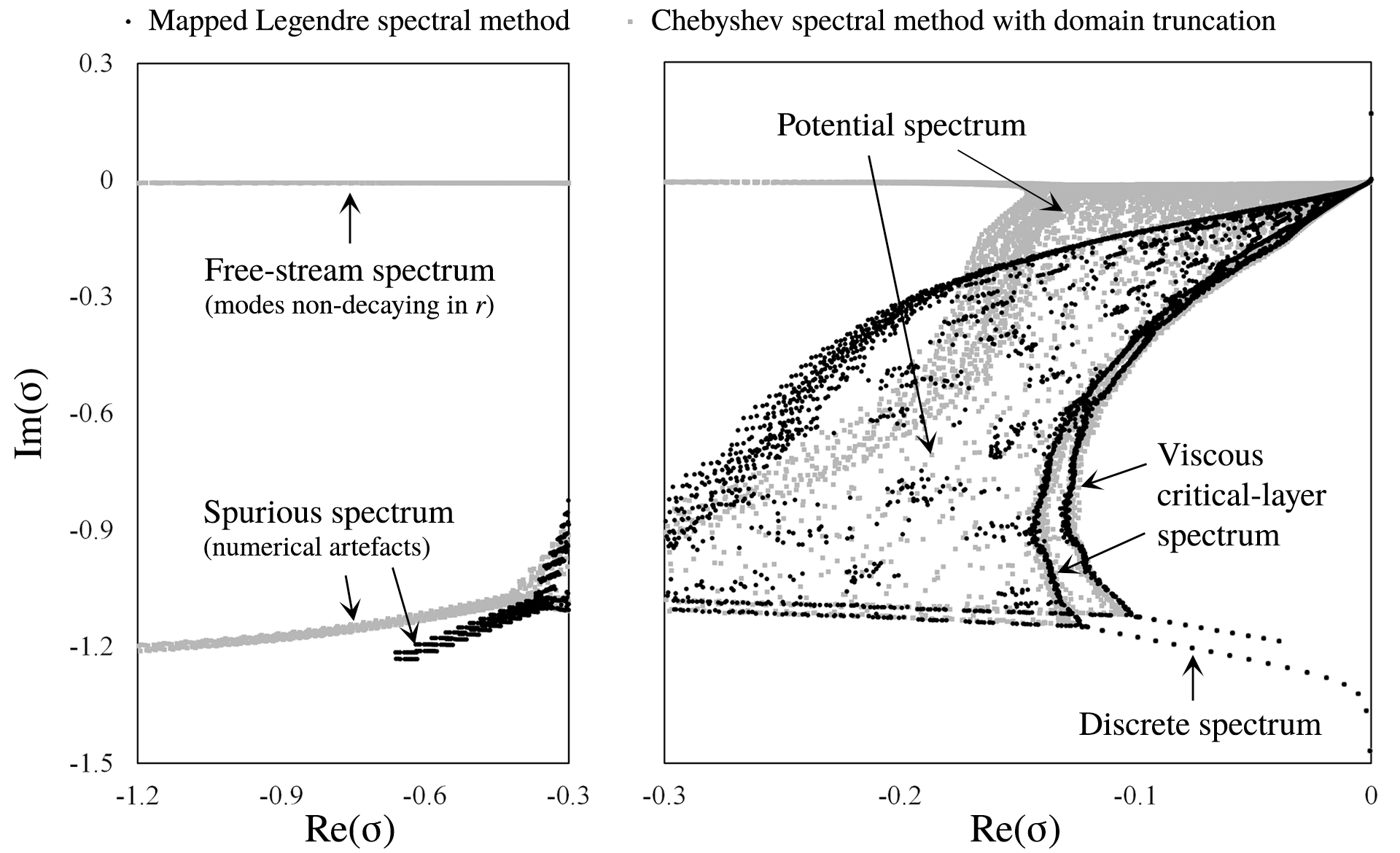
Figure 1: Numerical spectra of the $q$-vortex with $(m,\,\kappa,\,q,\,\Rey)=(1,\,1.0,\,4.0,\,10^{5})$ using the Chebyshev spectral collocation method (grey squares), and the mapped Legendre spectral collocation method (black dots). The consistency of the discrete spectrum attests the robustness of the two methods. The free-stream and spurious spectra (in the left panel) are associated with either singular or non-physical eigenmodes, thus superfluous for this study. Most of them are generated by the Chebyshev spectral method. The discrete, potential and viscous critical-layer spectra (in the right panel) are associated with regular eigenmodes. Two curves of the viscous critical-layer spectrum are more distinctive via the mapped Legendre spectral method.

A couple of issues arise when we choose the Chebyshev spectral method over the mapped Legendre spectral method to resolve the eigenmodes. First of all, as depicted in the left panel of figure 1, a significant portion of the numerically resolved spectra account for the eigenmode families either singular or non-physical, which are solely redundant for the present problem. This issue is most likely to stem from approximating the asymptotic constraints to the subordinate boundary conditions at both ends of the computational domain. In the Chebyshev spectral method, as for $m=1$, we have implemented the boundary conditions of

$$\frac{d\tilde{u}_{r}}{dr}=\frac{d\tilde{u}_{\phi}}{dr}=\tilde{u}_{z}=\tilde{p}=0~{}~{}~{}~{}\text{at}~{}~{}r=0,$$ (3.1)

and

$$\tilde{u}_{r}=\tilde{u}_{\phi}=\tilde{u}_{z}=\tilde{p}=0~{}~{}~{}~{}\text{at}~{}~{}r=R_{\infty},$$ (3.2)

which are proxies for the analyticity at the origin and the rapid decay condition as $r\rightarrow\infty$, respectively (see Ash & Khorrami, 1995). Even though (3.1) and (3.2) may serve as necessary conditions for what they are supposed to mimic, they can never be considered formally equivalent. For instance, (3.2) does not prohibit solutions from oscillating in the far field as long as the oscillation is momentarily zeroed out at $r=R_{\infty}$, which explains the emergence of the free-stream spectrum.

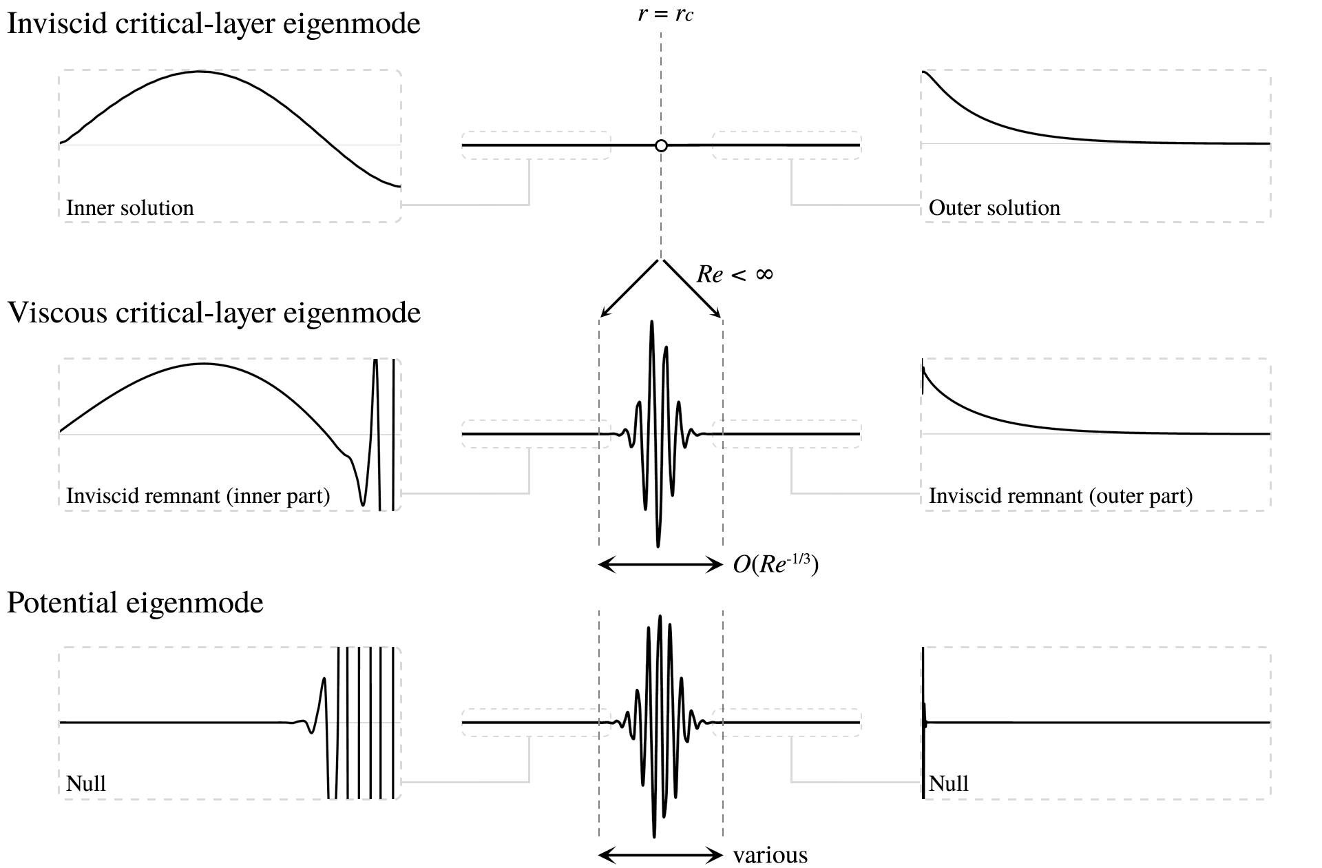
Figure 2: Schematic comparison between viscous critical-layer and potential eigenmodes. Both exhibit a similar large-scale structure in the region where the viscosity effect is locally dominant, which corresponds to a singularity at $r=r_{c}$ in the inviscid limit. The width of this large-scale structure scales as $O(Re^{-1/3})$ (see Lin, 1955) for the viscous critical-layer eigenmode. In contrast, for the potential eigenmode, the width can vary even at the same $Re$. The potential eigenmode forms a ‘wave packet’ in compliance with the pseudomode analysis (see Trefethen & Embree, 2005). Aside from the location $r=r_{c}$, the viscous critical-layer eigenmode inherits the structure of its inviscid counterpart, while the potential eigenmode just turns into null.

The second issue comes with the unclear distinction between the viscous critical-layer spectrum and the potential spectrum. As discussed in Lee & Marcus (2023, pp. 41-42), the Chebyshev spectral method produces scattered traces of the two curves of the viscous critical-layer spectrum, making it less clear to distinguish the curves from the surrounding continuous region. This scattering can be attributed to the high sensitivity of the continuous spectra even to minor errors. In the Chebyshev spectral method, the domain truncation removes any spatial information apart from the origin, which, albeit diminutive, holds physical significance. Figure 2 illustrates the difference between the viscous critical-layer eigenmodes and the potential ones. Despite their structural resemblance on a large scale, the viscous critical-layer eigenmodes maintain the structure of their inviscid counterparts outside the region where viscosity effect dominates locally, scaled in the order of $Re^{-1/3}$ (Lin, 1955). In contrast, the potential eigenmodes just turns into null outside this region, epitomising their ‘wave packet’ form (Mao & Sherwin, 2011) which conforms to the twist condition presented by Trefethen & Embree (2005, pp. 98-114). More details of their comparison are omitted here; they have been elucidated in Lee & Marcus (2023).

A numerical sensitivity test involving the evaluation of the maximum energy growth $G$ at $\tau=10$ from the entire eigenspace using the two methods is presented in figure 3. The other physical parameters remain the same: $(m,\,\kappa,\,q,\,\Rey)=(1,\,1.0,\,4.0,\,10^{5})$. Unsurprisingly, increasing the number of spectral elements $M$ enables both methods to be less sensitive to changes in numerical parameters. At a fixed $M$, the map parameter $L$ serves as a resolution tuning parameter in the mapped Legendre spectral collocation method, and the domain truncation radius $R_{\infty}$ in the Chebyshev spectral collocation method. Note that the test ranges shown in figure 3 are based on the typical usage for each parameter as found in Lee & Marcus (2023) and Mao & Sherwin (2011), respectively. Changes in $L$ by and large do not affect $G(\tau=10)$ in the test range of the mapped Legendre spectral collocation method ($1\leq L\leq 10$). Therefore, we may arbitrarily choose $L$ within this range. On the contrary, $G(\tau=10)$ is affected by changes in $R_{\infty}$ in the test range of the Chebyshev spectral collocation method ($10\leq R_{\infty}\leq 20$), particularly as $R_{\infty}$ increases. This is problematic because using a large $R_{\infty}$ should be preferred to minimise its detrimental influence on the unbounded nature of the radial domain. We observed that this problem is mitigated by manually excluding the sub-eigenspace spanned by the free-stream eigenmodes, which is, in fact, proactively removed in the mapped Legendre spectral collocation method. We believe that the exclusion is reasonable from a physical standpoint because the non-decaying behaviour of the free-stream eigenmodes implies that they analytically possess infinite energy. This, in turn, renders them formally inapplicable in the current transient growth context.

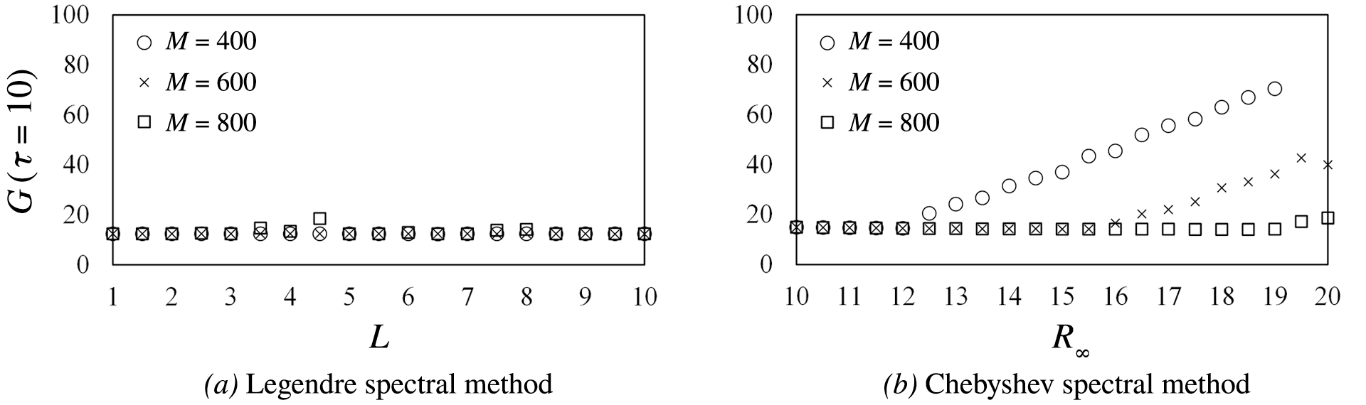
Figure 3: Numerical sensitivity test by evaluating $G(\tau=10)$ from the entire eigenspace associated with $(m,\,\kappa,\,q,\,\Rey)=(1,\,1.0,\,4.0,\,10^{5})$ using $(a)$ the mapped Legendre spectral collocation method with varying $L$, and $(b)$ the Chebyshev spectral collocation method with varying $R_{\infty}$, for $M=400,\,600$ and $800$. The test ranges are based on typical usage for each parameter. Setting a finite $R_{\infty}$ fundamentally damages the unbounded nature of the problem, and therefore, a large $R_{\infty}$ should be preferred, while $L$ can be arbitrarily chosen without impacting the unboundedness of the domain. However, as $R_{\infty}$ increases, the evaluation is undesirably numerically sensitive.

To recapitulate, when it comes to resolving the eigenmodes of the $q$-vortex in a radially unbounded domain, the Chebyshev spectral method has a couple of issues resulting from domain truncation, and they unfavourably affect the numerical sensitivity with respect to transient growth evaluation. Instead, the mapped Legendre spectral method can be an effective alternative to overcome these numerical limitations, making it more suitable for the current problem. Consequently, we choose the mapped Legendre spectral collocation method to analyse the transient growth of the wake vortex.

3.2 Maximum energy growth

Mao & Sherwin (2012) demonstrated that transient growth primarily results from the non-normality of the continuous eigenmodes, while the discrete eigenmodes play a less significant role. Here, they used the term ‘continuous eigenmodes’ as a compilation of the potential and free-stream families. However, as we pointed out earlier, the free-stream eigenmodes may not be appropriate for evaluating maximum energy growth because their energy reaches infinity. Therefore, in their argument, ‘continuous eigenmodes’ should be more specifically referred to as the potential ones. Not only that, but their argument also requires further refinement because they overlooked the viscous critical-layer eigenmodes. In their classification, this eigenmode family was not distinguished from the potential family, presumably due to the overlap in the spectra of these two families (see Mao & Sherwin, 2011, p. 8), as well as their structural similarity on a large scale (see figure 2).

Accordingly, the argument put forth by Mao & Sherwin (2012) still necessitates further clarification regarding which continuous eigenmode family primarily contributes to the optimal perturbation leading to maximum energy growth: the potential family or the viscous critical-layer family. To that end, we first evaluate the values of $G(\tau)$ from the entire eigenspace and then compare them with those from different sub-eigenspaces respectively spanned by a distinct eigenmode family.

Figure 4 shows the plots of numerically evaluated values of $G(\tau)$ from the entire eigenspace at various wavenumbers $\kappa$ for the $m=0$ and $m=1$ cases, respectively. In the cases of $m=0$, where the perturbations are essentially two-dimensional (i.e., subject only to $r$ and $z$), the dependence of the $G$ curves on $\kappa$ is clear and monotonous. In the short run, the growth is strong with large $\kappa$, whereas in the long run, the largest $G$ is obtained with smaller values of $\kappa$. One may check in figure 4$(a)$ that the upper envelope of all curves sequentially corresponds to the curves with decreasing $\kappa$ as $\tau$ increases. This trend at $m=0$ aligns with previous observations in the literature (Pradeep & Hussain, 2006; Mao & Sherwin, 2012), supporting the validity of our evaluation. When it comes to $m=1$, with three-dimensional perturbations, the $\kappa$-dependence of the $G$ curves is no longer monotonous, as previously reported in Antkowiak & Brancher (2004). Focusing on a relatively short-term growth, we can see that the largest $G$ at $m=1$ is generally greater than that at $m=0$. For example, at $\tau=10^{2}$, the largest $G$ among the evaluated values is $7.5\times 10^{2}$ for $\kappa=0.1$ at $m=1$, while it is $2.8\times 10^{2}$ for $\kappa=5.0$ at $m=0$.

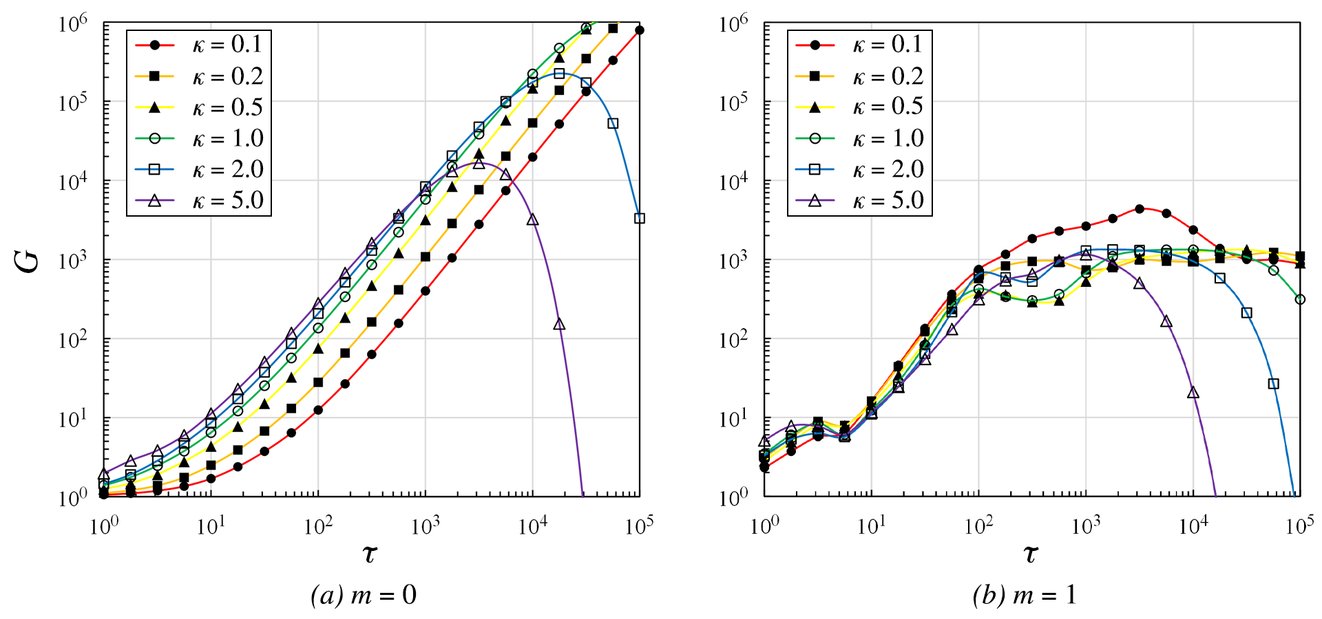
Figure 4: Maximum energy growth with respect to total growth time $(a)$ at $m=0$ (axisymmetric) and $(b)$ at $m=1$ (helical). The values of $G$ are evaluated from the entire eigenspace, whose basis elements involve the whole discrete, potential and viscous critical-layer families. Here, $q=4$ and $\Rey=10^{5}$.

The maximum energy growth curves evaluated from the entire eigenspace and the sub-eigenspaces, each respectively spanned by the discrete family, the viscous critical-layer family and the potential family, are compared in figure 5. It is clear that the curves from the entire eigenspace are mainly reproduced by those evaluated from the sub-eigenspace spanned by the viscous critical-layer family, indicating its dominant contribution. On the other hand, the values of $G(\tau)$ from the rest of the continuous sub-eigenspace, for which the potential eigenmodes account, exhibit a similar order of magnitude to those from the discrete sub-eigenspace. The contribution of the potential family is, therefore, as minor as that of the discrete family in transient growth.

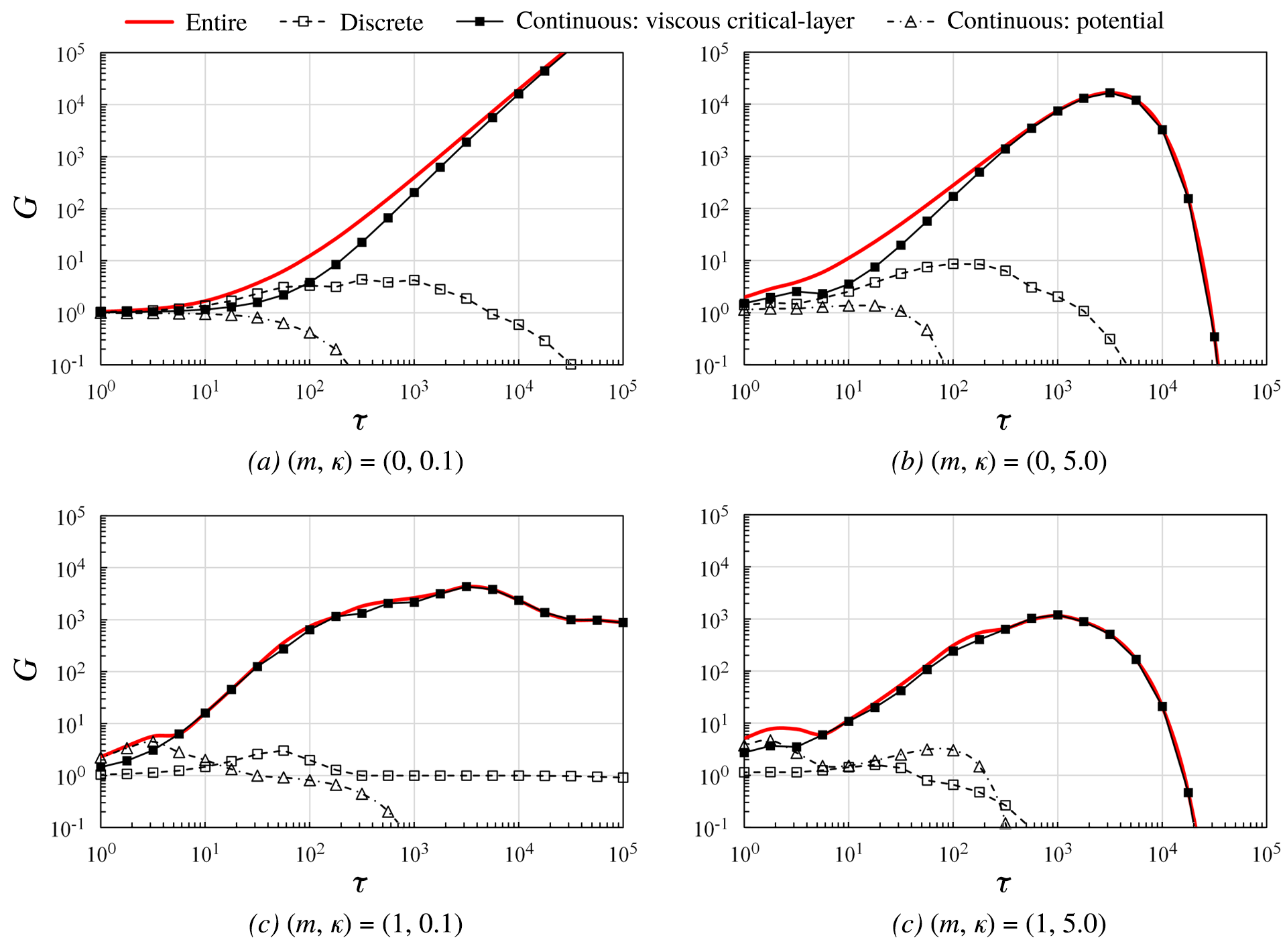
Figure 5: Comparison of the curves of $G(\tau)$ evaluated from different sub-eigenspaces, each respectively spanned by a distinct eigenmode family: $(a)$ $(m,\,\kappa)=(0,\,0.1)$, $(b)$ $(m,\,\kappa)=(0,\,5.0)$, $(c)$ $(m,\,\kappa)=(1,\,0.1)$, and $(d)$ $(m,\,\kappa)=(1,\,5.0)$. Here, $q=4$ and $\Rey=10^{5}$. The maximum energy growth curves from the entire eigenspace are the same as those plotted in figure 4, which are mainly reproduced by those evaluated from the sub-eigenspace spanned by the viscous critical-layer family.

There are two minor exceptions worth noting. At $m=0$, the discrete family accounts for short-term optimal growth as significantly as the viscous critical-layer family, especially when $\kappa$ is small. We believe that this is relevant to the fact that when $m=0$, critical layers vanish in the limit of $\kappa\rightarrow 0$, and so do the derived continuous eigenmodes, while the discrete ones remain. Next, at $m=1$, the contribution of the potential family to optimal growth slightly supersedes that of the viscous critical-layer family for a brief period ($\tau<10$), explaining the presence of a quirk in the $G$ curves around $\tau=5.6$. However, the exception clears quickly after this period, and the largest $G$ attainable in this period never exceeds $10$, thus not overturning the general dominance of the viscous critical-layer family in terms of transient growth.

Based on these observations, we revisit the demonstration provided by Mao & Sherwin (2012) with the following clarification; the non-normality of the continuous eigenmodes induces significant transient growth, and more precisely, it is the viscous critical-layer family that predominantly contributes to this growth, instead of the potential family. The distinction is important as it addresses the ‘true’ origin of transient growth of the wake vortex as critical layers. The potential eigenmodes have their theoretical foundation in the wave packet pseudomode analysis (Trefethen & Embree, 2005). As showcased in figure 2, they omit the asymptotic information of critical layers, making their birth irrelevant to those requiring asymptotic matching or equivalently, the critical layer analysis (Lin, 1955; Le Dizès, 2004). Although the wave packet pseudomode analysis is deemed to be a powerful tool to explore all possible forms of continually varying eigensolutions, it may divert our attention too much from the genuine gems more worthy of our focus. Furthermore, our clarification provides a better alignment with the previous argument made by Heaton (2007b) that inviscid continuous spectrum (CS) transients dominate the growth over short time intervals. The viscous critical-layer family in our classfication corresponds to the viscous regularisation of the inviscid CS, which we have denoted the inviscid critical-layer spectrum (Lee & Marcus, 2023), when $\Rey<\infty$.

3.3 Perturbation structures

The impact of changes in $m$ and $\kappa$ on perturbation structures leading to optimal transient growth has been widely investigated and is well-known in the context of linear vortex dynamics (Antkowiak & Brancher, 2004; Pradeep & Hussain, 2006; Mao & Sherwin, 2012). In this section, we examine whether our transient growth calculation complies with the established findings and then compare and analyse the perturbation structures with respect to different values of $m$ and $\kappa$ for further consideration.

Pradeep & Hussain (2006) reported that axisymmetric perturbation cases ($m=0$) generally exhibit the largest energy growth, as we showed in figure 4. However, as the largest $G$ increases, the total growth period of the perturbation is monotonously extended (i.e., $\tau$ required to achieve $G$ increases), as its spatial structure becomes increasingly distant from the vortex core, resulting in slower interactions. For helical perturbation cases ($m=1$), a common spatial structure emerges, with the primary motion localised around a certain radius near the vortex core. In the case of $m=1$ perturbations, it is noteworthy that their growth may lead to the initiation of vortex core fluctuations, even though they initially originate outside the core. This mechanism has occasionally been considered a trigger of erratic long-wavelength displacements in experimental vortices (e.g., Edstrand et al., 2016; Bölle et al., 2023), referred to as ‘vortex meandering’ (see Antkowiak & Brancher, 2004, p. L4). Mao & Sherwin (2012) found that the vortex meandering phenomenon can be driven by the transient response of the vortex to an out-of-core perturbation.

As mentioned in §2.3, our focus is on the relatively short time period of $10<\tau\leq 100$ to study the transient growth process. In longer periods, classical linear instability mechanisms like the Crow instability may predominate in real conditions. Within this time range, the largest values of $G$ attained from our considerations (see figure 4) occur at $\kappa=5.0$ for the $m=0$ cases and at $\kappa=0.1$ for the $m=1$ cases. We consider these cases as representative. In figure 6, we illustrate the optimal perturbation velocity inputs and outputs for $\tau=31.6$ and $\tau=100$, all of which are depicted by the absolute velocity components. For more intuitive visualisation, we portray their corresponding three-dimensional structures alongside, each of which is represented by the iso-surface of 50% of the maximum specific energy in physical space, i.e., $|(\tilde{\bm{u}}(r)e^{\mathrm{i}(m\phi+\kappa z)}+\mathrm{c.c.})/2|^{2}$, where $\mathrm{c.c.}$ stands for the complex conjugate of the antecedent term. The dark and light surface colours respectively express counterclockwise and clockwise swirling directions.

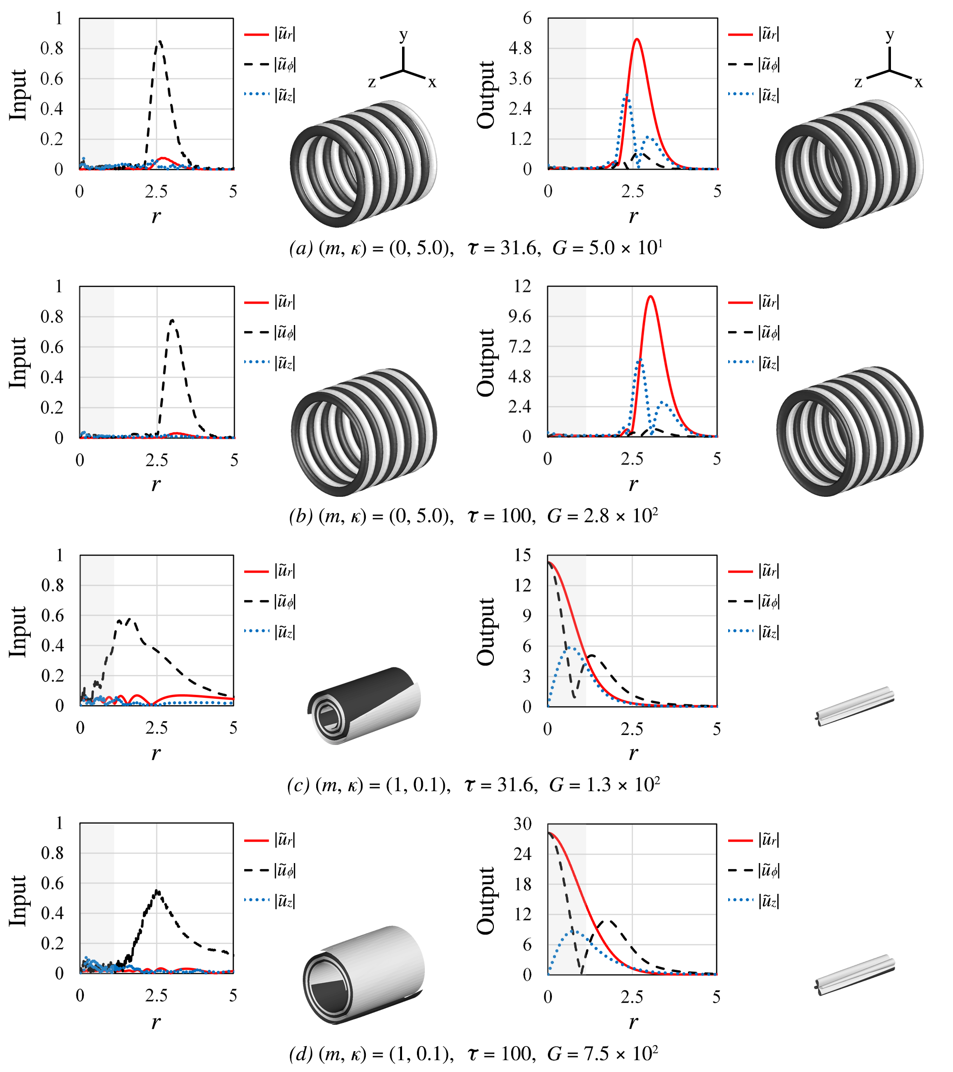
Figure 6: Optimal perturbation inputs of unit energy $E$ defined in (2.7) and amplified outputs at $t=\tau$, depicted by the absolute velocity components alongside their corresponding three-dimensional structures, each represented by the isosurface of 50% of the maximum specific energy in space. The dark and light colours respectively indicate counterclockwise and clockwise swirling of the flow at each position. Here, four representative cases with the largest value of $G$ in figure 4 are displayed: $(a,\,b)$ the axisymmetric cases of $(m,\,\kappa)=(0,\,5.0)$ for $\tau=31.6$ and $\tau=100$, respectively, and $(c,\,d)$ the helical cases of $(m,\,\kappa)=(1,\,1.0)$ for $\tau=31.6$ and $\tau=100$, respectively. The initial dominance of azimuthal velocity components is common to all cases, and that for $m=1$, energy is transferred into the core region $r\leq 1.12$ (shaded in each plot).

In all cases, the following characteristics are commonly observed. First, azimuthal velocity components are initially dominant for all optimal perturbations, while the other velocity components evolve significantly towards the end of the growth period. This clearly indicates that the azimuthal velocity component should be the primary focus if one intends to induce these optimal perturbations from the unperturbed state. Second, the most energetic part of the optimal perturbation inputs, coinciding with the peak of the absolute azimuthal velocity component, tends to be distant from the vortex core as $\tau$ increases. One may see a considerable difference particularly for cases $(c)$ and $(d)$, as the major perturbation structure overlaps the core region when $\tau=31.6$ whereas it moves out of the core when $\tau=100$.

For cases $(a)$ and $(b)$, where $(m,\,\kappa)=(0,\,5.0)$, the input perturbations generally form a ring structure owing to its azimuthal independence. As the perturbation develops, it is evident that the radius of the ring does not change significantly. Taking into account other cases with different wavenumbers (even besides the illustrated ones), we found this tendency toward local confinement of optimal perturbation structures to take place in general with increasing $\kappa$. This indicates that a perturbation with a shorter axial wavelength has a more localised influence around the initially perturbed region.

For cases $(c)$ and $(d)$, where $(m,\,\kappa)=(1,\,0.1)$, a spiral structure emerges in the most energetic region of the input perturbation due to the alternating layering of two oppositely swirling fluid motions at the periphery of the vortex core. Unlike the axisymmetric cases, the perturbation structure undergoes a drastic change when comparing its input and output states. Specifically, the most energetic region of the perturbation, even if it was originally located outside the vortex core, ultimately penetrates into the vortex core. As a consequence, the transverse velocity ($\tilde{u}_{r}$ and $\tilde{u}_{\phi}$) at the vortex centre becomes the greatest. In other words, the principal response of the vortex to optimal perturbations with $m=1$ is transverse motion of the vortex core, which is likely to be connected with the vortex meandering phenomenon (Edstrand et al., 2016; Bölle, 2021).

We want to clarify that the finding regarding the induction of vortex meandering by optimal helical perturbations with an axially long wavelength was formerly given by Mao & Sherwin (2012). They employed mesh-based direct numerical simulations instead of the matrix-based analysis (corresponding to (2.6) - (2.15) in our formulation), even though they used the matrix-based approach when $m=0$. In a way, this choice seems to have been made to overcome difficulties in dealing with analyticity at the origin, which depends on the value of $m$ (see Lee & Marcus, 2023, pp. 51-52). On the other hand, our approach, based on the mapped Legendre spectral collocation method, is fundamentally designed to remain robust for any value of $m$. Therefore, our contribution here lies in recognising the same phenomenon linked with $m=1$ perturbations based on the computationally fast and formally consistent matrix-based transient growth analysis.

3.4 Non-linear impacts on an optimally perturbed vortex

Given an optimally perturbed vortex, the linearised theory (see §2.1) predicts that the perturbation is gradually amplified as time approaches $t=\tau$ and then decays as far as there are no extrinsic factors to give rise to secondary instabilities starting from the most perturbed state. We spare this section for verifying that such transient behaviour still takes importance in the original non-linear system, complying with (2.2), in spite of energy transfer across different wavenumbers or relevant non-linear effects.

Although the optimal perturbation structures vary with the selection of $m$, $\kappa$ and $\tau$, what we aim to investigate here is their comprehensive and common trend of evolution in time anticipated in the linearised theory. We pay attention to one specific optimal perturbation case where $(m,\,\kappa)=(1,\,0.1)$ with the optimal growth time $\tau=50$, where the $z$-component of the perturbation vorticity input $\omega^{\prime}_{z}(t=0)$ on the $z=0$ plane is illustrated in figure 7. This perturbation is chosen because the drastic transition of the most energetic portion of the perturbation from the periphery to the vortex core, as shown in figure 6$(c,\,d)$, may be a good means to a plain illustration of the vortex growth. We emphasise that, however, this specific behaviour at $m=1$ (presumably related to vortex meandering) itself is not the target of interest at this point. To those who are interested in the meandering of vortices, we suggest referring to Edstrand et al. (2016) and Bölle (2021).

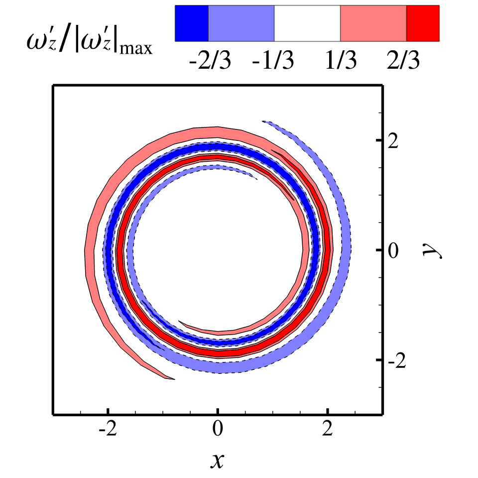
Figure 7: Axial perturbation vorticity contour on the $z=0$ plane of the optimal input where $(m,\,\kappa)=(1,\,0.1)$ with the optimal growth time $\tau=50$. The contour lines are solid for the positive levels (-67 % and -33 % of the absolute maximum) and dashed for the negative levels (33 % and 67 % of the absolute maximum).

According to the linearised theory, the optimal perturbation velocity input, which can be expressed as $\tilde{\bm{\upsilon}}_{\text{opt}}(0)=\mathsfbi{P}\mathsfbi{V}\mathsfbi{F}^{-1}\bm{r}_{1}$ as in (2.15), evolves at $t=\eta$ as

$$\tilde{\bm{\upsilon}}_{\text{opt}}(\eta)=\mathsfbi{P}\mathsfbi{V}\exp(\eta\mathsfbi{S})\mathsfbi{F}^{-1}\bm{r}_{1}.$$ (3.3)

One may check the consistency of the above equation when $\eta=\tau$ with $\tilde{\bm{\upsilon}}_{\text{opt}}(\tau)$ given in (2.15). We label this prediction from the linearised theory as ‘linear.’ The ‘linear’ prediction, however, may be ideal as it strips off all higher-order interactions coming from the non-linear convection term, i.e., $\bm{u}\times\bm{\omega}$ in (2.2), which transfers energy from the perturbation wavenumbers of $(m,\,\kappa)$ to the multiples (e.g., $(2m,\,2\kappa)$, $(3m,\,3\kappa),\,\cdots$) or vice versa. We refer to the growth of the optimal perturbation in consideration of the influence of higher-order interactions as ‘non-linear.’ The significance of this non-linearity substantially depends on the initial perturbation’s energy level. If the perturbation energy approaches zero (or the perturbation is infinitesimal), the ‘non-linear’ evolution should follow the ‘linear’ prediction. We set aside the numerical details regarding our non-linear simulations in Appendix B.

In the non-linear simulations, the initial velocity field $\bm{u}(t=0)$ is defined as follows:

$$\bm{u}(r,\phi,z,t=0\,;\,\varepsilon)\equiv\overline{\bm{U}}(r)+\varepsilon\tilde{\bm{u}}_{\mathrm{opt}}(r)e^{i(m\phi+\kappa z)}+\mathrm{c.c.},$$ (3.4)

where $\varepsilon$ determines how intense the initial perturbation is, adjusting the perturbation energy input. The base term representing the unperturbed $q$-vortex, $\overline{U}(r)$, has been assumed to be unchanging in time in the linear analysis, as its radial diffusion due to viscosity is negligible due to the high $Re$ number in our problem setup. In contrast, the non-linear simulations take this small viscous diffusion effect of the base $q$-vortex into account for accuracy purposes. That is to say, even the unperturbed flow changes slowly with respect to time. This can be calculated as the non-linear simulation with $\varepsilon=0$. As a result, the perturbation velocity field at $t=\eta$ is assessed as the difference between two time-varying fields, i.e.,

$$\bm{u}^{\prime}(r,\phi,z,\eta\,;\,\varepsilon)\equiv\bm{u}(r,\phi,z,\eta\,;\,\varepsilon)-\bm{u}(r,\eta\,;\,0).$$ (3.5)

The perturbation energy at $t=\eta$, denoted $E(\eta)$, is evaluated as the volume integration of $\bm{u}^{\prime}\cdot\bm{u}^{\prime}$ divided by $2\pi$ times the axial wavelength ($=2\pi/\kappa$), for the consistency with our energy definition in (2.7).

In figure 8, three energy growth curves are plotted together for comparison. First, the energy growth curve in the linear evolution case peaks at $t=\tau=50$. In this case, the maximum energy growth $G$ is $2.5\times 10^{2}$. This curve serves as an index of the prevalence of the linear process during early transient growth of vortices. Second, the energy growth curve in the non-linear evolution case with $E(0)=10^{-8}$ is almost identical to the ‘linear’ index curve. In this case, the non-linearity should be considered but only in an infinitesimal manner and its influence appears to be marginal. The only notable exception is a debilitation of the maximum energy growth at $t=\tau=50$. However, it is unlikely that this debilitation is entirely due to the introduction of non-linearity because, according to Mao & Sherwin (2012, p. 55), such a drop in energy growth at the peak appears to stem from the consideration of viscous diffusion of the base flow in time. Lastly, the energy growth curve in the non-linear evolution case with $E(0)=10^{-3}$ exhibits more debilitation at the peak even than the prior non-linear case. Unlike the previous case, this demonstrates the clear intensification of the non-linearity. Nevertheless, the overall trend of the curve does not drift away from that of the ‘linear’ index curve. The coherence in trend holds particularly well until the maximum vortex growth ($t<\tau=50$), which means that the linearised theory on transient growth is still effective in the original non-linear system.

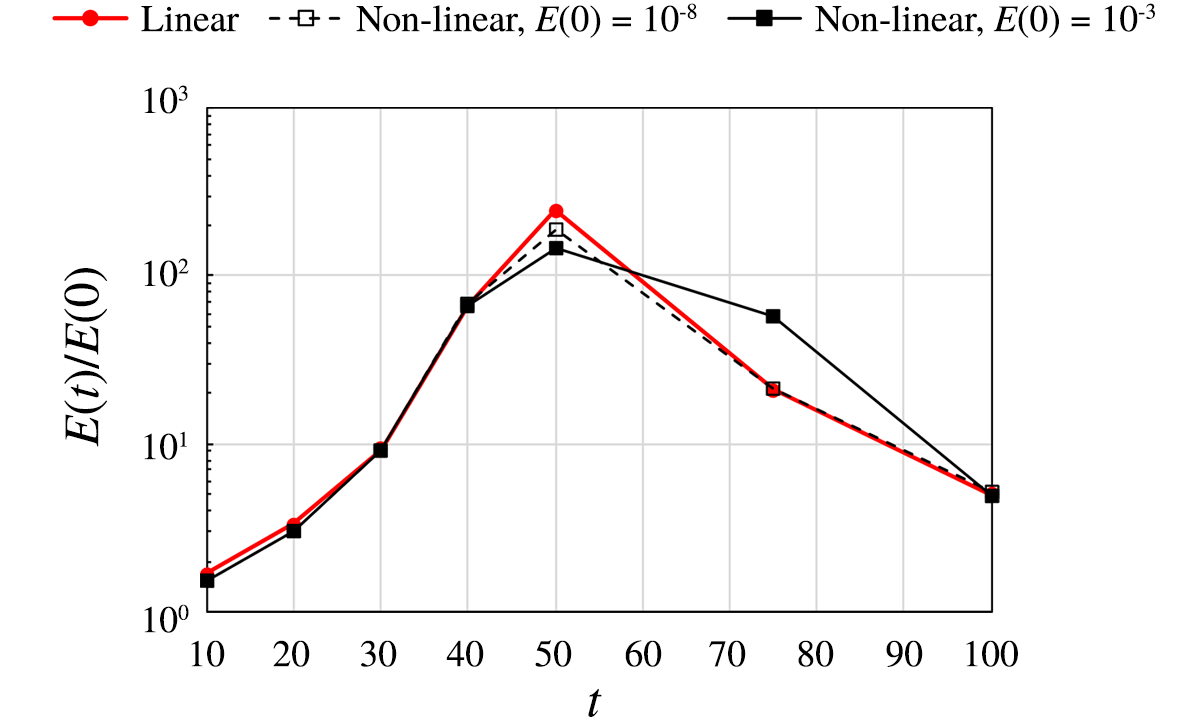
Figure 8: Comparison of the transient energy growth curves in the ‘linear’ evolution case, calculated via (3.3), and in the ‘non-linear’ evolution cases with the initial perturbation energy of $10^{-8}$ and of $10^{-3}$, calculated via three-dimensional non-linear simulations. The initial perturbation is illustrated in figure 7.

The prevalence of the linear process in the early-stage vortex growth is much clear when we take a look at the evolution of the perturbation structure, which is shown in figure 9. Using the same contour style across the three different cases presented above, we illustrate three snapshots of the axial vorticity perturbation contours on the $z=0$ plane at $t=25$, $t=50$ and $t=100$ for each case. The structural coherence in vorticity perturbation between the linear and non-linear cases is evident at $t=25$, representing the stage of rapid perturbation growth. At $t=50$, or the optimal growth time, the perturbation structures are still comprehensively coherent. However, in the non-linear evolution case with $E(0)=10^{-3}$, it can be found that the $m=1$ symmetry weakly breaks up, which means that the other azimuthal wavenumbers rather than $m=1$ begin to possess non-negligible energy via the higher-order energy transfer across different wavenumbers. At $t=100$, representing the stage of asymptotic stabilisation, the perturbation structures no longer show strong resemblance. This is another evidence of the non-linearity intensification particularly as a result of prolonged vortex growth in time.

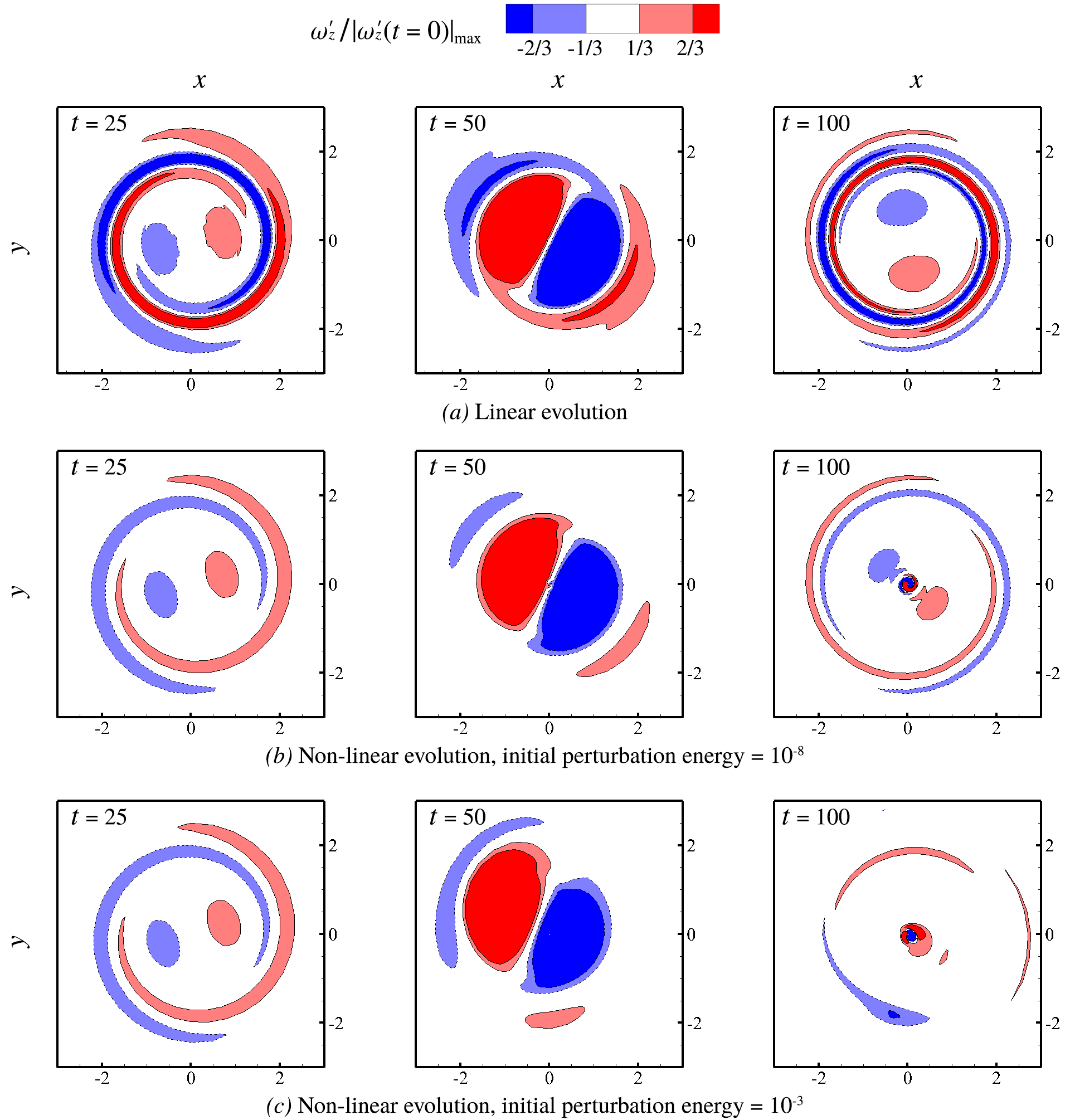
Figure 9: Axial vorticity perturbation contours of the optimally perturbed vortex (refer to figure 7 for the illustration of the initial perturbation) on the $z=0$ plane at $t=25$, $t=50$ and $t=100$: $(a)$ the ‘linear’ evolution case where the maximum energy growth is known to occur at $t=\tau=50$, $(b)$ the ‘non-linear’ evolution case with the initial perturbation energy of $10^{-8}$, $(c)$ the ‘non-linear’ evolution case with the initial perturbation energy of $10^{-3}$. The same contour style as figure 7 is applied to all plots. Despite the non-linearity and its intensification with an increase in perturbation energy or in time, the ‘linear’ process still prevails the overall dynamics with respect to early vortex growth in the original non-linear system.

Last but not least, we note that the simulation with the initial perturbation energy of $10^{-3}$ results in the substantial displacement of the vortex core, as shown in figure 10, notwithstanding the seemingly small level of energy. The $\lambda_{2}$-isosurface where $\lambda_{2}=-0.05$ is used to detect the vortex core (see Jeong & Hussain, 1995). The largest displacement of the vortex centre in the simulation is nearly equal to the core radius, coinciding with the experimentally observed meandering amplitude in the order of the core radius (see Devenport et al., 1997; Bölle, 2021). Based on the rough figures of a large transport aircraft given in Fabre & Jacquin (2004, p. 259), the characteristic scales in our formulation become $U_{0}\approx 27~{}\mathrm{m/s}$ and $R_{0}\approx 0.5~{}\mathrm{m}$ and using the density of air $\rho\approx 1~{}\mathrm{kg/m^{3}}$, the ‘dimensionless’ energy of $10^{-3}$ corresponds to the ‘actual’ kinetic energy of $(10^{-3})\times 2\pi\rho(U_{0}^{2}/2)R_{0}^{2}\approx 0.6~{}\mathrm{J/m}$ (‘per metre’ stands for the axial unit length), which appears to be not exorbitant in practice. We believe this strengthens the practicability of the optimal transient growth process under consideration, arguably owing to the radially concentrated nature of the optimal perturbation structures (see figure 7).

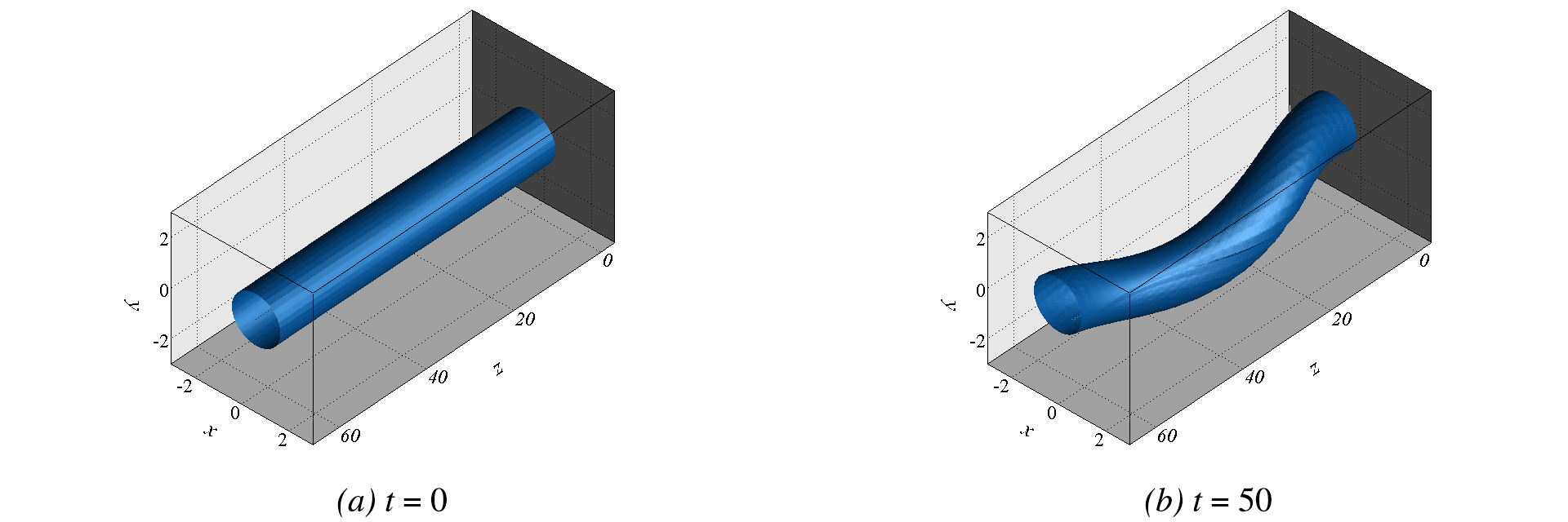
Figure 10: Three-dimensional illustration of the $q$-vortex with the helical perturbation (see figure 7) of the initial energy of $10^{-3}$: $(a)$ the initial core ($t=0$), and $(b)$ the most excited core ($t=\tau=50$). To detect the vortex core, the $\lambda_{2}$-isosurface where $\lambda_{2}=-0.05$ is depicted (see Jeong & Hussain, 1995). The maximum displacement of the vortex centre comes up to the order of the core radius, which is as substantial as the experimental meandering amplitude (see Devenport et al., 1997; Bölle, 2021).

4 Initiation of optimal transient growth

4.1 On a means of initiating optimal transient growth

The transient evolution of the optimally perturbed $q$-vortex that we have analysed in the previous section unveils a promising way to significantly disturb the vortex even if the base vortex is known to be linearly stable. For this growth process to be practically meaningful, an important question remains: By what means is the perturbation initiated? In our analyses and simulations thus far, perturbations have been presumed to be initially present along with the vortex, which is supposed to be initially in an undisturbed state. However, from a practical standpoint, there should be a means of causing such perturbations because they cannot originate from the undisturbed flow — the $q$-vortex, which by itself is quasi-steady. Without a plausible initiation process, the optimal transient vortex growth process may be no more than hypothetical.

One may consider ambient turbulence as a compelling explanation for initiation, as often addressed in the linear instability context (e.g., Crow & Bate, 1976; Han et al., 2000). However, in contrast to linear instability mechanisms, where we anticipate that perturbations are destined to be explosive in the limit of $t\rightarrow\infty$ due to the most unstable eigenmode growing in an exponential manner, a transient growth process typically necessitates a specific (optimal) form of perturbation as input. The issue of whether such a specific perturbation can spontaneously originate from ambient turbulence, which is fundamentally stochastic and uncontrolled, has led to recurrent criticisms of optimal transient growth (see Fontane et al., 2008, p. 235). In the work by Fontane et al. (2008), where the transient dynamics of vortices with stochastic forcing was analysed, they confirmed the activation of optimal perturbations by noise-like forcing that is random in both space and time. This mitigates the aforementioned criticisms of optimal transient growth. Nonetheless, as the authors stated, it remains questionable whether such random isotropic forcing effectively represents turbulence in real conditions. The lack of clear universality in modeling turbulence is believed to be an intractable challenge when incorporating ambient turbulence in the current problem.

Instead, we take the initiative in considering a different means of initiating optimal transient growth: ice crystals (or particles). Their presence in real life is ascertained through the observation of contrails. The formation of contrails primarily begins with jet exhaust plumes produced by aircraft engines, which contain particulate matter that sooner or later serves as condensation nuclei (Kärcher, 2018). We clarify that our focus does not lie in this very initial stage of contrails in the form of jet plumes. During this stage, the vortex roll-up process is underway, and, according to the early experimental study by El-Ramly & Rainbird (1977), there is no appreciable influence of the engine exhaust on the alteration of the rolled-up structure. As a matter of course, our attention is directed towards the later stage associated with a formed wake vortex, where the interaction between a vortex and ice crystals is manifest.

During the stage of ice crystals interacting with a wake vortex, the size of an individual particle reportedly comes up to a few microns (Kärcher et al., 1996; Paoli & Garnier, 2005; Naiman et al., 2011; Voigt et al., 2011; Kärcher, 2018). Due to its relatively small length scale compared to the vortex scale (in metres), the entire ice crystals are often treated as flow tracers, i.e., particles with no backward influence on the carrier fluid (Paoli & Garnier, 2005; Naiman et al., 2011). The assumption appears to be acceptable and efficiently simplifies the dynamics of the flow with particles. However, when considering the large particle number density, reportedly between $10^{9}$ per cubic metre to $10^{11}$ per cubic metre (Paoli et al., 2004; Paoli & Garnier, 2005), and the density ratio of ice to air (approximately $10^{3}$), the bulk effect of the ice crystals cannot be simply negligible. Under optimistic estimation based on the given figures, the upper limit of the particle mass fraction may fall in the range between $10^{-2}$ and $10^{-1}$. This amount is appreciable enough to initiate a perturbation that ultimately evolves into a substantial vortex disturbance via the transient growth process (recall §3.4).

When considering ice crystals in the development of contrails, the primary emphasis has typically centred on their microphysical growth. Consequently, the analysis often takes account of an ice microphysics model alongside a flow solver (e.g., Lewellen & Lewellen, 2001; Paoli et al., 2004; Paoli & Garnier, 2005; Naiman et al., 2011). However, this aspect is excluded from our consideration. Instead, we direct our attention to two-way coupling, specifically through drag momentum exchange. This approach aligns with our essential focus on examining the significance of the particles’ backward disturbance to the wake vortex. Recalling that azimuthal perturbations commonly dominate during initial optimal transient growth (see the left panels in figure 6), we speculate that momentum exchange via drag provides an effective means of initiating optimal perturbations, complementing ambient turbulence whose action is stochastic and, in an ideal sense, non-directional.

We note that, according to recent studies by Shuai & Kasbaoui (2022) and Shuai et al. (2022), weakly inertial particles within a vortex under two-way coupled conditions are found to be influential enough to trigger instabilities and expedite the vortex decay process. Although the initial particle distributions considered in these studies, where particles are loaded either over the entire domain or inside the vortex core region, are not directly applicable to our case, where particles interact with the vortex along the periphery of the vortex core, the studies support the underlying idea that even a dilute amount of particles meaningfully affects the surrounding vortex.

4.2 Two-way coupled equations for a vortex interacting with particles

To simulate the initiation process leading to the transient growth of a vortex via particle drag, we need to consider additional parameters and variables in order to establish an equation for the motion of particles. Also, we should add a coupling term to the momentum equation of fluid motion in (2.2) to complete a two-way coupled formulation. In our discussion, the particles under consideration are dispersed ice crystals, with a density roughly $10^{3}$ times greater than that of the surrounding fluid (air). We define the ratio of particle density $\rho_{p}$ to fluid density $\rho$ as a new dimensionless parameter, denoted by $\vartheta$ ($\equiv\rho_{p}/\rho$). We typically set $\vartheta$ to the constant value of $10^{3}$ in later calculations.

In this study, we employ the Eulerian approach adopting the fast equilibrium approximation, proposed by Ferry & Balachandar (2001). In this method, the set of particles is treated as continuum, allowing the flow-particle system to behave like a two-phase flow. Due to the high particle number density, we refrain from the use of Lagrangian approaches tracking particles individually (e.g., Paoli et al., 2004; Naiman et al., 2011; Shuai et al., 2022). Thanks to the relatively moderate computational cost, we believe the Eulerian approach is favourable for scale-up simulations, such as two or more vortices, to account for secondary vortex evolution in our future studies. Also, our focus on the ‘bulk’ influence of particles on the surrounding vortex, rather than individual particle statistics, fairly justifies the treatment of particles as continuum.

The following two variables now represent the particles in the form of dispersed phase: particle velocity field $\bm{u}_{p}(r,\phi,z,t)$ and particle volume fraction $c(r,\phi,z,t)$. The fast equilibrium approximation allows $\bm{u}_{p}$ to be explicitly evaluated in terms of the fluid velocity field $\bm{u}$. Based on the Maxey-Riley equation with the added mass effect (Maxey & Riley, 1983; Auton et al., 1988), $\bm{u}_{p}$ can be reduced in the resulting two-way coupled equations (see Ferry & Balachandar, 2001, p. 1221). They are

$$\frac{\partial\bm{u}}{\partial t}=-\bm{\nabla}\varphi+\bm{u}\times\bm{\omega}+\frac{1}{\Rey}{\nabla}^{2}\bm{u}-(\vartheta-1)c\frac{D\bm{u}}{Dt}~{}~{}~{}\text{with}~{}\bm{\nabla}\cdot\bm{u}=0,$$ (4.1)

and

$$\frac{\partial c}{\partial t}=-\bm{u}\cdot\nabla c+\frac{2{Stk}(\vartheta-1)}{2\vartheta+1}\nabla\cdot\left(c\frac{D\bm{u}}{Dt}\right),$$ (4.2)

where $D/Dt$ is the material derivative with respect to the fluid phase and $Stk$ is the Stokes number, i.e., the dimensionless particle relaxation time normalised by $R_{0}/U_{0}$. In calculations, we set $Stk=10^{-5}$ to comply with the fast equilibrium approximation as well as practical conditions (Kärcher et al., 1996). The discretisation and time-integration procedures for (4.1) and (4.2) are not different from the previous pure vortex cases, as detailed in Appendix B. Compared to (2.2), it can be seen that the last term in (4.1) represents the particle drag, whose magnitude depends upon the order of $c$.

4.3 Initial particle distribution

As briefly discussed above with the recent studies on vortex-particle interactions (Shuai & Kasbaoui, 2022; Shuai et al., 2022), the observable scope of vortex-particle interactions varies based on the initial distribution of particles. Accordingly, in order to substantiate that particle drag initiates optimal transient growth in the vortex, it is necessary to set up an effective initial distribution of the particles. We first remark that the role of particles here should be limited to small disturbance to the vortex system, which implies $(\vartheta-1)c$ significantly less than order unity in the following discussions.

To begin with, let’s comprehend how the particles induce perturbations in the carrier fluid. Reorganising the coupled momentum equation in (4.1), we obtain

$$\left(1+(\vartheta-1)c\right)\frac{D\bm{u}}{Dt}=-\bm{\nabla}p+\frac{1}{\Rey}{\nabla}^{2}\bm{u},$$ (4.3)

which is in fact the original form Ferry & Balachandar (2001) provided. In this form, it is clearly demonstrated that the combined motion of the two phases behaves like a single-phase flow with a slight density variation with a multiplication factor of $(1+(\vartheta-1)c)$. This effect is understood as a consequence of the dispersed phase absorbing momentum from the fluid phase. Loosely speaking, if the fluid accelerates, the presence of the particles retards the fluid’s acceleration and therefore results in negative perturbation velocity, and vice versa.

Given that the perturbation velocity is induced by non-zero $c$, we can derive from the velocity decomposition of (4.3) that

$$(\vartheta-1)c\frac{D\overline{\bm{u}}}{Dt}+\frac{D\bm{u}^{\prime}}{Dt}=-\bm{\nabla}p^{\prime}+\frac{1}{\Rey}{\nabla}^{2}\bm{u}^{\prime}.$$ (4.4)

It can be confirmed that (4.4) becomes identical to the total equation in (4.3) if $c=0$. Recalling that the aim is to investigate the initial particle distribution $c(t=0)$, denoted $c_{0}$, that effectively perturbs the ‘undisturbed’ vortex towards optimal transient growth, we assume zero perturbations at $t=0$. This makes (4.4) reduce to

$$\frac{\partial\bm{u}^{\prime}}{\partial t}\big{\rvert}_{t=0}=-(\vartheta-1)c_{0}\frac{D\overline{\bm{u}}}{Dt}\big{\rvert}_{t=0}.$$ (4.5)

Suppose that we aim to initiate a specific velocity perturbation $\breve{\bm{u}}^{\prime}$. If we find $c_{0}$ such that right-hand side of (4.5) coincides with (a positive constant multiple of) $\breve{\bm{u}}^{\prime}$, then we may expect $\bm{u}^{\prime}$ after a brief advancement in time to exhibit the perturbation in the form of $\breve{\bm{u}}^{\prime}$. The existence of such $c_{0}$ is rare since (4.5) in fact comprises three component equations whereas $c_{0}$ is the only unknown. We inevitably concentrate on the most important one among those in order to circumvent this overdetermination issue. If we choose the azimuthal component, the problem is converted into finding $c_{0}$ such that

$$-(\vartheta-1)c_{0}{\bigg{(}\frac{D\overline{\bm{u}}}{Dt}\bigg{)}_{\phi}\,\big{\rvert}_{\,t=0}}={C\breve{u}^{\prime}_{\phi}},$$ (4.6)

where $C$ is an arbitrary positive constant, standing for scaling $c_{0}$ later when solving (4.1) and (4.2) with various levels of particle volumetric loading. Arranging the terms with the fact that $(D\overline{\bm{u}}/Dt)_{\phi}\rvert_{t=0}=-4re^{-r^{2}}/\Rey$ for the ‘undisturbed’ $q$-vortex profile, the relation may be more simplified to $c_{0}\propto\breve{u}^{\prime}_{\phi}/(re^{-r^{2}})$.

The suggested $c_{0}$ involves two serious drawbacks, restricting its utility. Nonetheless, we affirm that it is still useful enough to initiate optimal transient growth. First, the radial and axial perturbation velocity components are excluded from consideration. This is justifiable due to the fact that the azimuthal component of velocity perturbation in transient growth is found to be commonly predominant at the beginning (see the left panels in figure 6). Second, more importantly, particle volume fraction cannot be negative. The fluid continuity might aid this issue; in a local sense, the deficiency (surplus) in speed in particle-laden fluid must be counterbalanced by the speed gain (lose) of circumferential particle-free fluid. Consequently, we set $c_{0}$ to zero when its estimate from (4.6) is negative.

For comparison’s sake, we bring ourselves back to the optimal perturbation case considered in §3.4, where $(m,\,\kappa)=(1,\,0.1)$ with $\tau=50$. Figure 11 shows the initial particle volume fraction calculated via the suggested estimation, and the axial vorticity after a brief advancement in time ($t=0.01$) as a result of the two-way interactions between the particles and the vortex with the initial particle volumetric loading level $c_{\max}=10^{-6}$. Computing the perturbation velocity fields in two-way coupled vortex-particle simulations is essentially the same as in (3.5), except that what determines the perturbation intensity now is the particle volumetric loading level $c_{\max}$. Despite the drawbacks addressed above, the resulting perturbation satisfactorily resembles the desired perturbation input (see figure 7) towards optimal transient growth.

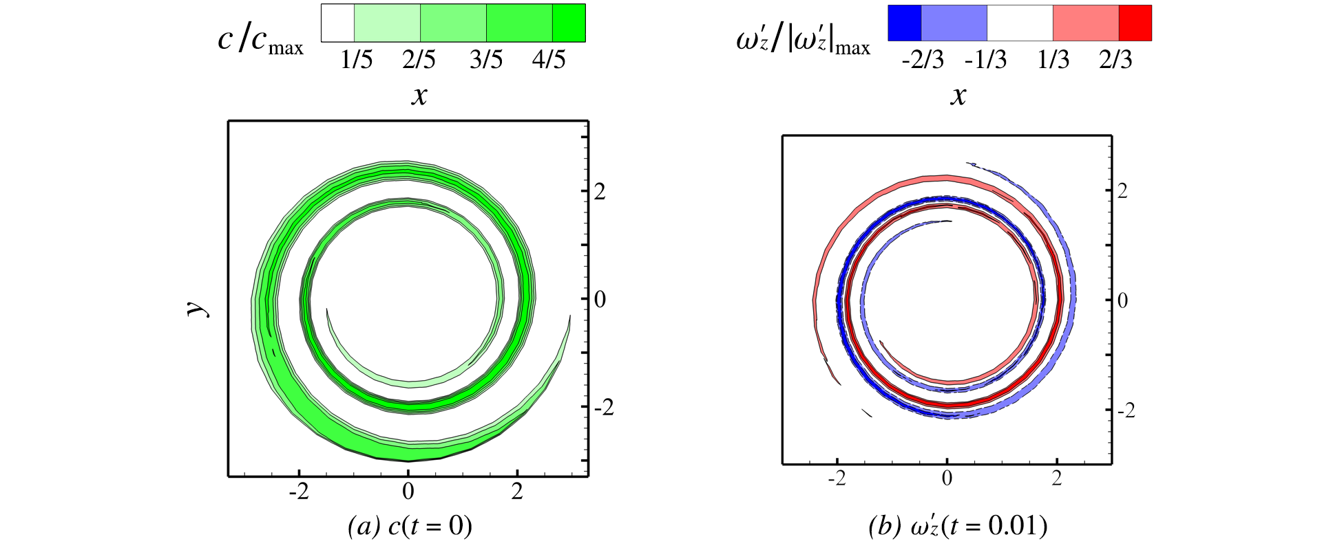
Figure 11: Initiation of optimal transient growth via inertial particles: $(a)$ (left) the initial particle volume fraction contour on the $z=0$ plane, in the pursuit of initiating the perturbation studied in §3.4 (see figure 7), and $(b)$ (right) the axial vorticity perturbation contour on the $z=0$ plane after a brief advancement in time ($t=0.01$) in the two-way coupled vortex-particle simulation solving (4.1) and (4.2) with the initial particle volumetric loading level of $c_{\max}=10^{-6}$. In the right panel, the same contour style as figure 7 is used and $|\omega_{z}^{\prime}(t=0.01)|_{\max}=5.80\times 10^{-6}$.

4.4 Particle-initiated transient growth

Now that the evolution of perturbations of a vortex is governed by (4.4), where the term $(\vartheta-1)c(D\overline{\bm{u}}/Dt)$ serves as a non-zero external force, the overall perturbation dynamics are not only explained by the transient growth process but are also affected by the continual interaction between the particles and the vortex flow (n.b., simliar discussion can be found in Fontane et al., 2008, p. 249). In what follows, we substantiate particle-initiated transient growth by confirming some clear indications of transient growth over short time intervals in the vortex-particle system with the initial particle distribution given in figure 11.

Temporal changes in perturbation energy are displayed in figure 12 with four different levels of particle volumetric loading: $c_{\max}=10^{-4}$, $10^{-5}$, $10^{-6}$, and $10^{-7}$. The case of $c_{\max}=10^{-4}$ is considered to be the upper limit of having $(\vartheta-1)c$ significantly less than order unity (n.b., $\vartheta=10^{3}$). All energy curves follow an almost identical trend, indicating that the same general dynamics take control of these cases. In the right panel of the figure, the data are normalised by the perturbation energy at $t=10$ for each case (note that $E(0)$ is zero and the energy growth we have used, $E(t)/E(0)$, is undefined here) to compare energy amplification between these cases. Overall, the energy amplification in the end appears to be levelled at around $10^{2}$ times $E(10)$ due to the long-time response of the vortex to the particles. Arguably, the amplification above this level should be attributed to the transient growth process, especially including the energy amplification ‘hump’ up to $t=80$. Also, the peak of this hump at $t=50$ coincides with the optimal transient growth period $\tau=50$ that we intend to induce, which we believe strengthens our argument.

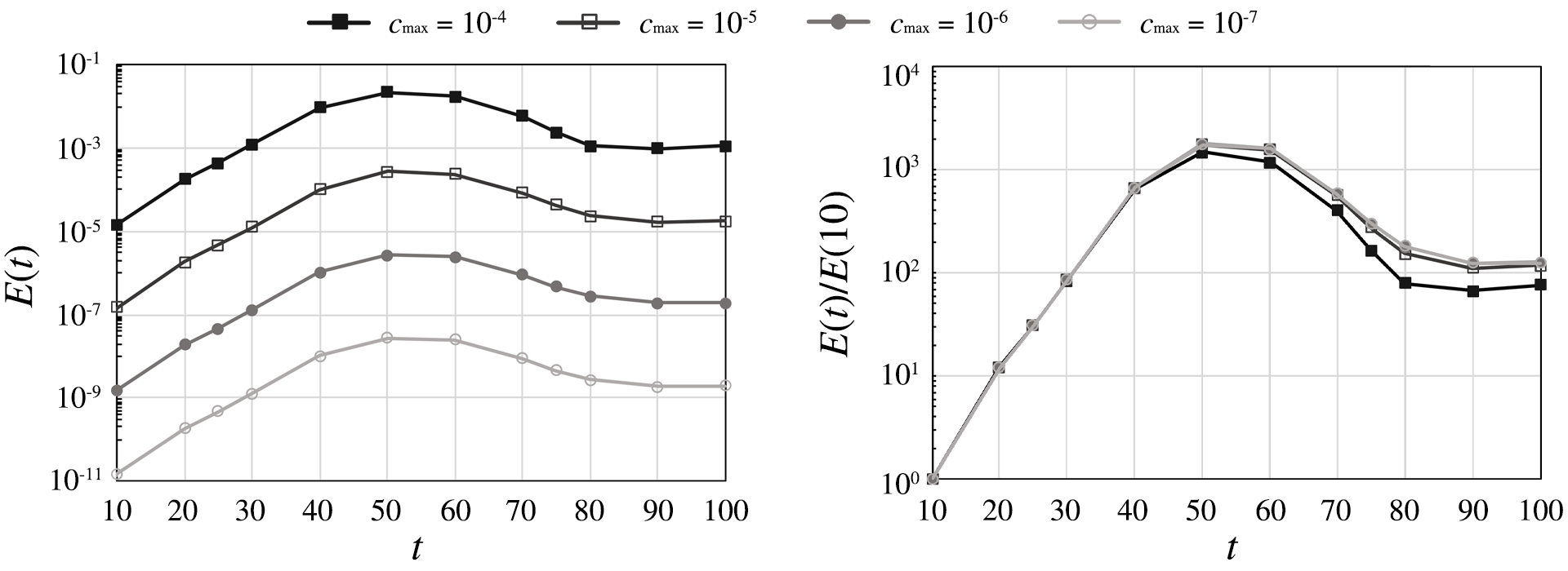
Figure 12: (Left) temporal perturbation energy changes in the vortex-particle motion (see figure 11 for the initial setup) with various particle volumetric loading levels: $c_{\max}=10^{-4}$, $10^{-5}$, $10^{-6}$ and $10^{-7}$ and (right) the same data but normalised by $E(10)$ to compare energy amplification. Note that $E(10)$ is arbitrarily chosen as $E(t)/E(0)$ is undefined in these cases because $E(0)=0$.

Another indication of the particle-initiated transient growth is observed in the evolution of the perturbation structure. In figure 13, the axial vorticity perturbation contours on the $z=0$ plane at $t=25$, $t=50$ and $t=100$ in the vortex-particle simulation with $c_{\max}=10^{-4}$ are depicted. We compare these snapshots with those of the optimally perturbed non-linear vortex growth in figure 9$(c)$. The continual vortex-particle interactions produce the structural discrepancy of the perturbation; this is clearly discernible at $t=100$, where the strong spiraling arms are formed at the periphery as a result of the long-term drag momentum exchange. Nonetheless, in the light of the early-stage perturbation growth until $t=50$, some crucial features representing the optimal transient growth process can be identified, such as the appearance of two weak spiraling arms at the periphery of the core at $t=25$. Most importantly, at the time of the maximum energy growth ($t=50$), the perturbation energy transfer from the periphery to the core — the iconic feature of the optimal transient growth process with respect to $m=1$ — is identifiable. We believe that this serves as the plausible evidence that nearly optimal transient growth takes place via vortex-particle interactions.

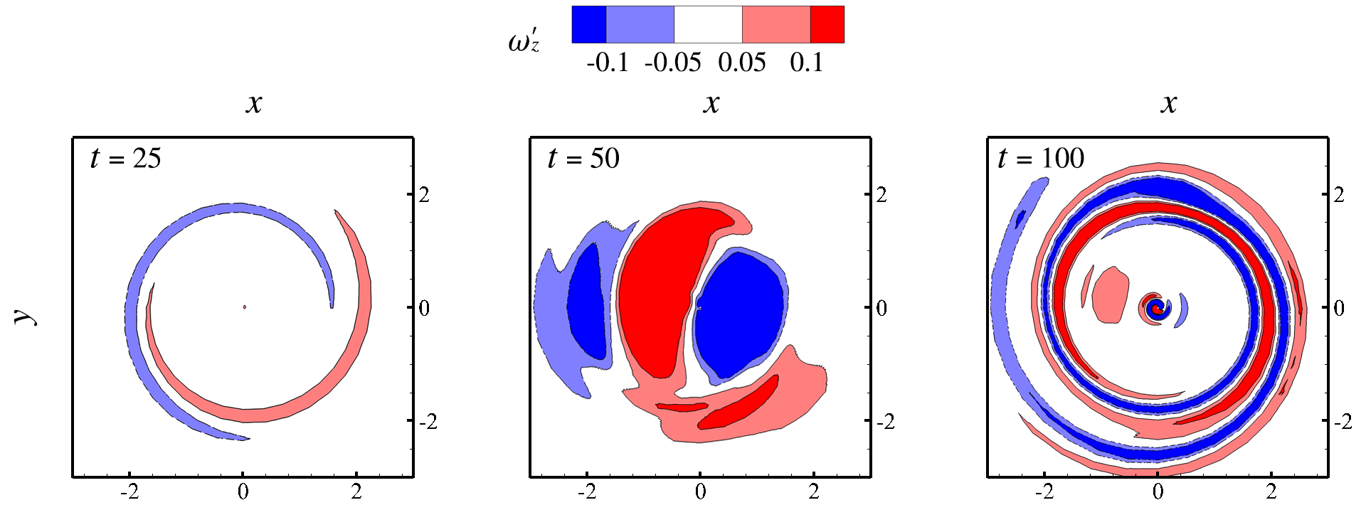
Figure 13: Axial vorticity perturbation contours of the vortex interacting with the peripherially located particles (refer to figure 11 for the illustration of the initial particle distribution) on the $z=0$ plane at $t=25$, $t=50$ and $t=100$. Here, depicted is the case of $c_{\max}=10^{-4}$.

Lastly, we report the transient development of the particle distribution in association with the vortex transient growth. In figure 14, the vortex interacting with the particles where $c_{\max}=10^{-4}$ is visualised using the $\lambda_{2}$-isosurface for the vortex core and the isosurface of 20 % of $c_{\max}$ for the particles. While the vortex evolves into the most excited state ($t=50$) from the unperturbed state ($t=0$), the particles tend to be less dispersed, forming a coherent helical structure that encompasses the vortex core. However, the coherence remains evanescent and dissolves quickly after the maximum perturbation growth at $t=50$. The physical implication of such a temporary increase in coherence, as well as whether it is not just the special case for $m=1$, should be investigated further. For now, we note that the physical phenomenon relevant to the current exemplary case, vortex meandering, is known to have a particular tendency of increasing the ‘orderliness’ of the system (i.e., reduction of the number of dynamically active proper orthogonal decomposition (POD) modes), according to Bölle (2021); the coherence of the particles during the vortex’s transient growth is likely to be correlated with this tendency.

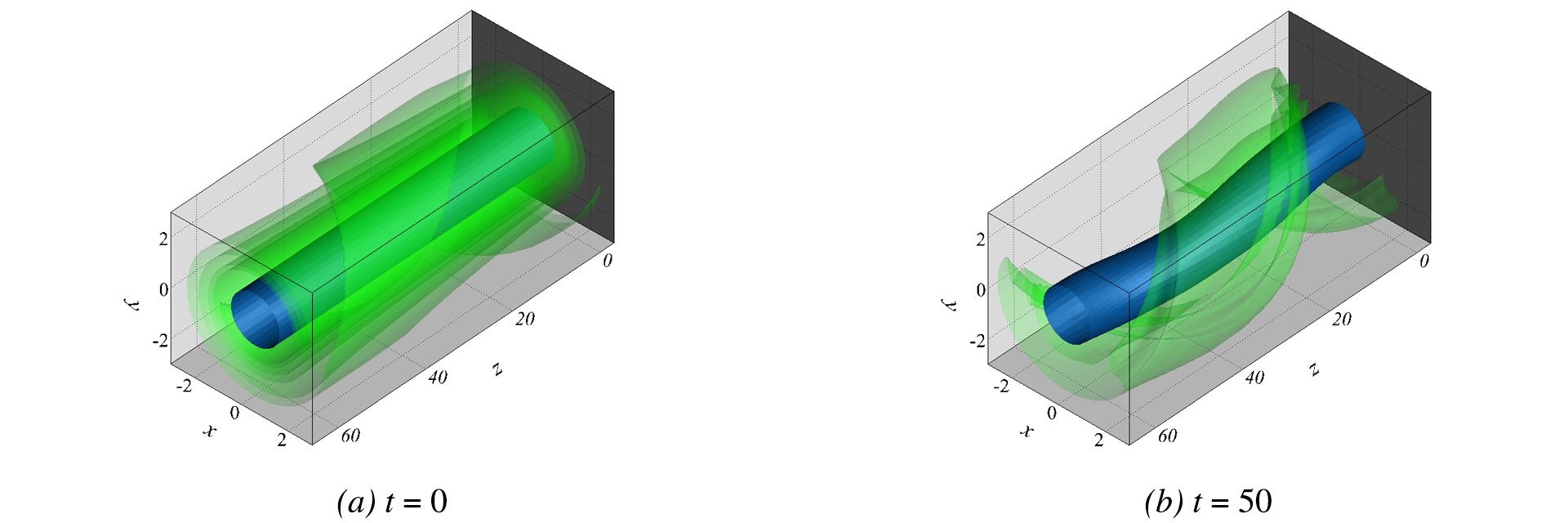
Figure 14: Three-dimensional illustration of the $q$-vortex interacting with the peripherally located particles (see figure 11) of the initial particle volumetric loading level of $c_{\max}=10^{-4}$: $(a)$ $t=0$, and $(b)$ $t=50$. The vortex core is detected using the $\lambda_{2}$-isosurface where $\lambda_{2}=-0.05$, as with figure 10. The green isosurface of $c=2\times 10^{-5}$ (20 % of $c_{\max}$) is drawn together to visualise the particle distribution at each time.

5 Conclusion

In this study, we examined the transient dynamics of a wake vortex using a spectral method tailored to a radially unbounded domain, leading us to confirm that the essential contributor to optimal transient growth among continuous eigenmode families is the viscous critical-layer eigenmode family, rather than the potential eigenmode family. In addition, we explored inertial particles at the periphery of a vortex, motivated by ice crystals forming contrails in the real world, as a significant means of initiating optimal transient growth through drag momentum exchange that has often been neglected.

Using the spectral method for an unbounded domain, which we developed using the mapped Legendre functions as basis functions (see Lee & Marcus, 2023), we numerically analysed the transient growth process of the $q$-vortex slightly disturbed by a perturbation in the form of a sum of well-resolved eigenmodes. In a numerical sense, our method is not vulnerable to some critical issues that unfavorably affect the numerical sensitivity with regard to transient growth analysis, usually found in the conventional spectral method involving Chebyshev polynomials with domain truncation. These issues include the excessive spawning of unnecessary (non-regular or spurious) eigenmode families and the unclear distinction of the viscous critical-layer spectrum from the potential spectrum, due to the incomplete mimicking of the unbounded domain setup. Our method was found to prevent these problems in a proactive manner and, consequently, provide more tolerance for tuning numerical resolution using the map parameter $L$.

Following the typical transient growth formalism, we treated perturbations as a sum of eigenmodes. We then naturally investigated which family of eigenmodes contributes dominantly to optimal perturbations for achieving optimal transient growth. The important behaviour of short-term perturbation energy growth is known to be associated with continuously varying eigenmodes, grounded upon the non-normality of the linearised Navier-Stokes operator. Mao & Sherwin (2012) showed the predominance of continuous eigenmodes in optimal perturbations for the transient growth of a wake vortex, while not providing further categorisation of the continuous eigenmodes, especially for the viscous critical-layer eigenmode family. Through the exploration of the sub-eigenspaces, each respectively spanned by a distinct eigenmode family, it was corroborated that optimal transient growth is principally attributed to the viscous critical-layer eigenmodes. We believe that this finding provides a better alignment of the theoretical foundation of transient growth with the critical layer analysis, rather than the wave packet pseudomode analysis, in compliance with the argument relating inviscid continuous spectrum (CS) transients to vortex growth over short time intervals (Heaton, 2007b). Also, this helps us narrow down our focus when exploring the continuous spectra, as the viscous critical-layer spectrum solely accounts for continuous curves neighbouring the discrete spectrum, whereas the remaining continuous spectrum (potential spectrum) fills an extensive area in the left half of the complex eigenvalue plane.

The energy growth curves and the associated optimal perturbation structures acquired in the present analysis, concerning the axisymmetric ($m=0$) and helical ($m=1$) cases with axial wavenumbers $\kappa$ of order unity or less, were found to be in agreement with previous literature. Overall, we revealed the generic responses during the optimal transient growth process: for $m=0$, the transition of the azimuthal velocity to the other components in consistent ring streaks, and for $m=1$, the transition of the swirling velocity layers outside the vortex core to the large transverse motion in the core. These processes are consistent with those unraveled by previous vortex transient growth studies such as Pradeep & Hussain (2006); Fontane et al. (2008); Mao & Sherwin (2012). In the nonlinear simulations of the $q$-vortex initially with an $(m,\,\kappa)=(1,\,0.1)$ optimal perturbation given the optimal growth period of $\tau=50$, we were able to assert the prevalence of the dynamics of transient growth, particularly until the expected time of maximum energy growth ($t\leq\tau=50$), concluding that these processes predicted by the linearised system are robust even in the original nonlinear system over meaningful time intervals.

Lastly, we discussed the initiation process of transient growth (i.e., generating perturbations from physical interactions, rather than naively assuming their presence at the beginning) and studied the validity of our discussion. Instead of ambient turbulence, which may provide a compelling path for initiation yet is difficult to model precisely due to its fundamental intricacy, we considered vortex-particle interactions inspired by ice crystals, or contrails, in association with aircraft wake vortices in practice. Despite the small size of individual particles, often leading to the assumption that their backward influence on the flow is negligible, their bulk inertial effect along with the large particle number density might make them not simply neglected. Enabling the two-way coupling between the particles and the vortex flow via drag momentum exchange, we ran the vortex-particle simulations with the particles initially distributed at the periphery of the vortex core, in order to initiate the optimal perturbation for $(m,\,\kappa)=(1,\,0.1)$ studied ahead. We successfully spotted clear indications of optimal transient growth during the continual vortex-particle interactions, including the large energy amplification hump that peaks at $t=\tau=50$ and the perturbation energy transfer process from the periphery into the core.

The present study underscores the significance of the optimal transient growth process of a single vortex over short time intervals, initially structured by the critical-layer eigenmodes. The initiation of transient growth via particle drag not only demonstrates the practicability of the transient growth process but also reaffirms the susceptibility of the vortex motion, even against physical interactions that have often been neglected either for simplicity or due to superficial insignificance. As Fontane et al. (2008) suggested in their vortex transient growth study with stochastic forcing, the transient growth process might be active regardless of the details or dynamics of the perturbations; particle drag could be one of those activators. Even though our motivation for considering particles was founded upon existing contrails, particles as a means of perturbing a vortex can be more useful if we attempt to actively control the wake vortex system to expedite its destabilisation, beyond understanding its nature, through, for example, deliberate injection of inertial particles. Leveraging the same numerical scheme (see Appendix B), we expect to expand our scope to the analysis of a vortex pair or multi-vortex system to investigate whether an individual vortex’s transient growth accelerates practical and well-known instabilities in aircraft wake vortices, such as the Crow instability, for expeditous destabilisation.

[Acknowledgements]We would like to thank Dr. Joseph A. Barranco (San Francisco State University) for sharing insights about particle-laden flow simulations using the fast equilibirum assumption, and Jinge Wang (University of California, Berkeley) for providing discussions with respect to wake vortex instabilities.

[Funding]This research received no specific grant from any funding agency, commercial or not-for-profit sectors.

[Declaration of interests]The authors report no conflict of interest.

Appendix A Numerical integration for energy calculation

Consider the following definite integral $I$ of an arbitrary scalar $f$ in terms of $r$:

$$I(f)\equiv\int_{0}^{\infty}{f^{*}(r)f(r)rdr}.$$ (A.1)

It is assumed that $f$ decays sufficiently fast as $r\rightarrow\infty$ so that $I(f)$ is well-defined. Using change of variables from $r\in\left[0,\infty\right)$ to a new variable $\zeta\in[-1,1)$ via

$$\zeta\equiv\frac{r^{2}-L^{2}}{r^{2}+L^{2}},$$ (A.2)

where $L>0$ is the map parameter, we alter (A.1) into a new form as follows:

$$I(f)=\int_{-1}^{1}{f^{*}\left(L\sqrt{\frac{1+\zeta}{1-\zeta}}\right)f\left(L\sqrt{\frac{1+\zeta}{1-\zeta}}\right)\frac{L^{2}}{(1-\zeta)^{2}}d\zeta}.$$ (A.3)

Applying the Gauss-Legendre quadrature rule as used by Lee & Marcus (2023, p. 13), we obtain the numerical form of (A.3) as

$$I(f)\simeq\sum_{j=1}^{N}f^{*}(r_{j})\frac{L^{2}\varpi_{j}}{(1-\zeta_{j})^{2}}f(r_{j}),$$ (A.4)

where $\zeta_{j}$ and $\varpi_{j}$ are the $j$th abscissa and the $j$th weight of the Gauss-Legendre quadrature rule for degree $N$ $(j=1,~{}2,\cdots,~{}N)$, and $r_{j}\equiv L\sqrt{(1+\zeta_{j})/(1-\zeta_{j})}$ is the $j$th radial collocation point. Note that (A.4) can be expressed as $\bm{f}^{*}\mathsfbi{M}^{{\ddagger}}\bm{f}$ if we define $\bm{f}$ as the discretised version of $f$ in physical space, i.e., $\bm{f}\equiv\left(f(r_{1}),~{}\cdots,~{}f(r_{N})\right)$ and $\mathsfbi{M}^{{\ddagger}}$ as

$$\mathsfbi{M}^{{\ddagger}}\equiv\text{diag}\left(\frac{L^{2}\varpi_{1}}{(1-\zeta_{1})^{2}},~{}\cdots,~{}\frac{L^{2}\varpi_{N}}{(1-\zeta_{N})^{2}}\right).$$ (A.5)

Finally, the energy in (2.7), which is equal to $I(\tilde{\bm{u}}_{r})+I(\tilde{\bm{u}}_{\phi})+I(\tilde{\bm{u}}_{z})$, can be numerically calculated as follows:

$$E(\tilde{\bm{u}})=\underbrace{\left(\begin{array}[]{c;{2pt/1pt}c;{2pt/1pt}c}\tilde{\bm{\upsilon}}_{r}^{*}&\tilde{\bm{\upsilon}}_\phi^*&\tilde{\bm{\upsilon}}_z^*\end{array}\right)}_{\tilde{\bm{\upsilon}}^{*}}\underbrace{\left(\begin{array}[]{c;{2pt/1pt}c;{2pt/1pt}c}\mathsfbi{M}^{{\ddagger}}&\mathsfbi{0}&\mathsfbi{0}\\[2.0pt] \hdashline[2pt/1pt]\mathsfbi{0}&\mathsfbi{M}^{\textdaggerdbl}&\mathsfbi{0}\\[2.0pt] \hdashline[2pt/1pt]\mathsfbi{0}&\mathsfbi{0}&\mathsfbi{M}^{\textdaggerdbl}\end{array}\right)}_{\mathsfbi{M}}\underbrace{\left(\begin{array}[]{c}\tilde{\bm{\upsilon}}_{r}\\[2.0pt] \hdashline[2pt/1pt]\tilde{\bm{\upsilon}}_{\phi}\\[2.0pt] \hdashline[2pt/1pt]\tilde{\bm{\upsilon}}_{z}\end{array}\right)}_{\tilde{\bm{\upsilon}}}.$$ (A.6)

This constitutes the formation of $\mathsfbi{M}$ representing the matrix calculation for energy in (2.8).

Appendix B Numerical setup for non-linear simulations

To discretise the radially unbounded domain considered in this paper, especially in three dimensions for non-linear simulations, we employ a pseudo-spectral method based on the mapped Legendre spectral collocation method. The method assumes an arbitrary scalar field (or a component of an arbitrary vector field) that decays fast and harmonically in $r$, say, $f$, to be expanded as follows:

$$f(r,\phi,z,t)=\sum_{n=|m|}^{\infty}\sum_{m=-\infty}^{\infty}\sum_{k=-\infty}^{\infty}f_{nmk}(t)P_{L_{n}}^{m}(r)e^{im\phi}e^{ik\frac{2\pi}{Z}z},$$ (B.1)

where $Z$ is the computational domain length in the $z$ direction, corresponding to the longest axial wavelength under consideration. The expansion assumes periodicity with a period of $Z$ in $z$ and ensures analyticity at $r=0$ and harmonic decay at radial infinity, thanks to the mapped Legendre basis functions $P_{L_{n}}^{m}(r)$. In this study, we chose $Z=20\pi$, standing for the smallest axial wavenumber of $0.1$ to be considered. On the other hand, $L$, the map parameter, defines the high-resolution region during pseudo-spectral calculations to be $0\leq r<L$ (see Lee & Marcus, 2023, p. 13), and we chose $L=4$ to secure resolution for the vortex motion of the core and the near periphery.

Although special logarithmic terms may be required to account for the $O(1/r)$ decay at large $r$ (see Matsushima & Marcus, 1997, p. 331), we omit them here for simplicity in description. It is noted that the method was initially introduced by Matsushima & Marcus (1997) with several validation examples involving the vorticity equations, where one may look for additional details. Also, a more in-depth discussion of the implementation of the method in vortex stability research can be found in Lee & Marcus (2023).

The set of the coefficients $f_{nmk}$ now represents $f$ in a discrete manner. As practical computations demand the set to be finite, we chose $n\leq 400$, $|m|\leq 16$, and $|k|\leq 16$. The reason the radial elements make use of an extra degree (i.e., large $n$) compared to the others is to cope with the viscous critical layers of radially fine structures at high $\Rey$. Otherwise, for the purpose of our computations, a high degree for the other elements (i.e., large $m$ and $k$) is not necessary, as our focus is principally on small wavenumbers.

In pure vortex simulations (without particles), we consider the toroidal and poloidal streamfunctions $\psi$ and $\chi$ as the state variables to be discretised in space (by applying the toroidal-poloidal decomposition, $\mathbb{P}$, to the momentum equation) and then integrate them in time to solve the vortex motion. With particles, the particle volume fraction $c$ is additionally considered, coupling the vortex and particle motions. When it comes to time integration, the fractional step method is employed, utilising the Adams-Bashforth method for non-linear terms (e.g., advection) and the Crank-Nicholson method for linear terms (e.g., dissipation) with Richardson extrapolation for the first time step (see Matsushima & Marcus, 1997, p. 343). Throughout preliminary simulations with the $q$-vortex ($q=4$) perturbed with a small-amplitude eigenmode with a known frequency and decay rate, the time step was set to $10^{-3}$ as it yielded a tolerable error during the time integration between $t=0$ and $t=100$.

References

- Antkowiak & Brancher (2004) Antkowiak, A. & Brancher, P. 2004 Transient energy growth for the Lamb–Oseen vortex. Physics of Fluids 16 (1), L1–l4.
- Ash & Khorrami (1995) Ash, R. L. & Khorrami, M. R. 1995 Vortex stability. In Fluid Vortices (ed. S. I. Green), pp. 317–372. Dordrecht, NL: Springer Netherlands.
- Auton et al. (1988) Auton, T. R., Hunt, J. C. R. & Prud’Homme, M. 1988 The force exerted on a body in inviscid unsteady non-uniform rotational flow. Journal of Fluid Mechanics 197, 241–257.
- Batchelor (1964) Batchelor, G. K. 1964 Axial flow in trailing line vortices. Journal of Fluid Mechanics 20 (4), 645–658.
- Bölle (2021) Bölle, T. 2021 Treatise on the meandering of vortices. PhD thesis, Institut Polytechnique de Paris.
- Bölle et al. (2023) Bölle, T., Brion, V., Couliou, M. & Molton, P. 2023 Experiment on jet-vortex interaction for variable mutual spacing. Physics of Fluids 35, 015117.
- Crow (1970) Crow, S. C. 1970 Stability theory for a pair of trailing vortices. AIAA Journal 8 (12), 2172–2179.
- Crow & Bate (1976) Crow, S. C. & Bate, E. R. 1976 Lifespan of trailing vortices in a turbulent atmosphere. Journal of Aircraft 13 (7), 476–482.
- Devenport et al. (1997) Devenport, W. J., Zsoldos, J. S. & Vogel, C. M. 1997 The structure and development of a counter-rotating wing-tip vortex pair. Journal of Fluid Mechanics 332 (1997), 71–104.
- Edstrand et al. (2016) Edstrand, A. M., Davis, T. B., Schmid, P. J., Taira, K. & Cattafesta, L. N. 2016 On the mechanism of trailing vortex wandering. Journal of Fluid Mechanics 801, R1.
- El-Ramly & Rainbird (1977) El-Ramly, Z. & Rainbird, W. J. 1977 Effect of simulated jet engines on the flowfield behind a swept-back wing. Journal of Aircraft 14 (4), 343–349.
- Fabre & Jacquin (2004) Fabre, D. & Jacquin, L. 2004 Viscous instabilities in trailing vortices at large swirl numbers. Journal of Fluid Mechanics 500, 239–262.
- Ferry & Balachandar (2001) Ferry, J. & Balachandar, S. 2001 A fast Eulerian method for disperse two-phase flow. International Journal of Multiphase Flow 27 (7), 1199–1226.
- Fontane et al. (2008) Fontane, J., Brancher, P. & Fabre, D. 2008 Stochastic forcing of the Lamb-Oseen vortex. Journal of Fluid Mechanics 613, 233–254.
- Hallock & Holzäpfel (2018) Hallock, J. N. & Holzäpfel, F. 2018 A review of recent wake vortex research for increasing airport capacity. Progress in Aerospace Sciences 98, 27–36.
- Han et al. (2000) Han, J., Lin, Y.-L., Schowalter, D. G., Arya, S. P. & Proctor, F. H. 2000 Within homogeneous turbulence: Crow instability large eddy simulation of aircraft wake vortices. AIAA Journal 38 (2), 292–300.
- Heaton (2007a) Heaton, C. J. 2007a Centre modes in inviscid swirling flows and their application to the stability of the Batchelor vortex. Journal of Fluid Mechanics 576, 325–348.
- Heaton (2007b) Heaton, C. J. 2007b Optimal growth of the Batchelor vortex viscous modes. Journal of Fluid Mechanics 592, 495–505.
- Heaton & Peake (2007) Heaton, C. J. & Peake, N. 2007 Transient growth in vortices with axial flow. Journal of Fluid Mechanics 587, 271–301.
- Jeong & Hussain (1995) Jeong, J. & Hussain, F. 1995 On the identification of a vortex. Journal of Fluid Mechanics 285, 69–94.
- Kärcher (2018) Kärcher, B. 2018 Formation and radiative forcing of contrail cirrus. Nature Communications 9, 1824.
- Kärcher et al. (1996) Kärcher, B., Peter, T., Biermann, U. M. & Schumann, U. 1996 The initial composition of jet condensation trails. Journal of the Atmospheric Sciences 53 (21), 3066–3083.
- Khorrami (1991) Khorrami, M. R. 1991 On the viscous modes of instability of a trailing line vortex. Journal of Fluid Mechanics 225, 197–212.
- Khorrami et al. (1989) Khorrami, M. R., Malik, M. R. & Ash, R. L. 1989 Application of spectral collocation techniques to the stability of swirling flows. Journal of Computational Physics 81 (1), 206–229.
- Le Dizès (2004) Le Dizès, S. 2004 Viscous critical-layer analysis of vortex normal modes. Studies in Applied Mathematics 112 (4), 315–332.
- Lee et al. (2021) Lee, D. S., Fahey, D. W., Skowron, A., Allen, M. R., Burkhardt, U., Chen, Q., Doherty, S. J., Freeman, S., Forster, P. M., Fuglestvedt, J., Gettelman, A., De León, R. R., Lim, L. L., Lund, M. T., Millar, R. J., Owen, B., Penner, J. E., Pitari, G., Prather, M. J., Sausen, R. & Wilcox, L. J. 2021 The contribution of global aviation to anthropogenic climate forcing for 2000 to 2018. Atmospheric Environment 244, 117834.
- Lee & Marcus (2023) Lee, S. & Marcus, P. S. 2023 Linear stability analysis of wake vortices by a spectral method using mapped Legendre functions. Journal of Fluid Mechanics 967, A2.
- Leibovich (1978) Leibovich, S. 1978 The Structure of Vortex Breakdown. Annual Review of Fluid Mechanics 10, 221–246.
- Leibovich & Stewartson (1983) Leibovich, S. & Stewartson, K. 1983 A sufficient condition for the instability of columnar vortices. Journal of Fluid Mechanics 126, 335–356.
- Lessen et al. (1974) Lessen, M., Singh, P. J. & Paillet, F. 1974 The stability of a trailing line vortex. Part 1. Inviscid theory. Journal of Fluid Mechanics 63 (4), 753–763.
- Lewellen & Lewellen (2001) Lewellen, D. C. & Lewellen, W. S. 2001 The effects of aircraft wake dynamics on contrail development. Journal of the Atmospheric Sciences 58 (4), 390–406.
- Lin (1955) Lin, C.-C. 1955 The Theory of Hydrodynamic Stability, 1st edn. Cambridge, UK: Cambridge University Press.
- Mahalov (1993) Mahalov, A. 1993 The instability of rotating fluid columns subjected to a weak external Coriolis force. Physics of Fluids A: Fluid Dynamics 5 (4), 891–900.
- Mao & Sherwin (2011) Mao, X. & Sherwin, S. 2011 Continuous spectra of the Batchelor vortex. Journal of Fluid Mechanics 681, 1–23.
- Mao & Sherwin (2012) Mao, X. & Sherwin, S. J. 2012 Transient growth associated with continuous spectra of the Batchelor vortex. Journal of Fluid Mechanics 697, 35–59.
- Matsushima & Marcus (1997) Matsushima, T. & Marcus, P. S. 1997 A spectral method for unbounded domains. Journal of Computational Physics 137 (2), 321–345.
- Maxey & Riley (1983) Maxey, M. R. & Riley, J. J. 1983 Equation of motion for a small rigid sphere in a nonuniform flow. Physics of Fluids 26 (4), 883–889.
- Moore & Saffman (1975) Moore, D. W. & Saffman, P. G. 1975 The instability of a straight vortex filament in a strain field. Proceedings of the Royal Society of London. A. Mathematical and Physical Sciences 346 (1646), 413–425.
- Muthiah & Samanta (2018) Muthiah, G. & Samanta, A. 2018 Transient energy growth of a swirling jet with vortex breakdown. Journal of Fluid Mechanics 856, 288–322.
- Naiman et al. (2011) Naiman, A. D., Lele, S. K. & Jacobson, M. Z. 2011 Large eddy simulations of contrail development: Sensitivity to initial and ambient conditions over first twenty minutes. Journal of Geophysical Research: Atmospheres 116, D21208.
- Navrose et al. (2018) Navrose, Johnson, H. G., Brion, V., Jacquin, L. & Robinet, J. C. 2018 Optimal perturbation for two-dimensional vortex systems: route to non-axisymmetric state. Journal of Fluid Mechanics 855, 922–952.
- Paoli & Garnier (2005) Paoli, R. & Garnier, F. 2005 Interaction of exhaust jets and aircraft wake vortices: small-scale dynamics and potential microphysical-chemical transformations. Comptes Rendus Physique 6 (4-5), 525–547.
- Paoli et al. (2004) Paoli, R., Hélie, J. & Poinsot, T. 2004 Contrail formation in aircraft wakes. Journal of Fluid Mechanics 502, 361–373.
- Pradeep & Hussain (2006) Pradeep, D. S. & Hussain, F. 2006 Transient growth of perturbations in a vortex column. Journal of Fluid Mechanics 550, 251.
- Proctor et al. (2000) Proctor, F. H., Hamilton, D. W. & Han, J. 2000 Wake vortex transport and decay in ground effect: Vortex linking with the ground, In 38th Aerospace Sciences Meeting and Exhibit, no. AIAA–2000–0757. Reston, VA: American Institute of Aeronautics and Astronautics.
- Sarpkaya (1983) Sarpkaya, T. 1983 Trailing vortices in homogeneous and density-stratified media. Journal of Fluid Mechanics 136, 85–109.
- Schmid & Henningson (1994) Schmid, P. J. & Henningson, D. S. 1994 Optimal energy density growth in Hagen–Poiseuille flow. Journal of Fluid Mechanics 277, 197–225.
- Schmid & Henningson (2001) Schmid, P. J. & Henningson, D. S. 2001 Stability and transition in shear flows, Applied Mathematical Sciences, vol. 142. New York, NY: Springer New York.
- Schumann (2005) Schumann, U. 2005 Formation, properties and climatic effects of contrails. Comptes Rendus Physique 6, 549–565.
- Shirgaonkar & Lele (2004) Shirgaonkar, A. A. & Lele, S. K. 2004 Large eddy simulation of early stage aircraft contrails. Tech. Rep.. Stanford University, Stanford, CA.
- Shuai et al. (2022) Shuai, S., Jeswin Dhas, D., Roy, A. & Kasbaoui, M. H. 2022 Instability of a dusty vortex. Journal of Fluid Mechanics 948, A56.
- Shuai & Kasbaoui (2022) Shuai, S. & Kasbaoui, M. H. 2022 Accelerated decay of a Lamb–Oseen vortex tube laden with inertial particles in Eulerian–Lagrangian simulations. Journal of Fluid Mechanics 936, A8.
- Spalart (1998) Spalart, P. R. 1998 Airplane trailing vortices. Annual Review of Fluid Mechanics 30, 107–138.
- Stewartson & Brown (1985) Stewartson, K. & Brown, S. N. 1985 Near-neutral centre-modes as inviscid perturbations to a trailing line vortex. Journal of Fluid Mechanics 156, 387.
- Trefethen & Embree (2005) Trefethen, L. N & Embree, M. 2005 Spectra and pseudospectra: the behavior of nonnormal matrices and operators. Princeton, NJ: Princeton University Press.
- Tsai & Widnall (1976) Tsai, C.-Y. & Widnall, S. E. 1976 The stability of short waves on a straight vortex filament in a weak externally imposed strain field. Journal of Fluid Mechanics 73 (4), 721–733.
- Voigt et al. (2011) Voigt, C., Schumann, U., Jessberger, P., Jurkat, T., Petzold, A., Gayet, J.-F., Krämer, M., Thornberry, T. & Fahey, D. W. 2011 Extinction and optical depth of contrails. Geophysical Research Letters 38 (11), L11806.
- Wang et al. (2024) Wang, J., Lee, S. & Marcus, P. S. 2024 Triadic resonance in columnar vortices, arXiv: 2402.05287.