Fourth-order modon in a rotating self-gravitating fluid

Abstract

We present a two-dimensional nonlinear equation to govern the dynamics of disturbances in a rotating self-gravitating fluid. The nonlinear term of the equation has the form of a Poisson bracket (Jacobian), and the linear part contains, along with the Laplacian, a biharmonic operator. A solution was found in the form of a dipole vortex (modon). The solution and all its derivatives up to the fourth order are continuous on the separatrix.

I Introduction

The dynamics of self-gravitating systems (within the framework of Newtonian theory) was first studied by Jeans Jeans1929 , where the instability of disturbances with wavelengths greater than the so-called Jeans wavelength $\lambda_{J}$ was predicted. It is believed that the Jeans instability is the source of the emergence of large-scale structures in the Universe, and this problem remains one of the most challenging in astrophysics. The linear theory is valid, however, only for sufficiently small (strictly speaking, infinitesimal) amplitudes of disturbances, when nonlinear effects can be neglected. Nonlinear coherent structures, such as solitons and vortices, in self-gravitating fluids have been considered in a number of works. One-dimensional solitons in such systems were studied in Mikhailovskii1977 ; Yueh1981 ; Ono1994 ; Zhang1995 ; Zhang1998 ; Gotz1988 ; Adams1994 ; Semelin2001 ; Verheest1997 ; Masood2010 ; Verheest2005 , and multidimensional structures were discussed in Fridman1991 ; Jovanovich1990 ; Shukla1993 ; Zinzadze2000 ; Pokhotelov1998 ; Shukla1995 ; Abrahamyan2020 ; Lashkin2023 . In a broad sense, a soliton is a localized structure (not necessarily one-dimensional) resulting from the balance of dispersion and nonlinearity effects. Multidimensional solitons often turn out to be unstable, and the most well-known phenomena in this case are wave collapse and wave breaking Kuznetsov1986 ; KuznetsovZakharov2000 ; Zakharov_UFN2012 . The two-dimensional (2D) and three-dimensional (3D) structures in Fridman1991 ; Jovanovich1990 ; Shukla1993 ; Zinzadze2000 ; Pokhotelov1998 ; Shukla1995 ; Abrahamyan2020 ; Lashkin2023 were considered under the assumption that the characteristic frequencies are much lower than the rotation frequency of the self-gravitating fluid. In geophysics, this corresponds to the quasi-geostrophic approximation Pedlosky1987 . In particular, in Fridman1991 a nonlinear equation governing the dynamics of finite amplitude disturbances in a rotating self-gravitating gas was obtained, and this equation is completely similar to the well-known Charney equation in geophysics Charney1948 for nonlinear Rossby waves in atmospheres of rotating planets and in oceans (in plasma physics, this equation is known as the Hasegawa-Mima equation Hasegawa1978 , and the rotation frequency is replaced by the ion gyrofrequency in an external magnetic field). The corresponding solution is the 2D Larichev-Reznik dipole vortex in the form of a cyclone-anticyclone pair (also called the Larichev-Reznik modon or Larichev-Reznik soliton) Larichev1976a ; Larichev1976b . The term modon was introduced by Stern Stern1975 to designate a steadily moving localized vortex structure, and is widely used for particular solutions of some type of equations with nonlinearity in the form of Poisson brackets (mainly in geophysics and plasma physics) Flierl1987 ; Petviashvili_book1992 ; Berestov1979 ; Horton1983 ; Swaters1989 ; Ghil2002 ; Kizner2008 ; Zeitlin2022 . A common property of these solutions is the presence of a circular (in the 2D case) or spherical (3D case) cut (the separatrix) with subsequent matching of the solution in the internal and external regions. A remarkable property of the Larichev-Reznik modon is its stability under head-on and overtaking collisions with zero-impact parameter between the modons Flierl1980 ; Makino1981 ; Williams1982 . Recent work Lashkin2017 demonstrated elastic collisions even between the 3D modons for the 3D version of the Hasegawa-Mima equation.

In most works on modons and their generalizations, the linear part of the equations contains derivatives of no higher than second order and, as a consequence, continuity of both the solution itself and its derivatives no higher than the second order is required. A few exceptions are, for example, works Horton1986 ; Lakhin1987 ; Aburdjania1988PhysScr , where solutions in the form of dipole vortices were considered within the framework of a system of two nonlinear equations for two independent scalar functions, which is equivalent to an equation with fourth-order derivatives. In the present paper, for the case of a self-gravitating fluid, we present a nonlinear equation including fourth-order derivatives in the linear part and a nonlinear term in the form of Poisson brackets (Jacobian). We find an analytical solution to this equation in the form of a dipole vortex (modon). The solution and all its derivatives up to the fourth order are continuous on the seperatrix.

The paper is organized as follows. In Sec. II, we present the model equation for the rotating self-gravitating fluid. In Sec. III, an analytical modon solution is found. Section IV concludes the paper.

II Model Equations

We consider a self-gravitating fluid rotating with constant angular velocity $\mathbf{\Omega}_{0}=\Omega_{0}\mathbf{\hat{z}}$ and with an equilibrium density $\rho_{0}$ in the plane perpendicular to the $\mathbf{\hat{z}}$-axis. It is also assumed that the characteristic frequencies of disturbances are small compared to the rotation frequency. A weak inhomogeneity of the equilibrium density in the radial direction with a characteristic inhomogeneity length $L$ (all characteristic scales of perturbations are much larger than $L$) is assumed, and a local Cartesian coordinate system is used ($x$ corresponds to the radial coordinate $r$ and $y$ corresponds to the polar angle $\varphi$). Based on the momentum and continuity fluid equations for the self-gravitating rotating isothermal gas and the Poisson equation for the gravitational potential, the following system of coupled 3D nonlinear equations for the perturbed gravitational potential $\psi$ and the $z$-component of the fluid velocity $v_{z}$ was obtained in a recent paper Lashkin2023 ,

$$\frac{\partial\Phi}{\partial t}-\frac{\omega_{0}^{2}}{2\Omega_{0}L}\frac{\partial\Pi}{\partial y}+\frac{1}{2\Omega_{0}}\{\Pi,\Phi\}+\omega_{0}^{2}\frac{\partial v_{z}}{\partial z}=0,$$ (1)

$$\frac{\partial v_{z}}{\partial t}+\frac{1}{2\Omega_{0}}\left\{\Pi,v_{z}\right\}+\frac{\partial\Pi}{\partial z}=0,$$ (2)

where

$$\Phi=\Delta\psi-\frac{\omega_{0}^{2}}{4\Omega_{0}^{2}}\Delta_{\perp}\Pi,\quad\Pi=\psi+\frac{c_{s}^{2}}{\omega_{0}^{2}}\Delta\psi,$$ (3)

being $\Delta=\partial^{2}/\partial x^{2}+\partial^{2}/\partial y^{2}+\partial^{2}/\partial z^{2}$ and $\Delta_{\perp}=\partial^{2}/\partial x^{2}+\partial^{2}/\partial y^{2}$ are the 3D and 2D (transverse) Laplacian respectively. Here $\omega_{0}$ is the Jeans frequency defined by $\omega_{0}=2\sqrt{\pi G\rho_{0}}$, where $G$ is the gravitational constant, and $c_{s}$ is the speed of sound in an adiabatic medium of uniform density $\rho_{0}$. The nonlinear terms in Eqs. (1) and (2) have been written in the form of the Poisson bracket (Jacobian) defined as

$$\{f,g\}=\frac{\partial f}{\partial x}\frac{\partial g}{\partial y}-\frac{\partial f}{\partial y}\frac{\partial g}{\partial x}.$$ (4)

We consider the 2D case and neglect the motions along the $z$-axis, which is valid provided

$$\frac{\partial/\partial t}{\Omega_{0}}\gg\frac{l_{y}}{l_{z}^{2}}L,$$ (5)

where $l_{y}$ and $l_{z}$ are characteristic lengths of disturbances along the $y$-axis and $z$-axis, respectively. One can verify that this is equivalent to neglecting the interaction with the acoustic wave in Lashkin2023 . From Eqs. (1) and (2) we then obtain one equation for the potential $\psi$,

$$\frac{\partial\Phi}{\partial t}-\frac{\omega_{0}^{2}}{2\Omega_{0}L}\frac{\partial\Pi}{\partial y}+\frac{1}{2\Omega_{0}}\{\Pi,\Phi\}=0,$$ (6)

where in Eq. (3) the 3D Laplacian is replaced by a two-dimensional one, $\Delta\rightarrow\Delta_{\perp}$. In the linear approximation, taking $\psi(\mathbf{r}_{\perp},t)\sim\exp(i\mathbf{k}_{\perp}\cdot\mathbf{r}_{\perp}-i\omega t)$, where $\omega$ and $\mathbf{k}_{\perp}=(k_{x},k_{y})$ are the frequency and transverse wave vector respectively, Eq. (6) yields the dispersion relation

$$\omega=\frac{k_{y}c_{s}^{2}}{2\Omega_{0}L[k^{2}_{\perp}/(k^{2}_{\perp}-k^{2}_{J})+k^{2}_{\perp}c_{s}^{2}/(4\Omega_{0}^{2})]},$$ (7)

where $k_{\perp}^{2}=k_{x}^{2}+k_{y}^{2}$, $k_{J}=1/\lambda_{J}$, and $\lambda_{J}=c_{s}/\omega_{0}$ is the Jeans length. Note that the solution in the form of a monochromatic plane wave is also a solution to Eq. (6) since in this case the nonlinearity in the form of a Poisson bracket vanishes identically. Introducing the variables $t^{{}^{\prime}}$, $\mathbf{r}_{\perp}^{{}^{\prime}}$, and $\psi^{{}^{\prime}}$ by

$$t=\frac{t^{\prime}}{2\Omega_{0}},\quad\mathbf{r}_{\perp}=\lambda_{J}\mathbf{r}_{\perp}^{\prime},\quad\psi=\frac{4\Omega_{0}^{2}c_{s}^{2}}{\omega_{0}^{2}}\psi^{\prime},$$ (8)

we rewrite Eq. (6) in the dimensionless form (primes have been omitted),

$$\frac{\partial}{\partial t}(\alpha\Delta_{\perp}\psi-\Delta_{\perp}^{2}\psi)-v_{\ast}\frac{\partial}{\partial y}(\psi+\Delta_{\perp}\psi)$$

$$+\{\psi+\Delta_{\perp}\psi,\alpha\Delta_{\perp}\psi-\Delta_{\perp}^{2}\psi\}=0,$$ (9)

where $\alpha=4\Omega_{0}^{2}/\omega_{0}^{2}-1$, and $v_{\ast}=\lambda_{J}/L$. Note that our basic equation (9) contains a biharmonic operator, that is, in particular, fourth-order spatial derivatives. Equation (9) can be written as

$$\frac{\partial\Gamma}{\partial t}+\{\psi+\Delta_{\perp}\psi,\Gamma\}=0,$$ (10)

where $\Gamma=\Delta_{\perp}^{2}\psi-\alpha\Delta_{\perp}\psi-v_{\ast}x$ can be treated as a generalized vorticity, and then Eq. (10) describes the generalized vorticity convection in an incompressible velocity field $\mathbf{v}_{D}=[\hat{\mathbf{z}}\times\nabla_{\perp}(\psi+\Delta_{\perp}\psi)]$ with $d\Gamma/dt=0$, where $d/dt=\partial/\partial t+\mathbf{v}_{D}\cdot\nabla_{\perp}$ is the convective derivative. Conservation of the generalized vorticity $\Gamma$ along the streamlines implies that Eq. (9) has an infinite set of integrals of motion (the so called Casimir invariants),

$$\int f(\Gamma)\,d^{2}\mathbf{r},$$ (11)

where $f$ is an arbitrary function. Other integrals of motion are

$$\int(\psi+\Delta_{\perp}\psi)\Gamma\,d^{2}\mathbf{r},\quad\int x\Gamma\,d^{2}\mathbf{r},\quad\int(y+v_{\ast}t)\Gamma\,d^{2}\mathbf{r}.$$ (12)

III Modon solution

We look for stationary traveling wave solutions of Eq. (10) of the form

$$\psi(x,y,t)=\psi(x,y^{\prime},t),\quad y^{\prime}=y-ut,$$ (13)

where $u$ is the velocity of propagation in the $y$ direction and in the following we omit the prime. Then Eq. (10) becomes

$$-u\frac{\partial\Gamma}{\partial y}+\{\psi+\Delta_{\perp}\psi,\Gamma\}=0,$$ (14)

and can be written as a single Poisson bracket relation

$$\{\psi+\Delta_{\perp}\psi-ux,\Gamma\}=0.$$ (15)

It follows that the functions in the bracket are dependent, and then

$$\Gamma=F(\psi+\Delta_{\perp}\psi-ux),$$ (16)

that is

$$\Delta_{\perp}^{2}\psi-\alpha\Delta_{\perp}\psi-v_{\ast}x=F(\psi+\Delta_{\perp}\psi-ux),$$ (17)

where $F$ is an arbitrary function. We are looking localized solutions, that is $\psi\rightarrow 0$ as $x,y\rightarrow\infty$. In addition to localization at infinity, the solution must also be finite at zero. Following the well-known procedure for finding the modon-type solutions Larichev1976a , we solve Eq. (17) in polar coordinates ($r,\theta$) in two regions (inner and external) separated by a circle of radius $a$ (the separatrix). The separatrix separates trapped and untrapped fluid. In the external region $r>a$, taking the $y\rightarrow\infty$ limit of Eq. (17), one can see that the function $F$ must be linear, $F(\xi)=c_{1}\xi$, where $c_{1}$ is a constant, and Eq. (17) becomes

$$\Delta_{\perp}^{2}\psi-\alpha\Delta_{\perp}\psi-v_{\ast}x=c_{1}(\psi+\Delta_{\perp}\psi-ux).$$ (18)

The localization condition with respect to $x$ uniquely determines the constant $c_{1}=v_{\ast}/u$. Then from Eq. (18) we have

$$\Delta_{\perp}^{2}\psi-\left(\alpha+\frac{v_{\ast}}{u}\right)\Delta_{\perp}\psi-\frac{v_{\ast}}{u}\psi=0.$$ (19)

In the inner region $r<a$ we choose the function $F$ in Eq. (17) to also be linear, $F(\xi)=c_{2}\xi$, where $c_{2}$ is a constant, and Eq. (17) becomes

$$\Delta_{\perp}^{2}\psi-\alpha\Delta_{\perp}\psi-v_{\ast}x=c_{2}(\psi+\Delta_{\perp}\psi-ux),$$ (20)

which we rewrite as

$$\Delta_{\perp}^{2}\psi-\left(\alpha+c_{2}\right)\Delta_{\perp}\psi-c_{2}\psi-(v_{\ast}-u)x=0.$$ (21)

We are looking for solutions to Eqs. (19) and (21) of the form

$$\psi(r,\theta)=\Phi(r)\cos\theta,$$ (22)

with the boundary conditions $\Phi(r)\rightarrow 0$ as $r\rightarrow\infty$, and $\Phi(r)$ is regular at $r=0$. Substituting Eq. (22) into Eqs. (19) and (21) gives

$$\Delta_{(r)}^{2}\Phi-\left(\alpha+\frac{v_{\ast}}{u}\right)\Delta_{(r)}\Phi-\frac{v_{\ast}}{u}\Phi=0,\,\,(r>a),$$ (23)

and

$$\Delta_{(r)}^{2}\Phi-\left(\alpha+c_{2}\right)\Delta_{(r)}\Phi-c_{2}\Phi-(v_{\ast}-u)r=0,\,\,(r<a),$$ (24)

where

$$\Delta_{(r)}=\frac{d^{2}}{dr^{2}}+\frac{1}{r}\frac{d}{dr}-\frac{1}{r^{2}}.$$ (25)

In the external region $r>a$, the general solution of Eq. (23) localized at infinity has the form

$$\Phi_{\mathrm{ex}}=AK_{1}(\lambda_{1}r)+BK_{1}(\lambda_{2}r),$$ (26)

where $K_{n}$ is the $n$-order McDonald function, $A$ and $B$ are the integration constants, and

$$\lambda_{1,2}^{2}=\frac{1}{2}\left[\alpha+\frac{v_{\ast}}{u}\pm\sqrt{\left(\alpha+\frac{v_{\ast}}{u}\right)^{2}+\frac{4v_{\ast}}{u}}\right].$$ (27)

In order for $\lambda_{1,2}$ to be real, the restrictions

$$u<0,\quad\alpha+\frac{v_{\ast}}{u}>0,\quad\left(\alpha+\frac{v_{\ast}}{u}\right)^{2}+\frac{4v_{\ast}}{u}>0$$ (28)

must be met. The first of the conditions (28) means that the solution travels only in the negative direction of the $y$ axis. From Eq. (28), it also follows the condition for the ratio of the angular velocity of the system $\Omega_{0}$ and the Jeans frequency $\omega_{0}$,

$$\frac{4\Omega_{0}^{2}}{\omega_{0}^{2}}>1+\frac{v_{\ast}}{|u|}+2\sqrt{\frac{v_{\ast}}{|u|}}.$$ (29)

Let us now consider Eq. (24) for the inner region $r<a$. A general solution of Eq. (24) is the sum of the general solution of the corresponding homogeneous equation and the particular solution $-(v_{\ast}-u)r/c_{2}$. Depending on the signs and relationships between the coefficients of Eq. (24), there are three different general solutions of this equation finite at zero,

$$\Phi_{\mathrm{in}}=CJ_{1}(\mu_{1}r)+DI_{1}(\mu_{2}r)-\frac{v_{\ast}+|u|}{c_{2}}r,$$ (30)

$$\Phi_{\mathrm{in}}=CJ_{1}(\mu_{3}r)+DJ_{1}(\mu_{4}r)-\frac{v_{\ast}+|u|}{c_{2}}r,$$ (31)

$$\Phi_{\mathrm{in}}=CI_{1}(\mu_{5}r)+DI_{1}(\mu_{6}r)-\frac{v_{\ast}+|u|}{c_{2}}r,$$ (32)

where

$$\mu_{1,2}^{2}=\frac{1}{2}\left[\sqrt{\left(\alpha+c_{2}\right)^{2}+4c_{2}}\pm\left(\alpha+c_{2}\right)\right],$$ (33)

$$\mu_{3,4}^{2}=\frac{1}{2}\left[-\left(\alpha+c_{2}\right)\pm\sqrt{\left(\alpha+c_{2}\right)^{2}+4c_{2}}\right],$$ (34)

$$\mu_{5,6}^{2}=\frac{1}{2}\left[\left(\alpha+c_{2}\right)\pm\sqrt{\left(\alpha+c_{2}\right)^{2}+4c_{2}}\right].$$ (35)

Here $J_{n}$ and $I_{n}$ are the $n$-order Bessel and modified Bessel functions of the first kind, respectively, $C$ and $D$ are the arbitrary integration constants. The reality of $\mu_{1,2}$, $\mu_{3,4}$ and $\mu_{5,6}$ imposes the conditions,

$$c_{2}>0,\quad\mbox{for solution }(\ref{variant1}),$$ (36)

$$(\alpha+c_{2})<0\quad\mbox{and}\quad(\alpha+c_{2})^{2}>-4c_{2}>0,$$

$$\quad\mbox{for solution }(\ref{variant2}),$$ (37)

$$(\alpha+c_{2})>0\quad\mbox{and}\quad(\alpha+c_{2})^{2}>-4c_{2}>0,$$

$$\quad\mbox{for solution }(\ref{variant3}).$$ (38)

Conditions (37) and (38) imply, in addition to Eq. (28), additional restrictions on $\alpha$. In the present paper we restrict ourselves to the case of solution (30).

Just as for the Larichev-Reznik modon and its generalizations, the exterior and interior solutions (26) and (30) are matched at the separatrix $r=a$ so as to guarantee the continuity of physically meaningful variable $\psi$ and its first derivatives. We require that all derivatives of the function $\psi$ with respect to the radial coordinate $r$ be continuous up to the fourth order. Since the angular dependence in Eqs. (26) and (30) is contained only as a multiplier, the matching conditions are written as

$$\psi_{\mathrm{ex}}\mid_{r=a}=\psi_{\mathrm{in}}\mid_{r=a},$$ (39)

$$\nabla_{\perp}\psi_{\mathrm{ex}}\mid_{r=a}=\nabla_{\perp}\psi_{\mathrm{in}}\mid_{r=a},$$ (40)

$$\Delta_{\perp}\psi_{\mathrm{ex}}\mid_{r=a}=\Delta_{\perp}\psi_{\mathrm{in}}\mid_{r=a}$$ (41)

$$\nabla_{\perp}\Delta_{\perp}\psi_{\mathrm{ex}}\mid_{r=a}=\nabla_{\perp}\Delta_{\perp}\psi_{\mathrm{in}}\mid_{r=a},$$ (42)

$$\Delta^{2}_{\perp}\psi_{\mathrm{ex}}\mid_{r=a}=\Delta^{2}_{\perp}\psi_{\mathrm{in}}\mid_{r=a}.$$ (43)

Substituting Eqs. (26) and (30) into Eqs. (39)-(43) we obtain a system of equations that determine the unknown coefficients $A$, $B$, $C$, $D$, and constant $c_{2}$,

$$AK_{11}+BK_{12}-CJ_{11}-DI_{12}=f,$$ (44)

$$A\lambda_{1}K_{21}+B\lambda_{2}K_{22}-C\mu_{1}J_{21}+D\mu_{2}I_{22}=0,$$ (45)

$$A\lambda_{1}^{2}K_{11}+B\lambda_{2}^{2}K_{12}+C\mu_{1}^{2}J_{11}-D\mu_{2}^{2}I_{12}=0,$$ (46)

$$A\lambda_{1}^{3}K_{21}+B\lambda_{2}^{3}K_{22}+C\mu_{1}^{3}J_{21}+D\mu_{2}^{3}I_{22}=0$$ (47)

$$A\lambda_{1}^{4}K_{11}+B\lambda_{2}^{4}K_{12}-C\mu_{1}^{4}J_{11}-D\mu_{2}^{4}I_{12}=0,$$ (48)

where, for brevity, we have introduced the notations $K_{11}=K_{1}(\lambda_{1}a)$,$K_{12}=K_{1}(\lambda_{2}a)$,$K_{21}=K_{2}(\lambda_{1}a)$, $K_{22}=K_{2}(\lambda_{2}a)$,$J_{11}=J_{1}(\mu_{1}a)$,$J_{21}=J_{2}(\mu_{1}a)$, $I_{12}=I_{1}(\mu_{2}a)$,$I_{22}=I_{2}(\mu_{2}a)$, and $f=-(v_{\ast}+|u|)a/c_{2}$. Equation (45) is obtained as a result of a combination of Eqs. (39) and (40), similarly Eq. (47) is a consequence of Eqs. (41) and (42). From the system (44)-(47) we find

$$A=\frac{f\mathcal{A}}{G},\quad B=\frac{f\mathcal{B}}{G},\quad C=\frac{f\mathcal{C}}{G},\quad D=\frac{f\mathcal{D}}{G},$$ (49)

where $\mathcal{A}$, $\mathcal{B}$, $\mathcal{C}$, $\mathcal{D}$, and $G$ are given in the Appendix. The unknown coefficient $c_{2}$ could be determined from the remaining equation (48). This transcendental equation, however, is extremely cumbersome (recall that $c_{2}$ is contained in $f$, $\mu_{1}$ and $\mu_{2}$). Instead, we obtain a simpler (albeit also cumbersome) transcendental equation for $c_{2}$ by setting the determinant of the homogeneous system (45)-(48) to zero. The resulting equation is

$$(\lambda_{2}^{2}-\lambda_{1}^{2})(\mu_{1}^{2}+\mu_{2}^{2})\left[\lambda_{1}\lambda_{2}K_{11}K_{12}J_{21}I_{22}\right.$$

$$\left.+\mu_{1}\mu_{2}K_{21}K_{22}J_{11}I_{12}\right]+(\lambda_{1}^{2}+\mu_{1}^{2})(\lambda_{2}^{2}-\mu_{2}^{2})$$

$$\times\left[\lambda_{1}\mu_{1}K_{11}K_{22}J_{11}I_{22}+\lambda_{2}\mu_{2}K_{12}K_{21}J_{21}I_{12}\right]$$

$$-(\lambda_{1}^{2}-\mu_{2}^{2})(\lambda_{2}^{2}+\mu_{1}^{2})\left[\lambda_{1}\mu_{2}K_{11}K_{22}J_{21}I_{12}\right.$$

$$\left.+\lambda_{2}\mu_{1}K_{12}K_{21}J_{11}I_{22}\right]=0.$$ (50)

Thus, the solution to Eq. (9) in the form of a dipole vortex soliton (modon) is

$$\psi(r,\theta)=\cos\theta\!\begin{cases}\displaystyle CJ_{1}(\mu_{1}r)\!+\!DI_{1}(\mu_{2}r)-\frac{v_{\ast}\!+\!|u|}{c_{2}}r,&\!r\leqslant a,\\ \displaystyle AK_{1}(\lambda_{1}r)\!+\!BK_{1}(\lambda_{2}r),&\!r\geqslant a.\end{cases}$$ (51)

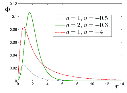
Figure 1: Radial profiles of the modon solution $\Phi(r)$ for different $a$ (cut radius) and $u$ (modon velocity) with $v_{\ast}=1$ and $\alpha=7$.

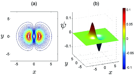
Figure 2: The modon (51) with the parameters $a=2$ (cut radius), $u=-0.3$ (velocity) for $v_{\ast}=1$ and $\alpha=7$. (a) Streamlines $|\psi|$ in the $(x,y)$ plane; (b) modon solution $\psi$.

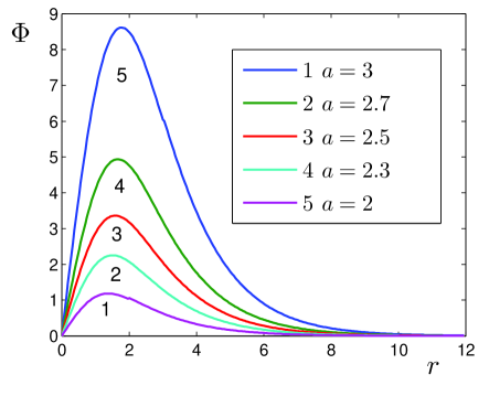
Figure 3: Radial profiles of the modon solution $\Phi(r)$ for different $a$ (cut radius) at the fixed modon velocity $u=-2$ with $v_{\ast}=1$ and $\alpha=2$.

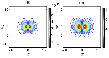
Figure 4: Streamlines $|\psi|$ in the $(x,y)$ plane at the fixed modon velocity $u=-2$ and different $a$ with $v_{\ast}=1$ and $\alpha=2$. a) $a=1$; b) $a=3$.

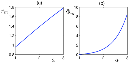
Figure 5: (a) Dependence of the radial position of the maximum of the radial part (amplitude) of the modon $r_{m}$ on the separatrix radius $a$; (b) dependence of the amplitude of the radial part of the modon $\Phi_{m}$ on the separatrix radius $a$; the parameters: $u=-2$, $v_{\ast}=1$ and $\alpha=2$.

The coefficients $A$, $B$, $C$, and $D$ in Eqs. (26) and (30) are given by Eq. (49), and the constant $c_{2}$ is determined from Eq. (50). Note that the transcendental equation (50) has an infinite set of roots $c_{2,n}$, $n=1,2\dots$ for each fixed pair of values of the free parameters $u$ (velocity) and $a$ (separatrix radius). The solution with $n=1$ (the ground-state modon) has no radial nodes. Further, we consider only the ground-state modon with $c_{2,1}\equiv c_{2}$. Equation (50) for $c_{2}$ can be readily solved, and then the coefficients $A$, $B$, $C$, and $D$ are uniquely determined, and with them the exact solution (51) is found that is continuous on the separatrix $r=a$ up to the fourth derivative. Radial profiles of the modon solution $\Phi(r)$ for different $a$ (cut radius) and $u$ (modon velocity) are plotted in Fig. 1. In all these cases shown, we fix the parameters $v_{\ast}=1$ and $\alpha=7$. Note that the point $r_{m}$ corresponding to the maximum of the function $\Phi(r)$ is always located to the left of the cut radius point, $r_{m}<a$ ($\Phi(r)$ has an extremum only in the internal region). Streamlines $|\psi|$ in the $(x,y)$ plane and the modon solution (51) are shown in Fig. 2. We also plotted in Fig. 3 the radial parts of the modon solution for several values of the separatrix radius $a$ at a fixed modon velocity $u=-2$ ($v_{\ast}=1$ and $\alpha=2$), and streamlines $|\psi|$ in the $(x,y)$ plane for two different $a$ (Fig. 4). The maximum amplitude of the modon rapidly decreases with decreasing radius of the separatrix $a$, for example, for $a=3$ the maximum amplitude is $\Phi_{m}\approx 8.653$, whereas already for $a=1$ we have $\Phi_{m}\approx 0.062$. The dependence of the position $r_{m}$ of the maximum amplitude (that is, the actual size of the modon) on the radius of the separtrix turns out to be almost linear. The dependences of $r_{m}$ and maximum amplitude of the modon $\Phi_{m}$ on the radius of the separatrix $a$ at a fixed $u=-2$ are presented in Fig. 5.

In the limit $u\rightarrow 0$ with $a$ fixed from Eq. (18) one can see that the solution in the outer region must be equal to zero. In Eqs. (44)-(48) we then have $A$=0 and $B=0$, and to determine $c_{2}$ we find

$$\mu_{1}J_{11}I_{22}=\mu_{2}J_{21}I_{12}.$$ (52)

The coefficients $C$ and $D$ in this case have the form

$$C=\frac{v_{\ast}a\mu_{2}I_{22}}{c_{2}(\mu_{1}J_{21}I_{12}+\mu_{2}J_{11}I_{22})},$$ (53)

$$D=\frac{v_{\ast}a\mu_{1}J_{21}}{c_{2}(\mu_{1}J_{21}I_{12}+\mu_{2}J_{11}I_{22})}.$$ (54)

The solution is

$$\psi(r,\theta)=\begin{cases}\displaystyle\left[CJ_{1}(\mu_{1}r)+DI_{1}(\mu_{2}r)-v_{\ast}r/c_{2}\right]\cos\theta,&r\leqslant a,\\ \displaystyle 0,&r\geqslant a.\end{cases}$$ (55)

Here the nonlinearity acts to completely screen the modon for $r>a$, similar to the modon obtained by Stern Stern1975 . Note that in this case the solution and the first and second derivatives are continuous on the separatrix.

The problem of stability of the found modon is an open and difficult question (as indeed for second-order modons). Here we only note that despite the impressive demonstrations of fully elastic collisions of Larichev-Reznik modons Flierl1980 ; Makino1981 ; Williams1982 and also three-dimensional modons in Lashkin2017 , the question of stability with respect to arbitrary perturbations is still unclear (see, e. g., Swaters2004 and references therein). In particular, in Swaters2004 it was indicated that the Larichev-Reznik modon moving in the negative $x$-direction (in our notation this corresponds to the positive $y$-direction) always undergoes the so-called tilt instability Nycander1992 , which manifests itself under an infinitesimal small perturbation of the direction of modon propagation. Since in our case the found fourth-order modon can only move in the negative $y$-direction, then, at least if we make analogies with the Larichev-Reznik modon, one can expect that the modon we found will not suffer from the tilt instability.

IV Conclusion

We have obtained a two-dimensional nonlinear equation describing the dynamics of disturbances in a rotating self-gravitating fluid under the assumption that the rotation frequency is much higher than the characteristic frequencies of disturbances. The resulting equation contains, in particular, a biharmonic operator in both the linear and nonlinear parts. The nonlinear term is a Poisson bracket (Jacobian). We have obtained a solution in the form of a solitary dipole vortex (modon) using a procedure similar to the Larichev-Reznik method, that is, introducing a cut on a plane (separatrix). The resulting modon solution and all its derivatives up to the fourth order are continuous on the separatrix.

It should be noted that the well-known generalization of the Larichev-Reznik solution Flierl1980 contains, in addition to the dipole part (carrier), also a radially symmetric monopole part (the so-called rider), the amplitude of which is a free parameter and, generally speaking, can significantly exceed the amplitude of the dipole part, although the monopole part does not exist without the dipole one. In this case, the second derivative (and vorticity) has a constant jump on the separatrix. The magnitude of the jump determines the amplitude of the monopole part. In the present paper, we have restricted ourselves to solution (51) without monopole part, although obtaining the corresponding solution with the monopole part can apparently be carried out without difficulty. In this case, however, the fourth derivative of the solution will have a discontinuity.

The found fourth-order modon in the form of a cyclone-anticyclone dipole pair in a self-gravitating fluid can apparently exist in astrophysical objects. For example, the observation of the Mrk 266 galaxy with two nuclei, rotating in the opposite direction was reported in Abrahamyan2020 .

A very interesting task is the numerical simulation of the collision between the found fourth-order modons. We plan to implement this in the future.

AUTHOR DECLARATIONS

Conflict of Interest

The authors have no conflicts to disclose.

Author Contributions

V. M. Lashkin: Conceptualization (equal), Methodology (equal), Validation (equal), Formal analysis (equal), Investigation (equal). O. K. Cheremnykh: Conceptualization (equal), Methodology (equal), Validation (equal), Formal analysis (equal), Investigation (equal).

DATA AVAILABILITY

No data are associated with this manuscript.

V Appendix

This appendix provides the explicit expressions for $\mathcal{A}$, $\mathcal{B}$, $\mathcal{C}$, $\mathcal{D}$, and $G$ in Eq. (49),

$$\mathcal{A}=\lambda_{2}\mu_{1}\mu_{2}\left[\lambda_{2}(\mu_{1}^{2}+\mu_{2}^{2})K_{12}J_{21}I_{22}\right.$$

$$\left.-\mu_{1}(\lambda_{2}^{2}-\mu_{2}^{2})K_{22}J_{11}I_{22}+\mu_{2}(\lambda_{2}^{2}+\mu_{1}^{2})K_{22}J_{21}I_{12}\right],$$ (56)

$$\mathcal{B}=\lambda_{1}\mu_{1}\mu_{2}\left[\mu_{1}(\lambda_{1}^{2}-\mu_{2}^{2})K_{21}J_{11}I_{22}\right.$$

$$\left.-\lambda_{1}(\mu_{1}^{2}+\mu_{2}^{2})K_{11}J_{21}I_{22}-\mu_{2}(\lambda_{1}^{2}+\mu_{1}^{2})K_{21}J_{21}I_{12}\right],$$ (57)

$$\mathcal{C}=\lambda_{1}\lambda_{2}\mu_{2}\left[\lambda_{1}(\lambda_{2}^{2}-\mu_{2}^{2})K_{11}K_{22}I_{22}\right.$$

$$\left.-\lambda_{2}(\lambda_{1}^{2}-\mu_{2}^{2})K_{12}K_{21}I_{22}-\mu_{2}(\lambda_{1}^{2}-\lambda_{2}^{2})K_{21}K_{22}I_{12}\right],$$ (58)

$$\mathcal{D}=\lambda_{1}\lambda_{2}\mu_{1}\left[\lambda_{1}(\lambda_{2}^{2}+\mu_{1}^{2})K_{11}K_{22}J_{21}\right.$$

$$\left.-\lambda_{2}(\lambda_{1}^{2}+\mu_{1}^{2})K_{12}K_{21}J_{21}-\mu_{1}(\lambda_{1}^{2}-\lambda_{2}^{2})K_{21}K_{22}J_{11}\right],$$ (59)

and

$$G=(\lambda_{1}^{2}-\lambda_{2}^{2})(\mu_{1}^{2}+\mu_{2}^{2})\left[\lambda_{1}\lambda_{2}K_{21}K_{22}J_{11}I_{12}\right.$$

$$\left.-\mu_{1}\mu_{2}K_{11}K_{12}J_{21}I_{22}\right]+(\lambda_{1}^{2}+\mu_{1}^{2})(\lambda_{2}^{2}-\mu_{2}^{2})$$

$$\times\left[\lambda_{1}\mu_{1}K_{12}K_{21}J_{21}I_{12}-\lambda_{2}\mu_{2}K_{11}K_{22}J_{11}I_{22}\right]$$

$$+(\lambda_{1}^{2}-\mu_{2}^{2})(\lambda_{2}^{2}+\mu_{1}^{2})\left[\lambda_{1}\mu_{2}K_{12}K_{21}J_{11}I_{22}\right.$$

$$\left.-\lambda_{2}\mu_{1}K_{11}K_{22}J_{21}I_{12}\right].$$ (60)

References

- (1) J. H. Jeans, Astronomy and Cosmogony (Cambridge University Press, Cambridge, 1929).
- (2) A. B. Mikhailovskii, V. I. Petviashvili, and A. M. Fridman, Helical density waves in flat galaxies-moving solitons, JETP Lett. 26, 121 (1977).
- (3) T. Y. Yueh, Nonlinear waves in a self-gravitating medium, Stud. Appl. Math. 65, 1 (1981).
- (4) H. Ono and I. Nakata, Soliton formation in a self-gravitating gas, Progr. of Theor. Phys. 92, 9 (1994).
- (5) T. X. Zhang and X. Q. Li, Nonlinear structures of self-gravitating systems in stable modes, Astron. Astrophys. 294, 339 (1995).
- (6) H. Zhang, X.Q. Li, and Y.H. Ma, -soliton pattern in a self-gravitating fluid disk, Phys. Rev. E 57, 1114 (1998).
- (7) G. Götz, Solitons in Newtonian gravity, Class. Quantum. Grav. 5, 743 (1988).
- (8) F. C. Adams, M. Fatuzzo, and R. Watkins, General analytic results for nonlinear waves and solitons in molecular clouds, Astrophys. J. 426, 629 (1994).
- (9) B. Semelin, N. Sánchez, and H. J. de Vega, Self-gravitating fluid dynamics, instabilities, and solitons, Phys. Rev. D 63, 084005 (2001).
- (10) F. Verheest and P. K. Shukla, Nonlinear waves in multispecies self-gravitating dusty plasmas, Phys. Scr. 55, 83 (1997).
- (11) W. Masood, H. A. Shah, N. L. Tsintsadze, and M. N. S. Qureshi, Dust Alfvén ordinary and cusp solitons and modulational instability in a self-gravitating magneto-radiative plasma, Eur. Phys. J. D 59, 413 (2010).
- (12) T. Cattaert and F. Verheest, Solitary waves in self-gravitating molecular clouds, Astron. Astrophys. 438, 23 (2005).
- (13) V. V. Dolotin and A. M. Fridman, Generation of an observable turbulence spectrum and solitary dipole vortices in rotating gravitating systems, Sov. Phys. JETP 72, 1 (1991).
- (14) D. Jovanović and J. Vranješ, Vortex solitons in self-gravitating plasma, Phys. Scr. 42, 463 (1990).
- (15) P. K. Shukla, Global vortices in nonuniform gravitating systems, Phys. Lett. A 176, 54 (1993).
- (16) N. L. Tsintsadze, J. T. Mendonca, P. K. Shukla, L. Stenflo, and J. Mahmoodi, Regular structures in self-gravitating dusty plasmas, Phys. Scr. 62, 70 (2000).
- (17) O. A. Pokhotelov, V. V. Khruschev, P. K. Shukla, L. Stenflo, and J. F. McKenzie, Nonlinearly coupled Rossby-type and inertio-gravity waves in self-gravitating systems, Phys. Scr. 58, 618 (1998).
- (18) P. K. Shukla and L. Stenflo, Nonlinear vortex chains in a nonuniform gravitating fluid, Astron. Astrophys. 300, 433 (1995).
- (19) M. G. Abrahamyan, Vortices in rotating and gravitating gas disk and in a protoplanetary disk, in Vortex Dynamics Theories and Applications, edited by Z. Harun (IntechOpen, 2020) pp. 1–21.
- (20) V. M. Lashkin, O. K. Cheremnykh, Z. Ehsan, and N. Batool, Three-dimensional vortex dipole solitons in self-gravitating systems, Phys. Rev. E 107, 024201 (2023).
- (21) E. A. Kuznetsov, A. M. Rubenchik, and V. E. Zakharov, Soliton stability in plasmas and hydrodynamics, Phys. Rep. 142, 103-165 (1986).
- (22) E. A. Kuznetsov and V. E. Zakharov, Nonlinear Coherent Phenomena in Continuous Media, in Nonlinear Science at the Dawn of the 21st Century, Lecture Notes in Physics Vol. 542, edited by P. L. Christiansen, M. P. Søerensen, and A. C. Scott (Springer-Verlag, Berlin, 2000), p. 3-46.
- (23) V. E. Zakharov and E. A. Kuznetsov, Solitons and collapses: two evolution scenarios of nonlinear wave systems, Phys.–Usp. 55, 535-556 (2012).
- (24) J. Pedlosky, Geophysical Fluid Dynamics (Springer-Verlag, New York, 1987).
- (25) J. G. Charney, On the scale of atmosperic motions, Geophys. Public. Kosjones Nors. Videnshap.- Akad. Oslo 17, 3 (1948).
- (26) A. Hasegawa and K. Mima, Pseudo-three dimensional turbulence in magnetized nonuniform plasma, Phys. Fluids 21, 87 (1978).
- (27) V. D. Larichev and G. M. Reznik, Strongly nonlinear two-dimensional isolated Rossby waves, Oceanology 16, 547 (1976).
- (28) V. D. Larichev and G. M. Reznik, Two-dimensional Rossby soliton, an exact solution, Rep. U.S.S.R. Acad. Sci. 231, 1077 (1976).
- (29) M. E. Stern, Minimal properties of planetary eddies, J. Mar. Res. 33, 1-13 (1975).
- (30) G. R. Flierl, Isolated eddy models in geophysics, Ann. Rev. Fluid Mech. 19, 493 (1987).
- (31) O. A. Pokhotelov and V. I. Petviashvili, Solitary Waves in Plasmas and in the Atmosphere (Gordon and Breach, Reading, 1992).
- (32) A. I. Berestov, Solitary Rossby waves, Izv. Akad. Nauk SSSR Fiz. Atmos. Okeana 15, 648-654 (1979).
- (33) J. D. Meiss and W. Horton, Solitary drift waves in the presence of magnetic shear, Phys. Fluids 26, 990-997 (1983).
- (34) G. E. Swaters, A perturbation theory for the solitary-drift-vortex solutions of the Hasegawa-Mima equation, J. Plasma Phys. 41, 523-539 (1989).
- (35) M. Ghil, Y. Feliks, L. U. Sushama, Baroclinic and barotropic aspects of the wind-driven ocean circulation, Physica D 167, 1-35 (2002).
- (36) Z. Kizner, G. Reznik, B. Fridman, R. Khvoles, and J. McWilliams, Shallow-water modons on the -plane, J. Fluid Mech. 603, 305-329 (2008).
- (37) N. Lahaue and V. Zeitlin, Coherent magnetic modon solutions in quasi-geostrophic shallow water magnetohydrodynamics, J. Fluid Mech. 941, A15 (2022).
- (38) G. R. Flierl, V. D. Larichev, J. C. McWilliams, and G. M. Reznik, The dynamics of baroclinic and barotropic solitary eddies, Dyn. Atmos. Oceans 5, 1 (1980).
- (39) M. Makino, T. Kamimura, and T. Taniuti, Dynamics of two-dimensional solitary vortices in a low- plasma with convective motion, J. Phys. Soc. Jpn. 50, 980 (1981).
- (40) J. C. McWilliams and N. J. Zabusky, Interactions of isolated vortices I: Modons colliding with modons, Geophys. Astrophys. Fluid. Dyn. 19, 207 (1982).
- (41) V. M. Lashkin, Stable three-dimensional modon soliton in plasmas, Phys. Rev. E 96, 032211 (2017).
- (42) J. Liu and W. Horton, The intrinsic electromagnetic solitary vortices in magnetized plasma, J. Plasma Phys. 36, 1-24 (1986).
- (43) V. P. Lakhin, A. B. Mikhaĭlovskiĭ, and A. I. Smolyakov, Alfven vortices in a plasma with finite ion temperature, Sov. Phys. JETP 65, 898-903 (1987).
- (44) G. D. Aburdzhaniya, Electromagnetic drift vortices in a rotating plasma cylinder, Phys. Scr. 38, 59-63 (1988).
- (45) G. E. Swaters, Spectral properties in modon stability theory, Stud. Appl. Math. 112, 235-258 (2004).
- (46) J. Nycander, Refutation of stability proofs for dipole vortices, Phys. Fluids A 4, 467-476 (1992).