Entanglement Detection by Approximate Entanglement Witnesses
Abstract
The problem of determining whether a given quantum state is separable is known to be computationally difficult. We develop an approach to this problem based on approximations of convex polytopes in high dimensions. By showing that a convex polytope constructed from a polynomial number of hyperplanes approximates the Euclidean ball arbitrarily well in high dimensions, we find evidence that a polynomial-sized set of approximate entanglement witnesses is potentially sufficient to determine the entanglement of a state with high probability.
1 Introduction
The field of quantum computing has seen significant progress since its conceptual inception in the 1950s. The development of algorithms for factoring [18], quantum simulation [13], and solving linear equations [9] are concrete examples where the computational power of quantum computers can potentially surpass that of classical computers. This quantum advantage can be said to emerge from phenomena specific to quantum mechanical systems, in particular superposition and entanglement.
Quantum entanglement is a property of quantum states with multiple subsystems, where the state of the individual subsystems cannot be described without reference to the other systems. Despite its importance, entanglement remains poorly understood; determining whether a given mixed quantum state is separable or entangled is nontrivial even in the simplest bipartite case. For bipartite systems, a solution is known only for (two qubits) and dimensional (qubit and qutrit) systems, and no solution is known for any higher dimensions [6]. In fact, the general problem is NP-hard [5].
One strategy to approach the separability problem is through the use of entanglement witnesses, operators that have positive expectation values on all separable states, and negative expectation values on at least one entangled state. A natural question to ask is how many or what classes of entangled states can a given witness detect, or how many entanglement witnesses are necessary to detect the entanglement of any entangled state? Unfortunately, it was shown that there does not exist a singular or even finite set of entanglement witnesses that can diagnose entanglement in any quantum state with perfect accuracy [19]. In fact, at least an exponential number of entanglement witnesses are necessary to detect even a subset of “robustly” entangled states [16]111There have also been numerical approaches to searching for entanglement witnesses for small numbers of qubits, such as [22]..
In this paper, we will investigate the problem of entanglement detection using a novel method. Motivated by randomized algorithms that obtain greater efficiency by finding approximate solutions 222For example, this occurs when solving semidefinite programming (SDP) problems [1]., we consider modified entanglement witnesses that can sometimes incorrectly detect entanglement in separable states. We want to determine if it is possible to gain efficiency in the number of operators needed to detect entanglement by trading off precision in the sense of allowing a small probability of incorrect classification. Using entanglement witnesses with error may be a useful new method of detecting entanglement if the number of witnesses needed decreases substantially compared to using exact witnesses, while maintaining a success probability that is not too small.
2 Entanglement Witnesses
We introduce some background on quantum entanglement. For a more thorough treatment, see the review by the Horodeckis [8].
2.1 Background
A dimensional quantum pure state is a vector in a dimensional Hilbert space . If we consider a system with composite subsystems, then the total Hilbert space is given by , where is the Hilbert space for each individual subsystem333Note that this assumes factorizability of the Hilbert space, which is guaranteed for qubit systems, though perhaps not for quantum field theories.. Because the operation connecting the spaces is the tensor product, and not the Cartesian product, it is in general not possible to express the overall quantum state as a product of states in each subystem, i.e. 444States that are describable in this form are called product states., where is a state vector corresponding to the state of the -th subsystem. In such a case, we call the state entangled.
In practice, due to the presence of noise and errors, a more general form for a quantum state is needed, which is the quantum mixed state. A quantum mixed state is a positive semi-definite operator operating on a Hilbert space with [14]. We say that a mixed state is separable, a natural generalization of the product state form from above, if it can be written as a convex combination of product states, i.e.
| (1) |
Note that any separable state can be understood as a partial trace over an associated product state. If a mixed state cannot be written in this form, then it is called entangled [6].
Determining whether or not a given mixed state is separable, even in the bipartite case where , is in general quite difficult. Note that this is not the case with pure states, where we can simply find the Schmidt decomposition of the vector (state) in question, and ask if the Schmidt rank is one or not [14]. For mixed states, the separability problem has a solution in the bipartite case only for systems of two qubits or systems of one qubit and one qutrit. The solution, due to the Horodeckis, says that a necessary and sufficient condition for a bipartite state in (two qubits) or dimensions (one qubit and one qutrit) to be separable is if the operator is positive [6]. Here, the operator is the transposition map operating on the second system . This condition is known as the positive partial transpose (PPT) condition [6]. Unfortunately, the PPT criterion is not a sufficient condition for separability of quantum states in dimensions other than the ones stated above. In particular, states that possess bound entanglement, a form of entanglement where no singlets can be distilled with local operations and classical communication (LOCC), are entangled states that violate the positive partial transpose criterion [7].
One fundamental tool in studying mixed state entanglement are entanglement witnesses. Entanglement witnesses are operators that detect entanglement by considering their expectation values on observables [21]. Specifically, an entanglement witness is a Hermitian operator satisfying
| (2) |
for all separable states , and
| (3) |
for at least one entangled state [21]. A crucial property of entanglement witnesses is that for any entangled state, there necessarily exists an entanglement witness that detects its entanglement. This is due to the Hahn-Banach theorem [17], which categorizes an entanglement witness as a separating hyperplane between the convex set of separable states and the entangled state detected by it [21].
Indeed, this geometric interpretation of entanglement witnesses as a separating is not merely superficial; given an entanglement witness , one can construct another witness that detects at least as many entangled states as by a procedure of subtracting positive operators [12]. By iterating this process, one can construct an optimal entanglement witness detecting the maximum number of entangled states possible [12]. Such an entanglement witness is then represented by a hyperplane tangent to the set of separable states.
2.2 Approximate Witnesses
Having discussed the relevant background information on entanglement witnesses, we now introduce the concept of an approximate entanglement witness.
Definition 1.
An approximate entanglement witness is a Hermitian operator acting on a Hilbert space with the following properties:
-
1.
There exists a separable state such that .
-
2.
There exists a separable state such that .
-
3.
There exists an entangled state such that .
The key difference between an approximate entanglement witness and an exact entanglement witness is that there exist separable states where entanglement is incorrectly witnessed for approximate entanglement witnesses. Geometrically, approximate witnesses are represented by secant hyperplanes that intersect the set of separable states, as opposed to exact witnesses that either do not intersect or are tangent to the set of separable states.
The existence of an approximate entanglement witness that detects an entangled state follows directly from the existence of an exact entanglement witness that detects said state. An approximate entanglement witness can be constructed from an exact entanglement witness simply by subtracting positive operators, as in [12].
3 The Set of Separable States
In order for the concept of an approximate entanglement witness to be useful, we need the ability to quantify the accuracy of entanglement detection for a particular approximate witness. Specifically, for a given approximate entanglement witness , we would like to ask how many separable states exist such that . Unfortunately, there is no method that currently exists to determine this quantity. While efforts to study the geometry of the set of separable states have been made, such as in calculating its volume [23, 20] and its inradius [3], the precise shape of this manifold has not yet been ascertained555See [2] for a compilation of results in this field. Hence, we will take an alternative perspective to study this question by transforming the set of separable states to a set that can be studied in greater detail.
4 Spherical Transformation
In this section, we analyze the fraction of separable states that are incorrectly labeled as entangled by considering a toy model of the set of separable states as a unit ball in .
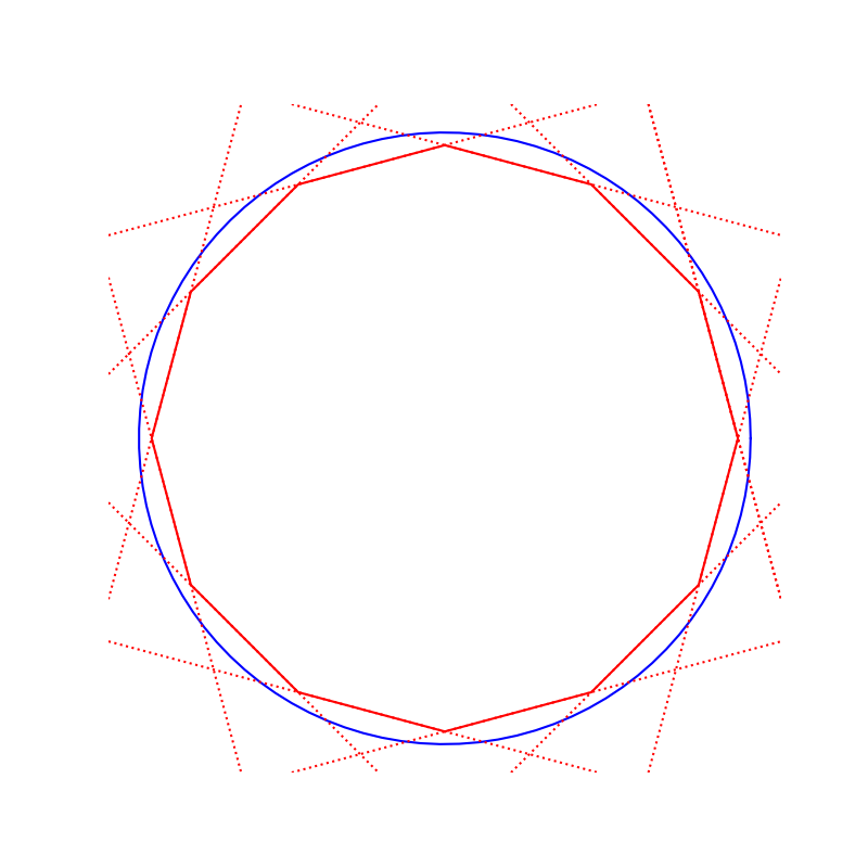
The main result is the statement and proof of Theorem 4.1. Since the set of separable states is a compact convex subset of [10], there exists a homeomorphism that maps it to the closed unit ball . Without finding the explicit transformation, we study the approximate entanglement detection problem by assuming that we have already transformed the set of separable states to a -dimensional ball in Euclidean space, and that an approximate entanglement witness is a hyperplane in that intersects . Under this assumption, we show that when the dimension is large, a polynomially large set of approximate entanglement witnesses is sufficient to approximate the set of separable states666There is also a potential issue with this approach, as it assumes that the homeomorphism between the ball and the set of separable states takes hyperplanes to hyperplanes, something that is not guaranteed. Nevertheless, we believe that finding entanglement witnesses in this toy model is a useful first step to finding complete sets of approximate witnesses for the set of all separable states..
Theorem 4.1.
There exists a polytope with facets that approximates the unit ball so that the ratio between the volume of and the volume of approaches 1 for sufficiently large .
The proof of (4.1) relies on the existence of a polynomial-sized epsilon net for , which was shown in Theorem 1.2 from [15] by Rabani and Shpilka. We restate the result below:
Theorem 4.2.
There exist two universal constants such that for every there is an explicit construction of an -net , for spherical caps of size .
4.1 Proof of Theorem 4.1
Let be fixed. Then by Theorem 4.2, there exists an epsilon net of size . Denote the points in by , for . Consider the hyperplanes defined for each by . Each hyperplane intersects the sphere to form a spherical cap defined by . We construct a polytope contained in using the spherical caps by
| (4) |
A lower bound for the volume of the polytope is then
| (5) |
The volume of a -dimensional ball with radius , denoted by , is known to be
| (6) |
For the unit ball, we have
| (7) |
The volume of the spherical cap can thus be found by integrating the volume of a -dimensional ball with radius from to [11]:
| (8) | ||||
| (9) |
Substituting the expressions for and into , we see that the ratio between the volume of and is bounded below by
| (10) |
Using a small angle approximation for and a Stirling-type approximation for the Gamma functions [4], we can further approximate the volume ratio in (10).
Applying these bounds,
| (12) | ||||
| (13) |
and so
| (14) | ||||
| (15) | ||||
| (16) |
For , we have . Hence,
| (17) |
We see that the volume ratio in equation (10) can be approximated by
| (18) |
Now since , there exists such that for , . It follows that for ,
| (19) |
Since , it’s clear that as , and so for sufficiently large ,
| (20) |
5 Discussion
We have explored the entanglement detection problem through the study of approximate entanglement witnesses. After constructing a toy model of the compact convex set of separable states as a ball , we constructed a convex polytope by removing the spherical caps associated with the intersection of a polynomial number of hyperplanes from the unit ball . We then showed that the difference in volume between the constructed polytope and becomes arbitrarily small as the dimension becomes large.
However, as transforming the set of separable states to a unit ball will not generically cause entanglement witnesses to remain hyperplanes once transformed, since it is in general not true that a hyperplane in one space will remain a hyperplane in a homeomorphic space, we cannot directly apply our result to the set of separable states. Nevertheless, it may be possible to apply our result using alternative methods. For example, one can cover the set of separable states with balls, use our approximation method on each ball, and then construct an approximation to the set of separable states using the polytope approximations for each ball. If the number of balls needed to cover the set is not too large, this would produce an approximation to the set of separable states using not too many approximate entanglement witnesses.
So while we did not find the explicit homeomorphism between the set of separable states and the closed unit ball, our result speaks positively about the potential usefulness of approximate entanglement witnesses. We believe that it is likely that only a polynomial number of approximate witnesses is necessary to detect entangled states with high probability, compared to the super-exponential number of exact entanglement witnesses necessary. In this context, it would be useful to study the geometry of the set of separable states for further investigation.
Acknowledgements
We thank Nathaniel Johnston, Debbie Leung, and Benjamin Lovitz for useful discussions on this topic. N.B. is supported by the Computational Science Initiative at Brookhaven National Laboratory, Northeastern University, and by the U.S. Department of Energy QuantISED Quantum Telescope award.
References
- AHK [05] S. Arora, E. Hazan, and S. Kale. Fast algorithms for approximate semidefinite programming using the multiplicative weights update method. 46th Annual IEEE Symposium on Foundations of Computer Science (FOCS’05), 2005.
- AS [17] Guillaume Aubrun and Stanislaw Szarek. Alice and Bob Meet Banach: The interface of asymptotic geometric analysis and Quantum Information theory. American Mathematical Society, 2017.
- GB [03] Leonid Gurvits and Howard Barnum. Separable balls around the maximally mixed multipartite quantum states. Physical Review A, 68(4), Oct 2003.
- Gor [94] Louis Gordon. A stochastic approach to the gamma function. The American Mathematical Monthly, 101(9):858, 1994.
- Gur [03] Leonid Gurvits. Classical deterministic complexity of edmonds’ problem and quantum entanglement. Proceedings of the thirty-fifth annual ACM symposium on Theory of computing, 2003.
- HHH [96] Michał Horodecki, Paweł Horodecki, and Ryszard Horodecki. Separability of mixed states: Necessary and sufficient conditions. Physics Letters A, 223(1–2):1–8, 1996.
- HHH [98] Michał Horodecki, Paweł Horodecki, and Ryszard Horodecki. Mixed-state entanglement and distillation: Is there a “bound” entanglement in nature? Physical Review Letters, 80(24):5239–5242, Jun 1998.
- HHHH [09] Ryszard Horodecki, Paweł Horodecki, Michał Horodecki, and Karol Horodecki. Quantum entanglement. Reviews of Modern Physics, 81(2):865–942, Jun 2009.
- HHL [09] Aram W. Harrow, Avinatan Hassidim, and Seth Lloyd. Quantum algorithm for linear systems of equations. Physical Review Letters, 103(15), Oct 2009.
- Hor [97] Pawel Horodecki. Separability criterion and inseparable mixed states with positive partial transposition. Physics Letters A, 232(5):333–339, Aug 1997.
- Li [10] S. Li. Concise formulas for the area and volume of a hyperspherical cap. Asian Journal of Mathematics & Statistics, 4(1):66–70, 2010.
- LKCH [00] M. Lewenstein, B. Kraus, J. I. Cirac, and P. Horodecki. Optimization of entanglement witnesses. Physical Review A, 62(5), 2000.
- Llo [96] Seth Lloyd. Universal quantum simulators. Science, 273(5278):1073–1078, Aug 1996.
- NC [10] Michael A. Nielsen and Isaac L. Chuang. Quantum Computation and Quantum Information: 10th Anniversary Edition. Cambridge University Press, 2010.
- RS [22] Yuval Rabani and Amir Shpilka. Corrigendum: Explicit construction of a small epsilon-net for linear threshold functions. SIAM Journal on Computing, 51(5):1692–1702, 2022.
- SA [17] Stanislaw Szarek and Guillaume Aubrun. Dvoretzky’s theorem and the complexity of entanglement detection. Discrete Analysis, page 1–20, 2017.
- SH [99] Helmut H. Schaefer and Wolff Manfred P H. Topological vector spaces. Springer, 1999.
- Sho [97] Peter W. Shor. Polynomial-time algorithms for prime factorization and discrete logarithms on a quantum computer. SIAM Journal on Computing, 26(5):1484–1509, Oct 1997.
- Sko [16] Łukasz Skowronek. There is no direct generalization of positive partial transpose criterion to the three-by-three case. Journal of Mathematical Physics, 57(11), 2016.
- Sza [05] Stanislaw J. Szarek. Volume of separable states is super-doubly-exponentially small in the number of qubits. Physical Review A, 72(3), Sep 2005.
- Ter [00] Barbara M. Terhal. Bell inequalities and the separability criterion. Physics Letters A, 271(5–6):319–326, Jul 2000.
- VBN+ [23] S. V. Vintskevich, N. Bao, A. Nomerotski, P. Stankus, and D. A. Grigoriev. Classification of four-qubit entangled states via machine learning. Physical Review A, 107(3), Mar 2023.
- ŻHSL [98] Karol Życzkowski, Paweł Horodecki, Anna Sanpera, and Maciej Lewenstein. Volume of the set of separable states. Physical Review A, 58(2):883–892, Aug 1998.