Landau Singularities from Whitney Stratifications

Abstract

We demonstrate that the complete and non-redundant set of Landau singularities of Feynman integrals may be explicitly obtained from the Whitney stratification of an algebraic map. As a proof of concept, we leverage recent theoretical and algorithmic advances in their computation, as well as their software implementation, in order to determine this set for several nontrivial examples of two-loop integrals. Interestingly, different strata of the Whitney stratification describe not only the singularities of a given integral, but also those of integrals obtained from kinematic limits, e.g. by setting some of its masses or momenta to zero.

I Introduction

At the heart of both cross-section calculations at the Large Hadron Collider and gravitational wave physics lie the evaluation of Feynman integrals. These integrals are multivalued meromorphic functions of the kinematic variables they depend on, and understanding their analytic structure has been an ongoing quest for theoretical physicists since the late 50’s [1].

Key information on the analytic structure of Feynman integrals is provided by the values of the kinematic variables for which these become singular, this study was initiated in the pioneering work of Landau [2]. A virtue of these Landau singularities, is that knowing them in advance may significantly aid the evaluation of the integrals, for example with the canonical differential equations approach [3]: They may constrain or even fully predict [4] the analytic building blocks or (symbol) letters [5] of this approach, thereby turning the determination of the differential equations from a symbolic, to a much simpler numerical problem. Thanks to their utility, also in other aspects of Feynman integration [6], the analysis of Landau singularities is currently experiencing a revival with ever-increasing momentum, see for example [7, 8, 9, 10, 11, 12, 4, 13, 14].

A mathematically robust definition of what a Landau singularity is has been provided by Pham [15] as his Landau variety; roughly speaking it is characterized by the critical values of a projection map from the variety describing the integrand in terms of all integration and kinematic variables, to the space of just the kinematic variables. Its direct calculation from this definition has proven quite challenging, and much of the recent effort has focused on developing alternative methods that more simply compute varieties that either contain it [7, 8], or are contained in it [4, 13, 14]. In other words, these methods may in general either provide spurious candidates or miss certain Landau singularities entirely, and it is not known when these phenomena do not occur beyond certain special classes of integrals.

In this work, we demonstrate that the rigorous definition of Landau singularities can be used to obtain their complete set, and nothing but their complete set, in a practical manner. To this end, we apply recent theoretical and algorithmic advances on the computation of Whitney stratifications [16, 17], which enter this definition. In particular, we leverage their implementation in the WhitneyStratifications 2.03 package for the Macaulay2 [18] scientific computation software, available at http://martin-helmer.com/Software/WhitStrat/index.html , in order to compute the Landau singularities of several nontrivial two-loop integrals, such as the two-mass hard slashed box and the parachute. While this computational route is currently not as efficient as that of other specialized software for sub- or supersets of Landau singularities [8, 13, 14], it provides a proof of concept that paves the way for their fast and accurate determination in the future.

II Feynman integrals and their singularities

In this article we consider one-particle irreducible Feynman graphs $G:=(E,V)$ with set of edges and vertices $E$ and $V$, respectively, and loop number $L=n-|V|+1$, where we abbreviate $n:=|E|$. The vertex set $V$ has the disjoint partition $V=V_{\mathrm{ext}}\sqcup V_{\mathrm{int}}$ where each vertex $v\in V_{\mathrm{ext}}$ is assigned an external incoming $4$-dimensional momenta $p_{v}\in\mathbb{R}^{1,3}$, and each internal edge $e$ is assigned a mass parameter $m_{e}$. Using dimensional regularization with $D:=4-2\epsilon$ and the Lee-Pomeransky representation [20] we assign the following integral to $G$:

$${}\mathcal{I}=\int_{\mathbb{R}_{+}^{n}}\left(\prod_{i=1}^{n}\frac{x_{i}^{\nu_{i}}\,dx_{i}}{x_{i}\Gamma(\nu_{i})}\right)\,\frac{1}{\mathcal{G}^{D/2}},\qquad\mathcal{G}=\mathcal{U}+\mathcal{F},$$ (1)

where the $\nu_{i}$ are propagator powers and $\mathcal{U}$, respectively $\mathcal{F}$, are the first and second Symanzik polynomials. These are homogeneous polynomials of degree $L$ and $L+1$ in the $x_{i}$, respectively, and may be easily obtained from graph-theoretic data, see e.g. [21]. The polynomial coefficients of $\mathcal{U}$ are just numbers, whereas those of $\mathcal{F}$ depend on the kinematic variables $p_{v},m_{e}$, and are not necessarily algebraically independent.

The study of singularities of Feynman integrals was initially formulated in terms of conditions for their contour of integration to become trapped between colliding poles of the integrand. These conditions are known as the Landau equations [2], which in the representation (1) above read,

$$\mathcal{G}_{h}=0\ \mathrm{and}\ x_{i}\frac{\partial\mathcal{G}_{h}}{\partial x_{i}}=0\ \forall\ i=0,1,\ldots,n,$$ (2)

where $\mathcal{G}_{h}:=\mathcal{U}x_{0}+\mathcal{F}$ is the homogenized Lee-Pomeransky polynomial.

Due to their generically nonlinear nature, directly solving the above equations in an efficient and systematic manner remains a challenge. When the polynomials $\mathcal{U}$ and $\mathcal{F}$ are taken to have generic coefficients, then Landau singularities are alternatively captured by the principal $A$-determinant [22], see also [9]. This is a polynomial in the kinematic variables, which vanishes whenever the equations (2) have a solution.

Despite the algorithmic character of principal $A$-determinant calculations, an issue that arises when specialising the polynomial coefficients back to their Feynman integral values, is that certain factors of the principal $A$-determinant may vanish identically. Given the unphysical conclusion this would lead to, that the Feynman integral is singular for all values of the kinematic variables, one may be tempted to define its Landau singularities by simply removing these vanishing factors. However this definition is incomplete, as it has been definitely shown to miss singularities e.g. in the case of the parachute integral [12]. An empirical refinement of this definition, based on sequential limits of the generic polynomial coefficients, has also been proposed and tested in many one- and some two-loop integrals in [4], yet more extensive vetting and/or a proof would be desirable. Another closely related refinement of the principal $A$-determinant, known as the principal Landau determinant (PLD), has also been recently defined and implemented in the Julia package PLD.jl [13, 14]. Unfortunately, this too appears to miss singularities in certain cases.

A different approach to singularities of integrals is provided by the homological study of integrals depending on parameters. In this setting Pham’s definition of the Landau variety provides a set describing when the topology of $x_{0}\cdots x_{n}\mathcal{G}_{h}=0$ changes. This naturally probes deeper than just considerations of singularities of this variety. An upper bound of the Landau variety is provided by the polynomial reduction described by Brown [7] and is also implemented in HyperInt [8]. A simple sufficient measure for changes in topology is given by the Euler characteristic, which provides a way of reducing this superset closer to the Landau variety. In the case where the Landau variety is equal to the zero set of the principal $A$-determinant it is a corollary of either [23, Theorem 1.1] or [24, Theorem 13] that this superset can be reduced to the Landau variety by only keeping the components where the Euler characteristic of $x_{0}\cdots x_{n}\mathcal{G}_{h}=0$ changes from its generic value. In the general case these results, as well as the result of [25, Corollary 37] relating the number of master integrals to this Euler characteristic, support such an approach to reduce the superset produced by HyperInt to the Landau variety, but we are unaware of any known results which guarantee the correctness of such reductions.

The Landau variety is defined in Section IV, Definition 1, in an algebraic form suitable for direct calculations. In order to do so we require the theory of Whitney stratification, which we introduce in the next section.

III Whitney Stratification Background

Let $k$ be a field, for us this will always be either the real or complex numbers. In the discussion that follows it will be convenient to employ the following notation for the algebraic variety defined by polynomials $g_{1},\dots,g_{r}$ in a polynomial ring $k[x_{1},\dots,x_{n}]$:

$$\mathbf{V}(g_{1},\dots,g_{r}):=\{x\in k^{n}\;|\;g_{1}(x)=\cdots=g_{r}(x)=0\}.$$

Consider an algebraic variety $X$ of dimension $d$. We say a flag $X_{\bullet}$ of varieties $X_{0}\subset\cdots\subset X_{d}=X$ is a Whitney stratification of $X$ if, for all $i$, $X_{i}-X_{i-1}$ is a smooth manifold such that Whitney’s condition B holds for all pairs $M,N$, where $M$ is a connected component of $X_{i}-X_{i-1}$ and $N$ is a connected component of $X_{j}-X_{j-1}$. Such connected components are called strata. A pair of strata, $M,N$ with $\overline{M}\subset\overline{N}$, satisfy Whitney’s condition B at a point $x\in M$ with respect to $N$ if: for every sequence $\{p_{n}\}\subset M$ and every sequence $\{q_{n}\}\subset N$, with $\lim p_{n}=\lim q_{n}=x$, we have $s\subset T$ where $s$ is the limit of secant lines between $p_{n},q_{n}$ and $T$ is the limit of tangent plans to $N$ at $q_{n}$. We say the pair $M,N$ satisfies condition B if condition B holds, with respect to $N$, at all points $x\in M$. This is illustrated in Figures 1 and 2 below.

Note that a Whitney stratification of a variety is not unique, however it was shown in [26, Chapter V–VI] that when $X$ is any complex algebraic (or analytic) variety there exists a unique minimal (or coarsest) Whitney stratification, such that all other Whitney stratifications are obtained by adding strata inside the strata of the minimal one, see also [27, pg. 736–737].

Figure 1: The Whitney stratification of the Whitney cusp, $X=\mathbf{V}(x^{2}+z^{3}-y^{2}z^{2})\subset\mathbb{R}^{3}$, is given by $X\supset\mathbf{V}(x,z)\supset\{(0,0,0)\}$.

Figure 2: Two sequences of points, one on the $y$-axis and one along the top of the surface, both approaching the origin. The limiting secant line is the $z$-axis, while the limiting tangent plane is the $(x,y)$-plane, meaning condition B fails at $(0,0,0)$ for the $y$-axis relative to the rest of the surface. Hence, the origin must be placed in a separate strata from the other points on the $y$-axis.

Consider an algebraic map $f:X\to Y$ between varieties $X$ and $Y$. A Whitney stratification of the map $f$ is a pair $(X_{\bullet},Y_{\bullet})$ where $X_{\bullet}$ is a Whitney stratification of $X$, $Y_{\bullet}$ is a Whitney stratification of $Y$ and for each strata $M$ of $X$ there is a strata $N$ of $Y$ with $f(M)\subset N$ such that the map $f|_{M}:M\to N$ is a submersion, i.e. the differential $df|_{M}$ is surjective. It follows from the existence of the minimal Whitney stratification of a variety and, e.g. the algorithm of [17, §2], that there exists a unique minimal or coarsest stratification of a map as well. Given the defining equations of varieties $X$, $Y$ and of a map $f$ between them, the stratification $(X_{\bullet},Y_{\bullet})$ may be obtained explicitly using the algorithm of [16, 17] as implemented in the WhitneyStratifications Macaulay2 package.

When the map $f$ is proper then we have, by Thom’s First Isotopy Lemma [28, Proposition 11.1], that the topology of the fiber $f^{-1}(q)$ is constant over all points $q\in N$ for any strata $N$ of $Y$.

Example 1 (Topology of Parameterized Cubic)

Consider the planar cubic curve in $\mathbb{R}^{2}$ defined by the parametric polynomial

$$f_{z}(x,y)=(y-1)^{2}-(x-z)x^{2}$$ (3)

in variables $x,y$ with parameter $z$. For parameter values $z<0$ this is a nodal cubic, with one closed loop, while for $z=0$ it is a cusp, and it is a smooth curve with two connected components (over the reals) for positive $z$, see Figure 3. We may use the stratification of the projection map onto the parameter space to detect this change in topology. In particular, if we treat $x,y,z$ as variables, set $X=\mathbf{V}((y-1)^{2}-(x-z)x^{2})\subset\mathbb{R}^{3}$, and consider the projection $\pi:X\to Y=\mathbb{R}$ given by $(x,y,z)\mapsto z$ we may compute a stratification $(X_{\bullet},Y_{\bullet})$ of $\pi$ using methods of [17]. The stratification of $Y=\mathbb{R}$ is given by:

$$\mathbf{V}(z)\subset Y=\mathbb{R}.$$

Hence we see that in particular the topology of the curve changes at $z=0$, dividing $\mathbb{R}-0$ into two connected components, the positive and negative real axis .

This example was used in [14, Example 3.9] to illustrate that the principal Landau determinant, as defined in [14, Definition 3.4 ], fails to capture the change in topology of this curve (and the corresponding change in Euler characteristic); the authors of [14] also give larger examples arising from actual Feynman integrals where the Principal Landau discriminant fails to capture all topological changes which lead to a singular Feynman integral, see [14, §3.5].

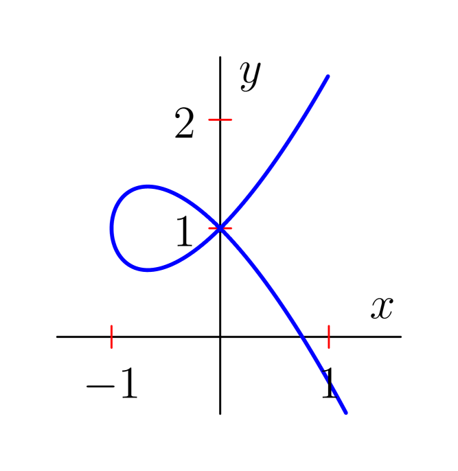
(a) Setting $z=-1$ gives a nodal cubic with one loop.

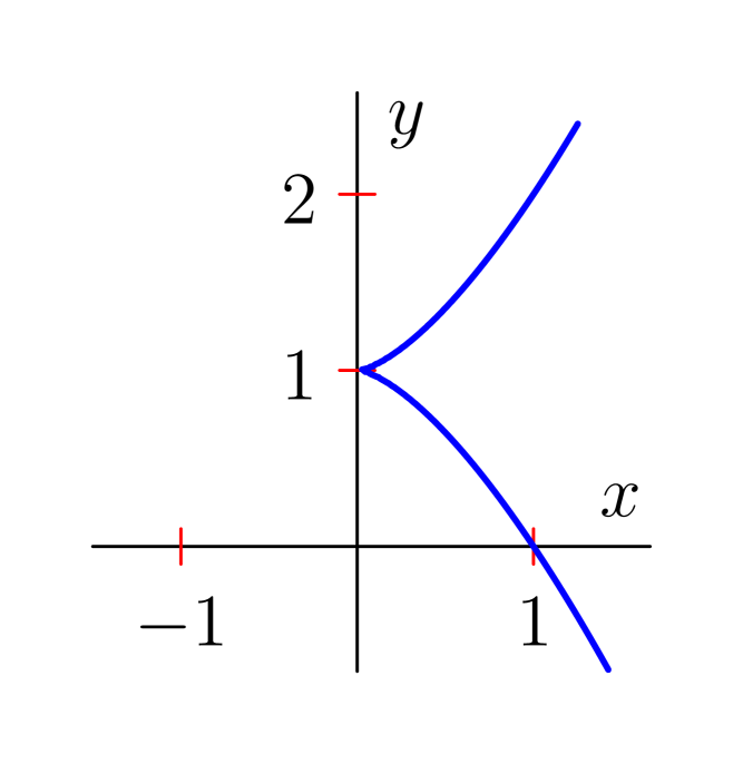
(b) Setting $z=0$ gives a cusp cubic.

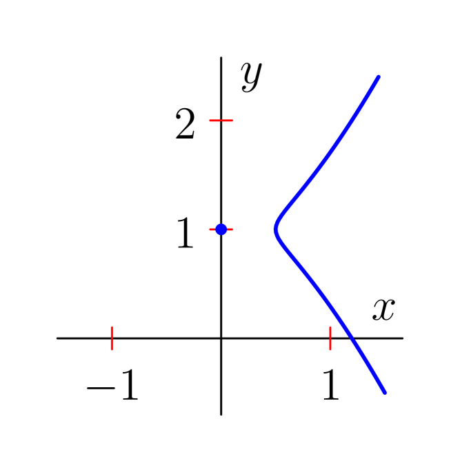
(c) Setting $z=1/2$ gives a curve with two connected components.

Figure 3: Plots of the curve defined by (3) for different parameter values $z$; the topology of the curve changes at $z=0$. While the curve in (3(c)) is smooth and has two connected components (of different dimensions) in $\mathbb{R}^{2}$ it is connected and singular, with singularity at $(0,1)$, in $\mathbb{C}^{2}$.

IV Whitney Stratification of Maps and the Landau Variety

Consider a Feynman integral specified by a polynomial $\mathcal{G}_{h}$ in the ring $\mathbb{C}[z][x]:=\mathbb{C}[z_{1},\dots,z_{m}][x_{0},\dots,x_{n}]$, which is homogeneous in $x$, where the $z_{i}$ are parameters (e.g. masses, momenta) and the $x_{i}$ are variables. For a fixed vector of constants $z$ the resulting polynomial $G_{h}$ is homogeneous and defines a (projective) variety in the complex projective space $\mathbb{P}^{n}$. We make no assumptions on the independence of the parameters, and in particular allow there to be algebraic relations between them. We then seek to describe the Landau variety, which is locus in the parameter space $\mathbb{C}^{m}$ where the Feynman integral is singular; the following definition is (a minor rephrasing of) that of Pham [15, §IV.5] for Feynman integrals in Lee-Pomeransky form:

Definition 1 (Landau variety).

Consider a Feynman integral in Lee-Pomeransky form and let $\mathcal{G}_{h}$ be the $x$-homogeneous polynomial defining it. Set $X=\mathbf{V}(x_{0}\cdots x_{n}\mathcal{G}_{h})\subset\mathbb{P}_{x}^{n}\times\mathbb{C}_{z}^{m}$ and consider the projection map $\pi:X\to\mathbb{C}_{z}^{m}$, then the Landau variety is given by the variety $Y_{m-1}$ appearing in the unique minimal Whitney stratification $(X_{\bullet},Y_{\bullet})$ of the map $\pi$.

Note that the map $\pi$ in Definition 1 is proper by construction, since the fibers are projective varieties (which are always compact), hence Thom’s isotopy lemma always holds for the strata in the map stratification.

Regarding computation, the Whitney stratifications produced by the WhitneyStatifications package have been found to be minimal in all tested cases, however there is currently no theoretical guarantee that this will always be the case. The minimality of a computed stratification may be checked using the results of [27, page 751–752] and standard computational tools, e.g. the SegreClasses Macaulay2 package [30].

It is also interesting to note that the lower dimensional strata in the stratification of $\pi:X\to\mathbb{C}_{z}^{m}$ as in Definition 1 tell us which singular parameter values lead to further topological changes. Hence, in particular, we also obtain the Landau variety for integrals corresponding to kinematic limits which arise from taking parameter values on the original Landau variety, e.g. if we take parameter values in $Y_{m-1}$ which correspond to a kinematic limit, then the Landau variety of this kinematic limit is given by $Y_{m-2}$, and so on.

Hence, more broadly speaking, the stratification in Definition 1 precisely describes all regions of the parameter space such that within each regions any choices of parameters yield a variety $X$ in $\mathbb{P}^{n}$ with constant topology (note we slightly abuse notation here and use $X$ to refer to both the variety in $\mathbb{P}^{n}\times\mathbb{C}^{m}$, where we treat $x,z$ as variables, and the variety in $\mathbb{P}^{n}$ arising from the same equation for a fixed choice of parameter values $z$).

It is shown in [25, Corollary 37] that the number of master integrals is given by the Euler characteristic $|n+1-\chi(\mathbf{V}(x_{0}x_{1}\cdots x_{n}\mathcal{G}_{h}))|$. Since we have that the topology is constant for parameter values outside the Landau variety (this follows from Thom’s Isotopy Lemma since it is the codimension 1 part of of a stratification of the projection map), then the Euler characteristic is constant as well, and hence the number of master integrals is fixed for these parameter choices. Note that in fact our stratification gives us yet more information than this, in particular when combined with the Euler characteristic computation we may identify all possible numbers of master integrals for all choices of parameters, even ones that yield a singularity.

V Example computations

Figure 4: The singularity structure of the one-loop bubble is classical and well-known. We show that the Landau variety not only reproduces these results but that the full Whitney stratification provides the singularities of kinematic limits.

We demonstrate that the Landau variety, Definition 1, can explicitly be calculated and how the result compares to other approaches. Interestingly, often the full Whitney stratification of the map is not needed but it is enough to calculate the stratification of the map imposing only that the successive differences of elements in each of the flags $X_{\bullet},Y_{\bullet}$ are smooth, which can be done by computing consecutive singular loci . The latter is not guaranteed to provide all singularities, but the correctness has been verified a posteriori for the cases considered.

V.1 One-loop bubble

We begin be showing how the full Whitney stratification for the generic one-loop bubble, Figure 4, not only provides the Landau variety but also the singularities in kinematic limits. Let $\mathcal{G}_{h}$ be the homogenized Lee-Pomeransky polynomial for the bubble graph: $\mathcal{G}_{h}=x_{0}(x_{1}+x_{2})+(m_{1}^{2}+m_{2}^{2}-p^{2})x_{1}x_{2}+m_{1}^{2}x_{1}^{2}+m_{2}^{2}x_{2}^{2}$. We have the variety $X=\mathbf{V}(x_{0}x_{1}x_{2}\mathcal{G}_{h})\subset\mathbb{P}^{2}\times\mathbb{C}^{3}$; also let $Y=\mathbb{C}^{3}$ be the space of kinematics. Calculating the (minimal) Whitney stratification $(X_{\bullet},Y_{\bullet})$ of the corresponding projection map $\pi:X\to\mathbb{C}^{3}$ gives the following expression for $Y_{\bullet}$,

$$Y_{3}= Y=\mathbb{C}^{3},$$

$$Y_{2}= \mathbf{V}(m_{1}^{2})\cup\mathbf{V}(m_{2}^{2})\cup\mathbf{V}(p^{2})$$

$$\cup\mathbf{V}(p^{4}+m_{1}^{4}+m_{2}^{4}-2p^{2}m_{1}^{2}-2p^{2}m_{2}^{2}-2m_{1}^{2}m_{2}^{2}),$$

$$Y_{1}= \mathbf{V}(p^{2},\,m_{1}^{2}-m_{2}^{2})\cup\mathbf{V}(m_{2}^{2}-p^{2},\,m_{1}^{2})\cup\mathbf{V}(m_{2}^{2},\,m_{1}^{2}-p^{2})$$

$$\cup\mathbf{V}(p^{2},\,m_{1}^{2})\cup\mathbf{V}(p^{2},\,m_{2}^{2})\cup\mathbf{V}(m_{2}^{2},\,m_{1}^{2}),$$

$$Y_{0}= \mathbf{V}(p^{2},\,m_{1}^{2},\,m_{2}^{2}).$$

Per Definition 1, the components of codimension one, $Y_{2}$, constitutes the Landau variety. As already mentioned, the lower dimensional strata correspond to the Landau variety at certain limits. In the limit $m_{1}\to 0$, the Landau variety is read of from the components in $Y_{1}$ containing a single $m_{1}^{2}$: $\mathbf{V}(m_{2}^{2}-p^{2},\,m_{1}^{2}),\ \mathbf{V}(p^{2},m_{1}^{2})$ and $\mathbf{V}(m_{2}^{2},m_{1}^{2})$. This means that the Landau variety in this limit is $\mathbf{V}(m_{2}^{2}-p^{2})\cup\mathbf{V}(p^{2})\cup\mathbf{V}(m_{2}^{2})$.

In this example this is exactly the same as substituting $m_{1}^{2}=0$ in the original Landau variety, but unlike the stratification the latter is not always guaranteed to work.

We also remark that special kinematic configurations can also be specified in the codomain of the mapStratify command, e.g. the Gram determinant constraint for a six-point process may be specified as the space of kinematics $Y$ and the resulting Whitney stratification will only provide strata satisfying this constraint.

The Landau variety gives information of the full analytic structure of the meromorphic function defined by the integral and not the singularities in the physical region. However, the methods in [17] are capable of calculating Whitney stratifications of real semi-algebraic sets, potentially allowing direct access to the physical singularities as well; we leave this fascinating exploration to a future work.

V.2 Slashed box

Figure 5: The slashed box is one of the simplest graphs where different approaches to calculating Landau singularities do not coincide. This is discussed in Section V.2.

As a first simple two-loop example, we consider the slashed box in Figure 5 with all internal edges massless and the external legs satisfying $p_{1}^{2}=0=p_{3}^{2}$ and $p_{2}^{2}\neq 0,\ p_{4}^{2}\neq 0$. This is a kinematic setup relevant for the two-loop correction of of certain QCD processes [32]. The setup for the calculating the Landau variety is $X=\mathbf{V}(x_{0}\cdots x_{5}\mathcal{G}_{h})\subset\mathbb{P}^{5}\times\mathbb{C}^{4}$, with $Y=\mathbb{C}^{4}$. Calculating the Whitney stratification $(X_{\bullet},Y_{\bullet})$ of the corresponding projection map $\pi:X\to\mathbb{C}^{4}$ gives the following expression for the Landau variety

$$Y_{3}= \mathbf{V}(p_{2}^{2})\cup\mathbf{V}(p_{4}^{2})\cup\mathbf{V}(s)\cup\mathbf{V}(t)$$

$$\cup\mathbf{V}(p_{2}^{2}-s)\cup\mathbf{V}(p_{2}^{2}-t)\cup\mathbf{V}(p_{4}^{2}-s)\cup\mathbf{V}(p_{4}^{2}-t)$$

$$\cup\mathbf{V}(p_{2}^{2}+p_{4}^{2}-s-t)\cup\mathbf{V}(p_{2}^{2}p_{4}^{2}-st)$$

Which is the same as obtained with both HyperInt and the principal Landau determinant.

More interesting is the slashed box with the setup $p_{1}^{2}=0=p_{2}^{2}$ and $p_{3}^{2}\neq 0,\ p_{4}^{2}\neq 0$. The Landau variety now consists of the 9 components

$$Y_{3}= \mathbf{V}(p_{3}^{2})\cup\mathbf{V}(s)\cup\mathbf{V}(st+t^{2}-tp_{3}^{2}-tp_{4}^{2}+p_{3}^{2}p_{4}^{2})$$

$$\cup\mathbf{V}(t-p_{4}^{2})\cup\mathbf{V}(s^{2}-2sp_{3}^{2}+p_{3}^{4}-2sp_{4}^{2}-2p_{3}^{2}p_{4}^{2}+p_{4}^{4})$$

$$\cup\mathbf{V}(t-p_{3}^{2})\cup\mathbf{V}(t)\cup\mathbf{V}(p_{4}^{2})\cup\mathbf{V}(p_{4}^{2}-s-t).$$

which coincide with the result from HyperInt, meanwhile, the principal Landau determinant contains 8 of these components, in particular it is missing $p_{4}^{2}-s-t=0$. That this component is significant can be further strengthened: the Euler characteristic $\chi(\mathbf{V}(x_{0}\cdots x_{5}\mathcal{G}_{h}))$ changes for kinematics on this component and it is a letter in the symbol alphabet for the double box topology studied in [32].

We remark that another way of obtaining all 9 components is the limiting procedure from [4, §3.4] used on the “proper” principal $A$-determinant . That is, using the monomial support for the slashed box but with all coefficients treated as generic and then applying the limit where the coefficients becomes the physical ones.

V.3 Parachute graph

In [12], Berghoff and Panzer showed that the integrand geometry $\{\mathcal{U}=0\}\cup\{\mathcal{F}=0\}\cup\{x_{i}=0,\,i=1,\ldots,4\}$ of the parachute graph (Figure 6) has a special non-normal intersection requiring the sequential blow-up of the projective point $[x_{1}\,:\,x_{2}]$ and $x_{1}+x_{2}=0$ to resolve the geometry. The discriminant of this new hypersurface is (see [12, Eq. (6.15)])

$$p_{3}^{2}(m_{4}^{2}-p_{2}^{2})(m_{3}^{2}-p_{1}^{2})+(m_{3}^{2}-m_{4}^{2}-p_{1}^{2}+p_{2}^{2})(m_{3}^{2}p_{2}^{2}-m_{4}^{2}p_{1}^{2})$$ (4)

which is not captured by either direct principal $A$-determinant calculation nor the principal Landau determinant [14, Eq. (3.18)]. However, it is an output from HyperInt and the Euler characteristic of the hypersurface complement drops from the generic value 19 to the value 18 on it, so it should indeed be a part of the Landau variety. We note that the method of blow-ups to resolve non-transverse intersections is an equivalent alternative method to calculate the Whitney stratification, in the latter cases non-transverse intersections are resolved by imposing the B condition (see Section III).

Figure 6: The full singularity structure of the parachute graph was first uncovered by Berghoff and Panzer in [12]. For restricted kinematics we use Whitney stratifications to find the full Landau variety, including components missed by other methods.

Stratifying the map $\pi:\ \mathbb{P}^{4}\times\mathbb{C}^{7}\to\mathbb{C}^{7}$ is at the current stage of the implementation too taxing. Restricting the kinematics to $\{m_{1}^{2}=1,\,m_{2}^{2}=0,\,m_{3}^{2}=0,\,m_{4}^{2}=2,\,p_{1}^{2}=-1,\,p_{2}^{2}=0\}$ keeping only $p_{3}^{2}$ free, the discriminant (4) reduces to $p_{3}^{2}-1$. Direct integration in HyperInt confirms that this is a letter of the integral . At this reduced kinematic point, calculation of the PLD provides three singularities, $\{p_{3}^{2},\,p_{3}^{2}+2,\,p_{3}^{2}-2\}$ while the Whitney stratification gives five:

$$Y_{0}=\mathbf{V}(p_{3}^{2})\cup\mathbf{V}(p_{3}^{2}+2)\cup\mathbf{V}(p_{3}^{2}-2)\cup\mathbf{V}(p_{3}^{2}+1)\cup\mathbf{V}(p_{3}^{2}-1).$$

In particular it gives the discriminant (4) at this kinematic point.

VI Conclusions and Outlooks

In this letter we use the Whitney stratification of maps to calculate the Landau variety as defined by Pham. This not only yields the complete set of singularities for the integral at hand but also the singularities for integrals arising as kinematic limits. As the stratification is a taxing computation, the examples in this letter are restricted to two-loop graphs, however, the methods are fully rigorous and in general applicable to any loop order and kinematic set-up. Even more, this method is agnostic to the fact that these are Feynman integrals and can be applied to calculate singularities of any parameterized integral of Euler type, that is, every integral with rational integrand.

In particular, since the Whitney stratification gives the full Landau variety, we are able to calculate the singularities that the naive principal $A$-determinant or the principal Landau determinant misses.

That discriminant based methods miss certain singularities provokes the obvious question: is anything special about these singularities, both from a physical and mathematical perspective? In forthcoming work we will expand on this by strengthen the connection between stratified maps, blow-ups and Euler characteristics.

Finally we note that the current implementation of the map stratification algorithms is general purpose, being applicable to any algebraic map between any two varieties, and does not take any special advantage of the highly structured nature of the input in the Feynman integral context. Hence, there is hope for substantial performance improvements if more specialized implementations are developed.