Spatio-Temporal Dynamics of Nucleo-Cytoplasmic Transport

Abstract

Nucleocytoplasmic transport is essential for cellular function, presenting a canonical example of rapid molecular sorting inside cells. It consists of a coordinated interplay between import/export of molecules in/out the cell nucleus. Here, we investigate the role of spatio-temporal dynamics of the nucleocytoplasmic transport and its regulation. We develop a biophysical model that captures the main features of the nucleocytoplasmic transport, in particular, its regulation through the Ran cycle. Our model yields steady-state profiles for the molecular components of the Ran cycle, their relaxation times, as well as the nuclear-to-cytoplasmic molecule ratio. We show that these quantities are affected by their spatial dynamics and heterogeneity within the nucleus. Specifically, we find that the spatial nonuniformity of Ran Guanine Exchange Factor (RanGEF)—particularly its proximity to the nuclear envelope— enhances the Ran cycle’s efficiency. We further show that RanGEF’s accumulation near the nuclear envelope results from its intrinsic dynamics as a nuclear cargo, transported by the Ran cycle itself. Overall, our work highlights the critical role of molecular spatial dynamics in cellular processes, and proposes new avenues for theoretical and experimental inquiries into the nucleocytoplasmic transport.

Eukaryotic cells are organized into functional compartments, such as the nucleus and the cytoplasm. The former houses the genome and DNA-related machinery, the latter contains cytosol and organelles for cellular functions such as protein synthesis and degradation [1]. The boundary between the nucleus and the cytoplasm is delineated by the nuclear envelope (NE) [1], with molecules transported bidirectionally across the NE through nuclear pore complexes (NPCs) [2]. Small molecules, such as ions and nucleotides, can freely diffuse through the NPCs [3, 4, 5], while larger molecules, such as proteins, require a regulated multi-step process [6, 7]. These large cargoes bind to a nuclear transport receptor (NTR), which then transports them in/out of the nucleus, depending if the cargo has a nuclear localization or export signal (NLS/NLS) [7, 8].

While individual molecular translocations through NPCs do not require energy, being thermally driven and facilitated by interactions with nucleoporins inside the NPC [9, 10, 11, 12], they are part of a complex cycle that is essentially an energy-driven pump [12, 13, 14, 15, 16]. This cycle can generate import/export fluxes against concentration gradients, maintaining the system in a non-equilibrium steady state [16]. This import/export cycle is run by GTP and the asymmetric distribution of a GTPase Ran protein across the NE [17], with RanGDP largely in the cytoplasm and RanGTP in the nucleus [11, 12, 13, 14]. This asymmetry is established by the guanine nucleotide exchange factor (RanGEF) [18, 19, 20, 21], which promotes GDP-to-GTP exchange in the nucleus, as well as the GTPase-activating protein (RanGAP) [22], which in turn facilitates GTP hydrolysis in the cytoplasm. Importantly, RanGEF is bound to chromatin, while RanGAP associates with the cytoplasmic side of NPCs.
The import–export cycles of cargo proteins are tightly regulated by RanGTP. Figure 1 depicts the import cycle, with each cycle using one GTP molecule and resulting in the export of one Ran molecule per cargo . Taken together, the import–export cycles are tightly controlled by the Ran cycle  [16]. Indeed, reversing the RanGTP gradient between the nucleus and cytoplasm leads to an inverted gradient of the cargoes [24].

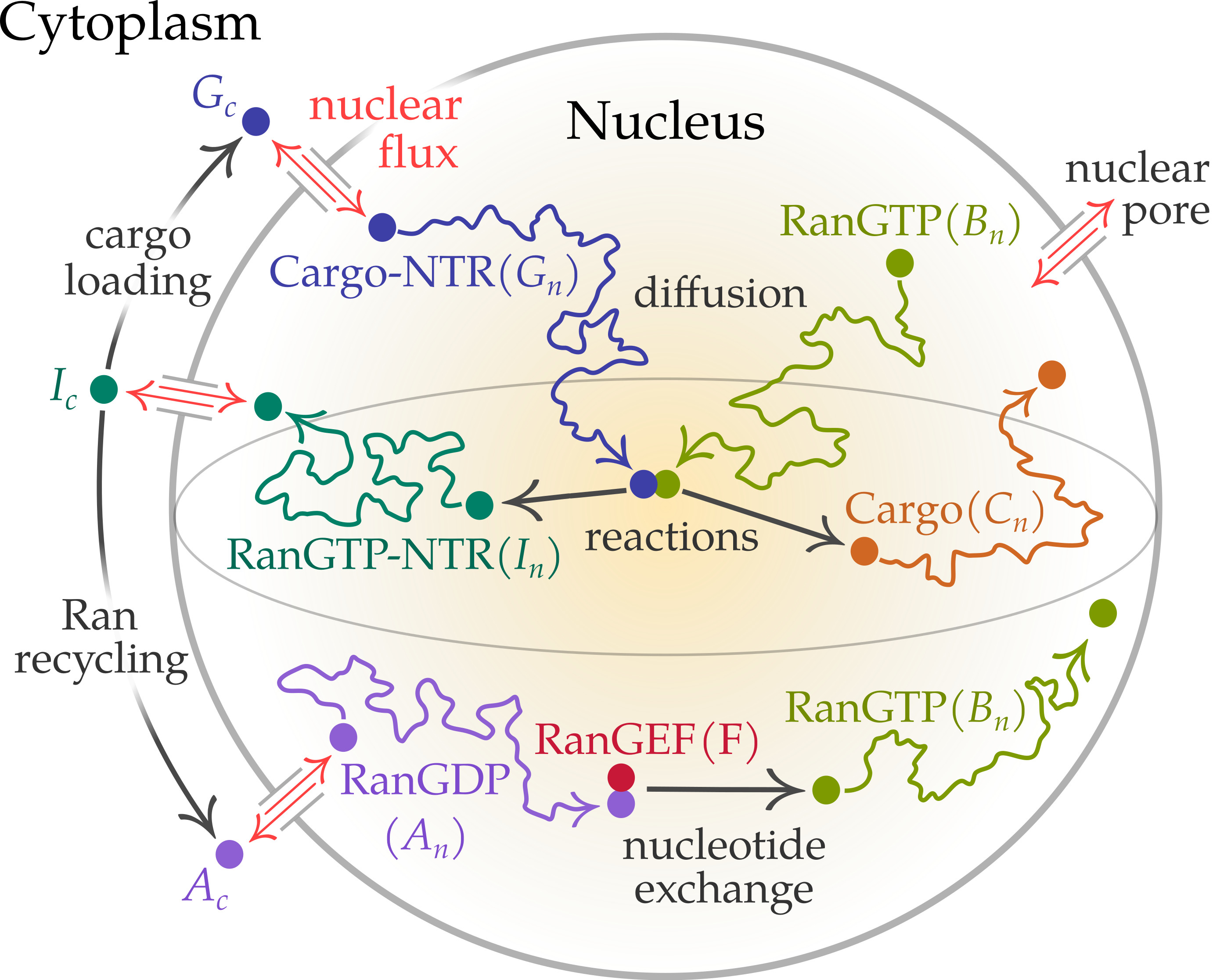
Figure 1: Ran-mediated nuclear transport of a cargo molecule, forming a complex with a nuclear transport receptor (NTR). Cargo-NTR complex passes through nuclear pores, diffuses, and releases the cargo upon RanGTP binding. The RanGTP–NTR complex is recycled to the cytoplasm, where it is dissociated through GTP hydrolysis. RanGDP reenters the nucleus and converts to RanGTP via RanGEF, completing its cycle.

In this study, we investigate the mechanisms behind the nucleo-cytoplasmic transport mediated by the Ran cycle. In contrast to previous studies, which assumed a rapid homogenization of the Ran cycle components within the nucleus and cytoplasm [25, 26, 27, 28, 29, 30, 31, 32, 33, 34, 35, 3, 36], we explore the role of heterogeneity and spatial dynamics of the Ran cycle. To this end, we develop a model of the spatiotemporal transport of Ran components and explore how spatial heterogeneity of RanGEF affects the Ran cycle. We find analytical solutions for steady-state concentrations and relaxation times of Ran components, and obtain ratios of the nuclear to cytoplasmic Ran. We find that localization of RanGEF near the NE significantly increases the Ran content in the nucleus. Lastly, we show that a heterogeneous distribution of RanGEF near the NE originates from its dynamics as a NLS-containing cargo.
Model— We model the nucleus as a sphere of radius $R$ with boundary $\mathcal{S}$ (the NE; $R\simeq 5\,\text{--}\,10\;\mu\mathrm{m}$ [1]) enclosing a volume $\mathcal{V}_{n}$. We assume a constant NPC surface density, providing a uniform flux of particles across the NE [37]. Each NPC supports $10^{2}$–$10^{3}$ translocations per second [36]. The outwards flux at the NE of a molecular species $X$ can be described by $\mathcal{J}_{X}=\lambda_{X}\left(X_{c}-X_{n}\right)$ [25], where $\lambda_{X}$ is the permeability, and the subscripts ${c}$ and ${n}$ denote the cytoplasm and nucleus, respectively. Here, the concentration is the number of molecules per unit volume, ignoring the presence of subnuclear bodies and the polymeric structure of chromatin. The nuclear molecules are assumed to diffuse in the nucleus with an effective constant diffusivity, denoted by $d_{X}$ for a solute $X$, in the range $1-20\,\mu\text{m}^{2}$/s [34, 35]. We do not explicitly account for advection of molecules by nucleoplasmic flows [38, 39, 40, 41, 42, 43, 44, 45, 46], with such an effect, if present, entering only as a contribution to the apparent diffusion constant. We assume that cytoplasmic concentrations are uniform, akin to the experimental conditions of permeabilized cells where the external delivery of molecules is controlled [11]. Thus, at the NE the diffusive flux of molecules is given by

$$-\boldsymbol{n}\cdot d_{X}\boldsymbol{\nabla}X_{n}(\boldsymbol{r},t)+\mathcal{J}_{X}=0,\;\;\boldsymbol{r}\in\mathcal{S},$$ (1)

where $\boldsymbol{n}$ is the outward unit normal to the NE surface $\mathcal{S}$.

We consider the dynamics of the Ran cycle as shown in Fig. 1, where $A$ denotes RanGDP, $B$ is RanGTP, and $I$ is RanGTP–NTR complex. The dynamics of the nuclear RanGDP is given by the reaction–diffusion equation:

$${\partial_{t}A_{n}}=d_{A}\nabla^{2}A_{n}-\alpha(\boldsymbol{r},t)A_{n},\;\;\boldsymbol{r}\in\mathcal{V}_{n},$$ (2)

where $\alpha$ is the nucleotide exchange rate due to RanGEF, converting RanGDP to RanGTP . Similarly, the dynamics of nuclear RanGTP is described by

$${\partial_{t}B_{n}}=d_{B}\nabla^{2}B_{n}+\alpha(\boldsymbol{r},t)A_{n}-\beta(\boldsymbol{r},t)B_{n},\;\;\boldsymbol{r}\in\mathcal{V}_{n},$$ (3)

where $\beta$ is the dissociation rate of cargo molecules from the cargo–NTR complex by binding of RanGTP. We assume $\beta(\boldsymbol{r},t)=b_{0}G_{n}(\boldsymbol{r},t)$, where $b_{0}$ is a constant and $G_{n}$ is the nuclear cargo–NTR concentration given by

$${\partial_{t}G_{n}}=d_{G}\nabla^{2}G_{n}-b_{0}G_{n}B_{n},\;\;\boldsymbol{r}\in\mathcal{V}_{n}.$$ (4)

Also, the cargo dissociation leads to the formation of a nuclear RanGTP–NTR complex ($I_{n}$), which is given by

$${\partial_{t}I_{n}}=d_{I}\nabla^{2}I_{n}+\beta(\boldsymbol{r},t)B_{n},\;\;\boldsymbol{r}\in\mathcal{V}_{n}.$$ (5)

The nuclear concentration $C_{n}$ of free cargo follows

$${\partial_{t}C_{n}}=d_{C}\nabla^{2}C_{n}+\beta(\boldsymbol{r},t)B_{n}-\chi(\boldsymbol{r},t)C_{n},\;\,\boldsymbol{r}\in\mathcal{V}_{n},$$ (6)

where $\chi$ is the nuclear depletion of cargo, e.g. the transcription factor binding to certain loci on the chromatin.

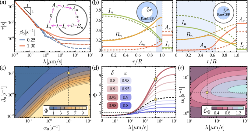
Figure 2: (a) Relaxation time $\tau$ of the Ran cycle (see diagram), when RanGEF is uniform with $\alpha_{0}=5\,\mathrm{s}^{-1}$. Herein, we set the same diffusivity $d=10\,\mu\mathrm{m}^{2}/\mathrm{s}$ for all species, $R=10\,\mu\mathrm{m}$, $\eta=10\,\mathrm{s}^{-1}$, and $\nu={2}/{3}$. Dashed curves are the associated infinite diffusivity limits (same colors). (b) Steady-state concentrations of the Ran-cycle components (as fraction of initial $A_{0}$ concentration). Dashed curves correspond to a uniform RanGEF. In the left plot, solid curves correspond to RanGEF in a shell with inner radius $R\hskip 1.0pt\delta$ (blue region). RanGEF’s net number is the same as in the uniform case, $\alpha_{\mathrm{shell}}=\alpha_{0}/(1-\delta^{3})$. In the right plot, RanGEF is in a ball of radius $R\hskip 1.0pt\varepsilon$ (blue region), with $\varepsilon$ such that $\alpha_{\mathrm{ball}}=\alpha_{0}/\varepsilon^{3}=\alpha_{\mathrm{shell}}$. Here, $\delta=0.9$, $\beta_{0}=1\,\mathrm{s}^{-1}\!$, and $\lambda=10\,\mu\mathrm{m}/\mathrm{s}$. (c) Steady-state $\Phi$ when RanGEF is uniform, with $\lambda=50\,\mu\mathrm{m}/\mathrm{s}$. (d) Steady-state $\Phi$ for the uniform (dashed), shell (purple), and ball (blue) cases, with $\alpha_{0}=10\,\mathrm{s}^{-1}\!$ and $\beta_{0}=1\,\mathrm{s}^{-1}\!$. (e) Relative change $\mathcal{E}_{\Phi}$ of the steady-state $\Phi$ in the shell case compared to $\Phi$ in the uniform case, with $\delta=0.98$. Yellow point and star in (c–e) highlight the same parameter points.

The five reaction–diffusion equations (2–6) are augmented with boundary conditions at the NE, which are given by Eq. (1) with $\mathcal{J}_{A}$, $\mathcal{J}_{G}$, and $\mathcal{J}_{I}$ being nonzero, since their constituents associate with NTRs, while $\mathcal{J}_{B}=\mathcal{J}_{C}=0$, as $B$ and $C$ cannot translocate through NPCs.

In cytoplasm, the homogeneous RanGTP–NTR concentration is described by

$${\partial_{t}I_{c}}=-\eta I_{c}-{\mathcal{V}_{c}^{-1}}\!\textstyle\int_{\mathcal{S}}\hskip 1.0pt{\mathcal{J}_{I}}\,\mathrm{d}S,$$ (7)

where the last term is the exchange of RanGTP–NTR through the NPCs, with $\mathcal{V}_{c}$ as the volume of cytoplasm, whereas the first is the loss due to the GTP hydrolysis by RanGAP, converting RanGTP to RanGDP at a rate $\eta$. Similarly, the cytoplasmic RanGDP is governed by

$${\partial_{t}A_{c}}=\eta I_{c}-{\mathcal{V}_{c}^{-1}}\!\textstyle\int_{\mathcal{S}}\hskip 1.0pt{\mathcal{J}_{A}}\,\mathrm{d}S,\\$$ (8)

while the cytoplasmic cargo–NTR complex follows

$${\partial_{t}G_{c}}=\zeta_{0}N_{c}C_{c}-{\mathcal{V}_{c}^{-1}}\!\textstyle\int_{\mathcal{S}}\hskip 1.0pt{\mathcal{J}_{G}}\,\mathrm{d}S,$$ (9)

where $N_{c}$ is the cytosolic concentration of free NTRs, and $\zeta_{0}$ is the production rate of cargo–NTR complex from a pool of free cargo, with $\partial_{t}C_{c}=-\zeta_{0}N_{c}C_{c}\;+$ other sources or sink terms. NTRs are assumed to be abundant in the cell with $N_{c}$ as a constant. Eqs. (2–9) can be solved by providing initial conditions for each concentration .

Ran cycle under static RanGEF profiles— Since the Ran cycle drives and regulates the nucleocytoplasmic transport, we aim to understand its dynamics and steady-state behavior. We assume that cargo–NTR complexes are in abundance within the cell, so that the cargo dissociation rate $\beta=\beta_{0}$ is treated as a constant. To start, we assume that RanGEF is uniformly distributed with concentration $F_{0}$, where $\alpha=a_{0}F_{0}\equiv\alpha_{0}$ and $a_{0}$ is a constant. Under this approximation, the equations become linear and can be solved by a Laplace transform method [48], choosing an initial condition where Ran is only in the cytoplasm in its GDP-form. The solutions in Laplace space can be used to determine the steady-state concentration profiles and the dominant relaxation time to steady-state [48], as shown in Fig. 2(a) and (b), where, for simplicity, we choose the permeability $\lambda$ and diffusivity $d$ to be the same for all species. Since initially Ran molecules are not present in the nucleus and cytoplasmic concentrations are homogeneous, the solutions to the nuclear concentrations at steady state are found to be radially symmetric, decreasing from the NE into the nucleus with permeation length scales $\ell_{A}=\sqrt{d/\alpha_{0}}$ and $\ell_{B}=\sqrt{d/\beta_{0}}$. These lengths also control the abundance of molecules in the nucleus compared to cytoplasm, where the ratio $\Phi$ of nuclear-to-cytoplasmic Ran molecules is found in exact form [48]. In the physiological regime, $\Phi$ must be greater than unity, around $3$–$4$ [35]. This condition restricts the phase space in terms of local rates, see Fig. 2(c), requiring that $\beta_{0}$ be less than a threshold $\beta_{0}^{\star}$ at which $\Phi=1$, with typically $\beta_{0}^{\star}\simeq 1\,\mathrm{s}^{-1}$. Similarly, this further constrains the permeability $\lambda$, which must be larger than a threshold $\lambda^{\star}$, see Fig. 2(d); typically $\lambda_{\star}\simeq 1\,\mu\mathrm{m}/\mathrm{s}$. Note that if the rates $\alpha_{0}$ and $\beta_{0}$ were known, then knowledge of $\Phi$, which can be measured experimentally [35], allows the estimation of biophysical parameters such as permeability $\lambda$.

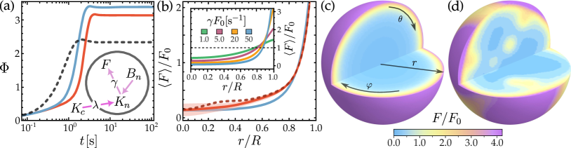
Figure 3: (a) Relaxation of $\Phi$ when RanGEF concentration is uniform (dashed), $\alpha=a_{0}F_{0}=3\,\mathrm{s}^{-1}$. Solid curves are the cases when RanGEF is transported in the nucleus as a complex $K$ (see diagram) and dissociated at a rate $\gamma F_{0}=50\,\mathrm{s}^{-1}$. Initial concentration of $F$ is taken to be: uniform (blue curve), and heterogeneous given by 10 random Gaussian spherical clusters of equal size. Red curve is $\Phi$ averaged over 100 such random initial data. (b) The angular average $\langle F\rangle=\int^{2\pi}_{0}\mathrm{d}\varphi\int^{\pi}_{0}F(r,\theta,\varphi)\sin\theta\mathrm{d}\theta$ of RanGEF at steady-state. Blue and red curves corresponds to the uniform and random initial cases as in (a). Inset shows the dependence on $\gamma$ with RanGEF initially uniform. The blue curve is also depicted in (c). The red shaded region is the standard deviation of the sample around the mean. The red dashed shows one such realization, which is also depicted in figure (d).

Another experimentally measurable quantity [3, 30, 26, 28, 29, 31, 36] is the relaxation time to steady-state of the Ran cycle. In this simple theory, the relaxation time follows from the Laplace space solutions of the concentrations. Specifically, the complex pole $s_{\star}$ with the smallest negative real part in this solution gives us the dominant relaxation time $\tau$; shown in Fig. 2(a). For small values of permeability $\lambda$, we find that $\tau\sim 1/\lambda$, while at larger values of $\lambda$, the system exhibits underdamped oscillations (frequency given by a nonzero imaginary part of $s_{\star}$), where oscillation onset occurs at higher $\lambda$ with increasing $\beta$ [48]. A comparison between $\tau$ and its value in the limit of fast diffusion shows large deviations for $\lambda\gtrsim 1\,\mu\mathrm{m}/\mathrm{s}$, and thus neglecting diffusion may lead to significant errors in the estimation of the relaxation times.
The nucleotide exchange rate depends on the local concentration of RanGEF bound to the chromatin [49], which so far is assumed to be uniformly distributed. However, chromatin density is heterogeneous [50], including heterochromatin. Hence, we investigate next the effect of the RanGEF spatial heterogeneity [51]. For this we study two simple radial distributions of $\alpha(r)$: first, all RanGEF molecules are localized in a spherical shell; and, second, they are all confined to a spherical ball at the center of the nucleus. Assuming piece-wise constant profiles of $\alpha$, the steady-state radial profiles of the concentration fields can be found analytically, and are shown in Fig. 2(b) for the shell and ball cases. In both scenarios, the same total number of RanGEF molecules is chosen as in the entirely uniform case with $\alpha=\alpha_{0}$. The associated steady-states of $\Phi$ are plotted in Fig. 2(d), which shows that distributing RanGEF in a shell near the NE significantly increases the nuclear localization of molecules, when compared to the uniform case; see Fig. 2(e). The increase in $\Phi$ increases with diminishing the shell thickness. Conversely, localizing RanGEF away from the NE (the ball case) has the opposite effect. Thus, a spatial profile for RanGEF can control the nuclear transport.
Dynamics of RanGEF as nuclear cargo— So far we have assumed static RanGEF distributions, however, RanGEF molecules are also NLS-containing cargoes and their nuclear transport is mediated by the Ran cycle [52]. Next, we show that within our model this results in a positive feedback that localizes RanGEF to the nuclear periphery. To begin, we complement the previous equations of the Ran cycle with transport of an additional cargo—receptor complex $K$ that carries RanGEF ($F$); see inset diagram in Fig. 3(a). Using Eqs. (4) and (9), their concentration are described by $\partial_{t}K_{c}=-{\mathcal{V}_{c}^{-1}}\!\int_{\mathcal{S}}\mathcal{J}_{K}\,\mathrm{d}S$ and $\partial_{t}K_{n}=d_{K}\nabla^{2}K_{n}-\gamma B_{n}K_{n}$, satisfying a flux boundary condition as in Eq. (1). The last (nonlinear) term accounts for dissociation of RanGEF cargo at the rate $\gamma B_{n}$. We assume that once free the RanGEF cargo binds rapidly to the chromatin, and its bound concentration is given by $\partial_{t}F=\gamma B_{n}K_{n}$. To complete the model we must set $\alpha=a_{0}F$ and $\beta=\beta_{0}+\gamma K_{n}$.
First, we consider initial distributions $F$ for bound RanGEF which comprise only 10% of the total RanGEF in the cell. The remaining 90% is in the cytoplasm which sets the initial data for $K_{c}$. As before, all Ran molecules are initially in the cytoplasm and in their GDP-form. We solve numerically for the spatial-temporal evolution of the concentration fields [53, 48]. Fig. 3(a) shows the evolution of $\Phi$ for (i) an initially uniform distribution for $F$, and (ii) a distribution $F$ consisting of randomly placed Gaussian spherical clusters of equal standard deviation. The long–time states of $\Phi$ for both (i) and (ii) show an significant increase over the static uniform RanGEF case, as previously computed in Fig. 2(d). Moreover, the long–time concentration profile of chromatin-bound RanGEF shows a sharply varying spatial profile within the nucleus, with a significant accumulation at the NE. To compare the cases (i) and (ii), we compute the angular average of RanGEF, $\langle F\rangle$, which are shown in Fig. 3(b). For case (i), we find at long times a radial profile $\langle F\rangle$ that monotonically decays away from NE with permeation length $\sim\sqrt{d/(\gamma F_{0})}$, which rapidly decreases by increasing the rate $\gamma$; see Fig. 3(b) and (c). For case (ii), the long-time $F$ shows a heterogeneous profile, as shown in the example of Fig. 3(d), where $\langle F\rangle$ also sharply decays away from the NE. By averaging over many such radial profiles $\langle F\rangle$ at long–times, each derived with different initial random data, we determine their mean and standard deviation as shown in Fig. 3(b). This reveals that bound RanGEF displays a significant and sharp accumulation at the NE, despite the initial random distribution.
Discussion— We developed a model exploring the nucleocytoplasmic transport, highlighting the essential role of the spatial distribution and dynamics of the Ran cycle. Our findings demonstrate that the spatial RanGEF distribution directly influences the nucleocytoplasmic transport, in particular, RanGEF’s localization at the NE enhances the Ran cycle efficiency. We find that the sharp accumulation of RanGEF at the NE emerges directly from the transport dynamics of RanGEF molecules as an NLS-containing cargo. Overall, our results suggest that the spatial modulation of the RanGEF substrate may contribute to the regulation of the RanGTP spatial gradient inside cells. With RanGEF having a high affinity for heterochromatin, changes in its organization near the NE could affect the spatial dynamics of RanGEF, and thus in turn the nucleocytoplasmic transport. Understanding how changes in heterochromatin influence RanGEF localization may offer insights into cell’s progression through the cell cycle as well as diseases, where nucleus-wide chromatin organization is disrupted. Our results open new avenues for further theoretical and experimental inquiries into the role of spatial dynamics of molecules in the nucleocytoplasmic transport.

The authors gratefully acknowledge funding from National Science Foundation Grants No. CMMI-1762506 and No. DMS-2153432 (A. Z. and M. J. S.), No. CAREER PHY-1554880 and No. PHY-2210541 (A. Z.). The authors aslo thank D. Saintillan, J. Alsous, A. Lamson, S. Weady, and B. Chakrabarti for illuminating discussions and helpful feedback.

References

- Alberts et al. [2008] B. Alberts, A. Johnson, J. Lewis, M. Raff, K. Roberts, and P. Walter, Molecular Biology of the Cell, 5th ed. (Garland Science, 2008).
- Wente and Rout [2010] S. R. Wente and M. P. Rout, Cold Spring Harbor Perspectives in Biology 2, a000562 (2010).
- Timney et al. [2016] B. L. Timney, B. Raveh, R. Mironska, J. M. Trivedi, S. J. Kim, D. Russel, S. R. Wente, A. Sali, and M. P. Rout, Journal of Cell Biology 215, 57 (2016).
- Keminer and Peters [1999] O. Keminer and R. Peters, Biophysical Journal 77, 217 (1999).
- Mohr et al. [2009] D. Mohr, S. Frey, T. Fischer, T. Güttler, and D. Görlich, The EMBO Journal 28, 2541 (2009).
- Benarroch [2019] E. E. Benarroch, Neurology 92, 757 (2019).
- Macara [2001] I. G. Macara, Microbiology and Molecular Biology Reviews 65, 570 (2001).
- Cautain et al. [2015] B. Cautain, R. Hill, N. de Pedro, and W. Link, The FEBS Journal 282, 445 (2015).
- Jovanovic-Talisman and Zilman [2017] T. Jovanovic-Talisman and A. Zilman, Biophysical Journal 113, 6 (2017).
- Zheng and Zilman [2023] T. Zheng and A. Zilman, Proceedings of the National Academy of Sciences 120, 10.1073/pnas.2212874120 (2023).
- Yang et al. [2004] W. Yang, J. Gelles, and S. M. Musser, Proceedings of the National Academy of Sciences 101, 12887 (2004).
- Ribbeck et al. [1999] K. Ribbeck, U. Kutay, E. Paraskeva, and D. Görlich, Current Biology 9, 47 (1999).
- Görlich and Kutay [1999] D. Görlich and U. Kutay, Annual Review of Cell and Developmental Biology 15, 607 (1999).
- Cavazza and Vernos [2016] T. Cavazza and I. Vernos, Frontiers in Cell and Developmental Biology 3, 10.3389/fcell.2015.00082 (2016).
- Kubitscheck et al. [2005] U. Kubitscheck, D. Grunwald, A. Hoekstra, D. Rohleder, T. Kues, J. P. Siebrasse, and R. Peters, The Journal of Cell Biology 168, 233 (2005).
- Hoogenboom et al. [2021] B. W. Hoogenboom, L. E. Hough, E. A. Lemke, R. Y. Lim, P. R. Onck, and A. Zilman, Physics Reports 921, 1 (2021).
- Joseph [2006] J. Joseph, Journal of Cell Science 119, 3481 (2006).
- Li et al. [2003] H. Y. Li, D. Wirtz, and Y. Zheng, The Journal of Cell Biology 160, 635 (2003).
- Hutchins et al. [2004] J. R. Hutchins, W. J. Moore, F. E. Hood, J. S. Wilson, P. D. Andrews, J. R. Swedlow, and P. R. Clarke, Current Biology 14, 1099 (2004).
- Cushman et al. [2004] I. Cushman, D. Stenoien, and M. S. Moore, Molecular Biology of the Cell 15, 245 (2004).
- Hitakomate et al. [2010] E. Hitakomate, F. E. Hood, H. S. Sanderson, and P. R. Clarke, BMC Cell Biology 11, 43 (2010).
- Seewald et al. [2002] M. J. Seewald, C. Körner, A. Wittinghofer, and I. R. Vetter, Nature 415, 662 (2002).
- Note [1] For transport proteins like Importin-, which utilize an adaptor protein, Importin-, to attach to the cargo, the energy expenditure involves two molecules of GTP.
- Nachury and Weis [1999] M. V. Nachury and K. Weis, Proceedings of the National Academy of Sciences 96, 9622 (1999).
- Wang et al. [2017] C.-H. Wang, P. Mehta, and M. Elbaum, Physical Review Letters 118, 158101 (2017).
- Görlich et al. [2003] D. Görlich, M. J. Seewald, and K. Ribbeck, The EMBO Journal 22, 1088 (2003).
- Smith [2002] A. E. Smith, Science 295, 488 (2002).
- Kopito and Elbaum [2007] R. B. Kopito and M. Elbaum, Proceedings of the National Academy of Sciences 104, 12743 (2007).
- Kopito and Elbaum [2009] R. B. Kopito and M. Elbaum, HFSP Journal 3, 130 (2009).
- Timney et al. [2006] B. L. Timney, J. Tetenbaum-Novatt, D. S. Agate, R. Williams, W. Zhang, B. T. Chait, and M. P. Rout, The Journal of Cell Biology 175, 579 (2006).
- Riddick and Macara [2007] G. Riddick and I. G. Macara, Molecular Systems Biology 3, 10.1038/msb4100160 (2007).
- Kim and Elbaum [2013a] S. Kim and M. Elbaum, Biophysical Journal 105, 565 (2013a).
- Kim and Elbaum [2013b] S. Kim and M. Elbaum, Biophysical Journal 105, 1997 (2013b).
- Wu et al. [2009] J. Wu, A. H. Corbett, and K. M. Berland, Biophysical Journal 96, 3840 (2009).
- Abu-Arish et al. [2009] A. Abu-Arish, P. Kalab, J. Ng-Kamstra, K. Weis, and C. Fradin, Biophysical Journal 97, 2164 (2009).
- Ribbeck and Görlich [2001] K. Ribbeck and D. Görlich, The EMBO Journal 20, 1320 (2001).
- Winey et al. [1997] M. Winey, D. Yarar, T. H. Giddings, and D. N. Mastronarde, Molecular Biology of the Cell 8, 2119 (1997).
- Ashwin et al. [2019] S. S. Ashwin, T. Nozaki, K. Maeshima, and M. Sasai, Proceedings of the National Academy of Sciences 116, 19939 (2019).
- Miné-Hattab and Chiolo [2020] J. Miné-Hattab and I. Chiolo, Frontiers in Genetics 11, 10.3389/fgene.2020.00800 (2020).
- Oliveira et al. [2021] G. M. Oliveira, A. Oravecz, D. Kobi, M. Maroquenne, K. Bystricky, T. Sexton, and N. Molina, Nature Communications 12, 6184 (2021).
- Oshidari et al. [2020] R. Oshidari, K. Mekhail, and A. Seeber, Trends in Cell Biology 30, 144 (2020).
- Barth et al. [2020] R. Barth, K. Bystricky, and H. A. Shaban, Science Advances 6, 10.1126/sciadv.aaz2196 (2020).
- Zidovska et al. [2013] A. Zidovska, D. A. Weitz, and T. J. Mitchison, Proceedings of the National Academy of Sciences 110, 15555 (2013).
- Saintillan et al. [2018] D. Saintillan, M. J. Shelley, and A. Zidovska, Proceedings of the National Academy of Sciences 115, 11442 (2018).
- Zidovska [2020] A. Zidovska, Current Opinion in Genetics and Development 61, 83 (2020).
- Mahajan et al. [2022] A. Mahajan, W. Yan, A. Zidovska, D. Saintillan, and M. J. Shelley, Physical Review X 12, 041033 (2022).
- Note [2] RanGDP is transported into the nucleus by binding to Nuclear Transport Factor 2 (NTF2). Here we do not explicitly consider the interactions with NTF2. We assume that the rate of nucleotide exchange for Ran is not limited by NTF2, assuming the RanGDP molecule dissociates rapidly from that complex once it enters the nucleus; though its dissociation mechanism still remains elusive.
- Note [3] See Supplemental Material.
- Tachibana et al. [2000] T. Tachibana, M. Hieda, Y. Miyamoto, S. Kose, N. Imamoto, and Y. Yoneda, Cell Structure and Function 25, 115 (2000).
- Banerjee et al. [2006] B. Banerjee, D. Bhattacharya, and G. Shivashankar, Biophysical Journal 91, 2297 (2006).
- Dworak et al. [2019] N. Dworak, D. Makosa, M. Chatterjee, K. Jividen, C. Yang, C. Snow, W. C. Simke, I. G. Johnson, J. B. Kelley, and B. M. Paschal, Aging Cell 18, 10.1111/acel.12851 (2019).
- Sankhala et al. [2017] R. S. Sankhala, R. K. Lokareddy, S. Begum, R. A. Pumroy, R. E. Gillilan, and G. Cingolani, Nature Communications 8, 979 (2017).
- Burns et al. [2020] K. J. Burns, G. M. Vasil, J. S. Oishi, D. Lecoanet, and B. P. Brown, Physical Review Research 2, 023068 (2020).