Canonical Decision Diagrams Modulo Theories

Abstract

Decision diagrams (DDs) are powerful tools to represent effectively propositional formulas, which are largely used in many domains, in particular in formal verification and in knowledge compilation. Some forms of DDs (e.g., OBDDs, SDDs) are canonical, that is, (under given conditions on the atom list) they univocally represent equivalence classes of formulas. Given the limited expressiveness of propositional logic, a few attempts to leverage DDs to SMT level have been presented in the literature. Unfortunately, these techniques still suffer from some limitations: most procedures are theory-specific; some produce theory DDs ($\mathcal{T}$-DDs) which do not univocally represent $\mathcal{T}$-valid formulas or $\mathcal{T}$-inconsistent formulas; none of these techniques provably produces theory-canonical $\mathcal{T}$-DDs, which (under given conditions on the $\mathcal{T}$-atom list) univocally represent $\mathcal{T}$-equivalence classes of formulas. Also, these procedures are not easy to implement, and very few implementations are actually available.

In this paper, we present a novel very-general technique to leverage DDs to SMT level, which has several advantages: it is very easy to implement on top of an AllSMT solver and a DD package, which are used as blackboxes; it works for every form of DDs and every theory, or combination thereof, supported by the AllSMT solver; it produces theory-canonical $\mathcal{T}$-DDs if the propositional DD is canonical. We have implemented a prototype tool for both $\mathcal{T}$-OBDDs and $\mathcal{T}$-SDDs on top of OBDD and SDD packages and the MathSAT SMT solver. Some preliminary empirical evaluation supports the effectiveness of the approach.

ignoreinlongenv

1 Introduction

In the field of Knowledge Compilation (KC), the aim is to transform a given knowledge base, often represented as a Boolean formula, into a more suitable form that facilitates efficient query answering. This involves shifting the bulk of computational effort to the offline compilation phase, thereby optimizing the efficiency of the online query-answering phase. Many representations are subsets of Negation Normal Form (NNF), and in particular of decomposable, deterministic NNF (d-DNNF) [18]. Among these, decision diagrams (DDs) such as Ordered Binary Decision Diagrams (OBDDs) [6] and Sentential Decision Diagrams (SDDs) [17] are well-established and widely adopted representations in KC. They offer efficient querying and manipulation of Boolean functions and serve as foundational elements in numerous tools across various domains, including planning [27], probabilistic inference [5, 35], probabilistic reasoning [12, 21], and formal verification [8]. Central to KC is the notion of canonicity, where two equivalent Boolean formulas yield identical decision diagrams. Under specific conditions, both OBDDs and SDDs can achieve canonicity.

The literature on KC, decision diagrams, and canonicity for Boolean formulas is extensive. However, there is a notable scarcity of literature addressing scenarios where formulas contain first-order logic theories such as difference logic ($\mathcal{DL}$), two variables per inequality ($\mathcal{TVPI}$), linear and non-linear arithmetic ($\mathcal{LRA}$ and $\mathcal{NLA}$), and equalities ($\mathcal{E}$) with uninterpreted functions ($\mathcal{EUF}$), which requires leveraging decision diagrams for Satisfiability Modulo Theories (SMT).

Related work.

Most of the literature has focused on theory-aware OBDDs. The majority of the works are theory-specific, in particular focusing on $\mathcal{E}$ [23, 25, 26, 7], $\mathcal{EUF}$ [34, 1, 2], and fragments of arithmetic, such as $\mathcal{DL}$ [30], $\mathcal{TVPI}$ [10], and $\mathcal{NLA}$ [11]. Some general approaches have been proposed to support arbitrary theories [19, 22, 9, 13]. To the best of our knowledge, the only tentative to extend SDDs to support first-order theories are XSDDs [20, 28] which support $\mathcal{LRA}$.

From the practical point of view, most of the techniques are hard to implement since they require modifying the internals of some SMT solver or DD package, or both. Indeed, all of them, with the only exception of LDDs [10], do not have a public implementation, or are implemented within other tools, making them not directly usable and comparable to our approach. From the theoretical point of view, some techniques allow for theory-inconsistent paths (e.g., LDDs [10] and XSDDs [20, 28]), while others only guarantee theory-semicanonicity, i.e., they map all theory-valid and all theory-inconsistent formulas to the same DD (e.g., DDDs [30]). Notably, none of them has been proven to be theory-canonical.

An extensive and detailed analysis of all these techniques is available in the appendix.

Contributions.

In this paper, we investigate the problem of leveraging Boolean decision diagrams (DDs) to SMT level ($\mathcal{T}$-DDs). We present a general formal framework for $\mathcal{T}$-DDs. Then, we introduce a novel and highly versatile technique for extending decision diagrams to the realm of SMT, which operates as follows: we perform a total enumeration of the truth assignments satisfying the input SMT formula (AllSMT) [29], extracting a set of theory lemmas, i.e. $\mathcal{T}$-valid clauses, that rules out all $\mathcal{T}$-inconsistent truth assignments. These $\mathcal{T}$-lemmas are then conjoined to the original SMT problem, and its Boolean abstraction is fed to a Boolean DD compiler to generate a theory DD ($\mathcal{T}$-DD). We formally establish how our proposed framework ensures the generation of $\mathcal{T}$-canonical decision diagrams, provided the underlying Boolean decision diagram is canonical.

Our technique offers several advantages. Firstly, it is very easy to implement, relying on standard AllSMT solvers and existing DD packages as black boxes, with no need to put the hands inside the code of the AllSMT solver and of the DD package. This simplicity makes it accessible to a wide range of users, regardless of their expertise level in SMT solving and DD compiling. Additionally, our technique is theory-agnostic, accommodating any theory or combination thereof supported by the AllSMT solver, and DD-agnostic, since it potentially works with any form of DD. Remarkably, if the underlying DD is canonical, it produces theory-canonical $\mathcal{T}$-DDs, ensuring that two $\mathcal{T}$-equivalent formulas under the same set of theory atoms share the same $\mathcal{T}$-DD. Also, it is the first implementation that can be used for #SMT [31], because the $\mathcal{T}$-DD represents only theory-consistent truth assignments.

We have implemented a prototype of $\mathcal{T}$-OBDD and $\mathcal{T}$-SDD compiler based on our algorithm, using the MathSAT AllSMT solver [16] along with state-of-the-art packages for OBDDs and SDDs. A preliminary empirical evaluation demonstrates the effectiveness of our approach in producing $\mathcal{T}$-canonical $\mathcal{T}$-OBDDs and $\mathcal{T}$-SDDs for several theories.

2 Background

Notation & terminology.

We assume the reader is familiar with the basic syntax, semantics, and results of propositional and first-order logics. We adopt the following terminology and notation.

Satisfiability Modulo Theories (SMT) extends SAT to the context of first-order formulas modulo some background theory $\mathcal{T}$, which provides an intended interpretation for constant, function, and predicate symbols. We restrict to quantifier-free formulas. A $\mathcal{T}$-formula is a combination of theory-specific atoms ($\mathcal{T}$-atoms) via Boolean connectives. For instance, in $\mathcal{LRA}$ $\mathcal{T}$-atoms are linear (in)equalities over rational variables.

${\cal T}2{\cal B}$ is a bijective function (“theory to Boolean”), called Boolean (or propositional) abstraction, which maps Boolean atoms into themselves, $\mathcal{T}$-atoms into fresh Boolean variables, and is homomorphic w.r.t. Boolean operators and set inclusion. The function ${\cal B}2{\cal T}$ (“Boolean to theory”), called refinement, is the inverse of ${\cal T}2{\cal B}$. (For instance ${\cal T}2{\cal B}(\{((x-y\leq 3)\vee(x=z))\})=\{(A_{1}\vee A_{2})\}$, $A_{1}$ and $A_{2}$ being fresh Boolean variables, and ${\cal B}2{\cal T}(\{\neg A_{1},A_{2}\})=\{\neg(x-y\leq 3),(x=z)\}$.)

The symbols ${\boldsymbol{\alpha}}\stackrel{{\scriptstyle\text{\scalebox{0.7}{def}}}}{{=}}\{{\alpha_{i}}\}_{i}$, ${\boldsymbol{\beta}}\stackrel{{\scriptstyle\text{\scalebox{0.7}{def}}}}{{=}}\{{\beta_{i}}\}_{i}$ denote ground $\mathcal{T}$-atoms on $\mathcal{T}$-variables ${\boldsymbol{x}}\stackrel{{\scriptstyle\text{\scalebox{0.7}{def}}}}{{=}}\{{x_{i}}\}_{i}$. The symbols ${\boldsymbol{A}}\stackrel{{\scriptstyle\text{\scalebox{0.7}{def}}}}{{=}}\{{A_{i}}\}_{i}$, ${\boldsymbol{B}}\stackrel{{\scriptstyle\text{\scalebox{0.7}{def}}}}{{=}}\{{B_{i}}\}_{i}$ denote Boolean atoms, and typically denote also the Boolean abstraction of the $\mathcal{T}$-atoms in ${\boldsymbol{\alpha}}$, ${\boldsymbol{\beta}}$ respectively. (Notice that a Boolean atom is also a $\mathcal{T}$-atom, which is mapped into itself by ${\cal T}2{\cal B}$.) We represent truth assignments as conjunctions of literals. We denote by $2^{{\boldsymbol{\alpha}}}$ the set of all total truth assignments on ${\boldsymbol{\alpha}}$. The symbols $\varphi$, $\psi$ denote $\mathcal{T}$-formulas, and $\mu$, $\eta$, $\rho$ denote conjunctions of $\mathcal{T}$-literals; $\varphi^{p}$, $\psi^{p}$ denote Boolean formulas, $\mu^{p}$, $\eta^{p}$, $\rho^{p}$ denote conjunctions of Boolean literals (i.e., truth assignments) and we use them as synonyms for the Boolean abstraction of $\varphi$, $\psi$, $\eta$, and $\rho$ respectively, and vice versa (e.g., $\varphi^{p}$ denotes ${\cal T}2{\cal B}(\varphi)$, $\eta$ denotes ${\cal B}2{\cal T}(\eta^{p})$). If ${\cal T}2{\cal B}(\eta)\models{\cal T}2{\cal B}(\varphi)$, then we say that $\eta$ propositionally (or tautologically) satisfies $\varphi$, written $\eta\models_{\mathbb{B}}\varphi$. (Notice that if $\eta\models_{\mathbb{B}}\varphi$ then $\eta\models_{\mathcal{T}}\varphi$, but not vice versa.) The notion of propositional/tautological entailment and validity follow straightforwardly. When both $\varphi\models_{\mathbb{B}}\psi$ and $\psi\models_{\mathbb{B}}\varphi$, we say that $\varphi$ and $\psi$ are propositionally/tautologically equivalent, written “$\varphi\equiv_{\mathbb{B}}\psi$”. When both $\varphi\models_{\mathcal{T}}\psi$ and $\psi\models_{\mathcal{T}}\varphi$, we say that $\varphi$ and $\psi$ are $\mathcal{T}$-equivalent, written “$\varphi\equiv_{\mathcal{T}}\psi$”. (Notice that if $\eta\equiv_{\mathbb{B}}\varphi$ then $\eta\equiv_{\mathcal{T}}\varphi$, but not vice versa.) We call a $\mathcal{T}$-lemma any $\mathcal{T}$-valid clause.

Decision Diagrams.

Knowledge compilation is the process of transforming a formula into a representation that is more suitable for answering queries [18]. Many known representations are subsets of Negation Normal Form (NNF), which requires formulas to be represented by Directed Acyclic Graphs (DAGs) where internal nodes are labelled with $\land$ or $\lor$, and leaves are labelled with literals $A,\neg A$, or constants $\top,\bot$. Other languages are defined as special cases of NNF [18]. In particular, Decision Diagrams (DDs) like OBDDs and SDDs are popular compilation languages.

Ordered Binary Decision Diagrams (OBDDs) [6] are NNFs where the root node is a decision node and a total order “$<$” on the atoms is imposed. A decision node is either a constant $\top,\bot$, or a $\vee$-node having the form $(A\wedge\varphi)\vee(\neg A\wedge\varphi^{\prime})$, where $A$ is an atom, and $\varphi,\varphi^{\prime}$ are decision nodes. In every path from the root to a leaf, each atom is tested only once, following the order “$<$”. Figure 1 (left) shows a graphical representation of an OBDD, where each decision node is graphically represented as a node labelled with the atom $A$ being tested; a solid and a dashed edge connect it to the nodes of $\varphi$ and $\varphi^{\prime}$, representing the cases in which $A$ is true or false, respectively. OBDDs allow performing many operations in polynomial time, such as performing Boolean combinations of OBDDs, or checking for (un)satisfiability or validity.

SDDs [17] are a generalization of OBDDs, in which decisions are not binary and are made on sentences instead of atoms. Formally, and SDD is an NNF that satisfies the properties of structured decomposability and strong determinism. A v-tree $v$ for atoms ${\boldsymbol{A}}$ is a full binary tree whose leaves are in one-to-one correspondence with the atoms in ${\boldsymbol{A}}$. We denote with $v_{l}$ and $v_{r}$ the left and right subtrees of $v$. A SDD that respects $v$ is either: a constant $\top,\bot$; a literal $A,\neg A$ if $v$ is a leaf labelled with $A$; a decomposition $\bigvee_{i=1}^{n}(\varphi_{i}\wedge\psi_{i})$ if $v$ is internal, $\varphi_{1},...,\varphi_{n}$ are SDDs that respect subtrees of $v_{l}$, $\psi_{1},...,\psi_{n}$ are SDDs that respect subtrees of $v_{r}$, and ${\boldsymbol{\varphi}}\stackrel{{\scriptstyle\text{\scalebox{0.7}{def}}}}{{=}}\{{\varphi_{1},...,\varphi_{n}}\}$ is a partition. ${\boldsymbol{\varphi}}$ is called a partition if each $\varphi_{i}$ is consistent, every pair $\varphi_{i},\varphi_{j}$ for $i\neq j$ are mutually exclusive, and the disjunction of all $\varphi_{i}$s is valid. $\varphi_{i}$s are called primes, and $\psi_{i}$s are called subs. A pair $\varphi_{i},\psi_{i}$ is called an element. Figure 1 (right) shows a graphical representation of a SDD. Decomposition nodes are represented as circles, with an outgoing edge for each element. Elements are represented as paired boxes, where the left and right boxes represent the prime and the sub, respectively. SDDs maintain many of the properties of OBDDs, with the advantage of being exponentially more succinct [4].

These forms of DDs are canonical modulo some canonicity condition $\Lambda$(${\boldsymbol{A}}$) on the Boolean atoms ${\boldsymbol{A}}$: under the assumption that the DDs are built according to the same canonicity condition $\Lambda$(${\boldsymbol{A}}$), then each formula $\varphi^{p}[{\boldsymbol{A}}]$ has a unique DD representation $\textrm{DD}{(\varphi^{p}[{\boldsymbol{A}}])}$, and $\textrm{DD}{(\varphi^{p}[{\boldsymbol{A}}])}=\textrm{DD}{(\varphi^{\prime p}[{\boldsymbol{A}}])}$ if and only if $\varphi^{p}[{\boldsymbol{A}}]\equiv\varphi^{\prime p}[{\boldsymbol{A}}]$ and hence if and only if $\textrm{DD}{(\varphi^{p}[{\boldsymbol{A}}])}\equiv\textrm{DD}{(\varphi^{\prime p}[{\boldsymbol{A}}])}$. (E.g., for OBDDs, $\Lambda$(${\boldsymbol{A}}$) is given total order on ${\boldsymbol{A}}$ [6]; for SDDs $\Lambda$(${\boldsymbol{A}}$) is the structure induced by a given v-tree [17].) Canonicity allows easily checking if a formula is a tautology or a contradiction, and if two formulas are equivalent. Also, canonicity allows storing equivalent subformulas only once.

Figure 1: OBDD (left) and SDD (right) for
$\varphi=(A_{1}\wedge A_{2})\vee(A_{2}\wedge A_{3})\vee(A_{3}\wedge A_{4})$.

3 A Formal Framework for $\mathcal{T}$-DDs

In this section, we introduce the theoretical results that will be used in the rest of the paper. For the sake of compactness, all the proofs of the theorems are deferred to the appendix.

We denote by $\varphi[{\boldsymbol{\alpha}}]$ the fact that ${\boldsymbol{\alpha}}$ is a superset of the set of $\mathcal{T}$-atoms occurring in $\varphi$ whose truth assignments we are interested in. The fact that it is a superset is sometimes necessary for comparing formulas with different sets of $\mathcal{T}$-atoms: $\varphi[{\boldsymbol{\alpha}}]$ and $\varphi^{\prime}[{\boldsymbol{\alpha}}{}^{\prime}]$ can be compared only if they are both considered as formulas on ${\boldsymbol{\alpha}}{}\cup{\boldsymbol{\alpha}}{}^{\prime}$. (E.g., in order to check that $(A_{1}\vee A_{2})\wedge(A_{1}\vee\neg A_{2})$ and $(A_{1}\vee A_{3})\wedge(A_{1}\vee\neg A_{3})$ are equivalent, we need considering them as formulas on $\{{A_{1},A_{2},A_{3}}\}$.)

Given a set of $\mathcal{T}$-atoms ${\boldsymbol{\alpha}}$ and a $\mathcal{T}$-formula $\varphi[{\boldsymbol{\alpha}}]$, we denote by $H_{{\boldsymbol{\alpha}}}(\varphi{})\stackrel{{\scriptstyle\text{\scalebox{0.7}{def}}}}{{=}}\{{\eta_{i}[{\boldsymbol{\alpha}}]}\}_{i}$ and $P_{{\boldsymbol{\alpha}}}(\varphi{})\stackrel{{\scriptstyle\text{\scalebox{0.7}{def}}}}{{=}}\{{\rho_{j}[{\boldsymbol{\alpha}}]}\}_{j}$ respectively the set of all $\mathcal{T}$-consistent and that of all $\mathcal{T}$-inconsistent total truth assignments on the set of $\mathcal{T}$-atoms ${\boldsymbol{\alpha}}{}$ which propositionally satisfy $\varphi$, i.e., s.t.

$$\varphi[{\boldsymbol{\alpha}}]\equiv_{\mathbb{B}}\bigvee_{\eta_{i}[{\boldsymbol{\alpha}}]\in H_{{\boldsymbol{\alpha}}}(\varphi)}\eta_{i}[{\boldsymbol{\alpha}}]\vee\bigvee_{\rho_{j}[{\boldsymbol{\alpha}}]\in P_{{\boldsymbol{\alpha}}}(\varphi)}\rho_{j}[{\boldsymbol{\alpha}}].$$ (1)

The following facts are straightforward consequences of the definition of $H_{{\boldsymbol{\alpha}}}(\varphi{})$ and $P_{{\boldsymbol{\alpha}}}(\varphi{})$.

Proposition 1.

Given two $\mathcal{T}$-formulas $\varphi[{\boldsymbol{\alpha}}]$ and $\varphi^{\prime}[{\boldsymbol{\alpha}}]$, we have that:

• $H_{{\boldsymbol{\alpha}}}(\varphi{})$, $P_{{\boldsymbol{\alpha}}}(\varphi{})$, $H_{{\boldsymbol{\alpha}}}(\neg\varphi{})$, $P_{{\boldsymbol{\alpha}}}(\neg\varphi{})$ are pairwise disjoint;

• $H_{{\boldsymbol{\alpha}}}(\varphi{})\cup P_{{\boldsymbol{\alpha}}}(\varphi{})\cup H_{{\boldsymbol{\alpha}}}(\neg\varphi{})\cup P_{{\boldsymbol{\alpha}}}(\neg\varphi{})=2^{{\boldsymbol{\alpha}}}$;

• $\varphi[{\boldsymbol{\alpha}}]\equiv_{\mathbb{B}}\varphi^{\prime}[{\boldsymbol{\alpha}}]$ if and only if $H_{{\boldsymbol{\alpha}}}(\varphi{})=H_{{\boldsymbol{\alpha}}}(\varphi^{\prime}{})$ and $P_{{\boldsymbol{\alpha}}}(\varphi{})=P_{{\boldsymbol{\alpha}}}(\varphi^{\prime}{})$.

• $\varphi[{\boldsymbol{\alpha}}]\equiv_{\mathcal{T}}\varphi^{\prime}[{\boldsymbol{\alpha}}]$ if and only if $H_{{\boldsymbol{\alpha}}}(\varphi{})=H_{{\boldsymbol{\alpha}}}(\varphi^{\prime}{})$.

Example 2.

Let ${\boldsymbol{\alpha}}{}=\{{\alpha_{1},\alpha_{2}}\}\stackrel{{\scriptstyle\text{\scalebox{0.7}{def}}}}{{=}}\{{(x\leq 0),(x=1)}\}$. Consider the formulas $\varphi_{1}[{\boldsymbol{\alpha}}]\stackrel{{\scriptstyle\text{\scalebox{0.7}{def}}}}{{=}}(x\leq 0)\vee(x=1)$ and $\varphi_{2}[{\boldsymbol{\alpha}}]\stackrel{{\scriptstyle\text{\scalebox{0.7}{def}}}}{{=}}\neg(x\leq 0)\leftrightarrow(x=1)$, so that $\varphi_{1}^{p}[{\boldsymbol{A}}]\stackrel{{\scriptstyle\text{\scalebox{0.7}{def}}}}{{=}}A_{1}\vee A_{2}$ and $\varphi_{2}^{p}[{\boldsymbol{A}}]\stackrel{{\scriptstyle\text{\scalebox{0.7}{def}}}}{{=}}\neg A_{1}\leftrightarrow A_{2}$. It is easy to see that $\varphi_{1}[{\boldsymbol{\alpha}}]\not\equiv_{\mathbb{B}}\varphi_{2}[{\boldsymbol{\alpha}}]$ and $\varphi_{1}[{\boldsymbol{\alpha}}]\equiv_{\mathcal{T}}\varphi_{2}[{\boldsymbol{\alpha}}]$. Then $H_{{\boldsymbol{\alpha}}}(\varphi_{1}[{\boldsymbol{\alpha}}])=H_{{\boldsymbol{\alpha}}}(\varphi_{2}[{\boldsymbol{\alpha}}])=\{{\eta_{1},\eta_{2}}\}=\{{(x\leq 0)\wedge\neg(x=1),\neg(x\leq 0)\wedge(x=1)}\}$, whereas $P_{{\boldsymbol{\alpha}}}(\varphi_{1}[{\boldsymbol{\alpha}}])=\{{(x\leq 0)\wedge(x=1)}\}$ and $P_{{\boldsymbol{\alpha}}}(\varphi_{2}[{\boldsymbol{\alpha}}])=\emptyset$.

3.1 Canonicity for $\text{SMT}(\mathcal{T})$ formulas

Definition 1.

Given a set of $\mathcal{T}$-atoms ${\boldsymbol{\alpha}}$ and its Boolean abstraction ${\boldsymbol{A}}\stackrel{{\scriptstyle\text{\scalebox{0.7}{def}}}}{{=}}{\cal T}2{\cal B}({\boldsymbol{\alpha}}{})$, some $\mathcal{T}$-formula $\varphi[{\boldsymbol{\alpha}}]$, and some form of DDs with canonicity condition $\Lambda$(${\boldsymbol{A}}$) (if any), we call “$\mathcal{T}$-DD$(\varphi[{\boldsymbol{\alpha}}])$” with canonicity condition $\Lambda$(${\boldsymbol{\alpha}}$) an $\text{SMT}(\mathcal{T})$ formula $\Psi[{\boldsymbol{\alpha}}]$ such that $\Psi[{\boldsymbol{\alpha}}]\equiv_{\mathcal{T}}\varphi[{\boldsymbol{\alpha}}]$ and its Boolean abstraction $\Psi^{p}[{\boldsymbol{A}}]$ is a DD.

E.g. “$\mathcal{T}$-OBDDs” and “$\mathcal{T}$-SDDs” denote $\text{SMT}(\mathcal{T})$ extensions of OBDDs and SDDs respectively.

Figure 2: Top: OBDD for $A_{1}\vee A_{2}$ and its refinement for $(x\leq 0)\vee(x=1)$.
Bottom: OBDD for $\neg A_{1}\leftrightarrow A_{2}$ and its refinement for $\neg(x\leq 0)\leftrightarrow(x=1)$.

Theorem 3.

Consider some form of $\mathcal{T}$-DD such that its Boolean abstraction DD is canonical. Then $\textrm{$\mathcal{T}$-DD}{(\varphi[{\boldsymbol{\alpha}}])}=\textrm{$\mathcal{T}$-DD}{(\varphi^{\prime}[{\boldsymbol{\alpha}}])}$ if and only if $\textrm{$\mathcal{T}$-DD}{(\varphi[{\boldsymbol{\alpha}}])}\equiv_{\mathbb{B}}\textrm{$\mathcal{T}$-DD}{(\varphi^{\prime}[{\boldsymbol{\alpha}}])}$.

There are potentially many possible ways by which DDs can be extended into $\mathcal{T}$-DDs, depending mainly on how the $\mathcal{T}$-consistency of branches and subformulas is handled. A straightforward way would be to define it as the refinement of the DD of the Boolean abstraction, i.e. $\textrm{$\mathcal{T}$-DD}{(\varphi[{\boldsymbol{\alpha}}])}\stackrel{{\scriptstyle\text{\scalebox{0.7}{def}}}}{{=}}{\cal B}2{\cal T}(\textrm{DD}{(\varphi^{p}[{\boldsymbol{A}}])})$, without pruning $\mathcal{T}$-inconsistent branches and subformulas. Such $\mathcal{T}$-DDs, however, would be neither $\mathcal{T}$-canonical nor $\mathcal{T}$-semicanonical, as defined below.

Definition 2.

Let ${\boldsymbol{\alpha}}$ be set of $\mathcal{T}$-atoms, and let $\Lambda$(${\boldsymbol{\alpha}}$) be some canonicity condition. We say that a form of $\mathcal{T}$-DD is $\mathbb{B}$-canonical wrt. $\Lambda$(${\boldsymbol{\alpha}}$) iff, for every pair of formulas $\varphi[{\boldsymbol{\alpha}}]$ and $\varphi^{\prime}[{\boldsymbol{\alpha}}]$, $\textrm{$\mathcal{T}$-DD}{(\varphi[{\boldsymbol{\alpha}}])}=\textrm{$\mathcal{T}$-DD}{(\varphi^{\prime}[{\boldsymbol{\alpha}}])}$ if $\varphi[{\boldsymbol{\alpha}}]\equiv_{\mathbb{B}}\varphi^{\prime}[{\boldsymbol{\alpha}}]$.
We say that a form of $\mathcal{T}$-DD is $\mathcal{T}$-canonical wrt. $\Lambda$(${\boldsymbol{\alpha}}$) iff, for every pair of formulas $\varphi[{\boldsymbol{\alpha}}]$ and $\varphi^{\prime}[{\boldsymbol{\alpha}}]$, $\textrm{$\mathcal{T}$-DD}{(\varphi[{\boldsymbol{\alpha}}])}=\textrm{$\mathcal{T}$-DD}{(\varphi^{\prime}[{\boldsymbol{\alpha}}])}$ if and only if $\varphi[{\boldsymbol{\alpha}}]\equiv_{\mathcal{T}}\varphi^{\prime}[{\boldsymbol{\alpha}}]$.
We say that a form of $\mathcal{T}$-DD is $\mathcal{T}$-semicanonical wrt. $\Lambda$(${\boldsymbol{\alpha}}$) iff, for every pair of formulas $\varphi[{\boldsymbol{\alpha}}]$ and $\varphi^{\prime}[{\boldsymbol{\alpha}}]$, if $\varphi[{\boldsymbol{\alpha}}]$ and $\varphi^{\prime}[{\boldsymbol{\alpha}}]$ are both $\mathcal{T}$-inconsistent or are both $\mathcal{T}$-valid, then $\textrm{$\mathcal{T}$-DD}{(\varphi[{\boldsymbol{\alpha}}])}=\textrm{$\mathcal{T}$-DD}{(\varphi^{\prime}[{\boldsymbol{\alpha}}])}$.

If $\mathcal{T}$-DD is $\mathcal{T}$-canonical, then it is also $\mathcal{T}$-semicanonical, but not vice versa. As a consequence of Theorem 3, $\mathcal{T}$-DD is $\mathbb{B}$-canonical if its corresponding DD is canonical, but not vice versa.

Notice the “if” rather than “if and only if” in the definition of $\mathbb{B}$-canonical: it may be the case that $\textrm{$\mathcal{T}$-DD}{(\varphi[{\boldsymbol{\alpha}}])}=\textrm{$\mathcal{T}$-DD}{(\varphi^{\prime}[{\boldsymbol{\alpha}}])}$ even if $\varphi[{\boldsymbol{\alpha}}]\not\equiv_{\mathbb{B}}\varphi^{\prime}[{\boldsymbol{\alpha}}]$ (e.g., if $\varphi[{\boldsymbol{\alpha}}]\equiv_{\mathcal{T}}\varphi^{\prime}[{\boldsymbol{\alpha}}]$, as in the case of $\mathcal{T}$-canonicity).

Example 4.

Let $\mathcal{T}$-OBDD be defined as $\textrm{$\mathcal{T}$-OBDD}{(\varphi_{i}[{\boldsymbol{\alpha}}])}\stackrel{{\scriptstyle\text{\scalebox{0.7}{def}}}}{{=}}{\cal B}2{\cal T}(\textrm{OBDD}{(\varphi_{i}^{p}[{\boldsymbol{A}}])})$. Consider the formulas $\varphi_{1}[{\boldsymbol{\alpha}}],\varphi_{2}[{\boldsymbol{\alpha}}]$ in Example 2. Figure 2 shows the OBDDs for $\varphi_{1}^{p}[{\boldsymbol{A}}]$ and $\varphi_{2}^{p}[{\boldsymbol{A}}]$ (left) –considering as canonicity condition $\Lambda$(${\boldsymbol{A}}$) the order $\{{A_{1},A_{2}}\}$– and the $\mathcal{T}$-OBDDs for $\varphi_{1}[{\boldsymbol{\alpha}}]$ and $\varphi_{2}[{\boldsymbol{\alpha}}]$ (right). Notice that the two $\mathcal{T}$-OBDDs are different despite the fact that $\varphi_{1}[{\boldsymbol{\alpha}}]\equiv_{\mathcal{T}}\varphi_{2}[{\boldsymbol{\alpha}}]$. Thus this form of $\mathcal{T}$-OBDDs is not $\mathcal{T}$-canonical.
Consider the $\mathcal{T}$-valid $\mathcal{T}$-formulas $\varphi_{3}[{\boldsymbol{\alpha}}]\stackrel{{\scriptstyle\text{\scalebox{0.7}{def}}}}{{=}}((x\leq 0)\vee\neg(x\leq 0))\wedge((x=1)\vee\neg(x=1))$ and $\varphi_{4}[{\boldsymbol{\alpha}}]\stackrel{{\scriptstyle\text{\scalebox{0.7}{def}}}}{{=}}\neg(x\leq 0)\vee\neg(x=1)$, so that $\varphi_{3}^{p}[{\boldsymbol{A}}]=(A_{1}\vee\neg A_{1})\wedge(A_{2}\vee\neg A_{2})$ and $\varphi_{4}^{p}[{\boldsymbol{A}}]=\neg A_{1}\vee\neg A_{2}$. Since $\varphi_{3}^{p}[{\boldsymbol{A}}]$ is propositionally valid whereas $\varphi_{4}^{p}[{\boldsymbol{A}}]$ is not, then $\mathcal{T}$-OBDD$(\varphi_{3}[{\boldsymbol{\alpha}}])$ reduces to the $\top$ node whereas $\mathcal{T}$-OBDD$(\varphi_{4}[{\boldsymbol{\alpha}}])$ does not. Dually, $\neg\varphi_{3}[{\boldsymbol{\alpha}}]$ and $\neg\varphi_{4}[{\boldsymbol{\alpha}}]$ are both $\mathcal{T}$-inconsistent, and $\mathcal{T}$-OBDD$(\neg\varphi_{3}[{\boldsymbol{\alpha}}])$ reduces to the $\bot$ node whereas $\mathcal{T}$-OBDD$(\neg\varphi_{4}[{\boldsymbol{\alpha}}])$ does not. Thus this form of $\mathcal{T}$-OBDDs is not $\mathcal{T}$-semicanonical.

Theorem 5.

Consider a form of $\mathcal{T}$-DDs which are $\mathbb{B}$-canonical wrt. some canonicity condition $\Lambda$(${\boldsymbol{\alpha}}$). Suppose that, for every $\text{SMT}(\mathcal{T})$ formula $\varphi[{\boldsymbol{\alpha}}]$, $\textrm{$\mathcal{T}$-DD}{(\varphi[{\boldsymbol{\alpha}}])}\equiv_{\mathbb{B}}\bigvee_{\eta_{i}\in H_{{\boldsymbol{\alpha}}}(\varphi{})}\eta_{i}$. Then $\mathcal{T}$-DD are $\mathcal{T}$-canonical wrt. $\Lambda$(${\boldsymbol{\alpha}}$).

Theorem 5 states a sufficient condition to guarantee the $\mathcal{T}$-canonicity of some form of $\mathcal{T}$-DD: it should represent all and only $\mathcal{T}$-consistent total truth assignments propositionally satisfying the formula. Since typically $\mathcal{T}$-DDs represent partial assignments $\mu_{i}$, the latter ones should not have $\mathcal{T}$-inconsistent total extensions.

3.2 Canonicity via $\mathcal{T}$-lemmas

Definition 3.

We say that a set $\{C_{1}[{\boldsymbol{\alpha}}],\ldots,C_{K}[{\boldsymbol{\alpha}}]\}$ of $\mathcal{T}$-lemmas rules out a set $\{{\rho_{1}[{\boldsymbol{\alpha}}],...,\rho_{M}[{\boldsymbol{\alpha}}]}\}$ of $\mathcal{T}$-inconsistent total truth assignments if and only if, for every $\rho_{j}[{\boldsymbol{\alpha}}]$ in the set, there exists a $C_{l}[{\boldsymbol{\alpha}}]$ s.t. $\rho_{j}[{\boldsymbol{\alpha}}]\models_{\mathbb{B}}\neg C_{l}[{\boldsymbol{\alpha}}]$, that is, if and only if $\bigvee_{j=1}^{M}\rho_{j}[{\boldsymbol{\alpha}}]\wedge\bigwedge_{l=1}^{K}C_{l}[{\boldsymbol{\alpha}}]\equiv_{\mathbb{B}}\bot$.

Given ${\boldsymbol{\alpha}}$ and some $\mathcal{T}$-formula $\varphi[{\boldsymbol{\alpha}}]$, we denote as $Cl_{{\boldsymbol{\alpha}}}(\varphi)$ any function which returns a set of $\mathcal{T}$-lemmas $\{C_{1}[{\boldsymbol{\alpha}}],\ldots,C_{K}[{\boldsymbol{\alpha}}]\}$ which rules out $P_{{\boldsymbol{\alpha}}}(\varphi)$.

Theorem 6.

Let $\varphi[{\boldsymbol{\alpha}}]$ be a $\mathcal{T}$-formula. Let $Cl_{{\boldsymbol{\alpha}}}(\varphi)\stackrel{{\scriptstyle\text{\scalebox{0.7}{def}}}}{{=}}\{C_{1}[{\boldsymbol{\alpha}}],\ldots,C_{K}[{\boldsymbol{\alpha}}]\}{}$ be a set of $\mathcal{T}$-lemmas which rules out $P_{{\boldsymbol{\alpha}}}(\varphi)$. Then we have that:

$$\varphi^{p}[{\boldsymbol{A}}]\ \wedge\bigwedge_{C_{l}[{\boldsymbol{\alpha}}]\in Cl_{{\boldsymbol{\alpha}}}(\varphi)}C_{l}^{p}[{\boldsymbol{A}}]\ \equiv \ \bigvee_{\eta_{i}[{\boldsymbol{\alpha}}]\in H_{{\boldsymbol{\alpha}}}(\varphi{})}\eta_{i}^{p}[{\boldsymbol{A}}].$$ (2)

Theorem 7.

Let ${\boldsymbol{\alpha}}$ denote generical sets of $\mathcal{T}$-atoms with Boolean abstraction ${\boldsymbol{A}}$. Consider some canonical form of DDs on some canonicity condition $\Lambda$(${\boldsymbol{A}}$). Let $\mathcal{T}$-DD with canonicity condition $\Lambda$(${\boldsymbol{\alpha}}$) be such that, for all sets ${\boldsymbol{\alpha}}$ and for all formulas $\varphi[{\boldsymbol{\alpha}}]$:

$$\textrm{$\mathcal{T}$-DD}{}(\varphi[{\boldsymbol{\alpha}}]) \stackrel{{\scriptstyle\text{\scalebox{0.7}{def}}}}{{=}} {\cal B}2{\cal T}{}(\textrm{DD}\left(\varphi^{p}[{\boldsymbol{A}}]\wedge\bigwedge_{C_{l}[{\boldsymbol{\alpha}}]\in Cl_{{\boldsymbol{\alpha}}}(\varphi)}C_{l}^{p}[{\boldsymbol{A}}]\right)).$$ (3)

Then the $\mathcal{T}$-DDs are $\mathcal{T}$-canonical.

Theorem 7 suggests an easy way to implement $\mathcal{T}$-canonical $\mathcal{T}$-DDs by using as $Cl_{{\boldsymbol{\alpha}}}(\varphi)$ the list of $\mathcal{T}$-lemmas produced by an $\text{SMT}(\mathcal{T})$ solver during an AllSMT run over $\varphi[{\boldsymbol{\alpha}}]$. (We will discuss this technique in §4.)

3.3 Dealing with extra $\mathcal{T}$-atoms

Unfortunately, things are not so simple in practice. In order to cope with some theories, AllSMT solvers frequently need introducing extra $\mathcal{T}$-atoms ${\boldsymbol{\beta}}$ on-the-fly, and need generating a set of some extra $\mathcal{T}$-lemmas $\mbox{{\em Defs}}_{{\boldsymbol{\alpha}},{\boldsymbol{\beta}}}(\varphi)\stackrel{{\scriptstyle\text{\scalebox{0.7}{def}}}}{{=}}\{{C_{l}[{\boldsymbol{\alpha}},{\boldsymbol{\beta}}]}\}_{l}$ relating the novel atoms ${\boldsymbol{\beta}}$ with those occurring in the original formula $\varphi[{\boldsymbol{\alpha}}]$ [3]. Consequently, in this case the list of $\mathcal{T}$-lemmas produced by an $\text{SMT}(\mathcal{T})$ solver during an AllSMT run over $\varphi[{\boldsymbol{\alpha}}]$ may contain some of such $\mathcal{T}$-lemmas, and thus they cannot be used as $Cl_{{\boldsymbol{\alpha}}}(\varphi)$.

For instance, when the $\mathcal{LRA}$-atom $(\sum_{i}a_{i}x_{i}=b)$ occurs in a $\mathcal{LRA}$-formula, the SMT solver may need introducing also the $\mathcal{LRA}$-atoms $(\sum_{i}a_{i}x_{i}\geq b)$ and $(\sum_{i}a_{i}x_{i}\leq b)$ and adding some or all the $\mathcal{LRA}$-lemmas encoding $(\sum_{i}a_{i}x_{i}=b)\leftrightarrow((\sum_{i}a_{i}x_{i}\geq b)\wedge(\sum_{i}a_{i}x_{i}\leq b))$.

Definition 4.

We say that a set $\{C_{1}[{\boldsymbol{\alpha}},{\boldsymbol{\beta}}],...,C_{K}[{\boldsymbol{\alpha}},{\boldsymbol{\beta}}]\}$ of $\mathcal{T}$-lemmas on ${\boldsymbol{\alpha}}$,${\boldsymbol{\beta}}$ rules out a set $\{{\rho_{1}[{\boldsymbol{\alpha}}],...,\rho_{M}[{\boldsymbol{\alpha}}]}\}$ of $\mathcal{T}$-inconsistent total truth assignments on ${\boldsymbol{\alpha}}$ if and only if

$$\bigvee_{j=1}^{M}\rho_{j}[{\boldsymbol{\alpha}}]\wedge\bigwedge_{l=1}^{K}C_{l}[{\boldsymbol{\alpha}},{\boldsymbol{\beta}}]\equiv_{\mathbb{B}}\bot.$$ (4)

Given ${\boldsymbol{\alpha}}$, ${\boldsymbol{\beta}}$ and some $\mathcal{T}$-formula $\varphi[{\boldsymbol{\alpha}}]$, we denote as $Cl_{{\boldsymbol{\alpha}},{\boldsymbol{\beta}}}(\varphi)$ any function which returns a set of $\mathcal{T}$-lemmas $\{C_{1}[{\boldsymbol{\alpha}},{\boldsymbol{\beta}}],...,C_{K}[{\boldsymbol{\alpha}},{\boldsymbol{\beta}}]\}$ on ${\boldsymbol{\alpha}}$, ${\boldsymbol{\beta}}$ which rules out $P_{{\boldsymbol{\alpha}}}(\varphi)$. (If ${\boldsymbol{\beta}}=\emptyset$, then Definition 4 reduces to Definition 3 and $Cl_{{\boldsymbol{\alpha}},{\boldsymbol{\beta}}}(\varphi)$ reduces to $Cl_{{\boldsymbol{\alpha}}}(\varphi)$.) Notice that $Cl_{{\boldsymbol{\alpha}},{\boldsymbol{\beta}}}(\varphi)$ is not unique, and it is not necessarily minimal: if $C[{\boldsymbol{\alpha}},{\boldsymbol{\beta}}]\not\in Cl_{{\boldsymbol{\alpha}},{\boldsymbol{\beta}}}(\varphi)$ is a $\mathcal{T}$-lemma, then $\{{C[{\boldsymbol{\alpha}},{\boldsymbol{\beta}}]}\}\cup Cl_{{\boldsymbol{\alpha}},{\boldsymbol{\beta}}}(\varphi)$ rules out $P_{{\boldsymbol{\alpha}}}(\varphi)$ as well. The same fact applies to $Cl_{{\boldsymbol{\alpha}}}(\varphi)$ as well.

Theorem 8.

Let ${\boldsymbol{\alpha}}$ and ${\boldsymbol{\beta}}$ be sets of $\mathcal{T}$-atoms and let ${\boldsymbol{A}}$ and ${\boldsymbol{B}}$ denote their Boolean abstraction. Let $\varphi[{\boldsymbol{\alpha}}]$ be a $\mathcal{T}$-formula. Let $Cl_{{\boldsymbol{\alpha}},{\boldsymbol{\beta}}}(\varphi{})$$\stackrel{{\scriptstyle\text{\scalebox{0.7}{def}}}}{{=}}$ $\{C_{1}[{\boldsymbol{\alpha}},{\boldsymbol{\beta}}],...,C_{K}[{\boldsymbol{\alpha}},{\boldsymbol{\beta}}]\}$ be a set of $\mathcal{T}$-lemmas on ${\boldsymbol{\alpha}}$,${\boldsymbol{\beta}}$ which rules out $P_{{\boldsymbol{\alpha}}}(\varphi)$. Then we have that:

$$\varphi^{p}[{\boldsymbol{A}}]\wedge\exists{\boldsymbol{B}}.\bigwedge_{C_{l}[{\boldsymbol{\alpha}},{\boldsymbol{\beta}}]\in Cl_{{\boldsymbol{\alpha}},{\boldsymbol{\beta}}}(\varphi)}C_{l}^{p}[{\boldsymbol{A}},{\boldsymbol{B}}]\ \equiv \bigvee_{\eta_{i}[{\boldsymbol{\alpha}}]\in H_{{\boldsymbol{\alpha}}}(\varphi)}\eta_{i}^{p}[{\boldsymbol{A}}].$$ (5)

Example 9.

Consider the formula $\varphi_{1}[{\boldsymbol{\alpha}}]\stackrel{{\scriptstyle\text{\scalebox{0.7}{def}}}}{{=}}(x\leq 0)\vee(x=1)$ and its Boolean abstraction $\varphi_{1}^{p}[{\boldsymbol{A}}]\stackrel{{\scriptstyle\text{\scalebox{0.7}{def}}}}{{=}}A_{1}\vee A_{2}$, as in Example 2. If we run an AllSMT solver (e.g. MathSAT) over it we obtain the set $\{{\eta_{1},\eta_{2}}\}\stackrel{{\scriptstyle\text{\scalebox{0.7}{def}}}}{{=}}\{{(x\leq 0)\wedge\neg(x=1),\neg(x\leq 0)\wedge(x=1)}\}$ but, instead of the $\mathcal{T}$-lemma $\neg(x\leq 0)\vee\neg(x=1)$, we might obtain instead five $\mathcal{T}$-lemmas:
$C_{1}:\ \neg(x\leq 0)\vee\neg(x\geq 1)\\ C_{2}:\ \neg(x\leq 0)\vee\phantom{\neg}(x\leq 1)\\ \!C_{3}:\ \neg(x=1)\vee\phantom{\neg}(x\leq 1)\\ \!C_{4}:\ \neg(x=1)\vee\phantom{\neg}(x\geq 1)\\ \!C_{5}:\ \phantom{\neg}(x=1)\vee\neg(x\leq 1)\vee\neg(x\geq 1),$
because the SMT solver has introduced the extra atoms $\{{\beta_{1},\beta_{2}}\}\stackrel{{\scriptstyle\text{\scalebox{0.7}{def}}}}{{=}}\{{(x\leq 1),(x\geq 1)}\}$ and added the axiom $(x=1)\leftrightarrow((x\leq 1)\wedge(x\geq 1))$, which is returned in the list of the $\mathcal{T}$-lemmas as $C_{3},C_{4},C_{5}$.
Now, if we applied the OBDD construction simply to $\varphi^{p}[{\boldsymbol{A}}]\wedge\bigwedge_{i=1}^{5}C_{i}^{p}[{\boldsymbol{A}},{\boldsymbol{B}}]$ and $\varphi[{\boldsymbol{\alpha}}]\wedge\bigwedge_{i=1}^{5}C_{i}[{\boldsymbol{\alpha}},{\boldsymbol{\beta}}]$ respectively, we would obtain the OBDDs in Figure 3, which are much bigger than necessary. Instead, computing the Boolean abstraction and applying the existential quantification on ${\boldsymbol{B}}$ by Shannon’s expansion, we obtain:

$$\varphi^{p}\wedge\exists B_{1}B_{2}.\bigwedge_{l=1}^{5}C_{l}^{p}\ \equiv\ (\overbrace{\phantom{\neg}A_{1}\wedge\neg A_{2}}^{\eta_{1}^{p}[{\boldsymbol{A}}]})\vee(\overbrace{\neg A_{1}\wedge\phantom{\neg}A_{2}}^{\eta_{2}^{p}[{\boldsymbol{A}}]}),$$ (6)

in line with (5) in Theorem 8. The resulting OBDD is that of Figure 2, bottom left.

Figure 3: OBDD for $\varphi^{p}[{\boldsymbol{A}}]\wedge\bigwedge_{i=1}^{5}C^{p}[{\boldsymbol{A}},{\boldsymbol{B}}]$ and its refinement for $\varphi[{\boldsymbol{\alpha}}]\wedge\bigwedge_{i=1}^{5}C[{\boldsymbol{\alpha}},{\boldsymbol{\beta}}]$.

Theorem 10.

Let ${\boldsymbol{\alpha}}$, ${\boldsymbol{\beta}}$ and ${\boldsymbol{\beta^{\prime}}}$ be sets of $\mathcal{T}$-atoms and let ${\boldsymbol{A}}$, ${\boldsymbol{B}}$ and ${\boldsymbol{B^{\prime}}{}}$ denote their Boolean abstraction. Let $\varphi[{\boldsymbol{\alpha}}]$ and $\varphi^{\prime}[{\boldsymbol{\alpha}}]$ be $\mathcal{T}$-formulas. Let $Cl_{{\boldsymbol{\alpha}},{\boldsymbol{\beta}}}(\varphi{})$ be a set of $\mathcal{T}$-lemmas on ${\boldsymbol{\alpha}}$,${\boldsymbol{\beta}}$ which rules out $P_{{\boldsymbol{\alpha}}}(\varphi)$ and $Cl_{{\boldsymbol{\alpha}},{\boldsymbol{\beta^{\prime}}}}(\varphi^{\prime}{})$ be a set of $\mathcal{T}$-lemmas on ${\boldsymbol{\alpha}}$,${\boldsymbol{\beta^{\prime}}}$ which rules out $P_{{\boldsymbol{\alpha}}}(\varphi^{\prime})$. Then $\varphi[{\boldsymbol{\alpha}}]\equiv_{\mathcal{T}}\varphi^{\prime}[{\boldsymbol{\alpha}}]$ if and only if

$$\varphi^{p}[{\boldsymbol{A}}]\wedge\exists{\boldsymbol{B}}.\bigwedge_{C_{l}[{\boldsymbol{\alpha}},{\boldsymbol{\beta}}]\in Cl_{{\boldsymbol{\alpha}},{\boldsymbol{\beta}}}(\varphi)}C_{l}^{p}[{\boldsymbol{A}},{\boldsymbol{B}}]\equiv\varphi^{\prime p}[{\boldsymbol{A}}]\wedge\exists{\boldsymbol{B^{\prime}}{}}.\bigwedge_{C_{l}^{\prime}[{\boldsymbol{\alpha}},{\boldsymbol{\beta^{\prime}}}]\in Cl_{{\boldsymbol{\alpha}},{\boldsymbol{\beta}}}(\varphi^{\prime})}C_{l}^{\prime p}[{\boldsymbol{A}},{\boldsymbol{B^{\prime}}{}}].$$ (7)

As a direct consequence of Theorem 10, we have the following fact.

Theorem 11.

Let ${\boldsymbol{\alpha}}$,${\boldsymbol{\beta}}$ denote generical sets of $\mathcal{T}$-atoms with Boolean abstraction ${\boldsymbol{A}}$,${\boldsymbol{B}}$ respectively. Consider some canonical form of DDs on some canonicity condition $\Lambda$(${\boldsymbol{A}}$). Let $\mathcal{T}$-DD with canonicity condition $\Lambda$(${\boldsymbol{\alpha}}$) be such that, for all sets ${\boldsymbol{\alpha}}$, ${\boldsymbol{\beta}}$ and for all formulas $\varphi[{\boldsymbol{\alpha}}]$:

$$\textrm{$\mathcal{T}$-DD}{}(\varphi[{\boldsymbol{\alpha}}])\stackrel{{\scriptstyle\text{\scalebox{0.7}{def}}}}{{=}}{\cal B}2{\cal T}{}(\textrm{DD}(\varphi^{p}[{\boldsymbol{A}}]\wedge\exists{\boldsymbol{B}}.\bigwedge_{C_{l}[{\boldsymbol{\alpha}},{\boldsymbol{\beta}}]\in Cl_{{\boldsymbol{\alpha}},{\boldsymbol{\beta}}}(\varphi)}C_{l}^{p}[{\boldsymbol{A}},{\boldsymbol{B}}])).$$ (8)

Then the $\mathcal{T}$-DDs are $\mathcal{T}$-canonical.

4 Building Canonical $\mathcal{T}$-DDs

$\mathcal{T}$-DD T-DD_Compiler($\mathcal{T}$-formula $\varphi[{\boldsymbol{\alpha}}]$) {
	if (AllSMT_Solver($\varphi[{\boldsymbol{\alpha}}]$) == unsat)
		then return DD-False;
	// $\{C_{1},\ldots,C_{K}\}$ are the $\mathcal{T}$-lemmas stored by AllSMT_Solver
	$\mathcal{DD}^{p}$=DD_Compiler$(\exists{\boldsymbol{B}}.{\cal T}2{\cal B}(\{\varphi\wedge\bigwedge_{l=1}^{K}C_{l}\}))$;
	$\mathcal{DD}$ == ${\cal B}2{\cal T}(\mathcal{DD}^{p})$;
	return $\mathcal{DD}$;
}

Figure 4: Schema of the $\mathcal{T}$-knowledge compiler: architecture (above) and algorithm (below).

Given some background theory $\mathcal{T}$ and given some form of knowledge compiler for Boolean formulas into some form of Boolean decision diagrams (e.g., OBDDs, SDDs, …), Theorem 11, suggests us an easy way to implement a compiler of an SMT formula into a $\mathcal{T}$-canonical $\mathcal{T}$-DD.

4.1 General ideas.

The procedure is reported in Figure 4. The input $\mathcal{T}$-formula $\varphi[{\boldsymbol{\alpha}}]$ is first fed to an AllSMT solver which, overall, enumerates the set of $\mathcal{T}$-satisfiable total assignments $H_{{\boldsymbol{\alpha}}}(\varphi[{\boldsymbol{\alpha}}])\stackrel{{\scriptstyle\text{\scalebox{0.7}{def}}}}{{=}}\{{\eta_{1}[{\boldsymbol{\alpha}}],...,\eta_{N}[{\boldsymbol{\alpha}}]}\}$ propositionaly satisfying $\varphi[{\boldsymbol{\alpha}}]$. To do that, the AllSMT solver has to produce a set of $\mathcal{T}$-lemmas $Cl_{{\boldsymbol{\alpha}},{\boldsymbol{\beta}}}(\varphi[{\boldsymbol{\alpha}}])\stackrel{{\scriptstyle\text{\scalebox{0.7}{def}}}}{{=}}\{C_{1}[{\boldsymbol{\alpha}},{\boldsymbol{\beta}}],...,C_{K}[{\boldsymbol{\alpha}},{\boldsymbol{\beta}}]\}{}$ to rule out all the $\mathcal{T}$-unsatisfiable assignments in $P_{{\boldsymbol{\alpha}}}(\varphi[{\boldsymbol{\alpha}}])$s. SMT solvers like MathSAT can produce these $\mathcal{T}$-lemmas as output.

We ignore the $\eta_{i}$s and we conjoin the $\mathcal{T}$-lemmas to $\varphi[{\boldsymbol{\alpha}}]$. We apply the Boolean abstraction and feed $\exists{\boldsymbol{B}}.{\cal T}2{\cal B}(\{\varphi\wedge\bigwedge_{l=1}^{K}C_{l}\})$ to a Boolean DD-Compiler, which returns one decision diagram $\mathcal{DD}^{p}$, which is equivalent to $\exists{\boldsymbol{B}}.{\cal T}2{\cal B}(\{\varphi\wedge\bigwedge_{l=1}^{K}C_{l}\})$ in the Boolean space. $\mathcal{DD}^{p}$ is then mapped back into a $\mathcal{T}$-DD $\mathcal{DD}$ via ${\cal B}2{\cal T}$.

Figure 5: Top left: OBDD of $\varphi^{p}\stackrel{{\scriptstyle\text{\scalebox{0.7}{def}}}}{{=}}A_{1}\wedge(A_{2}\vee A_{3})$;Top right: refinement of the OBDD of $\varphi\stackrel{{\scriptstyle\text{\scalebox{0.7}{def}}}}{{=}}(x\leq 0)\wedge((x\geq 1)\vee(x\leq 2))$; Bottom left: OBDD of $\varphi^{p}\wedge C_{1}^{p}\equiv_{\mathbb{B}}(A_{1}\wedge\neg A_{2}\wedge A_{3}$); Bottom right: refinement of the OBDD of $\varphi^{p}\wedge C_{1}^{p}\equiv_{\mathcal{T}}((x\leq 0)\wedge\neg(x\geq 1)\wedge(x\leq 2)$.

Example 12.

Let ${\boldsymbol{\alpha}}\stackrel{{\scriptstyle\text{\scalebox{0.7}{def}}}}{{=}}\{{(x\leq 0),(x\geq 1),(x\leq 2)}\}$. Consider the $\mathcal{LRA}$-formula $\varphi\stackrel{{\scriptstyle\text{\scalebox{0.7}{def}}}}{{=}}(x\leq 0)\wedge((x\geq 1)\vee(x\leq 2))$, and its Boolean abstraction $\varphi^{p}\stackrel{{\scriptstyle\text{\scalebox{0.7}{def}}}}{{=}}A_{1}\wedge(A_{2}\vee A_{3})$. Assume the order $\{{(x\leq 0),(x\geq 1),(x\leq 2)}\}$. The OBDD of $\varphi^{p}$ and its refinement are reported in Figure 5, top left and right. Notice that the latter has one $\mathcal{T}$-inconsistent branch $\{{(x\leq 0),(x\geq 1)}\}$ (in red).
The AllSMT solver can enumerate the satisfying assignments:
$\begin{array}[]{lll}\rho_{1}&\stackrel{{\scriptstyle\text{\scalebox{0.7}{def}}}}{{=}}&(x\leq 0)\wedge\phantom{\neg}(x\geq 1)\wedge\phantom{\neg}(x\leq 2)\\ \rho_{2}&\stackrel{{\scriptstyle\text{\scalebox{0.7}{def}}}}{{=}}&(x\leq 0)\wedge\phantom{\neg}(x\geq 1)\wedge\neg(x\leq 2)\\ \eta_{1}&\stackrel{{\scriptstyle\text{\scalebox{0.7}{def}}}}{{=}}&(x\leq 0)\wedge\neg(x\geq 1)\wedge\phantom{\neg}(x\leq 2)\\ \end{array}$
causing the generation of the following $\mathcal{T}$-lemma to rule out $\rho_{1},\rho_{2}$:
$C_{1}\stackrel{{\scriptstyle\text{\scalebox{0.7}{def}}}}{{=}}\neg(x\leq 0)\vee\neg(x\geq 1)$, whose Boolean abstraction is $C_{1}^{p}\stackrel{{\scriptstyle\text{\scalebox{0.7}{def}}}}{{=}}\neg A_{1}\vee\neg A_{2}$. (Since ${\boldsymbol{\beta}}=\emptyset$ here, there is no need to existentially quantify ${\boldsymbol{B}}$.)

Passing $\varphi^{p}\wedge C_{1}^{p}\equiv_{\mathbb{B}}(A_{1}\wedge\neg A_{2}\wedge A_{3}$) to an OBDD compiler, the OBDD returned is the one in Figure 5, bottom left, corresponding to the $\mathcal{T}$-OBDD on bottom right. Notice that the $\mathcal{T}$-inconsistent branch has been removed, and that there is no $\mathcal{T}$-inconsistent branch left. $\diamond$

Remark 1.

We stress the fact that our approach is not a form of eager SMT encoding for DD construction. The latter consists in enumerating a priori all possible $\mathcal{T}$-lemmas which can be constructed on top of the $\mathcal{T}$-atom set ${\boldsymbol{\alpha}}$, ragardless the formula $\varphi[{\boldsymbol{\alpha}}]$ [3]. With the exception of very simple theories like $\mathcal{E}$ or $\mathcal{EUF}$, this causes a huge amount of $\mathcal{T}$-lemmas. With our approach, which is inspired instead to the “lemma-lifting” approach for SMT unsat-core extraction [14] and MaxSMT [15], only the $\mathcal{T}$-lemmas which are needed to rule out the $\mathcal{T}$-inconsistent truth assignments in $P_{{\boldsymbol{\alpha}}}(\varphi)$, which are generated on demand by the AllSMT solver.

4.2 About canonicity

A big advantage of our approach is that Theorem 10 guarantees that, given an ordered set of atoms ${\boldsymbol{\alpha}}$, we produce canonical $\mathcal{T}$-OBDDs. The importance of $\mathcal{T}$-canonicity is shown in the following example.

Example 13.

Consider $\Lambda({\boldsymbol{\alpha}})\stackrel{{\scriptstyle\text{\scalebox{0.7}{def}}}}{{=}}\{{(y\leq 0),(x\leq 0),(x=1)}\}$ and let $\varphi\stackrel{{\scriptstyle\text{\scalebox{0.7}{def}}}}{{=}}(\neg(y\leq 0)\vee\varphi_{1})\wedge((y\leq 0)\vee\varphi_{2})$, which contains $\varphi_{1}\stackrel{{\scriptstyle\text{\scalebox{0.7}{def}}}}{{=}}((x\leq 0)\vee(x=1))$ and $\varphi_{2}\stackrel{{\scriptstyle\text{\scalebox{0.7}{def}}}}{{=}}((x\leq 0)\oplus(x=1))$ of Example 2, which are $\mathcal{T}$-equivalent, but which may not be recognized as such by previous forms of $\mathcal{T}$-OBDDs. If this is the case, the final $\mathcal{T}$-OBDD$(\varphi)$ contains $\mathcal{T}$-OBDD$(\varphi_{1})$ and $\mathcal{T}$-OBDD$(\varphi_{2})$, without realizing they are $\mathcal{T}$-equivalent. For example, if $\mathcal{T}$-OBDD$(\varphi_{1})$ and $\mathcal{T}$-OBDD$(\varphi_{2})$ are these in Figure 2 top right and bottom right respectively, then $\mathcal{T}$-OBDD$(\varphi)$ is represented in Figure 6 right.

With our approach, instead, since $\varphi\equiv_{\mathcal{T}}\varphi_{1}\equiv_{\mathcal{T}}\varphi_{2}$ and thanks to Theorem 10, we produce the OBDD and $\mathcal{T}$-OBDD of Figure 2, bottom left and right. In fact, $\varphi$ is $\mathcal{T}$-equivalent to $\varphi_{1}$ and to $\varphi_{2}$, because it is in the form $(\neg\beta_{1}\vee\varphi_{1})\wedge(\beta_{1}\vee\varphi_{2})$ where $\varphi_{1}\equiv_{\mathcal{T}}\varphi_{2}$.

Remark 2.

The notion of $\mathcal{T}$-canonicity, like that of Boolean canonicity, assumes that the formulas $\varphi[{\boldsymbol{\alpha}}]$ and $\varphi^{\prime}[{\boldsymbol{\alpha}}]$ are compared on the same (super)set of $\mathcal{T}$-atoms ${\boldsymbol{\alpha}}$. Therefore, in order to compare two formulas on different atom sets, $\varphi[{\boldsymbol{\alpha}},{\boldsymbol{\beta}}]$ and $\varphi^{\prime}[{\boldsymbol{\alpha}},{\boldsymbol{\beta^{\prime}}}]$, we need to consider them as formulas on the union of atoms sets: $\varphi[{\boldsymbol{\alpha}},{\boldsymbol{\beta}},{\boldsymbol{\beta^{\prime}}}]$ and $\varphi^{\prime}[{\boldsymbol{\alpha}},{\boldsymbol{\beta}},{\boldsymbol{\beta^{\prime}}}]$. If so, our technique produces also the necessary $\mathcal{T}$-lemmas which relate ${\boldsymbol{\alpha}},{\boldsymbol{\beta}},{\boldsymbol{\beta^{\prime}}}$.

Example 14.

In order to compare $\psi_{1}\stackrel{{\scriptstyle\text{\scalebox{0.7}{def}}}}{{=}}(x=0)\wedge(y=1)$ and $\psi_{2}\stackrel{{\scriptstyle\text{\scalebox{0.7}{def}}}}{{=}}(x=0)\wedge(y=x+1)$, we need to consider them on the $\mathcal{T}$-atoms $\{{(x=0),(y=1),(y=x+1)}\}$. If so, with our procedure the AllSMT solver produces the $\mathcal{T}$-lemmas $C_{1}\stackrel{{\scriptstyle\text{\scalebox{0.7}{def}}}}{{=}}\neg(x=0)\vee\neg(y=1)\vee(y=x+1)$ for $\psi_{1}$ and $C_{2}\stackrel{{\scriptstyle\text{\scalebox{0.7}{def}}}}{{=}}\neg(x=0)\vee\neg(y=x+1)\vee(y=1)$ for $\psi_{2}$, and builds the DDs of $\psi_{1}^{p}\wedge C_{1}^{p}$ and $\psi_{2}^{p}\wedge C_{2}^{p}$ which are equivalent, so that the two $\mathcal{T}$-DDs are identical, and are identical to that of $(x=0)\wedge(y=1)\wedge(y=x+1)$.

Ensuring $\mathcal{T}$-canonicity is not straightforward. E.g., DDDs [30] and LDDs [10] are not $\mathcal{T}$-canonical: e.g., in the example in LABEL:fig:DDD-LDD-not-canonical both produce different $\mathcal{T}$-DDs for two $\mathcal{T}$-equivalent formulas. Additionally, LDDs are not even $\mathcal{T}$-semicanonical: in Figure 8 we show an example where LDDs’ theory-specific simplifications fail to reduce a $\mathcal{T}$-inconsistent formula to the node $\bot$.

Figure 6: OBDDs for $(\neg A_{0}\vee(A_{1}\vee A_{2}))\wedge(A_{0}\vee(A_{1}\oplus A_{2}))$ and
$\mathcal{T}$-OBDD for $(\neg(y\leq 0)\vee((x\leq 0)\vee(x=1)))\wedge((y\leq 0)\vee((x\leq 0)\oplus(x=1)))$.

Figure 7: Let $\Lambda({\boldsymbol{\alpha}})\stackrel{{\scriptstyle\text{\scalebox{0.7}{def}}}}{{=}}\{{(x\leq y),(x\leq z),(y\leq z)}\}$. The DDDs/LDDs for the $\mathcal{T}$-formulas $\phi_{1}=(x\leq y)\leftrightarrow(y\leq z)$ and $\phi_{2}=\phi_{1}\wedge(\neg(x\leq y)\vee(x\leq z)\vee\neg(y\leq z))$ are reported above. (On these formulas, the output of DDD and LDD is the same). Notice that $(\neg(x\leq y)\vee(x\leq z)\vee\neg(y\leq z))$ is $\mathcal{T}$-valid so that $\phi_{1}\equiv_{\mathcal{T}}\phi_{2}$, but the diagrams are different.

Figure 8: LDD for $\phi_{3}\stackrel{{\scriptstyle\text{\scalebox{0.7}{def}}}}{{=}}(x-z\leq-3)\vee(y-x\leq 2)\vee(z-y\leq-1)$. Notice that $\phi_{3}$ is $\mathcal{T}$-unsatisfiable, yet the LDD is not the $\bot$ node.

5 A Preliminary Empirical Evaluation

To test the feasibility of our approach, we developed a prototype of the $\mathcal{T}$-DD generator described in the algorithm in §4. Our tool, coded in Python using PySMT [24] for parsing and manipulating formulas, leverages: (i) CUDD [32] for OBDD generation; (ii) SDD [17] for SDD generation; (iii) MathSAT5 [16] for AllSMT enumeration and theory lemma generation. The source code of the algorithms is available at https://github.com/MaxMicheluttiUnitn/TheoryConsistentDecisionDiagrams, and that of the experiments at https://github.com/MaxMicheluttiUnitn/DecisionDiagrams.

5.1 Comparison with other tools

As reported in §1, the existing toolsets in the field are very limited. Indeed, for $\mathcal{T}$-OBDDs only LDD [10] have a public and directly usable implementation. (See the analysis of tools in the appendix.) Moreover, LDD’s implementation is confined to $\mathcal{TVPI}$ over real or integer variables. For $\mathcal{T}$-SDDs, the implementation of XSDD is intricately tailored for Weighted Model Integration problems, making the extraction of $\mathcal{T}$-SDD from its code non-trivial.

Thus, we conducted a comparative analysis of our tool against the following tools: ($i$) Abstract OBDD, baseline $\mathcal{T}$-OBDD obtained from the refinement of the OBDD of the Boolean abstraction built with CUDD; ($ii$) Abstract SDD, baseline $\mathcal{T}$-SDD obtained from the refinement of the SDD of the Boolean abstraction built with SDD. We remark that, as indicated in [28], the XSDD construction aligns with Abstract SDD; ($iii$) LDD from [10]. To ensure fairness in comparing the algorithms, uniformity in variable ordering (for OBDDs) and v-tree (for SDDs) across the tools is assumed. Notice that none of our “competitors” here is $\mathcal{T}$-canonical, nor even $\mathcal{T}$-semicanonical.

5.2 Benchmark

Due to the limited literature on $\mathcal{T}$-DDs, there is a scarcity of benchmarks available. As a first step, we tested our tool on a subset of SMT-LIB benchmark problems. The main issue is that SMT-LIB problems are thought for SMT solving, and not for knowledge compilation. As a result, most of the problems are UNSAT or too difficult to compile into a $\mathcal{T}$-DD in a feasible amount of time by any tool. Hence, we generated problems inspired by the Weighted Model Integration application, drawing inspiration from [28]. In this context, we consulted recent papers on the topic [33] and crafted a set of synthetic benchmarks accordingly. We set the weight function to 1 to prioritize the generation of the $\mathcal{T}$-DD of the support formula, and adjusted the generation code to align with theories supported by the competitors (i.e., $\mathcal{TVPI}$ for LDD and $\mathcal{LRA}$ for XSDD).

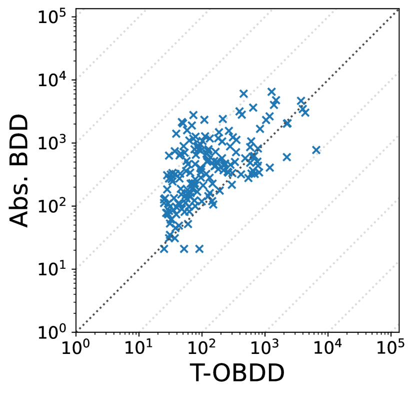
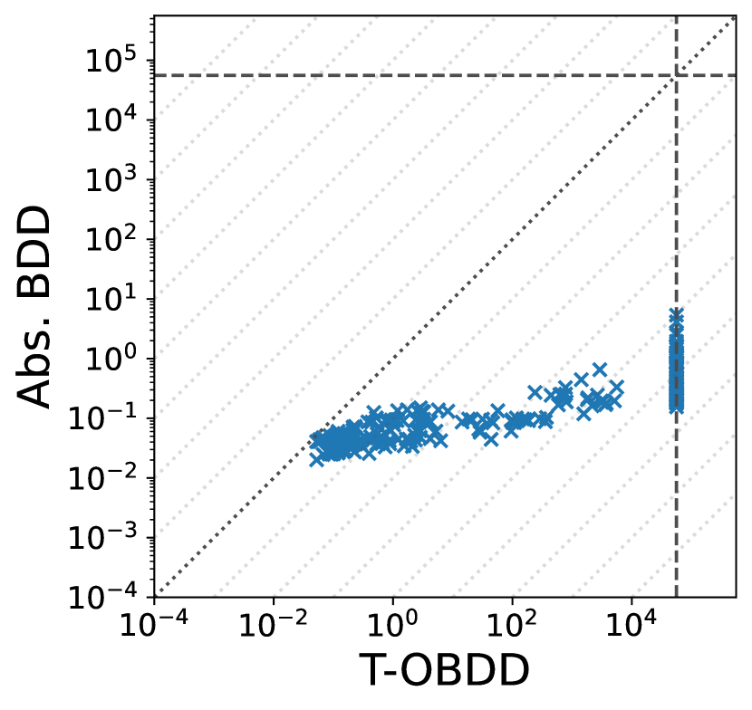
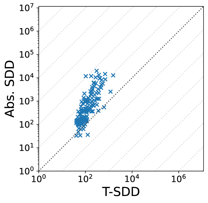
(a) Number of nodes

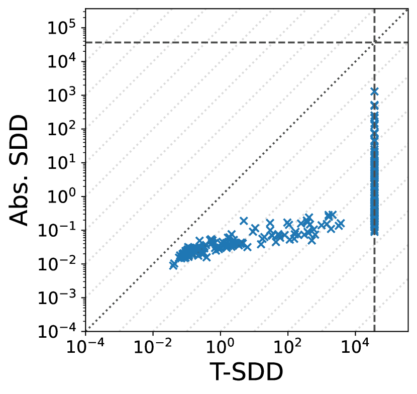
(b) Computational time

Figure 9: Results obtained on synthetic $\mathcal{LRA}$ benchmarks (250 problems), comparing number of nodes (left) and computational times (right). Timeouts on the horizontal and vertical lines. $\mathcal{T}$-OBDD timeouts: 79. $\mathcal{T}$-SDD timeouts: 111.

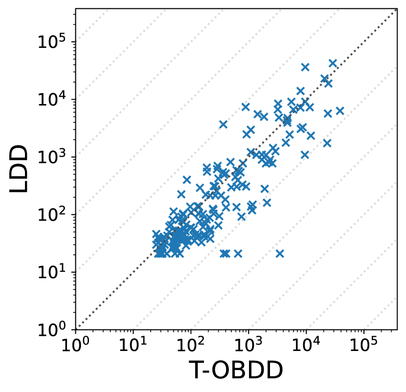
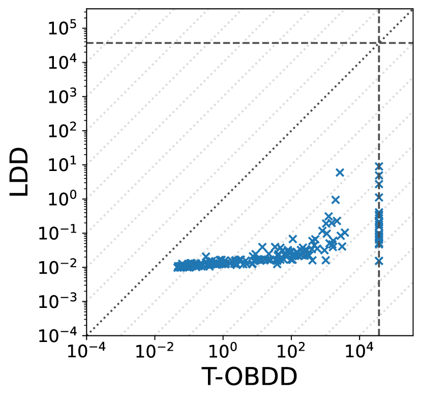
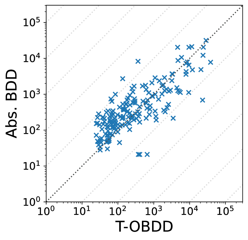
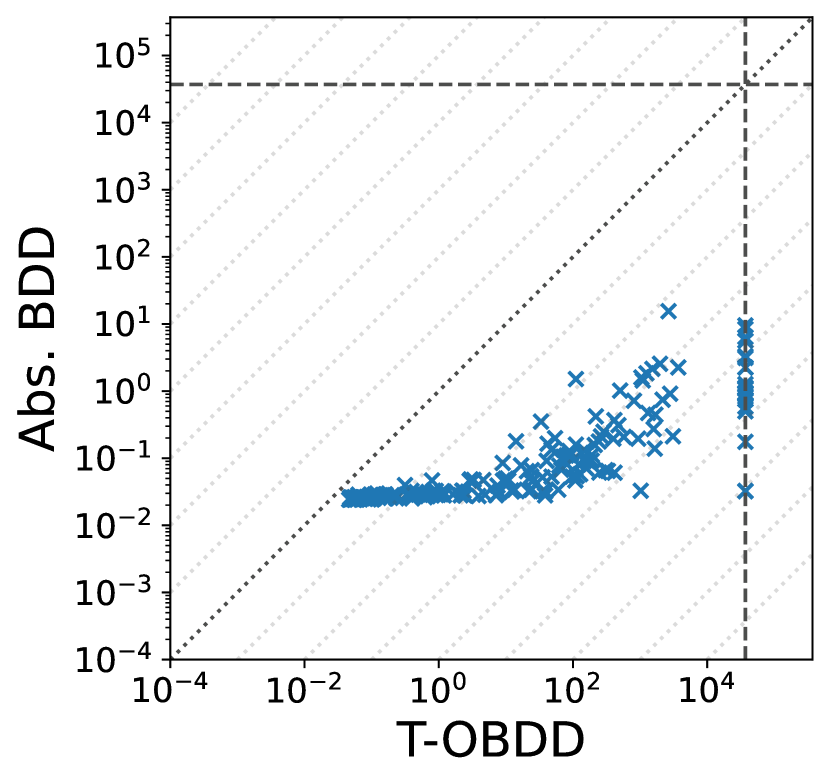
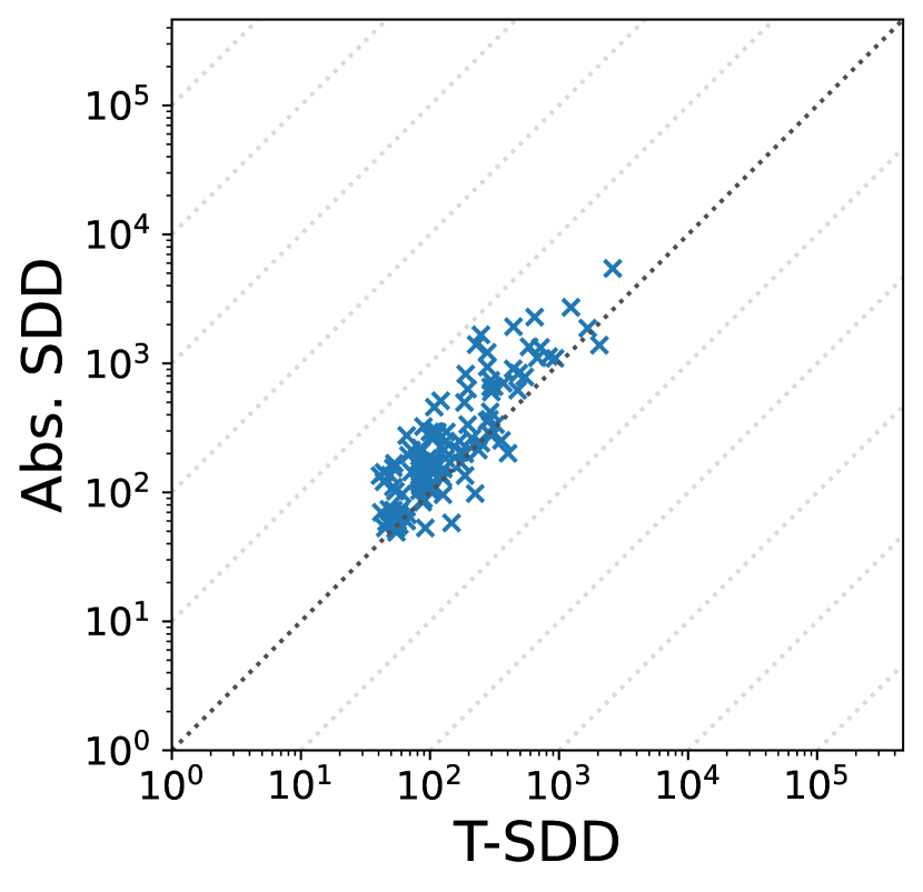
(a) Number of nodes

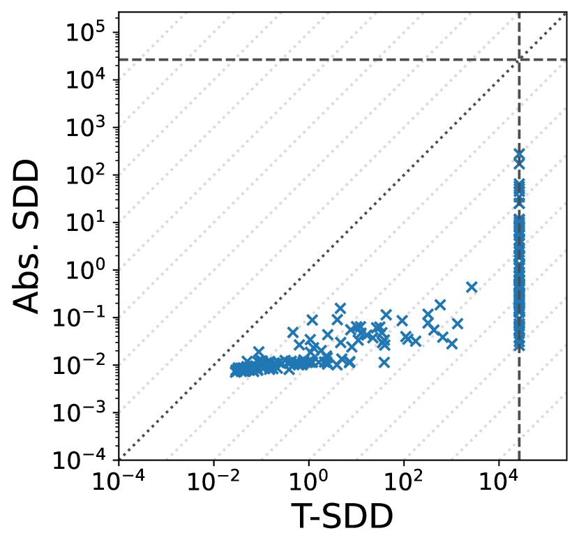
(b) Computational time

Figure 10: Results obtained on synthetic $\mathcal{TVPI}$ benchmarks (200 problems), comparing number of nodes (left) and computational times (right). Timeouts on the horizontal and vertical lines. LDD timeouts: 0. $\mathcal{T}$-OBDD timeouts: 22. $\mathcal{T}$-SDD timeouts: 81.

5.3 Results

Figures 9 and 10 show the comparison of our algorithm ($x$-axis) against all baseline solvers ($y$-axis). The results are shown through scatter plots, comparing the size of the generated $\mathcal{T}$-DDs and the taken computational time. We set the timeout to 3600s for AllSMT computation, and additional 3600s for $\mathcal{T}$-DD generation. Notice that both axes are log-scaled. On the one hand, the plots show that our algorithms have longer computational times compared to the other tools. This outcome is not surprising, given the additional overhead associated with enumerating the lemmas via AllSMT and performing Boolean existential quantification. On the other hand, our tools generate smaller $\mathcal{T}$-DDs, which is particularly noticeable for $\mathcal{T}$-SDDs.

Our tools offer several distinctive advantages that set them apart within the field. Notably, these advantages may not be readily discernible from scatter plots or other visualization methods.

The $\mathcal{T}$-DDs built with our approach ensure that every extension of a partial assignment leading to the $\top$ node represents a $\mathcal{T}$-consistent total assignment. Consequently, our algorithm stands as the sole contender capable of performing #SMT, aligning with the definition of #SMT proposed in [31]. This characteristic holds substantial implications for various applications, particularly in fields like Quantitative Information Flow, where precise enumeration is crucial.

Furthermore, benchmarks from the SMT-LIB, predominantly comprising UNSAT instances, proved our capability to identify $\mathcal{T}$-inconsistent formulas and condense them into a single $\bot$ node. In contrast, LDD do not generate a $\bot$ $\mathcal{T}$-DD for these formulas, highlighting once again their lack in achieving $\mathcal{T}$-semicanonicity.

Finally, our algorithm supports the combination of theories and addresses theories not supported by other available implementations. In the tool repository, we provide a collection of problems spanning various theories, all of which are compatible with our implementation. Notably, our tool is the only one capable of generating theory decision diagrams for these problem domains.

6 Conclusions and Future Work

In this paper, we have investigated the problem of leveraging Boolean decision diagrams (DDs) to SMT level ($\mathcal{T}$-DDs). We have presented a general theory-agnostic and DD-agnostic formal framework for $\mathcal{T}$-DDs. We have shown a straightforward way to leverage DDs to $\mathcal{T}$-DDs by simply combining an AllSMT solver and a DD package, both used as black boxes. This approach requires little effort to implement, since it does not require to modify the code of the AllSMT solver and of the DD package, and is very general, since it can be applied to any theory supported by the AllSMT solver and combinations thereof, and to any DD with a compiler admitting Boolean existential quantification. Importantly, this technique has a fundamental feature: it allows leveraging canonical DDs into $\mathcal{T}$-canonical $\mathcal{T}$-DDs. To the best of our knowledge, this is the first case of provably canonical $\mathcal{T}$-DDs in the literature. We have implemented our approach on top of the MathSAT AllSMT solver and of both OBDD and SDD packages, and shown empirically its effectiveness.

This work opens several research avenues, and will progress along several directions. From a theoretical viewpoint, we are going to investigate how $\mathcal{T}$-DDs can be effectively composed and how querying can be performed; also, we plan to extend our analysis to other forms of DDs, and on NNF formulas in general (in particular d-DNNF), investigating how their properties can be preserved by leveraging to SMT level. From a practical viewpoint, our approach currently suffers from two main bottlenecks: (a) the need to perform AllSMT upfront and (b) the need to perform Boolean existential quantification to remove the extra $\mathcal{T}$-atoms. For the former, we plan to investigate alternative and less-expensive ways to enumerate $\mathcal{T}$-lemmas ruling out $\mathcal{T}$-inconsistent assignments. For the latter, we plan to investigate alternative SMT techniques which reduce or even eliminate the presence of novel $\mathcal{T}$-atoms in the $\mathcal{T}$-lemmas. From an application viewpoint, we plan to use our $\mathcal{T}$-SDDs package for Weighted Model Integration (WMI), with the idea of merging the best features of AllSMT-based WMI [33] and those of KC-based WMI [20, 28].

Appendix A Appendix: Proofs of the theorems

Proof of Theorem 3

Proof.

Let $\Psi[{\boldsymbol{\alpha}}]\stackrel{{\scriptstyle\text{\scalebox{0.7}{def}}}}{{=}}\textrm{$\mathcal{T}$-DD}{(\varphi[{\boldsymbol{\alpha}}])}$ and $\Psi^{\prime}[{\boldsymbol{\alpha}}]\stackrel{{\scriptstyle\text{\scalebox{0.7}{def}}}}{{=}}\textrm{$\mathcal{T}$-DD}{(\varphi^{\prime}[{\boldsymbol{\alpha}}])}$. Then $\Psi[{\boldsymbol{\alpha}}]=\Psi^{\prime}[{\boldsymbol{\alpha}}]$ if and only if $\Psi^{p}[{\boldsymbol{\alpha}}]=\Psi^{\prime p}[{\boldsymbol{\alpha}}]$. By Definition 1, $\Psi^{p}[{\boldsymbol{\alpha}}]$ and $\Psi^{\prime p}[{\boldsymbol{\alpha}}]$ are DDs, which are canonical by hypothesis. Thus $\Psi^{p}[{\boldsymbol{\alpha}}]=\Psi^{\prime p}[{\boldsymbol{\alpha}}]$ if and only if $\Psi^{p}[{\boldsymbol{\alpha}}]\equiv\Psi^{\prime p}[{\boldsymbol{\alpha}}]$, that is, if and only if $\Psi[{\boldsymbol{\alpha}}]\equiv_{\mathbb{B}}\Psi^{\prime}[{\boldsymbol{\alpha}}]$. ∎

Proof of Theorem 5

Proof.

Consider two $\text{SMT}(\mathcal{T})$ formulas $\varphi[{\boldsymbol{\alpha}}]$ and $\varphi^{\prime}[{\boldsymbol{\alpha}}]$.
By Proposition 1(d), $\varphi[{\boldsymbol{\alpha}}]\equiv_{\mathcal{T}}\varphi^{\prime}[{\boldsymbol{\alpha}}]$ if and only if $H_{{\boldsymbol{\alpha}}}(\varphi{})=H_{{\boldsymbol{\alpha}}}(\varphi^{\prime}{})$.
By the definition of $H_{{\boldsymbol{\alpha}}}(...)$ all the $\eta{}$s in $H_{{\boldsymbol{\alpha}}}(...)$ are total on ${\boldsymbol{\alpha}}$ and pairwise disjoint, so that $H_{{\boldsymbol{\alpha}}}(\varphi{})=H_{{\boldsymbol{\alpha}}}(\varphi^{\prime}{})$ if and only if $\bigvee_{\eta_{i}\in H_{{\boldsymbol{\alpha}}}(\varphi{})}\eta_{i}\equiv_{\mathbb{B}}\bigvee_{\eta^{\prime}_{i}\in H_{{\boldsymbol{\alpha}}}(\varphi^{\prime}{})}\eta^{\prime}_{i}$.
Since $\textrm{$\mathcal{T}$-DD}{(\varphi[{\boldsymbol{\alpha}}])}\equiv_{\mathbb{B}}\bigvee_{\eta_{i}\in H_{{\boldsymbol{\alpha}}}(\varphi{})}\eta_{i}$ and $\textrm{$\mathcal{T}$-DD}{(\varphi^{\prime}[{\boldsymbol{\alpha}}])}\equiv_{\mathbb{B}}\bigvee_{\eta^{\prime}_{i}\in H_{{\boldsymbol{\alpha}}}(\varphi^{\prime}{})}\eta^{\prime}_{i}$, then we have that $H_{{\boldsymbol{\alpha}}}(\varphi{})=H_{{\boldsymbol{\alpha}}}(\varphi^{\prime}{})$ if and only if $\textrm{$\mathcal{T}$-DD}{(\varphi[{\boldsymbol{\alpha}}])}\equiv_{\mathbb{B}}\textrm{$\mathcal{T}$-DD}{(\varphi^{\prime}[{\boldsymbol{\alpha}}])}$.
By Theorem 3, $\textrm{$\mathcal{T}$-DD}{(\varphi[{\boldsymbol{\alpha}}])}\equiv_{\mathbb{B}}\textrm{$\mathcal{T}$-DD}{(\varphi^{\prime}[{\boldsymbol{\alpha}}])}$ if and only if $\textrm{$\mathcal{T}$-DD}{(\varphi[{\boldsymbol{\alpha}}])}=\textrm{$\mathcal{T}$-DD}{(\varphi^{\prime}[{\boldsymbol{\alpha}}])}$. ∎

Proof of Theorem 6

Proof.

Theorem 6 is a corollary of Theorem 8 (which we prove below) by setting ${\boldsymbol{\beta}}\stackrel{{\scriptstyle\text{\scalebox{0.7}{def}}}}{{=}}\emptyset$. ∎

Proof of Theorem 7

Proof.

Theorem 7 is a corollary of Theorem 11 (which we prove below) by setting ${\boldsymbol{\beta}}\stackrel{{\scriptstyle\text{\scalebox{0.7}{def}}}}{{=}}\emptyset$. ∎

Proof of Theorem 8

Proof.

Since $Cl_{{\boldsymbol{\alpha}},{\boldsymbol{\beta}}}(\varphi)$ rules out $P_{{\boldsymbol{\alpha}}}(\varphi)$, we have:

$$\bigvee\limits_{\rho_{j}[{\boldsymbol{\alpha}}]\in P_{{\boldsymbol{\alpha}}}(\varphi)}\rho_{j}[{\boldsymbol{\alpha}}]\ \wedge\ \bigwedge_{C_{l}[{\boldsymbol{\alpha}},{\boldsymbol{\beta}}]\in Cl_{{\boldsymbol{\alpha}},{\boldsymbol{\beta}}}(\varphi)}C_{l}[{\boldsymbol{\alpha}},{\boldsymbol{\beta}}]\ \equiv_{\mathbb{B}}\ \bot,$$ (9)

i.e.: $$\bigvee\limits_{\rho_{j}[{\boldsymbol{\alpha}}]\in P_{{\boldsymbol{\alpha}}}(\varphi)}\rho_{j}^{p}[{\boldsymbol{A}}]\ \wedge\ \bigwedge\limits_{C_{l}[{\boldsymbol{\alpha}},{\boldsymbol{\beta}}]\in Cl_{{\boldsymbol{\alpha}},{\boldsymbol{\beta}}}(\varphi)}C_{l}^{p}[{\boldsymbol{A}},{\boldsymbol{B}}]\ \equiv\ \bot,$$ (10)

equiv.: $$\bigvee\limits_{\rho_{j}[{\boldsymbol{\alpha}}]\in P_{{\boldsymbol{\alpha}}}(\varphi)}\rho_{j}^{p}[{\boldsymbol{A}}]\ \wedge\ \exists{\boldsymbol{B}}.\bigwedge\limits_{C_{l}[{\boldsymbol{\alpha}},{\boldsymbol{\beta}}]\in Cl_{{\boldsymbol{\alpha}},{\boldsymbol{\beta}}}(\varphi)}C_{l}^{p}[{\boldsymbol{A}},{\boldsymbol{B}}]\ \equiv\ \bot$$ (11)

Let $\varphi^{*p}[{\boldsymbol{A}}]\stackrel{{\scriptstyle\text{\scalebox{0.7}{def}}}}{{=}}\exists{\boldsymbol{B}}.\bigwedge_{C_{l}[{\boldsymbol{\alpha}},{\boldsymbol{\beta}}]\in Cl_{{\boldsymbol{\alpha}},{\boldsymbol{\beta}}}(\varphi)}C_{l}^{p}[{\boldsymbol{A}},{\boldsymbol{B}}]$. Since the $\eta_{i}[{\boldsymbol{\alpha}}]$s in $H_{{\boldsymbol{\alpha}}}(\varphi)$ are all total on ${\boldsymbol{\alpha}}$, then for each $\eta_{i}[{\boldsymbol{\alpha}}]$, either $\eta_{i}^{p}[{\boldsymbol{A}}]\models\varphi^{*p}[{\boldsymbol{A}}]$ or $\eta_{i}^{p}[{\boldsymbol{A}}]\models\neg\varphi^{*p}[{\boldsymbol{A}}]$. The latter is not possible, because it would mean that $\eta_{i}^{p}[{\boldsymbol{A}}]\wedge\varphi^{*p}[{\boldsymbol{A}}]\models\bot$, and hence, by (11), $\eta{}\in P_{{\boldsymbol{\alpha}}}(\varphi)$, which would contradict the fact that $H_{{\boldsymbol{\alpha}}}(\varphi)$ and $P_{{\boldsymbol{\alpha}}}(\varphi)$ are disjoint. Thus we have:

$$\bigvee_{\eta_{i}[{\boldsymbol{\alpha}}]\in H_{{\boldsymbol{\alpha}}}(\varphi)}\eta_{i}^{p}[{\boldsymbol{A}}]\models\exists{\boldsymbol{B}}.\bigwedge_{C_{l}[{\boldsymbol{\alpha}},{\boldsymbol{\beta}}]\in Cl_{{\boldsymbol{\alpha}},{\boldsymbol{\beta}}}(\varphi)}C_{l}^{p}[{\boldsymbol{A}},{\boldsymbol{B}}].$$ (12)

Hence, we have that:

$$\varphi_{\ }^{p}[{\boldsymbol{A}}]\wedge\exists{\boldsymbol{B}}.\bigwedge_{C_{l}[{\boldsymbol{\alpha}},{\boldsymbol{\beta}}]\in Cl_{{\boldsymbol{\alpha}},{\boldsymbol{\beta}}}(\varphi)}C_{l}^{p}[{\boldsymbol{A}},{\boldsymbol{B}}]\$$

by (1): $$\equiv \left(\bigvee_{\eta_{i}[{\boldsymbol{\alpha}}]\in H_{{\boldsymbol{\alpha}}}(\varphi)}\eta_{i}^{p}[{\boldsymbol{A}}]\ \vee\ \bigvee_{\rho_{j}[{\boldsymbol{\alpha}}]\in P_{{\boldsymbol{\alpha}}}(\varphi)}\rho_{j}^{p}[{\boldsymbol{A}}]\right)\wedge$$ (13)

$$\exists{\boldsymbol{B}}.\bigwedge_{C_{l}[{\boldsymbol{\alpha}},{\boldsymbol{\beta}}]\in Cl_{{\boldsymbol{\alpha}},{\boldsymbol{\beta}}}(\varphi)}C_{l}^{p}[{\boldsymbol{A}},{\boldsymbol{B}}]\$$

$$\wedge/\vee \equiv \left(\bigvee_{\eta_{i}[{\boldsymbol{\alpha}}]\in H_{{\boldsymbol{\alpha}}}(\varphi)}\eta_{i}^{p}[{\boldsymbol{A}}]\ \wedge\exists{\boldsymbol{B}}.\bigwedge_{C_{l}[{\boldsymbol{\alpha}},{\boldsymbol{\beta}}]\in Cl_{{\boldsymbol{\alpha}},{\boldsymbol{\beta}}}(\varphi)}C_{l}^{p}[{\boldsymbol{A}},{\boldsymbol{B}}]\right)\vee$$: (14)

$$\left(\bigvee_{\rho_{j}[{\boldsymbol{\alpha}}]\in P_{{\boldsymbol{\alpha}}}(\varphi)}\rho_{j}^{p}[{\boldsymbol{A}}]\wedge\exists{\boldsymbol{B}}.\bigwedge_{C_{l}[{\boldsymbol{\alpha}},{\boldsymbol{\beta}}]\in Cl_{{\boldsymbol{\alpha}},{\boldsymbol{\beta}}}(\varphi)}C_{l}^{p}[{\boldsymbol{A}},{\boldsymbol{B}}]\right)$$

by (11): $$\equiv \left(\bigvee_{\eta_{i}[{\boldsymbol{\alpha}}]\in H_{{\boldsymbol{\alpha}}}(\varphi)}\eta_{i}^{p}[{\boldsymbol{A}}]\ \wedge\exists{\boldsymbol{B}}.\bigwedge_{C_{l}[{\boldsymbol{\alpha}},{\boldsymbol{\beta}}]\in Cl_{{\boldsymbol{\alpha}},{\boldsymbol{\beta}}}(\varphi)}C_{l}^{p}[{\boldsymbol{A}},{\boldsymbol{B}}]\right)$$

by (12): $$\equiv \bigvee_{\eta_{i}[{\boldsymbol{\alpha}}]\in H_{{\boldsymbol{\alpha}}}(\varphi)}\eta_{i}^{p}[{\boldsymbol{A}}].$$

∎

Proof of Theorem 10

Proof.

By applying Theorem 8 to both $\varphi[{\boldsymbol{\alpha}}]$ and $\varphi^{\prime}[{\boldsymbol{\alpha}}]$ we obtain:

$$\varphi^{p}[{\boldsymbol{A}}]\wedge\exists{\boldsymbol{B}}.\bigwedge_{C_{l}[{\boldsymbol{\alpha}},{\boldsymbol{\beta}}]\in Cl_{{\boldsymbol{\alpha}},{\boldsymbol{\beta}}}(\varphi)}C_{l}^{p}[{\boldsymbol{A}},{\boldsymbol{B}}] \equiv \bigvee_{\eta_{i}[{\boldsymbol{\alpha}}]\in H_{{\boldsymbol{\alpha}}}(\varphi)}\eta_{i}^{p}[{\boldsymbol{A}}]$$ (15)

$$\varphi^{\prime p}[{\boldsymbol{A}}]\wedge\exists{\boldsymbol{B^{\prime}}{}}.\bigwedge_{C_{l}^{\prime}[{\boldsymbol{\alpha}},{\boldsymbol{\beta^{\prime}}}]\in Cl_{{\boldsymbol{\alpha}},{\boldsymbol{\beta^{\prime}}}}(\varphi^{\prime})}C_{l}^{\prime p}[{\boldsymbol{A}},{\boldsymbol{B^{\prime}}{}}] \equiv \bigvee_{\eta_{i}^{\prime}[{\boldsymbol{\alpha}}]\in H_{{\boldsymbol{\alpha}}}(\varphi^{\prime})}\eta_{i}^{\prime p}[{\boldsymbol{A}}].$$ (16)

By Property 1(d), $\varphi[{\boldsymbol{\alpha}}]\equiv_{\mathcal{T}}\varphi^{\prime}[{\boldsymbol{\alpha}}]$ if and only if $H_{{\boldsymbol{\alpha}}}(\varphi)=H_{{\boldsymbol{\alpha}}}(\varphi^{\prime})$, that is, if and only if:

$$\bigvee_{\eta_{i}[{\boldsymbol{\alpha}}]\in H_{{\boldsymbol{\alpha}}}(\varphi)}\eta_{i}^{p}[{\boldsymbol{A}}]\equiv\bigvee_{\eta_{i}^{\prime}[{\boldsymbol{\alpha}}]\in H_{{\boldsymbol{\alpha}}}(\varphi^{\prime})}\eta_{i}^{\prime p}[{\boldsymbol{A}}].$$ (17)

Thus, by combining (17) with (15) and (16), we have that $\varphi[{\boldsymbol{\alpha}}]\equiv_{\mathcal{T}}\varphi^{\prime}[{\boldsymbol{\alpha}}]$ if and only if (7) holds. ∎

Proof of Theorem 11

Proof.

Let $\varphi[{\boldsymbol{\alpha}}]$ and $\varphi^{\prime}[{\boldsymbol{\alpha}}]$ be $\mathcal{T}$-formulas. By Theorem 10, $\varphi[{\boldsymbol{\alpha}}]\equiv_{\mathcal{T}}\varphi^{\prime}[{\boldsymbol{\alpha}}]$ if and only if (7) holds. Since the DDs are canonical and ${\cal B}2{\cal T}$ is injective, (7) holds if and only if $\textrm{$\mathcal{T}$-DD}{}(\varphi[{\boldsymbol{\alpha}}])=\textrm{$\mathcal{T}$-DD}{}(\varphi^{\prime}[{\boldsymbol{\alpha}}])$. ∎

Appendix B Appendix: Extended Related Work

	Solver	Theory	Avail.	Prune inconsistent paths	Semi-canonical	Canonical
BDD	EQ-BDDs [23]	$\mathcal{E}$	*	✓	✓	✗
	Goel-FM [25, 26]	$\mathcal{E}$	✗	✓	✓	?
	Goel-$e_{ij}$ [25, 26]	$\mathcal{E}$	✗	✗	✗	✗
	Bryant [7]	$\mathcal{E}$	✗	✓	✓	?
	EUF-BDDs [34]	$\mathcal{EUF}$	*	✓	✓	✗
	(0,S,=)-BDDs [1, 2]	$\mathcal{E}\cup\{{0,S}\}$	✗	✓	✓	✗
	DDD [30]	$\mathcal{DL}$	✗	✓	✓	✗
	LDD [10]	$\mathcal{LA}$	✓	✗	✗	✗
	Chan [11]	$\mathcal{NLA}$	✗	✓	✗	✗
	haRVey [19]	any	✗	✓	✗	✗
	Fontaine [22]	any	✗	✓	✗	✗
	BDD+SMT [9, 13]	any	*	✓	✗	✗
SDD
	XSDD [20, 28]	$\mathcal{LRA}$	*	✗	✗	✗

Table 1: Theory-aware decision diagram solvers. The column Available indicates whether the solver is available for the given theory. The symbol “✓” means that the solver is publicly available, * means that the solver is implemented within another tool and not directly usable, and ✗ means that the solver is not publicly available. In the column Canonical, the symbol “?” indicates that the DDs may be canonical, but the authors do not provide a proof.

Several works have tried to leverage Decision Diagrams from the propositional to the SMT level. Most of them are theory-specific, in particular focusing on $\mathcal{E}$, $\mathcal{EUF}$ and (fragments of) arithmetic. $\mathcal{EUF}$-DDs are of particular interest in hardware verification [25, 26], while DDs for arithmetic have been mainly studied for the verification of infinite-state systems [11].

In the following, we present an analysis of the most relevant works that leverage DDs from the propositional to the SMT level. We focus on generalization of OBDDs and SDDs, as they are the most used DDs in the literature. In Table 1, we summarize the main properties of the analyzed works. From the table, we can see that most of the works are theory-specific, and while several $\mathcal{T}$-semicanonical DDs have been proposed, $\mathcal{T}$-canonical representations have been achieved only in some very-specific cases. With the only exception of LDDs [10], all the analyzed works do not have a public implementation or are implemented within other tools, making them not directly usable.

$\mathcal{T}$-DDs for $\mathcal{EUF}$.

In Goel et al. [25, 26], the authors describe two techniques to build OBDDs for the theory of equality ($\mathcal{E}$). The first consists in encoding each of the $n$ variables with $\lceil\log(n)\rceil$ bits, reducing to a Boolean formula. The resulting OBDD is, therefore, canonical, but its size is unmanageable even for small instances. The second approach consists in introducing a Boolean atom $e_{ij}$ for each equality $x_{i}=x_{j}$, and building a OBDD over these atoms. This essentially builds the OBDD of the Boolean abstraction of the formula, which allows for theory-inconsistent paths. This problem has been addressed in Bryant and Velev [7], where transitivity lemmas are instantiated in advance and conjoined with the OBDD. This approach is similar in flavour to our approach, and produces OBDDs whose refinement is $\mathcal{EUF}$-canonical; the main difference is that the procedure used to generate the lemmas is specific to the theory of equality, whereas our approach is general and can be applied to any theory supported by the SMT solver.

EQ-BDDs [23] extend OBDDs to allow for nodes with atoms representing equation between variables. EUF-BDDs [34] extend EQ-BDDs to atoms involving also uninterpreted functions. (0,S,=)-BDDs [1, 2] extend EQ-BDDs to atoms involving also the zero constant and the successor function. In all three cases, rewriting rules are applied to prune inconsistent paths. The resulting OBDDs are $\mathcal{T}$-semicanonical, but not $\mathcal{T}$-canonical.

$\mathcal{T}$-DDs for arithmetic.

Difference Decision Diagrams (DDDs) [30] are a generalization of OBDDs to the theory of difference logic ($\mathcal{DL}$). The building procedure consists in first building the refinement of the OBDD of the Boolean abstraction of the formula, and then pruning inconsistent paths by applying local and path reductions. Local reductions are based on rewriting rules, leveraging implications between predicates to reduce redundant splitting. Path reductions prune inconsistent paths, both those going to the $\top{}$ and $\bot{}$ terminals. The resulting DDD is $\mathcal{T}$-semicanonical, as $\mathcal{T}$-valid and $\mathcal{T}$-inconsistent formulas are represented by the $\top{}$ and $\bot{}$ DDDs, respectively. In general, however, they are not $\mathcal{T}$-canonical, even for formulas on the same atoms. Some desirable properties are discussed, and they conjecture that DDDs with these properties are canonical.

LDDs [10] generalize DDDs to $\mathcal{LA}$ formulas. However, the implementation restricts to the theory of Two Variables Per Inequality ($\mathcal{TVPI}$) over real or integer variables. Moreover, only local reductions are applied, making them not even $\mathcal{T}$-semicanonical. Most importantly, not even contradictions are recognized.

In [11], a procedure is described to build $\mathcal{T}$-OBDDs for nonlinear arithmetic ($\mathcal{NLA}$). The procedure consists in building the refinement of the OBDD of the Boolean abstraction of the formula, and then using an (incomplete) quadratic constraint solver to prune inconsistent paths. As a result, the $\mathcal{T}$-OBDD is not $\mathcal{T}$-semi-canonical, since $\mathcal{T}$-valid formulas may have different representations.

To the best of our knowledge, XSDDs [20, 28] are the only tentative to extend SDDs to support first-order theories. XSDDs have been proposed in the context of Weighted Model Integration (WMI), and extend SDDs by allowing for atoms representing linear inequalities on real variables in decision nodes. However, they only propose to refine the SDD of the Boolean abstraction of the formula, without any pruning of inconsistent paths. Simplifications are only done at later stages during the WMI computation.

$\mathcal{T}$-DDs for arbitrary theories.

In [19], a general way has been proposed to build $\mathcal{T}$-OBDDs. The tool named haRVey first builds the refinement of the OBDD of the Boolean abstraction of the formula. Then, it looks for a $\mathcal{T}$-inconsistent path, from which it extracts a subset of $\mathcal{T}$-inconsistent constraints. The negation of this subset, which is a $\mathcal{T}$-lemma, is conjoined to the $\mathcal{T}$-OBDD to prune this and possibly other $\mathcal{T}$-inconsistent paths. The procedure is iterated until no inconsistent paths are found. Here, only the lemmas necessary to prune $\mathcal{T}$-inconsistent partial assignments satisfying the formula are generated, making the resulting $\mathcal{T}$-OBDD not $\mathcal{T}$-semicanonical, as $\mathcal{T}$-valid formulas may have different representations.

The technique described in [22] is similar, but it generalizes to combination of theories.

In [9], the authors propose a general method to build $\mathcal{T}$-OBDD by integrating an OBDD compiler with an $\text{SMT}(\mathcal{T})$ solver, which is invoked to check the consistency of a path during its construction. The approach was refined in [13], where the authors propose many optimizations to get a tighter integration of the SMT solver within the $\mathcal{T}$-OBDD construction. In both cases, all inconsistent paths are pruned, but the resulting $\mathcal{T}$-OBDD is not $\mathcal{T}$-semicanonical.

References

• Badban and van de Pol [2004] B. Badban and J. van de Pol. An Algorithm to Verify Formulas by means of (O,S,=)-BDDs. In Proceedings of the 9th Annual Computer Society of Iran Computer Conference, Tehran, Iran, 2004.
• Badban and van de Pol [2005] B. Badban and J. van de Pol. Zero, successor and equality in BDDs. Annals of Pure and Applied Logic, 133(1):101–123, May 2005. ISSN 0168-0072. 10.1016/j.apal.2004.10.005.
• Barrett et al. [2021] C. W. Barrett, R. Sebastiani, S. A. Seshia, and C. Tinelli. Satisfiability Modulo Theories. In Handbook of Satisfiability, volume 336, pages 1267–1329. IOS Press, 2 edition, 2021.
• Bova [2016] S. Bova. SDDs Are Exponentially More Succinct than OBDDs. Proceedings of the AAAI Conference on Artificial Intelligence, 30(1), Feb. 2016. ISSN 2374-3468. 10.1609/aaai.v30i1.10107.
• Broeck [2011] G. Broeck. On the completeness of first-order knowledge compilation for lifted probabilistic inference. Advances in Neural Information Processing Systems, 24, 2011.
• Bryant [1986] R. E. Bryant. Graph-Based Algorithms for Boolean Function Manipulation. IEEE Transactions on Computers, C-35(8):677–691, Aug. 1986. ISSN 1557-9956. 10.1109/TC.1986.1676819.
• Bryant and Velev [2002] R. E. Bryant and M. N. Velev. Boolean satisfiability with transitivity constraints. ACM Transactions on Computational Logic, 3(4):604–627, Oct. 2002. ISSN 1529-3785. 10.1145/566385.566390.
• Burch et al. [1992] J. R. Burch, E. M. Clarke, K. L. McMillan, D. L. Dill, and L. J. Hwang. Symbolic model checking: 1020 States and beyond. Information and Computation, 98(2):142–170, June 1992. ISSN 0890-5401. 10.1016/0890-5401(92)90017-A.
• Cavada et al. [2007] R. Cavada, A. Cimatti, A. Franzen, K. Kalyanasundaram, M. Roveri, and R. Shyamasundar. Computing Predicate Abstractions by Integrating BDDs and SMT Solvers. In Formal Methods in Computer Aided Design, pages 69–76, Nov. 2007. 10.1109/FAMCAD.2007.35.
• Chaki et al. [2009] S. Chaki, A. Gurfinkel, and O. Strichman. Decision diagrams for linear arithmetic. In Formal Methods in Computer Aided Design, pages 53–60, Nov. 2009. 10.1109/FMCAD.2009.5351143.
• Chan et al. [1997] W. Chan, R. Anderson, P. Beame, and D. Notkin. Combining constraint solving and symbolic model checking for a class of systems with non-linear constraints. In O. Grumberg, editor, Computer Aided Verification, Lecture Notes in Computer Science, pages 316–327, Berlin, Heidelberg, 1997. Springer. ISBN 978-3-540-69195-2. 10.1007/3-540-63166-6_32.
• Chavira and Darwiche [2008] M. Chavira and A. Darwiche. On probabilistic inference by weighted model counting. Artificial Intelligence, 172(6-7):772–799, 2008.
• Cimatti et al. [2010] A. Cimatti, A. Franzen, A. Griggio, K. Kalyanasundaram, and M. Roveri. Tighter integration of BDDs and SMT for Predicate Abstraction. In 2010 Design, Automation & Test in Europe Conference & Exhibition (DATE 2010), pages 1707–1712, Mar. 2010. 10.1109/DATE.2010.5457090.
• Cimatti et al. [2011] A. Cimatti, A. Griggio, and R. Sebastiani. Computing Small Unsatisfiable Cores in Satisfiability Modulo Theories. Journal of Artificial Intelligence Research, 40:701–728, Apr. 2011. ISSN 1076-9757. 10.1613/jair.3196.
• Cimatti et al. [2013a] A. Cimatti, A. Griggio, B. J. Schaafsma, and R. Sebastiani. A Modular Approach to MaxSAT Modulo Theories. In 16th International Conference on Theory and Applications of Satisfiability Testing, Lecture Notes in Computer Science, pages 150–165, Berlin, Heidelberg, July 2013a. Springer-Verlag. ISBN 978-3-642-39070-8. 10.1007/978-3-642-39071-5_12.
• Cimatti et al. [2013b] A. Cimatti, A. Griggio, B. J. Schaafsma, and R. Sebastiani. The MathSAT 5 SMT Solver. In Tools and Algorithms for the Construction and Analysis of Systems, TACAS’13., volume 7795 of LNCS, pages 95–109. Springer, 2013b.
• Darwiche [2011] A. Darwiche. SDD: A new canonical representation of propositional knowledge bases. In 22nd International Joint Conference on Artificial Intelligence, volume 2 of IJCAI’11, pages 819–826, Barcelona, Catalonia, Spain, July 2011. AAAI Press. ISBN 978-1-57735-514-4.
• Darwiche and Marquis [2002] A. Darwiche and P. Marquis. A knowledge compilation map. Journal of Artificial Intelligence Research, 17(1):229–264, Sept. 2002. ISSN 1076-9757.
• Deharbe and Ranise [2003] D. Deharbe and S. Ranise. Light-weight theorem proving for debugging and verifying units of code. In First International Conference onSoftware Engineering and Formal Methods, 2003.Proceedings., pages 220–228, Sept. 2003. 10.1109/SEFM.2003.1236224.
• Dos Martires et al. [2019] P. Z. Dos Martires, A. Dries, and L. De Raedt. Exact and Approximate Weighted Model Integration with Probability Density Functions Using Knowledge Compilation. Proceedings of the AAAI Conference on Artificial Intelligence, 33(01):7825–7833, July 2019. ISSN 2374-3468, 2159-5399. 10.1609/aaai.v33i01.33017825.
• Fierens et al. [2012] D. Fierens, G. V. d. Broeck, I. Thon, B. Gutmann, and L. De Raedt. Inference in probabilistic logic programs using weighted cnf’s. arXiv preprint arXiv:1202.3719, 2012.
• Fontaine and Gribomont [2002] P. Fontaine and E. P. Gribomont. Using BDDs with Combinations of Theories. In M. Baaz and A. Voronkov, editors, Logic for Programming, Artificial Intelligence, and Reasoning, Lecture Notes in Computer Science, pages 190–201, Berlin, Heidelberg, 2002. Springer. ISBN 978-3-540-36078-0. 10.1007/3-540-36078-6_13.
• Friso Groote and van de Pol [2000] J. Friso Groote and J. van de Pol. Equational Binary Decision Diagrams. In M. Parigot and A. Voronkov, editors, Logic for Programming and Automated Reasoning, Lecture Notes in Artificial Intelligence, pages 161–178, Berlin, Heidelberg, 2000. Springer. ISBN 978-3-540-44404-6. 10.1007/3-540-44404-1_11.
• Gario and Micheli [2015] M. Gario and A. Micheli. PySMT: A solver-agnostic library for fast prototyping of SMT-based algorithms. In SMT Workshop 2015, 2015.
• Goel et al. [1998] A. Goel, K. Sajid, H. Zhou, A. Aziz, and V. Singhal. BDD based procedures for a theory of equality with uninterpreted functions. In A. J. Hu and M. Y. Vardi, editors, Computer Aided Verification, Lecture Notes in Computer Science, pages 244–255, Berlin, Heidelberg, 1998. Springer. ISBN 978-3-540-69339-0. 10.1007/BFb0028749.
• Goel et al. [2003] A. Goel, K. Sajid, H. Zhou, A. Aziz, and V. Singhal. BDD Based Procedures for a Theory of Equality with Uninterpreted Functions. Formal Methods in System Design, 22(3):205–224, May 2003. ISSN 1572-8102. 10.1023/A:1022988809947.
• Huang et al. [2006] J. Huang et al. Combining knowledge compilation and search for conformant probabilistic planning. In ICAPS, pages 253–262, 2006.
• Kolb et al. [2020] S. Kolb, P. Z. D. Martires, and L. D. Raedt. How to Exploit Structure while Solving Weighted Model Integration Problems. In 35th Conference on Uncertainty in Artificial Intelligence, pages 744–754. PMLR, Aug. 2020.
• Lahiri et al. [2006] S. K. Lahiri, R. Nieuwenhuis, and A. Oliveras. SMT Techniques for Fast Predicate Abstraction. In Computer Aided Verification, pages 424–437, 2006. ISBN 978-3-540-37411-4.
• Møller et al. [1999] J. Møller, J. Lichtenberg, H. R. Andersen, and H. Hulgaard. Difference Decision Diagrams. In J. Flum and M. Rodriguez-Artalejo, editors, Computer Science Logic, Lecture Notes in Computer Science, pages 111–125, Berlin, Heidelberg, 1999. Springer. ISBN 978-3-540-48168-3. 10.1007/3-540-48168-0_9.
• Phan [2015] Q.-S. Phan. Model counting modulo theories. arXiv preprint arXiv:1504.02796, 2015.
• Somenzi [2009] F. Somenzi. Cudd: Cu decision diagram package-release 2.4. 0. University of Colorado at Boulder, 21, 2009.
• Spallitta et al. [2024] G. Spallitta, G. Masina, P. Morettin, A. Passerini, and R. Sebastiani. Enhancing smt-based weighted model integration by structure awareness. Artificial Intelligence, 328:104067, 2024.
• van de Pol and Tveretina [2005] J. van de Pol and O. Tveretina. A BDD-Representation for the Logic of Equality and Uninterpreted Functions. In J. Jȩdrzejowicz and A. Szepietowski, editors, Mathematical Foundations of Computer Science 2005, Lecture Notes in Computer Science, pages 769–780, Berlin, Heidelberg, 2005. Springer. ISBN 978-3-540-31867-5. 10.1007/11549345_66.
• Van den Broeck [2013] G. Van den Broeck. Lifted inference and learning in statistical relational models. PhD thesis, PhD thesis, KU Leuven, 2013.