COBRA - COnfidence score Based on shape Regression Analysis for method-independent quality assessment of object pose estimation from single images

Abstract

We present a generic algorithm for scoring pose estimation methods that rely on single image semantic analysis. The algorithm employs a lightweight putative shape representation using a combination of multiple Gaussian Processes. Each Gaussian Process (GP) yields distance normal distributions from multiple reference points in the object’s coordinate system to its surface, thus providing a geometric evaluation framework for scoring predicted poses. Our confidence measure comprises the average mixture probability of pixel back-projections onto the shape template. In the reported experiments, we compare the accuracy of our GP based representation of objects versus the actual geometric models and demonstrate the ability of our method to capture the influence of outliers as opposed to the corresponding intrinsic measures that ship with the segmentation and pose estimation methods.

1 Introduction

The recovery of object pose from single images is a problem that arises in a variety of applications in robotics and computer vision and constitutes a topic of ongoing scrutiny. In the case of rigid objects, it allows the estimation of the object’s 3D location and 3D orientation in the coordinate system of the camera, also referred to as the 6D object pose.With the recent developments in machine learning, neural network based solutions have demonstrated significant efficiency, particularly in terms of detecting the 6D pose of objects from a single image with respect to some latent representation of the corresponding templates, e.g. [23, 10, 28]. Several works provide comprehensive reviews of such methods (e.g. [13, 37]), usually categorizing 6D object pose estimation according to the prior information, the number of views and the type of methods exploited. Drawing from the outcomes of the BOP Challenges [32], it is notable that while deep learning methods exhibited inferior performance compared to classical methods in 2018, nowadays they dominate the field. Significant accuracy improvement was demonstrated between 2020 and 2023, with the average recall of the best performing method to increase from 0.69 in 2020 to 0.85 in 2023. Methods have evolved to exploit RGB and RGBD data, both appearance and geometric information, tackling the problem of multiple object instances in the scene, objects with weak textures and symmetries [10] and by generalizing to estimate the pose of unseen objects, addressing category-level 6d pose estimation in a fully [17] or a semi-supervised manner [16]. The evaluation of 6D pose estimation methods typically resides on an established offline procedure exploiting ground truth benchmark data and state of the art metrics. Though certain cases necessitate quantifying the uncertainty of the estimated 6D pose at runtime. The most prominent examples stem from robot grasping and manipulation tasks, in which perception-action loops are exploited. The primary challenge lies in delivering an online confidence score for the estimated 6D object pose before initiating the robot action, thus preemptively filtering out less accurate poses that may result in unsuccessful grasps. In this paper we address the aforementioned challenge for object pose methods estimated from a single image and with available 3D object models. An alternative lightweight 3D shape representation for the object is derived, modeled via mixtures of Gaussian Processes priors, and which is used to assess the likelihood of estimated 3D object points belonging to the surface of the object and derive a confidence metric during online execution.

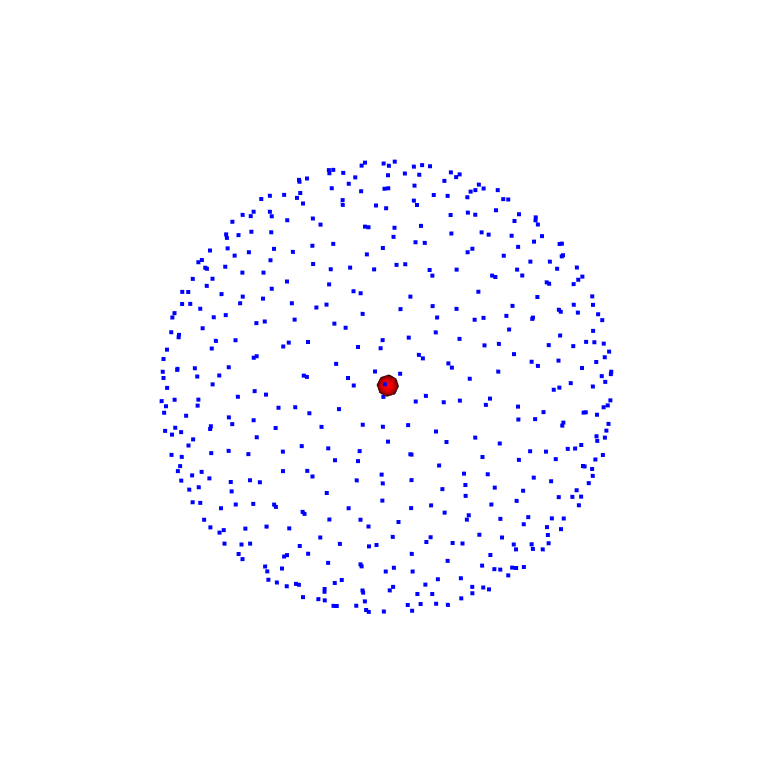
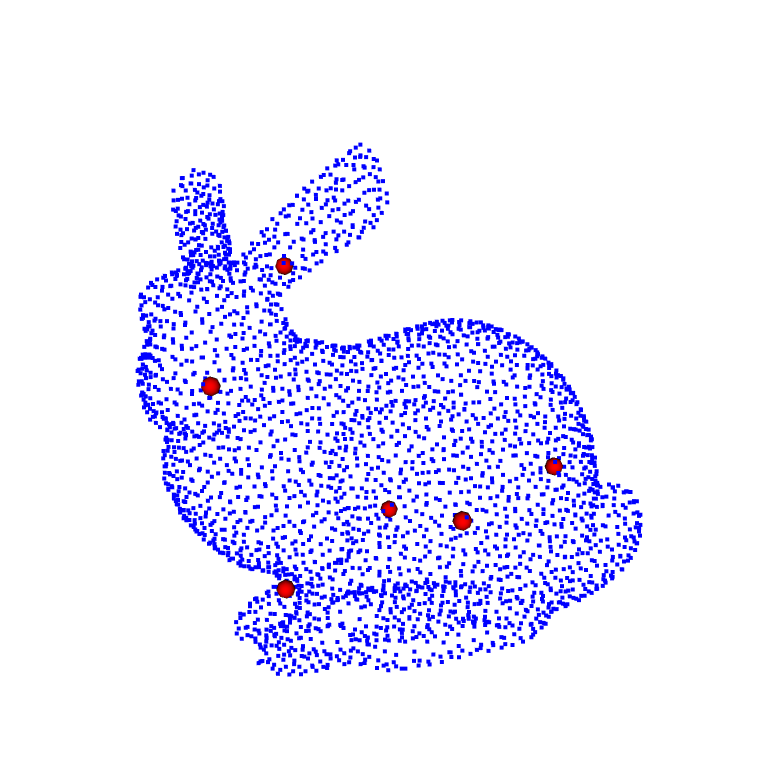
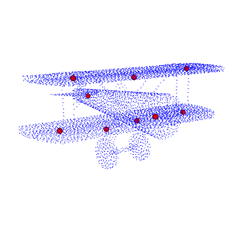
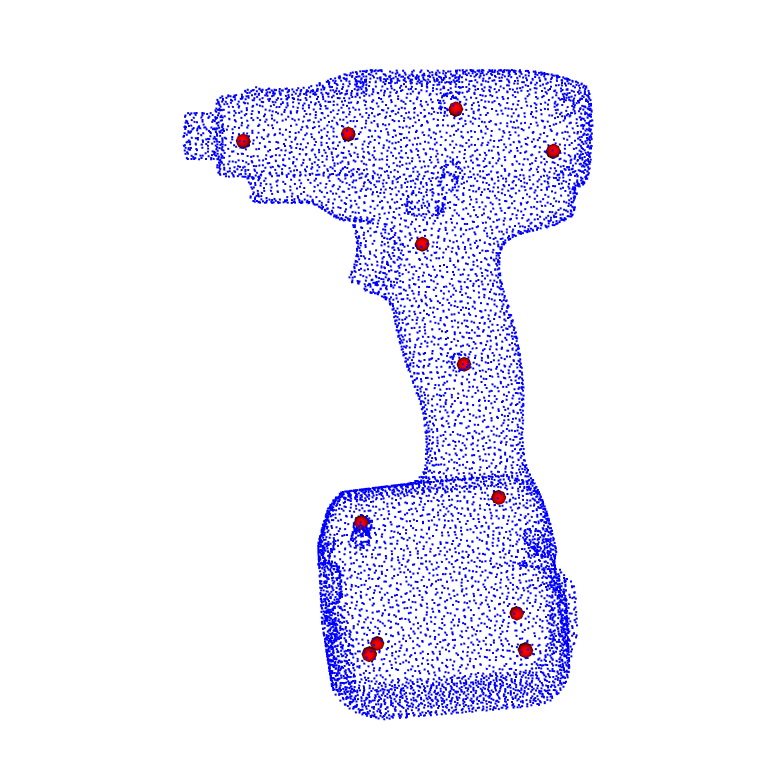
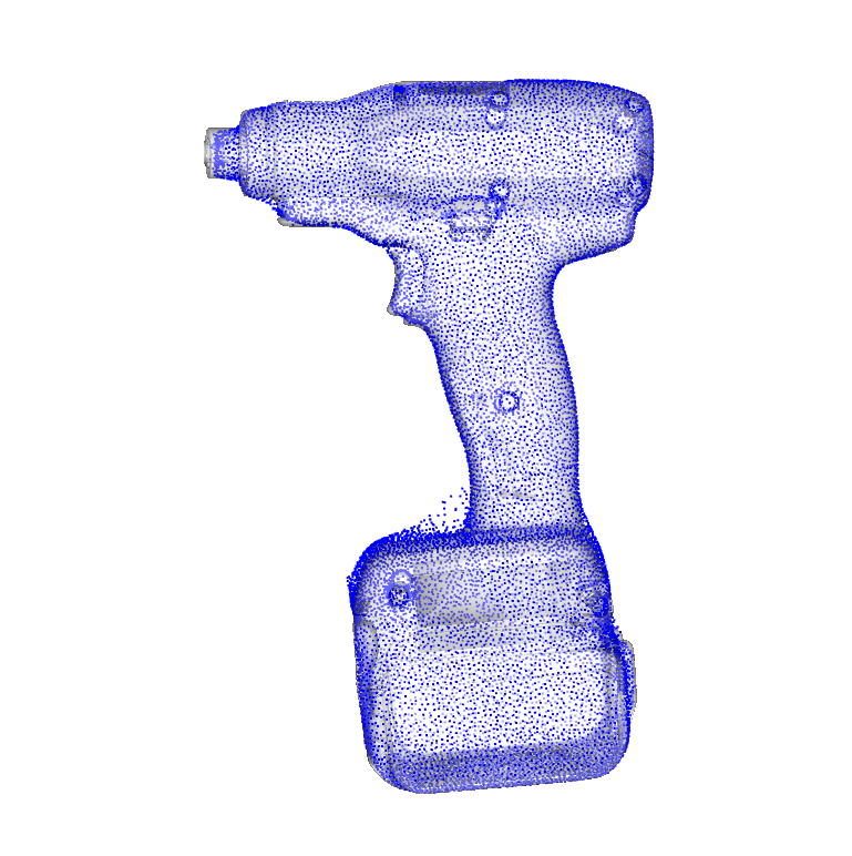
Figure 1: Shape reconstructions of objects with varying shape. Top row illustrates the training (blue) and reference (red) points (1, 2, 6, 9, 12). Bottom row shows the reconstructed 3D points from the trained Gaussian Processes with the ground truth object model (light gray) for comparison. Ratios of training/reconstructed points, 500/1500, 1000/3000, 3000/5000, 10K/20K, 10K/20K.

2 Contributions

We introduce a consistent, method-independent confidence measure for pose estimates relying on shape discrepancy in the local object coordinate frame. The contribution of our method is two-fold.

1. It provides a consistent and unbiased measure of quality for the pose estimate by assessing the consistency of the back-projected image of the object against an accurate shape template.

2. It leverages multiple GP based priors to obtain “lightweight” shape representations from sparse samples of the target (object) surface with sufficient accuracy to accommodate.

3 Related work

Related work focuses on the following areas: shape representation, 6D object pose evaluation and uncertainty estimation.

3.1 Shape representation

The representation of 3D shapes is a fundamental problem for various applications in 3D computer vision, prompting the exploration of different methodologies to encode object geometry. Explicit 3D representations, such as point clouds, meshes, and voxels, offer the ability to represent complex and arbitrary object shapes and shape details with simplicity but with increasing surface complexity the amount of data (i.e, points or vertices/faces) and the computation cost increases. While meshes, in comparison to points, can capture topology, their quality is contingent upon factors like resolution and the underlying topology. Implicit functions, encode shape priors and provide a continuous representation of shape, adept at handling complex topologies. With the advances in deep neural networks, learned shape representations have excelled and Farshian et al. [8] provide an extensive overview of related methods to date. These methods represent shape as either a learned feature vector, coupled with a trained decoder related to explicit representations such as point clouds [1, 27], meshes [35], voxels  [3], or represent shape with an implicit surface function. Deep implicit functions utilize an input observation as a latent vector and train a neural network to estimate binary occupancy [21] or a signed-distance function [25] at a given query location in 3D space, or model radiance/appearance properties of an object as seen in NeRF-based approaches [22]. Deep implicit functions have gained popularity and significantly advanced the state of the art in 3D shape generation [21, 25, 4, 9], 3D shape completion [5], 4D reconstruction [24], and 3D shape correspondence [18]. Several extensions have been proposed, including learning separate implicit functions for shape parts [26] or integrating a deformation model for shape registration [36]. While these methods generally provide compact shape representations with low dimensional latent vectors they encounter difficulties in representing the entirety of shapes, reconstructing details and generalizing to novel shape classes as often the implicit representation is hard to obtain due to the presence of noise and incomplete data points, while it is necessary to convert points and meshes to implicit distance fields.

On the other hand explicit representations complicate their deployment in deep learning due to their irregular (i.e. meshes) or even unordered (i.e. point clouds) nature of data types and existing works are either restricted to small deviations from a 3D template or graph or small number of vertices/ points or simple convex shapes restricted to limited output quality [8, 15]. Gaussian processes (GP) [29] is a promising modeling framework to encode information about object shape[7]. Objects can be represented as collections of points in space, which can be used as inputs to the GP model. These allow the specification of a prior distribution which can capture beliefs about the type of shapes, shape predictions and related uncertainty estimates of those predictions.

3.2 6D pose evaluation and uncertainty estimation

The standard approach adopted in the literature for evaluating solely the performance of 6D pose estimation methods is performed offline and relies on available benchmark ground truth data and state of the art metrics such as VSD, MSSD, MSPD, ADD [11] or 3-D IoU [34]. When 6D pose estimation is exploited in actionable tasks, i.e. perception-to-action robotic tasks, such as grasping, the grasps success rates are commonly computed. The object(s) are randomly placed and the grasping task is performed a number of times to measure the number of successful grasps. Though when it comes to prune less accurate poses that may lead to unsuccessful grasping during runtime and prior to any robot action a confidence measure for the pose estimation can serve this purpose. Related works fall under the broader research area of uncertainty quantification in robotics, especially the specific type of predictive uncertainty which reflects the risk of certain pose estimation. The majority of works along this research strand aim to endow deep pose estimation models with the capability to directly assess and quantify the uncertainty of their own predictions by directly training the model to output a confidence score [33, 20]. Though this set of approaches bears the challenge that the uncertainty is difficult to evaluate as the performance varies with respect to different input images, as there may be a large gap to the training data and ground truth data are unknown, therefore difficult to quantify. In principle they have the drawback of exhibiting limited robustness [2], bias to overfitting yielding overconfident estimates [31] and a deviation with the true uncertainty is often observable, while they tend to be computationally expensive. The method of [31] exploits ensemble methods [14], which in general tend to be more lightweight in terms of inference time. In [31] the problem is approached by an ensemble of different models with translational/rotational/ADD disagreement metrics and computing their average disagreement against one another as the uncertainty quantification. Although the method doesn’t require any modification of the training procedure or the model input, still inference time increases with the number of the different models used.

4 Method

The core idea of our method is to use putative 3D representations of objects (henceforth referred to as “templates”) that we are anticipating our classifier to detect and subsequently predict their pose. These classifiers typically ship with measures of self-assessed confidence that provide some indication of quality for the estimated pose. However, these quality measures bear the inherent bias of the self-assessment process and can therefore be misleading for the back-end application. To eliminate this bias, we resort to the use of lightweight object templates to validate the geometric consistency of the estimated object pose. Put differently, we utilize the pose estimate to generate a partial 3D reconstruction of the detected object and establish a confidence score by assessing the deviations of the reconstructed points from the template surface.

4.1 Shape representation with Gaussian processes

As discussed earlier in sec. 3.1 3D objects can be represented with pointclouds or meshes. With the former, large numbers of points are required, usually in the order of 100,000 or more, whereas the latter are significantly more lightweight, but with occasional loss of detail in surface regions represented by large polygons. The shortcomings of these representations with respect to the task at hand, i.e., the comparison between the reconstructed object against a template shape pertain to storage and time complexity that such a comparison entails. In particular, where point clouds are concerned, to evaluate the distance of a given point from the surface would require nearest neighbor queries for a large number of points, which, in turn, requires a large storage (e.g., a KD-tree) of tightly spaced points. Similarly, for mesh representations, such a query would require the determination of the polygon nearest to the given point, thereby incurring substantial spatial search.

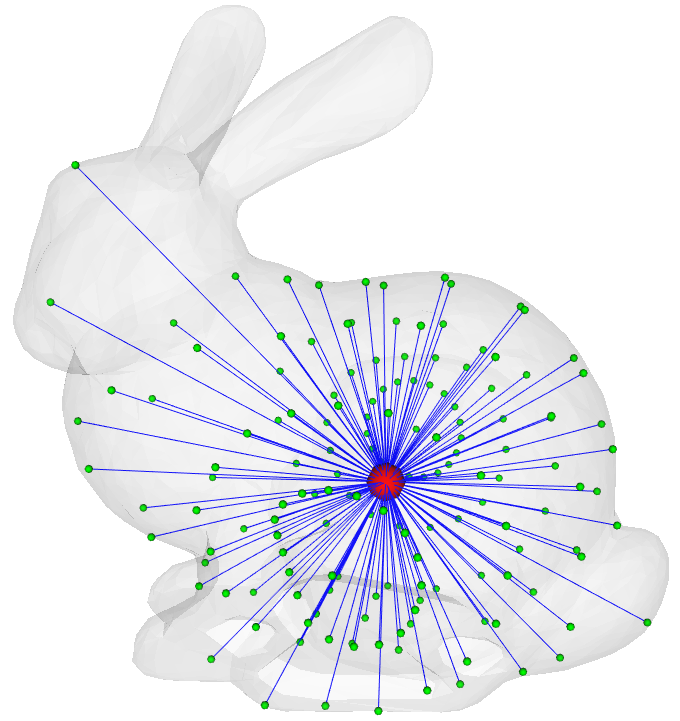
Figure 2: Parameterizing surface points $\boldsymbol{P}$ (green) as direction and distance (blue rays) w.r.t a reference point $\boldsymbol{C}$ (red)

4.1.1 Encoding 3D points with direction and distance.

To circumvent the aforementioned shortcomings, we resort to a functional representation of shape by means of a directional encoding from specially chosen reference points in the object’s local coordinate frame. Consider a reference point $\boldsymbol{C}$ in the object’s local frame and a given point $\boldsymbol{P}$ on the object’s surface. We parametrize $\boldsymbol{P}-\boldsymbol{C}$ in terms of its distance and direction from $\boldsymbol{C}$ (See Fig. 2) as follows:

$$\boldsymbol{P}-\boldsymbol{C}\coloneq\left(\phi,\theta,d\right)$$ (1)

where $\phi,\theta$ are the spherical coordinates of $\boldsymbol{P}-\boldsymbol{C}$ and $d=\|\boldsymbol{P}-\boldsymbol{C}\|$. Thus, if $\boldsymbol{u}(\phi,\theta)\in\mathbb{R}^{3}$ is the bearing vector defined by the spherical coordinates $\phi$ and $\theta$, we may obtain $\boldsymbol{P}$ as,

$$\boldsymbol{P}=d\,\boldsymbol{u}(\phi,\theta)+\boldsymbol{C}$$ (2)

The distance-direction parametrization of eqs. (1), (2), bears a two-fold benefit. For a given reference point, $\boldsymbol{C}$, in the interior of an object represented by a closed surface, we may represent all or part of the surface as a collection of distances along every possible direction from $\boldsymbol{C}$. Moreover, learning distances from directions is suitable for regression models.

4.1.2 Predicting distance to object surface with Gaussian processes.

Consider an object with an exterior surface that comprises points reachable by means of ray-casting from a point, $\boldsymbol{C}$, in the interior of the object. To fit this surface to a function, we model the random variables of distances from $\boldsymbol{C}$ to the surface along a given direction $\boldsymbol{u}(\phi,\theta)$, as a Gaussian process,

$$d\sim\mathcal{GP}\left(0,k\right),\;\;\text{s.t.}\;\;k:\left([0,\pi]\times[0,2\pi]\right)^{2}\rightarrow\mathbb{R}$$ (3)

where $k$ is the so-called covariance function mapping any two direction parameter vectors $\boldsymbol{\psi}=(\phi,\theta)$ and $\boldsymbol{\psi}^{\prime}=(\phi^{\prime},\theta^{\prime})$ to a real number, such that the Gram matrix $\boldsymbol{K}=\left[k(\boldsymbol{\psi}_{i},\boldsymbol{\psi}_{j})\right]$ is positive semi-definite (PSD) for any finite collection $\left\{\boldsymbol{\psi}_{1},\dots,\boldsymbol{\psi}_{n}\right\}$ of direction parameter vectors [29]. Different choices for the kernel $k$ give rise to different Gaussian processes. The Rational Quadratic (RQ) kernel, known for its capacity to regulate the extent of multi-scale behavior, stands out as a more adaptive option when compared to the Radial Basis Function (RBF) kernel [30, 29] and was found to work better in practice in our application:

$$k_{\mathrm{RQ}}(\boldsymbol{\psi}_{i},\boldsymbol{\psi}_{j})=\left(1+\frac{d_{ij}^{2}}{2\alpha l^{2}}\right)^{-\alpha},$$ (4)

where $l>0$, $\alpha>0$ are hyperparameters and $d_{ij}$ denotes the Euclidean distance, $\|\boldsymbol{\psi}_{i}-\boldsymbol{\psi}_{j}\|$, between the orientation parameters. Perhaps a more suitable choice for $d_{ij}$ would be the geodesic distance between the bearing vectors $\boldsymbol{u}(\boldsymbol{\psi}_{i})$, $\boldsymbol{u}(\boldsymbol{\psi}_{j})$, but that would lead to a non-PSD kernel function as shown in [12], to which a close valid alternative would be the Euclidean distance, $\|\boldsymbol{u}(\boldsymbol{\psi}_{i})-\boldsymbol{u}(\boldsymbol{\psi}_{j})\|$.

For a sufficiently sized training set of $n$ 3D points on the surface of the object, we may train the GP model to explicitly predict surface shape in terms of distance for given query directions from the point $\boldsymbol{C}$. Thus, via the GP prior, for a query direction parameter vector $\boldsymbol{x}\in\mathbb{R}^{2}$, we can obtain a conditional distribution over the distance to the surface along the given direction, and a collection of surface (training) data, $(\boldsymbol{\Psi},\boldsymbol{d})=\left(\left[\boldsymbol{\psi}_{1},\dots,\boldsymbol{\psi}_{M}\right],\left[d_{1},\dots,d_{M}\right]\right)$:

$$q\left(d|\ \boldsymbol{x},\boldsymbol{C};(\boldsymbol{\Psi},\boldsymbol{d})\right)\sim\mathcal{N}\left(\mu_{d|\boldsymbol{x}},\sigma^{2}_{d|\boldsymbol{x}}\right)$$ (5)

where,

$$\mu_{d|\boldsymbol{x}}=\boldsymbol{K}(\boldsymbol{x},\boldsymbol{\Psi})\boldsymbol{K}(\boldsymbol{\Psi},\boldsymbol{\Psi})^{-1}\boldsymbol{d},\;\;\sigma^{2}_{d|\boldsymbol{x}}=k(\boldsymbol{x},\boldsymbol{x})-\boldsymbol{K}(\boldsymbol{x},\boldsymbol{\Psi})\boldsymbol{K}(\boldsymbol{\Psi},\boldsymbol{\Psi})^{-1}\boldsymbol{K}(\boldsymbol{\Psi},\boldsymbol{x}).$$ (6)

To discharge notation, we will henceforth omit the training data from the likelihood expression, $q\left(d|\ \boldsymbol{x},\boldsymbol{C};(\boldsymbol{\Psi},d)\right)$, and simply use, $q\left(d|\ \boldsymbol{x},\boldsymbol{C}\right)$

Figure 3: Ray-casting to the objects’s surface (blue) from reference points (red) by retaining the first intersection. More dense coverage achieved with increasing number of reference points (left-to-right).

4.1.3 Surface coverage with mixtures of distance likelihoods

It becomes evident that for objects with more complex shapes, a single GP model will not suffice, because there would exist rays emanating from the reference point that intercept the exterior surface of the object in multiple points (e.g., Fig. 3). To cope with this issue, we introduce multiple reference points which we distribute preferably in the interior of the object in a way that achieves coverage of the entire surface. Interior reference points ensure that every direction corresponds to a valid training sample. A good strategy of obtaining such reference points would be distance-based clustering such as k-means  [19] or expectation maximization (EM) [6], because it will induce a surface partition that will comprise loosely convex patches that are fully reachable from the respective cluster centers via ray-casting. For each of these reference points, a new GP prior is introduced, therefore the complete object surface is modeled by training multiple predictors of local surface patches with reference points at the cluster centers.

Formally, the idea is to model the likelihood of a 3D point $\boldsymbol{P}$ belonging to the surface of the object $\boldsymbol{o}$ as a mixture of normal distributions derived from the corresponding GP priors with reference points at the cluster centers $\boldsymbol{C}_{k}$,

$$p(\boldsymbol{P}|\boldsymbol{o})=\sum_{k=1}^{K}p\left(\boldsymbol{P}|\boldsymbol{C}_{k};\boldsymbol{o}\right)\pi(\boldsymbol{C}_{k};\boldsymbol{o})$$ (7)

where we choose the likelihood $p\left(\boldsymbol{P}|\boldsymbol{C}_{k};\boldsymbol{o}\right)$ to be the GP prior based normal distribution of eq. (5), i.e.,

$$p\left(\boldsymbol{P}|\boldsymbol{C}_{k};\boldsymbol{o}\right)=q\left(\|\boldsymbol{P}-\boldsymbol{C}_{k}\|\,\big{|}\,\boldsymbol{x}_{P},\boldsymbol{C}_{k}\right),$$ (8)

and $\boldsymbol{x}_{P}$ is the direction parameter vector of $\boldsymbol{P}$ with respect to the reference point $\boldsymbol{C}_{k}$. Furthermore, the weighting probability $\pi(\boldsymbol{C}_{k};\boldsymbol{o})$ is modeled as a softmax ratio based on the distance of $\boldsymbol{P}$ from the reference point $\boldsymbol{C}_{k}$:

$$\pi(\boldsymbol{C}_{k};\boldsymbol{o})=\frac{\exp\left(-\left(\boldsymbol{P}-\boldsymbol{C}_{k}\right)^{T}\boldsymbol{Q}_{k}\left(\boldsymbol{P}-\boldsymbol{C}_{k}\right)\right)}{\sum_{l=1}^{K}\exp\left(-\left(\boldsymbol{P}-\boldsymbol{C}_{l}\right)^{T}\boldsymbol{Q}_{l}\left(\boldsymbol{P}-\boldsymbol{C}_{l}\right)\right)}$$ (9)

where $\boldsymbol{Q}_{k}$ is a covariance measure of the local space around the k-th cluster center (reference point) $\boldsymbol{C}_{k}$ . In practice, this means that we reconstruct a query point $\boldsymbol{P}$ by choosing the nearest center. This however can give rise to borderline errors in the assignment of query points to reference points. To cope with this problem, we impose inter-cluster overlap in the training (Fig. 4).

(a)

(b)

(c)

(d)

Figure 4: Classification of training points on the object surface without (a) and with cluster overlap in the blue areas (c). Reconstructed point clouds for each case of (a) and (c) in (b) and (d), respectively.

4.1.4 Distance likelihood based on test data

The primary goal of our templating technique with multiple GP priors is to obtain a fairly accurate shape representation of the object in question in order to use it as a putative surface to which we compare the back-projections of pixels in the image of the detected object with the estimated pose. Thus, the accuracy of the representation is crucial for the validity of the confidence score.

For our confidence computations, we choose in practice to employ a modified distance likelihood distribution,

$$\hat{q}\left(d|\ \boldsymbol{x},\boldsymbol{C};(\boldsymbol{\Psi},\boldsymbol{d})\right)\sim\mathcal{N}\left(\mu_{d|\boldsymbol{x}},\hat{\sigma}^{2}_{d|\boldsymbol{x}}\right),$$ (10)

where, as in eq. (5) the mean $\mu_{d|\boldsymbol{x}}$ is the GP prediction. However, noticing that the GP model tends to underestimate the variance of certain data points, we opted to replace ${\sigma}^{2}_{d|\boldsymbol{x}}$ with an estimate, $\hat{\sigma}^{2}_{d|\boldsymbol{x}}$, derived from actual (test) data.

4.2 Confidence scoring of pose estimates

The concept behind our confidence measure essentially relies on the discrepancy of the back-projections of classified pixels (belonging to a known object) from the corresponding object template surface via the estimated pose. Consider a classifier, trained to recognize objects from a pool set $\mathcal{O}$, captured in images, and to map the corresponding pixels $\boldsymbol{p}_{i}$ (belonging to an object $o\in\mathcal{O}$) to 3D points $\boldsymbol{P}_{i}$ in the object’s local coordinate frame. Also, let $\boldsymbol{T}\in\mathcal{SE}(3)$ be the pose prediction of the object by the classifier. Our confidence measure is the average weighted maximum probability of the back-projected points $\boldsymbol{P}_{i}$ in eq. (10) amongst all possible reference points

$$\mathcal{C}(\boldsymbol{T};o)=\sum_{i=1}^{N}w_{i}\left(\underset{k\in\left\{1,\dots,K\right\}}{\max}\hat{q}\left(\boldsymbol{P}_{i}|\boldsymbol{C}_{k};o\right)\right),$$ (11)

where $w_{i}$ is a weight (typically, a probability) that encapsulates the classifier’s self-assessed confidence about the quality of the pose estimate; clearly, if such a measure is not provided, then we choose $w_{i}=1/N$.

4.2.1 Associating confidence with absolute deviation in metric space

Since our confidence measure is an average probability by definition, we may obtain a link between a desired margin, $\delta$, pertaining to the distance of a back-projected image points to the surface of the object. Thus, if, for each back-projected point $\boldsymbol{P}_{i}$, the corresponding residual is bounded in absolute value by $\delta$, then we may obtain a lower bound for average confidence (for a proof refer to Appendix 0.A),

$$\overline{\mathcal{C}}\geq\frac{1}{\sqrt{2\pi}\delta^{2}}\sum_{i=1}^{N}w_{i}\hat{\sigma}_{d|\boldsymbol{x}}\left(1-\exp\left(-\frac{\delta^{2}}{2\hat{\sigma}_{d|\boldsymbol{x}}^{2}}\right)\right),$$ (12)

where $\hat{\sigma}_{d|\boldsymbol{x}}^{2}$ is the estimated variance as per section 4.1.4. With eq. (12) we are able to relate confidence values to a more tangible quantity such as distance.

5 Results

Objects	Metric	COBRA	DeepSDF (500k)	DeepSDF (10k)
Planes	CD Mean	0.9512	0.0146	0.0198
	CD Median	0.8246	0.0044	0.0069
Chairs	CD Mean	1.1616	0.0038	0.0036
	CD Median	1.1142	0.0036	0.0034
Sofas	CD Mean	1.5379	0.00919	0.0642
	CD Median	1.6411	0.00617	0.0322

Table 1: Comparison with DeepSDF trained with 500K and 10K points per object across shapes of varying complexity for the planes, chairs, and Sofas datasets from ShapeNet (5 models each). CD = Chamfer Distance (250K points) multiplied by $10^{2}$.

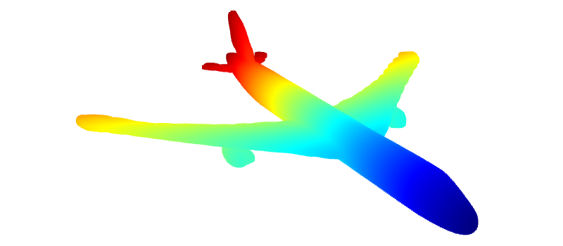
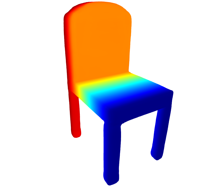
(a) Ground truth

(b) Ours

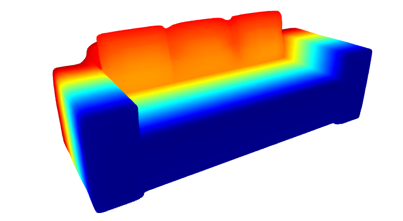
(c) DeepSDF [25]

Figure 5: Point cloud comparison between our method and DeepSDF.

Figure 6: Fidelity of wing and tail details achieved by each approach. From left to right: ground truth, ours, DeepSDF.

Our experimentation has dual scope: a) To assess the effectiveness of the confidence score in identifying a good pose and, b) to demonstrate the efficiency of the template. For the latter, we use various models from the ShapeNet dataset as well as objects from an industrial workspace wherein accurate robotic grasping of objects is a key operational feature.

5.1 Template accuracy, fidelity and comparative assessment

Table 1 shows the quantitative comparison and evaluation of the shape representation task against DeepSDF for known 3D shapes for the three different categories of the ShapeNet dataset namely planes, chairs, sofas. We employed 5 models from each of the mentioned categories to extract and assess the shape representation capabilities of the two methods using the Chamfer Distance (CD) for point cloud similarity. While, DeepSDF achieves better accuracy it is important to note that it is trained on the entire dataset of planes, chairs and sofas.

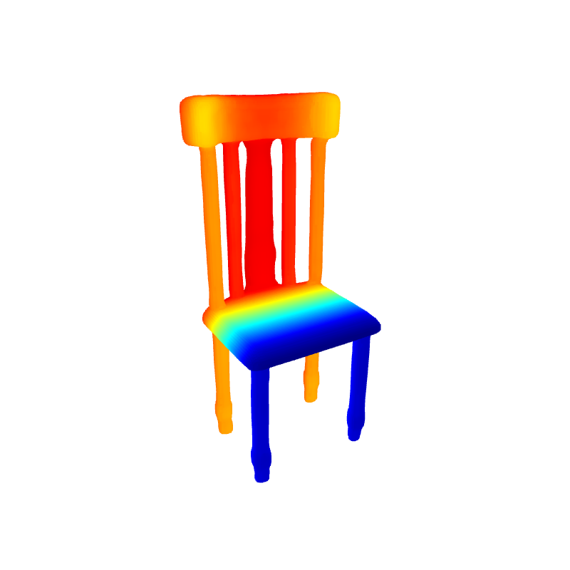
(a) Ground truth

(b) Ours (k-means)

(c) Ours (Manual)

(d) DeepSDF

Figure 7: (a) Ground truth, (b) Results obtained from automatically estimating reference point locations (16) with k-means, (c) Results based on manually defined reference points (32), (d) and DeepSDF result.

Fig. 5 illustrates reconstructions with our method and DeepSDF. Note that these are two intrinsically different methods. While DeepSDF excels in generalizing across different objects, our method is more adept in representing details of a specific object (Fig. 6). Clearly, the locations of the reference points may impact the fidelity of the template. Different approaches to determining these points might yield better results, particularly when dealing with complex objects. For instance, in the case of the chair depicted in Fig. 7, comparing results obtained from clustering-based estimation of reference points (cf. sect.  4.1) with those manually defined, a more accurate shape representation is derived. In the same figure, the results of DeepSDF for the same object are contrasted affirming the loss of object details.

5.2 Confidence as a measure of pose quality

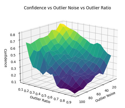
(a)

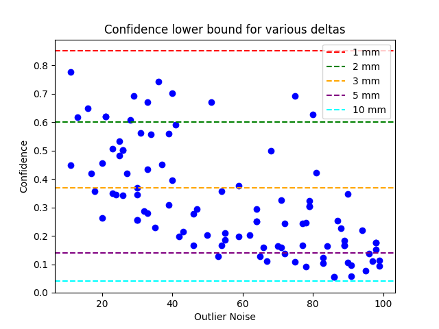
(b)

Figure 8: Confidence based on known poses with additional noise to simulate errors in object poses. (a) Confidence vs outlier noise and ratio. (b) Confidence values for estimated poses (blue points) and confidence thresholds (horizontal lines) based on eq. (12), for various choices of $\delta$.

To assess the ability of the derived confidence score to accurately reflect the quality of the pose we projected a set of 3D points from the object on the image for a known ground truth pose and thereafter, injected noise, $\epsilon$, into these image points according to a Gaussian mixture,

$$p(\epsilon)=p(\epsilon|o)\pi_{o}+p(\epsilon|\overline{o})(1-\pi_{o})$$ (13)

where $\pi_{o}$ is the outlier probability and $p(\epsilon|o)\sim\mathcal{N}(0,\sigma_{o})$, $p(\epsilon|\overline{o})\sim\mathcal{N}(0,\sigma_{\overline{o}})$ are the likelihood of noise for outliers and inliers respectively, with $\sigma_{o}\leq 2\;\;\text{pixels}$ and $\sigma_{o}>10\;\;\text{pixels}$. For these experiments, Fig. 8(a) illustrates the relationship between confidence and noise whereas Fig. 8(b) illustrates how the choice of $\delta$ affects the confidence threshold and the acceptance of the estimated poses. A different depiction of the same trends is achieved with Fig. 9, where confidence drops with the declining accuracy of the back-projected 3D points.

As part of our experimentation, we employed the confidence score in order to admit or reject poses estimated for objects captured in single images. We established a threshold based on eq. (12) for a choice of $\delta=2\;mm$. Fig. 10 illustrates accepted (green) and rejected (red) poses by superimposing the object model on the image based on the estimated pose.

(a) C: 0.79

(b) C: 0.60

(c) C: 0.35

(d) C: 0.16

(e) C: 0.08

Figure 9: Confidence values for increasing (left-to-right) outlier ratio and noise. Top row shows ground truth (gray) vs estimated (orange) pose. Bottom row, back-projections of the noisy 2D points (blue) and the ground truth pose (gray).

Figure 10: Confidence used to accept (green) or reject (red) pose estimates from industrial images with a threshold of 0.6 (via eq. (12) for $\delta=2mm$).

6 Conclusion & Future Work

This paper puts forward a novel score for the quality of pose estimates of objects captured in images, based on geometric consistency with template shape. We also propose a method to build this template using Gaussian processes. Our results demonstrate that the representation is sufficiently accurate to facilitate the computation of a reliable confidence score that reflects the true quality of the estimated pose. In future work, we aim at endowing the shape representation algorithm with theoretical guarantees for full coverage of the object surface irrespective of shape complexity via learned mixtures models and fully automating the choice of reference points.

Appendix 0.A Lower bound for average confidence

Consider the formula for confidence as the average likelihood of distance from reference points,

$$\mathcal{C}(\boldsymbol{T};o)=\sum_{i=1}^{N}w_{i}\left(\underset{k\in\left\{1,\dots,K\right\}}{\max}\hat{q}\left(\boldsymbol{P}_{i}|\boldsymbol{C}_{k};o\right)\right),$$ (14)

For brevity, let $q^{\star}_{i}\sim\mathcal{N}(\mu_{i}^{\star},{\sigma^{\star}}^{2}_{i})\coloneq\underset{k\in\left\{1,\dots,K\right\}}{\max}\hat{q}\left(\boldsymbol{P}_{i}|\boldsymbol{C}_{k};o\right)$ . Also, let $e_{i}=\|\boldsymbol{P}_{i}-\boldsymbol{C}_{i}^{\star}\|$ be the random variable of the difference between the GP prediction $\mu_{i}^{\star}$ and the actual distance of the query point from the reference point $\boldsymbol{C}_{i}^{\star}$ along the direction of the query point, $\boldsymbol{P}_{i}$. Then, the density of $e_{i}$ will be $q^{\star}$ translated at the origin. We now wish to find the average confidence value for $|e_{i}|<\delta$. We therefore integrate eq. (14) from $-\delta$ to $\delta$ over $e_{i}$, i.e.,

$$\overline{\mathcal{C}}=\frac{1}{2\delta}\int_{-\delta}^{\delta}\sum_{i=1}^{N}w_{i}\,q^{\star}_{i}\left(\boldsymbol{P}_{i}|\boldsymbol{C}_{i}^{\star};o\right)\;de_{i}=\frac{1}{2\delta}\sum_{i=1}^{N}w_{i}\int_{-\delta}^{\delta}q^{\star}_{i}\left(\boldsymbol{P}_{i}|\boldsymbol{C}_{i}^{\star};o\right)\;de_{i}$$ (15)

We now consider the expression for the density $q^{\star}_{i}$,

$$q^{\star}_{i}\left(\boldsymbol{P}_{i}|\boldsymbol{C}_{i}^{\star};o\right)=\frac{1}{\sqrt{2\pi}\sigma^{\star}_{i}}\exp\left(-\frac{e_{i}^{2}}{2{\sigma^{\star}}^{2}_{i}}\right)$$ (16)

Since we require that $|e_{i}|<\delta$, it follows that,

$$1>\text{sgn}(e_{i})\cdot\frac{e_{i}}{\delta}$$ (17)

combining the inequalities in eq. (17) with eq. (16), we get,

$$\exp\left(-\frac{e_{i}^{2}}{2{\sigma^{\star}}^{2}_{i}}\right)\geq\text{sgn}(e_{i})\cdot\frac{e_{i}}{\delta}\exp\left(-\frac{e_{i}^{2}}{2{\sigma^{\star}}^{2}_{i}}\right)$$ (18)

Using eq. (18) with eq. (15), we obtain a lower bound of the integral,

$$\begin{split}&\overline{\mathcal{C}}\geq\frac{1}{2\sqrt{2\pi}\delta}\sum_{i=1}^{N}w_{i}\sigma^{\star}_{i}\left(\int_{-\delta}^{0}\frac{e_{i}}{{\sigma^{\star}}^{2}_{i}}\exp\left(-\frac{e_{i}^{2}}{2{\sigma^{\star}}^{2}_{i}}\right)\;de_{i}-\int_{0}^{\delta}\frac{e_{i}}{{\sigma^{\star}}^{2}_{i}}\exp\left(-\frac{e_{i}^{2}}{2{\sigma^{\star}}^{2}_{i}}\right)\;de_{i}\right)\\ &\iff\overline{\mathcal{C}}\geq\frac{1}{\sqrt{2\pi}\delta}\sum_{i=1}^{N}w_{i}\sigma^{\star}_{i}\int_{\delta}^{0}\frac{e_{i}}{{\sigma^{\star}}^{2}_{i}}\exp\left(-\frac{e_{i}^{2}}{2{\sigma^{\star}}^{2}_{i}}\right)\;de_{i}\end{split}$$ (19)

Computing analytically the integral in eq. (19) yields,

$$\overline{\mathcal{C}}\geq\frac{1}{\sqrt{2\pi}\delta^{2}}\sum_{i=1}^{N}w_{i}\sigma_{i}^{\star}\left(1-\exp\left(-\frac{\delta^{2}}{2{{\sigma}^{\star}}^{2}_{i}}\right)\right)$$ (20)

Appendix 0.B Code

Related code available at https://github.com/pansap99/COBRA

References

- [1] Achlioptas, P., Diamanti, O., Mitliagkas, I., Guibas, L.: Learning representations and generative models for 3d point clouds (2017), http://arxiv.org/abs/1707.02392
- [2] Blum, H., Sarlin, P.E., Nieto, J., Siegwart, R., Cadena, C.: The Fishyscapes Benchmark: Measuring Blind Spots in Semantic Segmentation. Intl. Journal of Computer Vision 129(11), 3119–3135 (2021). https://doi.org/10.1007/s11263-021-01511-6
- [3] Brock, A., Lim, T., Millar, R., Nicholas, W.: Generative and discriminative voxel modeling with convolutional neural networks. In: NeurIPS 3D Deep Learning Workshop. pp. 1–9 (2016)
- [4] Chen, Z., Zhang, H.: Learning implicit fields for generative shape modeling. In: 2019 IEEE/CVF Conf. on Computer Vision and Pattern Recognition (CVPR). pp. 5932–5941 (2019). https://doi.org/10.1109/CVPR.2019.00609
- [5] Chibane, J., Alldieck, T., Pons-Moll, G.: Implicit functions in feature space for 3d shape reconstruction and completion. 2020 IEEE/CVF Conf. on Computer Vision and Pattern Recognition (CVPR) pp. 6968–6979 (2020)
- [6] Do, C.B., Batzoglou, S.: What is the expectation maximization algorithm? Nature biotechnology 26(8), 897–899 (2008)
- [7] Dragiev, S., Toussaint, M., Gienger, M.: Gaussian process implicit surfaces for shape estimation and grasping. In: 2011 IEEE Intl. Conf. on Robotics and Automation. pp. 2845–2850 (2011). https://doi.org/10.1109/ICRA.2011.5980395
- [8] Farshian, A., Götz, M., Cavallaro, G., Debus, C., Nießner, M., Benediktsson, J.A., Streit, A.: Deep-learning-based 3-d surface reconstruction—a survey. Proc. of the IEEE 111(11), 1464–1501 (2023). https://doi.org/10.1109/JPROC.2023.3321433
- [9] Genova, K., Cole, F., Sud, A., Sarna, A., Funkhouser, T.A.: Local deep implicit functions for 3d shape. 2020 IEEE/CVF Conf. on Computer Vision and Pattern Recognition (CVPR) pp. 4856–4865 (2019)
- [10] Hodan, T., Barath, D., Matas, J.: Epos: Estimating 6d pose of objects with symmetries. In: Proc. of the IEEE/CVF Conf. on computer vision and pattern recognition. pp. 11703–11712 (2020)
- [11] Hodaň, T., Matas, J., Obdržálek, Š.: On evaluation of 6d object pose estimation. In: Hua, G., Jégou, H. (eds.) Computer Vision – ECCV 2016 Workshops. pp. 606–619. Springer Intl. Publishing, Cham (2016)
- [12] Jayasumana, S., Hartley, R., Salzmann, M., Li, H., Harandi, M.: Kernel methods on riemannian manifolds with gaussian rbf kernels. IEEE Transactions on Pattern Analysis and Machine Intelligence 37(12), 2464–2477 (2015). https://doi.org/10.1109/TPAMI.2015.2414422
- [13] Kim, S.h., Hwang, Y.: A survey on deep learning based methods and datasets for monocular 3D object detection. Electronics 10(4), 517 (2021)
- [14] Lakshminarayanan, B., Pritzel, A., Blundell, C.: Simple and scalable predictive uncertainty estimation using deep ensembles. In: Proc. of the 31st Intl. Conf. on Neural Information Processing Systems. p. 6405–6416. NIPS’17, Red Hook, NY, USA (2017)
- [15] Liao, Y., Donné, S., Geiger, A.: Deep marching cubes: Learning explicit surface representations. In: 2018 IEEE/CVF Conf. on Computer Vision and Pattern Recognition. pp. 2916–2925 (2018). https://doi.org/10.1109/CVPR.2018.00308
- [16] Lin, J., Wei, Z., Ding, C., Jia, K.: Category-level 6d object pose and size estimation using self-supervised deep prior deformation networks. In: Computer Vision – ECCV 2022. pp. 19–34. Springer Nature Switzerland, Cham (2022)
- [17] Lin, J., Wei, Z., Li, Z., Xu, S., Jia, K., Li, Y.: Dualposenet: Category-level 6d object pose and size estimation using dual pose network with refined learning of pose consistency. In: 2021 IEEE/CVF Intl. Conf. on Computer Vision (ICCV). pp. 3540–3549 (2021). https://doi.org/10.1109/ICCV48922.2021.00354
- [18] Liu, F., Liu, X.: Learning implicit functions for dense 3d shape correspondence of generic objects. IEEE Trans. Pattern Anal. Mach. Intell. 46(3), 1852–1867 (2023). https://doi.org/10.1109/TPAMI.2022.3233431
- [19] Lloyd, S.: Least squares quantization in pcm. IEEE transactions on information theory 28(2), 129–137 (1982)
- [20] Loquercio, A., Segu, M., Scaramuzza, D.: A general framework for uncertainty estimation in deep learning. IEEE Robotics and Automation Letters 5(2), 3153–3160 (2020). https://doi.org/10.1109/LRA.2020.2974682
- [21] Mescheder, L., Oechsle, M., Niemeyer, M., Nowozin, S., Geiger, A.: Occupancy networks: Learning 3d reconstruction in function space. In: 2019 IEEE/CVF Conf. on Computer Vision and Pattern Recognition (CVPR). pp. 4455–4465 (2019). https://doi.org/10.1109/CVPR.2019.00459
- [22] Mildenhall, B., Srinivasan, P.P., Tancik, M., Barron, J.T., Ramamoorthi, R., Ng, R.: Nerf: representing scenes as neural radiance fields for view synthesis. Commun. ACM 65(1), 99–106 (dec 2021). https://doi.org/10.1145/3503250, https://doi.org/10.1145/3503250
- [23] Nguyen, V.N., Groueix, T., Hu, Y., Salzmann, M., Lepetit, V.: Nope: Novel object pose estimation from a single image. arXiv preprint arXiv:2303.13612 (2023)
- [24] Niemeyer, M., Mescheder, L.M., Oechsle, M., Geiger, A.: Occupancy flow: 4d reconstruction by learning particle dynamics. 2019 IEEE/CVF Intl. Conf. on Computer Vision (ICCV) pp. 5378–5388 (2019)
- [25] Park, J.J., Florence, P., Straub, J., Newcombe, R., Lovegrove, S.: Deepsdf: Learning continuous signed distance functions for shape representation. In: Proc. of the IEEE/CVF Conf. on computer vision and pattern recognition. pp. 165–174 (2019)
- [26] Paschalidou, D., Gool, L.V., Geiger, A.: Learning unsupervised hierarchical part decomposition of 3d objects from a single rgb image. 2020 IEEE/CVF Conf. on Computer Vision and Pattern Recognition (CVPR) pp. 1057–1067 (2020)
- [27] Qi, C., Su, H., Mo, K., Guibas, L.: Pointnet: Deep learning on point sets for 3d classification and segmentation. In: 2017 IEEE Conf. on Computer Vision and Pattern Recognition (CVPR). pp. 77–85 (2017). https://doi.org/10.1109/CVPR.2017.16
- [28] Rambach, J., Deng, C., Pagani, A., Stricker, D.: Learning 6dof object poses from synthetic single channel images. In: 2018 IEEE Intl. Symposium on Mixed and Augmented Reality Adjunct (ISMAR-Adjunct). pp. 164–169. IEEE (2018)
- [29] Rasmussen, C.E.: Gaussian Processes in Machine Learning, pp. 63–71. Springer Berlin Heidelberg (2004). https://doi.org/10.1007/978-3-540-28650-9_4
- [30] Shawe-Taylor, J., Cristianini, N.: Kernel Methods for Pattern Analysis. Cambridge University Press (2004)
- [31] Shi, G., Zhu, Y., Tremblay, J., Birchfield, S., Ramos, F., Anandkumar, A., Zhu, Y.: Fast uncertainty quantification for deep object pose estimation. In: 2021 IEEE Intl. Conf. on Robotics and Automation (ICRA). p. 5200–5207 (2021). https://doi.org/10.1109/ICRA48506.2021.9561483
- [32] Sundermeyer, M., Hodaň, T., Labbé, Y., Wang, G., Brachmann, E., Drost, B., Rother, C., Matas, J.: Bop challenge 2022 on detection, segmentation and pose estimation of specific rigid objects. In: 2023 IEEE/CVF Conf. on Computer Vision and Pattern Recognition Workshops (CVPRW). pp. 2785–2794 (2023). https://doi.org/10.1109/CVPRW59228.2023.00279
- [33] Tremblay, J., To, T., Sundaralingam, B., Xiang, Y., Fox, D., Birchfield, S.: Deep object pose estimation for semantic robotic grasping of household objects. In: Billard, A., Dragan, A., Peters, J., Morimoto, J. (eds.) Proc. of The 2nd Conf. on Robot Learning. Proc. of Machine Learning Research, vol. 87, pp. 306–316 (29–31 Oct 2018)
- [34] Wang, H., Sridhar, S., Huang, J., Valentin, J., Song, S., Guibas, L.J.: Normalized object coordinate space for category-level 6d object pose and size estimation. In: 2019 IEEE/CVF Conf. on Computer Vision and Pattern Recognition (CVPR). pp. 2637–2646 (2019). https://doi.org/10.1109/CVPR.2019.00275
- [35] Wang, N., Zhang, Y., Li, Z., Fu, Y., Liu, W., Jiang, Y.G.: Pixel2mesh: Generating 3d mesh models from single rgb images. In: Proc. European Conf. Computer Vision – ECCV 2018. p. 55–71 (2018). https://doi.org/10.1007/978-3-030-01252-6_4
- [36] Zheng, Z., Yu, T., Dai, Q., Liu, Y.: Deep implicit templates for 3d shape representation. In: Proc. of the IEEE/CVF Conf. on Computer Vision and Pattern Recognition. pp. 1429–1439 (2021)
- [37] Zhu, Y., Li, M., Yao, W., Chen, C.: A review of 6d object pose estimation. In: 2022 IEEE 10th Joint Intl. Information Technology and Artificial Intelligence Conf. (ITAIC). vol. 10, pp. 1647–1655 (2022). https://doi.org/10.1109/ITAIC54216.2022.9836663