Topological properties of finite-size heterostructures of magnetic topological insulators and superconductors
Abstract
Heterostructures of magnetic topological insulators (MTIs) and superconductors (SCs) in two-dimensional (2D) slab and one-dimensional (1D) nanoribbon geometries have been predicted to host, respectively, chiral Majorana edge states (CMESs) and Majorana bound states (MBSs). We study the topological properties of such MTI/SC heterostructures upon variation of the geometry from wide slabs to quasi-1D nanoribbon systems and as a function of the chemical potential, the magnetic doping, and the induced superconducting pairing potential. To do so, we construct effective symmetry-constrained low-energy Hamiltonians accounting for the real-space confinement. For a nanoribbon geometry with finite width and length, we observe different phases characterized by CMESs, MBSs, as well as coexisting CMESs and MBSs, as the chemical potential, the magnetic doping and/or the width are varied.
I Introduction
Topological superconductors are fascinating phases of matter which have stirred significant interest in the scientific community [1, 2, 3]. These phases display gapped bulk states with superconducting pairing as well as topologically protected gapless surface states, which have been predicted to be Majorana states. The search for these quasi-particles has stimulated an intense research activity, primarily owing to their potential for quantum computing [4, 5]. Nevertheless, proposed realizations of topological superconductors with large enough bulk gaps remain rare and Majorana states remain elusive and controversial.
Bringing together superconducting pairing and spin-orbit (SO) or SO-like interactions is a promising avenue for creating topological superconductivity. It has for instance been studied in superconductors with strong SO interactions [6, 7, 8], in topological materials where doping with Nb, Sr or Cu yields a superconducting gap in the bulk [9, 10], or in heterostructures combining strong SO interactions or SO-like interactions induced by a magnetic texture with a conventional superconductor [11, 12, 13, 14, 15, 16, 17, 18, 19, 20, 21]. Breaking time-reversal symmetry (TRS) is also often necessary for the emergence of low-dimensional surface states such as chiral edge states or bound states.
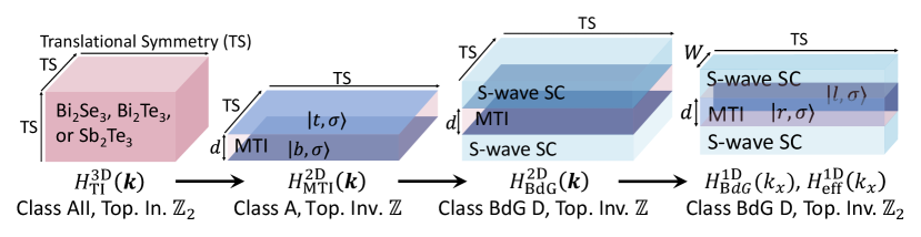
TRS can also be broken by an external magnetic field, but this may not be compatible with superconductivity. It is thus desirable to explore intrinsic magnetism (e.g. via magnetic doping) of heterostructures as an alternative [22, 23, 24, 25]. In our work, we study MTI/SC heterostructures where the interplay between superconducting pairing, spin-orbit coupling, and TRS breaking leads to the appearance of topological superconducting phases. Our study will apply to heterostructures consisting of -wave SCs and magnetically doped compounds of the Bi2Se3 family. The effective realization of such heterostructures has recently shown promising progress [22, 23]. We will consider thin MTI films, which have become experimentally realizable over the past decade [26, 27, 28]. A comprehensive description of MTI thin films is achieved by the construction of a symmetry-constrained Hamiltonian [29, 2]. Here, we introduce this model as a basis for the subsequent finite-size calculations and to relate our study to concrete material systems. We discuss its applicability for the system we investigate and we comment on the limits of such a model [30, 31, 32].
In recent works, planar translation-invariant geometries and confined quasi-1D geometries of MTI/SC heterostructures have been suggested as a potential platform for Majorana physics. Such systems have been studied for specific values of the chemical potential , of the strength of the magnetic exchange interaction with the magnetic dopants, and for specific sizes [33, 18, 21]. Here, we provide a more comprehensive treatment, studying a wider region of the phase diagram in space and the nature of the topological states when the in-plane size of the heterostructure is varied from infinitely large to finite. Moreover, we discuss the transition from chiral Majorana edge states (CMES) to Majorana bound states (MBS) and their respective localization. In the following, we will refer to planar translation-invariant geometries as “slab geometries” and to in-plane confined geometries as “nanoribbons”. For nanoribbons with intermediate width, and depending on the magnitude of the magnetic exchange term in the MTI, we observe regions in the phase diagram where the low-energy sector hosts coexisting CMESs and MBSs. Our understanding of the topological properties associated with these finite-size systems, from two-dimensional to quasi-one-dimensional, is based on symmetry-constrained analytical low-energy models that we construct throughout this paper. These characterize the appearance of gapless surface (edge or end) states through the bulk-edge correspondence.
This paper is organized as follows: In Sec. II, we introduce the effective models we use for the description of the MTI. First, we review the construction of a symmetry-constrained Hamiltonian which characterizes a 3-dimensional (3D) topological insulator (TI). Then we construct effective models for a thin MTI slab system and for a nanoribbon geometry by considering the low-energy states arising from quantum confinement in the 3D model. We study the occurence of chiral edge modes as a function of the magnetic exchange term and as a function of the width of the nanoribbon. In Sec. III, we study the topological properties of an MTI/SC slab and then we investigate the occurrence of CMES and MBS in MTI/SC with nanoribbon geometries.
II Effective model for the MTI
II.1 Symmetry-constrained Hamiltonian
A convenient way of describing the topological properties of a (3D) compound of the family is via the following Hamiltonian [34, 35, 29, 2],
| (1) | ||||
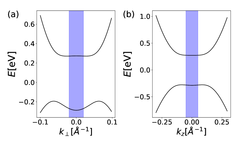
where , , and , , , , , , , , are real coefficients. This Hamiltonian acts in the (atomic) low-energy basis of states through the Pauli matrices and which act, respectively, in the spin and parity spaces. The parity operation, equivalent to inversion symmetry in 3D, acts on according to the matrix representation and flips the momentum vector, leaving the Hamiltonian invariant: . This Hamiltonian is valid in the vicinity of the point, where it describes the low-energy properties of the system. In Fig. 2, we show the eigenenergies of this Hamiltonian.
This Hamiltonian relies on a long-wavelength approximation and is a priori valid only for finite systems above a certain size. The coefficients appearing in the Hamiltonian can be determined by fitting the energy spectrum to experimental data or extracting the parameters from ab-initio calculations (see Ref. [2]). The distance from the point up to which this model Hamiltonian is a good approximation allows an estimate of the possible size of the system. The band structure of the Hamiltonian (1) is in good agreement with ab-initio calculations for , , and [36]. This implies that the system thickness in the direction should be larger than Å while the width and the length , respectively, in the direction and -directions should be larger than Å.
It is also important to note that is constrained by the symmetries of the system, specifically TRS, inversion symmetry, and the three-fold rotation symmetry around the axis. The atomic states used to construct the Hamiltonian are based on quintuple layer unit cells which respect the aforementioned symmetries [2]. For the materials we consider, the thickness (along the direction) of a quintuple layer is approximately nm. In the following, we will consider systems with widths and lengths larger than nm, which is much larger than the length of a unit cell in the and -directions (below nm). This allows us to study a continuum of lengths above nm along these directions. We notice that nm or nm is a reasonable lower limit of what is currently achieved experimentally. We will consider slabs and nanoribbons of family compounds consisting of two or more quintuple layers (thickness larger than Å).
II.2 Slab geometry
Let us consider a TI slab (a planar translation-invariant geometry) with a finite thickness along the direction, with bottom and top surfaces of the slab located, respectively, at and . We replace , impose vanishing wave functions as boundary conditions at and , and denote by and the two lowest eigenenergies of , each of which is twofold degenerate because of TRS. Magnetic doping can be accounted for by adding a TRS-breaking Zeeman term ; the system is now an MTI. The respective eigenstates of the Hamiltonian will be denoted by and , where . Projecting on the basis gives rise to a Hamiltonian which describes an MTI slab [38, 39] (we use in the following),
| (2) | ||||
where the coefficients are given by
| (3) |
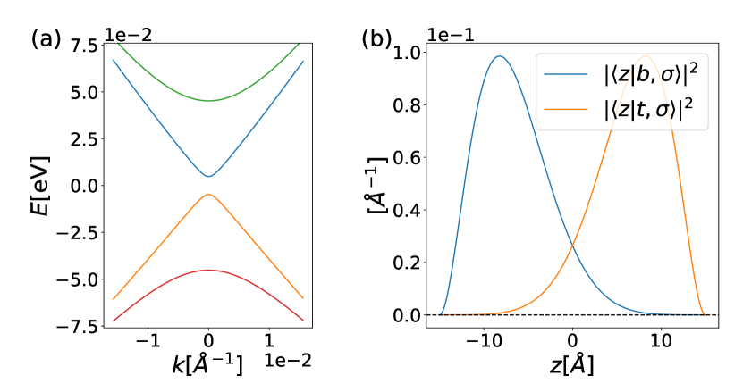
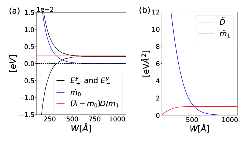
In Table 1 we list the values of the coefficients , , and for several values of the thickness, starting from two quintuple layers, and calculated from Eq. (II.2), using the parameters of the 3D Hamiltonian (1) for bulk Bi2Se3 [29]. A diagonalization of yields four energy bands with a finite gap at the point. This is shown in Fig. 3(a) where, for simplicity, we considered the chemical potential of the system to be tuned to .
| d[Å] | [eV] | [eV | [eV | [eV |
|---|---|---|---|---|
| 4.09 | ||||
| 4.06 | ||||
| 4.06 | ||||
| 4.06 | ||||
| 4.06 | ||||
| 4.06 |
The eigenstates and allow the construction of states and localized near the top and bottom surfaces, respectively. These are indeed given by and and have localization lengths Å (see Fig. 3(b)). In this basis of states, the Hamiltonian reads
| (4) | ||||
where and the Pauli matrices and act, respectively, on the top/bottom ( degree of freedom and the spin degree of freedom. Eq. (4) is the starting point of Sec. III, where we study an MTI/SC heterostructure.
In case of magnetic doping (), the symmetry class of the Hamiltonian is denoted A (unitary symmetry class) and the topological phase is characterized by an integer Chern number [40]. In contrast, at , the Hamiltonian has TRS and fits in the symmetry class AII (symplectic symmetry class) where the topological sector is characterized by a topological invariant.
Determining the value of the topological invariant requires not only the low-energy eigenstates but also information at large momenta. However, determining the difference between the topological invariants characterizing two phases separated by the closing of the gap is possible: in this case, we only need the eigenstates around the point, where the gap closes, which we determine from the Hamiltonian in Eq. (2). These eigenstates and thus the topological invariants do not depend on or since those enter the Hamiltonian with an identity matrix. Hence, let us consider the case .
The low-energy model can predict the occurrence of topological phase transitions via a sign change of the effective gap . At , the sign change of the gap , when increasing the thickness from 2 to 3 quintuple layers, shows a transition between a trivial insulating and a quantum spin Hall insulating phase (see Table 1). At , the Chern number vanishes, indicating a trivial phase. In contrast, a sufficiently large magnetic exchange term yields a quantum anomalous Hall (QAH) phase, independently of the sign and magnitude of , as was also observed in Ref. [41].
Whether or not the materials we consider indeed display a quantum spin Hall phase (without doping) below 6 quintuple layers is still under debate in the literature. For instance, for Bi2Se3 it has been argued that the Coulomb interaction leads to a significant hybridization of the surface states, which could open a trivial gap below 6 quintuple layers [42, 32]. GW computations performed for Bi2Se3 also concluded that the gap below 6 quintuple layers is trivial, but a gap inversion remains for Bi2Te3 [30]. Our following study will apply to a thin slab in (or near) the QAH regime, which is attainable independently of the sign of for a large enough magnetic exchange magnitude . Experimental studies on such systems have already been performed, and the QAH phase has been characterized, e.g., in Cr- and V-doped (Bi,Sb)2Te3 [43].
II.3 One-dimensional model for an MTI nanoribbon
Next, we consider a 2D nanoribbon geometry with a finite width along the direction with left and right edges of the slab respectively located at and . Moreover, we assume which would correspond to the QAH regime for . The goal of this section is to estimate the critical width above which the nanoribbon effectively enters a QAH phase, manifested in one chiral state at each edge of the slab. Below this width, the hybridization of edge states on opposite edges becomes significant.
The Hamiltonian (2) describes the 2D MTI slab and consists of the two independent blocks and . For the description of the nanoribbon, we substitute and we impose vanishing wave functions at the edges of the slab. In the following, we assume without loss of generality, since the case would only exchange the roles of and . The block has an inverted mass gap , which results in a pair of edge states arising from the quantum confinement along the direction. The associated energies at converge to when or is increased as shown respectively in Fig. 4(a) or Fig. 4(b) (red line). In contrast, has a normal mass gap , so for the parameter regime we consider its low-energy states arising from the quantum confinement are topological trivial. They have energies greater than or smaller than , respectively, as shown in Fig. 4.
For non-vanishing , the energies of both topological edge states are shifted compared to the energies of the bulk states. As a consequence, for large enough , i.e., , the low-energy states at the point are outside the energy gap. As we would like to build a simple ribbon model, we will consider small values of in the following, such that the low-energy states at the point are in the gap. Hence, in Fig. 4 we have assumed . For a description of the effects of larger values of , we refer to Ref. [44].
At , where the Fermi energy corresponds to the red line in Fig. 4, we can construct a Hamiltonian which describes the edge states around the Fermi level by only considering the block , as it describes the relevant low-energy physics. Substituting and imposing vanishing wave functions at the edges of the slab, becomes,
| (5) | ||||
Let us denote the lowest eigenergies at by and , and the associated eigenstates by and . Similarly to the previous section, we project on the low-energy eigenstates of and thus obtain an effective 1D Hamiltonian describing the slab with finite width at low energies (see App. A)
| (6) |
where are Pauli matrices acting in the basis and the parameters are given by
| (7) |
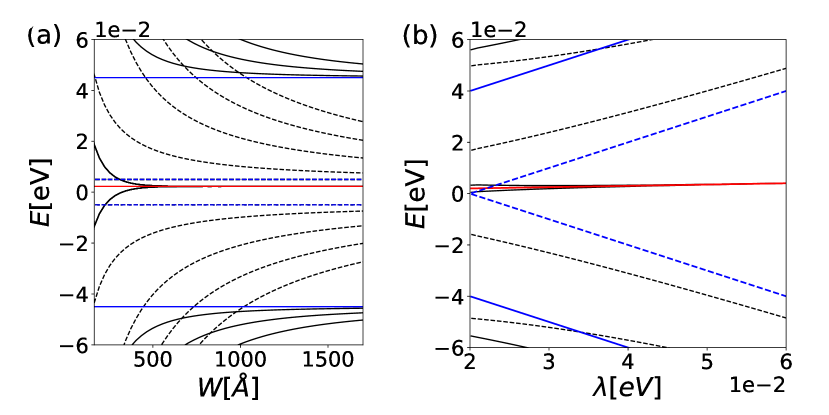
The coefficients and are plotted as functions of the width in Fig. 5. The coefficient varies only very weakly: for the parameters considered in Fig. 5, and it has a maximum variation over the range of investigated.
Next, we introduce the states and which are localized on the left and right edges of the ribbon, respectively. The parameter represents the overlap between both edge states, so it determines the topological phase of the slab. For small overlap, in the QAH phase, one chiral state appears at each edge. For large , the overlap of these edge states brings the system into a topologically trivial phase. In this 1D limit, a symmetry-class A Hamiltonian has indeed trivial topological properties [40].
From Fig. 5, we see that for Å, cannot be neglected compared to the other terms in the Hamiltonian, so the 1D system becomes topologically trivial. For Å, on the other hand, is negligible, so the slab enters a QAH phase.
III MTI/SC heterostructures
III.1 Surface states of the MTI and proximity effect
We now consider the superconducting proximity effect [45, 18] originating from the contact with -wave superconductors on the top and bottom surfaces of the MTI slab. We assume that they give rise to the pairing potentials and , respectively, with two real parameters and . This is described by extending the Hamiltonian (4) to the Nambu basis,
| (8) | ||||
where the Pauli matrices act in the particle-hole space. Expressed in this form, it is straightforward to check that the Hamiltonian has particle-hole symmetry and at it also has TRS , where , , and is the complex conjugation operator.
III.2 Topological properties for the slab geometry
For a slab geometry, the topological phase transitions are signaled by the change of the 2D bulk invariant of the model (8) and happen at the gap closing points. For the special case , and the Hamiltonian can be simplified to (see App. B)
| (9) | ||||
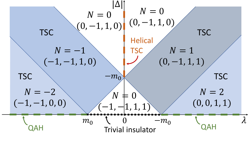
with and , and . It is then straightforward to calculate the topological invariant [18]. The Hamiltonian is a sum of independent massive Dirac Hamiltonians, so the topological invariant is the sum of the winding numbers associated with each of the independent Hamiltonians . At fixed , the cases and both result in the same phase diagram for , even though the decompositions in terms of are different. In Fig. 6, we show this phase diagram along with the details of the decomposition in terms of for and .
Building on this, we can extend the phase diagram for , and by considering the phase boundaries. As topological phase transitions happen only at the gap closing points, we find that they are described by the equation
| (10) | ||||
with . This result generalizes the study performed in Ref. [18] where an equation for the phase boundaries was given for . The term, being proportional to and involving only terms of second order in the momentum, does not influence the phase boundaries.
III.3 Ribbon geometry for ,
Next we investigate the effect of in-plane confinement on the topological properties of the MTI/SC heterostructure for the case where and . We show that for a confined geometry, the topological properties depend on the decomposition of in terms of , and on the mass values . This is in contrast to the translation-invariant geometry, where alone determines the topological properties at .
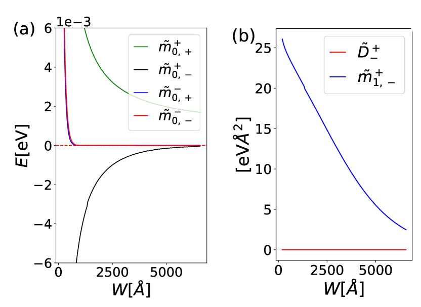
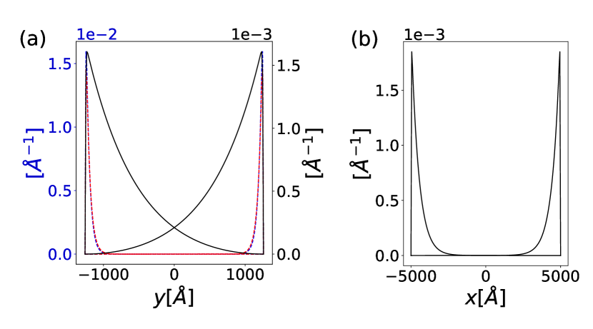
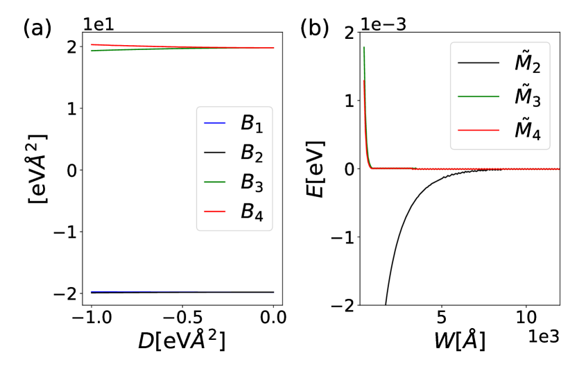
First, we consider a ribbon geometry with width along the direction. The calculation performed in Sec. II.3 can be easily adapted since the Hamiltonian (9) is a sum of independent massive Dirac Hamiltonians. For each term where the mass and the parameter correspond to the inverted regime, i.e., , a pair of low-energy states appears, which we denote by and and which have the respective energies and . These energies are plotted in Fig. 7 as a function of the width of the ribbon. Figure 8(a) shows the localization of and along the direction in an MTI/SC nanoribbon with width Å. One finds that decreases when increases and that the overlap between and is proportional to (see Fig. 8(a) and Fig. 7(a)).
For large regions of the phase diagram the masses can differ significantly. At intermediate widths , this causes the coexistence of chiral low-energy states strongly localized at the edges with states which overlap along the direction [46]. For instance, in Fig. 7, for Å, (blue line) and (red line) are small, so we expect that , , , and are edge states. In contrast, (black line) is larger so the states , and overlap along . The states overlaping along the direction are then described by a 1D bulk Hamiltonian, with parameters and which depends on .
Next, we also consider confinement along the direction such that the length in the direction satisfies . In this case, we find that the overlapping states and give rise to new low-energy states and which are localized at both ends of the ribbon if (see Fig. 8(b)). These states are Majorana bound states (MBS), which arise from the confinement of a 1D BdG D Hamiltonian with topologically non-trivial number.
We are interested only in states with negligible energy, i.e., with energy below a small energy threshold . If , the Hamiltonian has a non-zero BdG D Chern number [18], and if , the states and represent a chiral Majorana edge state (CMES) at each edge of the system. In this description, CMESs with different chiralities can coexist at the same edge if and for several . This description is valid at vanishing disorder in the system. At finite disorder, CMESs of opposite chirality will hybridize, resulting in 0, 1 or several copropagating CMESs at each edge. It is worth noting that a pair of copropagating CMESs at each edge is topologically equivalent to a QAH chiral edge state [46]. If , , and , then the states and form a pair of MBS with negligible energy, localized at the end of the nanoribbon. If disorder were included in our description, we would either find 0 or 1 pairs of MBS in the system.
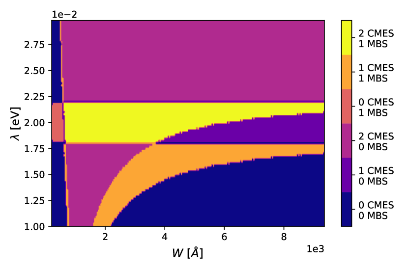
As an example, let us consider a Bi2Se3 nanoribbon with thickness Å (see Table 1) and with , (the Bi2Se3 nanoribbon is a quantum spin hall insulator at and ). We consider the regime where , which corresponds to the experimentally relevant range of superconducting pairings. We arbitrarily set to be one tenth of the superconducting pairing magnitude . In Fig. 9, we display the number of CMES and the number of MBS appearing below , as a function of and .
In the limit , the number of CMES is in agreement with the phase diagram of Fig. 6. Moreover, for the region of Fig. 6 where , and when is small enough such that there is no edge states in the direction, the system simply hosts a pair of Majorana bound states [21]. For intermediate range of widths, we observe a richer phase diagram. Indeed, at fixed , varying the width up to Å, we cross different phases. Namely, we observe a region characterized by either one CMES or two CMES with the same chirality and MBS.
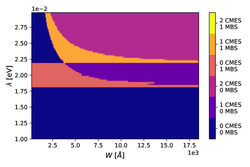
In Fig. 10, we display the number of CMESs and the number of MBSs in the case , (the Bi2Se3 nanoribbon is a trivial insulator at and ). For a straightforward comparison with Fig. 9, we consider with opposite sign and otherwise identical parameters. For wide enough nanoribbons (), we observe either 0, 1 or 2 CMESs in agreement with Fig. 6. Similarly to the results shown in Fig. 9, when is small enough, we observe 0, 1, and 0 end states, respectively, for the regions of Fig. 6 where , , and . The region of intermediate width is qualitatively different from what we observe in Fig. 10. Only in the region of Fig. 6 where , we observe a phase characterized by one CMES and MBS.
III.4 Ribbon geometry for general parameters
In the previous section, the choice of parameters , , and made it possible to calculate the low-energy states for the in-plane confined geometry without further approximations. Here, we discuss the more general parameter regime , , , and .
In the following, we consider meV and we write . Moreover, we restrict our study to the case , and where are the two highest energies associated to the Hamiltonian (8) for the specific MTI thickness Å. For this regime of parameters, we assume that each pair of energy bands around the point (see Eq. (8)) can be described to a good approximation by a massive Dirac Hamiltonian. Therefore, close enough to the point, we express in Eq. (8) by where
| (11) |
where the Pauli matrices act in a transformed basis of states which coincides with the low-energy states of at . The parameters , , and are obtained by fitting the resulting energies around the point with the corresponding energy band of . We further impose that the effective parameters should reduce to and at , , and that they evolve adiabatically in parameter space at constant topological invariant , which is determined by the phase boundaries evolution according to Eq. (10).
For sufficiently small width and , the low-energy edge states associated to hybridize. Similarly to Sec. II.3, a 1D Hamiltonian can be derived from ,
| (12) |
where and are Pauli matrices acting in the basis where and are the eigenstates of with the two lowest eigenenergies . The coefficients appearing in the previous equation are given by , , .
III.4.1
First, we consider (such that as we already consider in Sec. II.3), and . This case is simplified by the facts that (i) the parameter appears in the Hamiltonian with a matrix, in contrast to the term proportional to , and (ii) the parameter multiplies a factor . Therefore the term does not change the value of the masses and has an important effect only if . Since here we consider at most eV, for has no strong qualitative effect on the low-energy states at the system widths and lengths we consider.
As an illustration in Fig. 11, we show the change of with for a specific value of , and we show how Fig. 7(a) is modified for eV due to the evolution of the low-energy states which appear due to the confinement along when .
III.4.2
At , the phase boundaries are shifted according to Eq. (10). However, for each phase with a fixed topological invariant, we checked from that each pair of bulk bands retains the same topological character. Therefore, no strong qualitative changes happen for the phase diagram, as we show in Fig. 12 for the case .
III.4.3
The case is more subtle because the energies around the point can change significantly. For simplicity, we only consider values for and corresponding to the region with topological phase in the infinite 2D geometry with where are the two highest energies of the Hamiltonian (8). Moreover, we focus on the case , unless otherwise stated. From our study in the previous section, we expect this region to be interesting since at it shows a coexistence of two CMES and one MBS (or 1 CMES at very large ). How do these topological states change for ?
Firstly, both high energies remain similar as in the case , since here . Therefore, above Å, the low-energy states arising from confinement of the bulk states associated to are copropagating CMES with negligible energy, as it is the case for (blue and red lines in Fig. 7(a)). Secondly, we describe the evolution of the low energy bands at by with given in Eq. (11).
For the phase we consider, we know that at the topological low-energy states correspond to only one CMES at each edge. This means that the total number of inverted bulk bands cannot change when changes. Taking this constraint into account, we observe from our fit that the topological characters of the first and second energy bands are exchanged at small with concomitant sign changes of and . Although this has no impact on the phase diagram at , this is important for the topological properties of the low-energy states for nanoribbons of intermediate width .
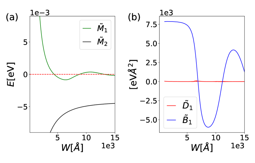
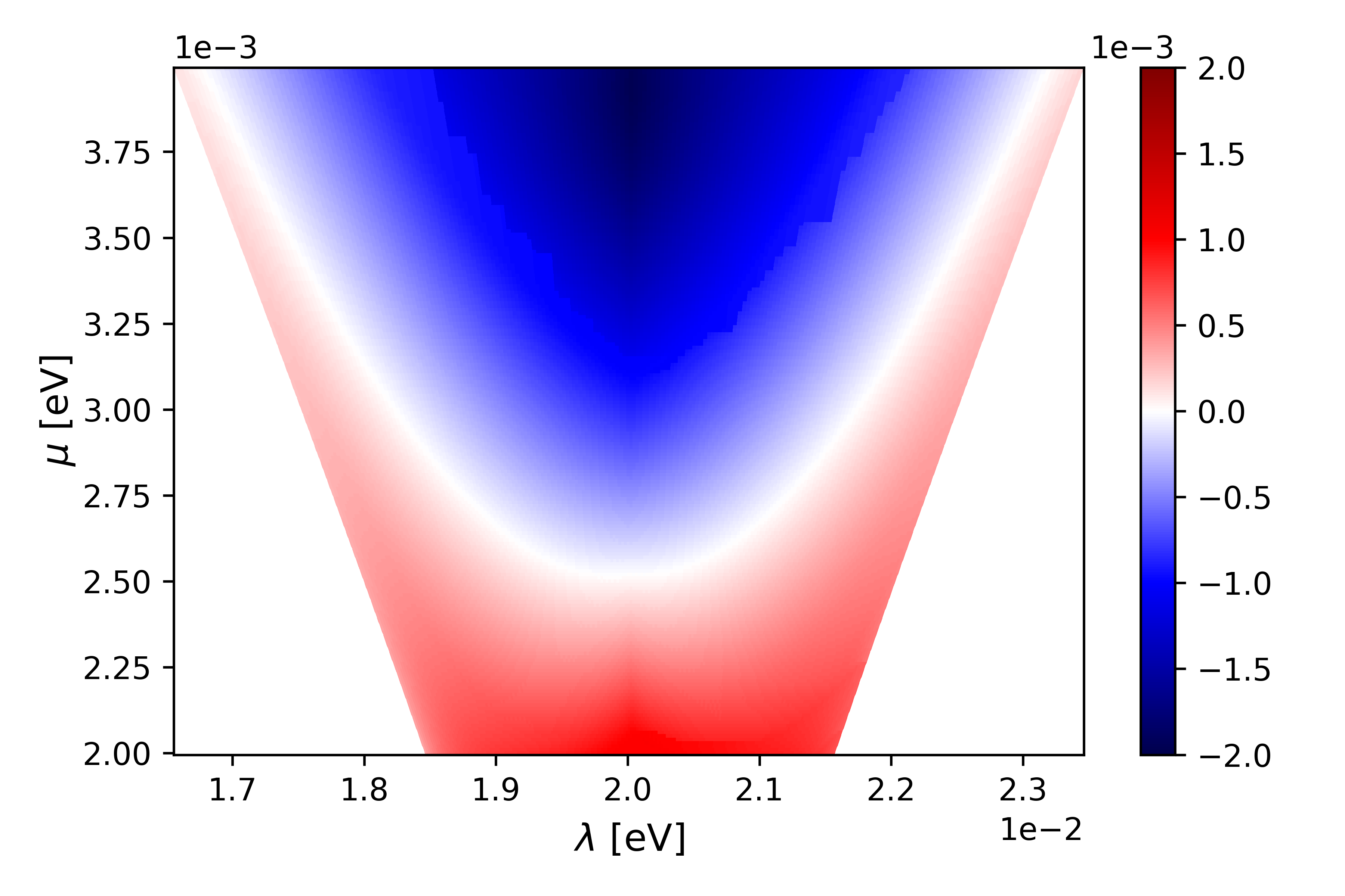
In the example of Fig. 13, we observe that takes non-negligible values for Å, with an oscillating behavior as a function of . This oscillating behavior is also observed as a function of and when the width is fixed, as it is shown in Fig. 14. Moreover, the sign of and the resulting sign of also oscillate as function of , and . For the parameters and considered in Fig. 14, is positive, so the sign changes of are determined by . From our theory, this signals topological transitions as , and are varied.
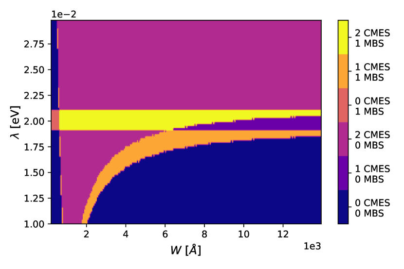
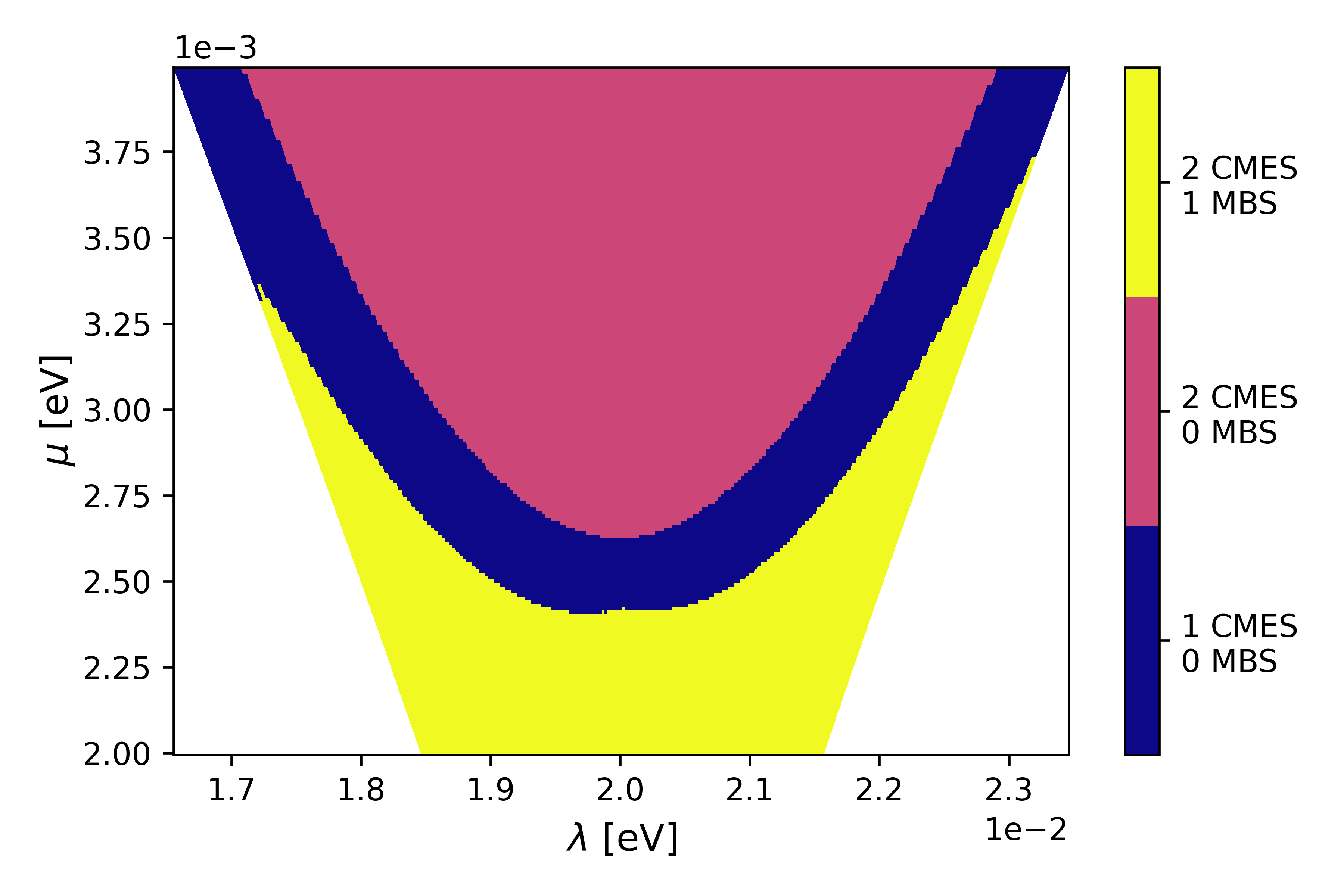
Let us also consider confinement along the direction, such that the length of the nanoribbon satisfies . Here again, for concreteness, we are interested only in states with energy below a certain threshold which we arbitrarily set to be one tenth of the superconducting pairing magnitude . If , the state associated to the energy is a CMES with negligible energy and with chirality opposite to the copropagating states associated to . This description is valid at vanishing disorder in the system. At finite disorder, CMES of opposite chirality hybridize, resulting in only one CMES in the system. If and (see, e.g., the red phase in Fig. 14), then a pair of MBS with negligible energy, localized at the ends of the nanoribbon, appears. In this case, the low-energy states in the system are both copropagating CMES associated with and a pair of MBS. In Fig. 15, we display the number of CMES and the number of MBSs appearing at low energies as a function of and for .
Finally, let us comment the situation in which the nanoribbon is very thin, here meaning , where the states arising from confinement of the bulk states associated to hybridize in the bulk and do not result in topological low-energy states. In this case, and (see Fig. 13), which yields a topological phase with a pair of MBS, localized at the ends of the nanoribbon, and without any CMES, reflecting the scenario proposed in Refs. [21, 33]. Note that this topological phase can arise for both greater and smaller than , hence not requiring the MTI system (with ) to be in the QAH phase for very large widths. While this phase only appears in a narrow window of near , this region is enlarged when is increased, similar to the topological phase with 2 CMES and 1 MBS in Fig. 15.
IV Conclusion
We have studied the topological properties of finite MTI/SC heterostructures using symmetry-constrained low-energy models. We started by developing analytical models for MTI slabs with a finite thickness as well as MTI nanoribbons with finite thickness and width. We investigated the appearance of low-energy states as a function of the magnetic doping, the chemical potential and the system size. Next, we considered such finite geometries subject to superconducting pairing induced by two superconductors at the top and bottom surfaces. For very wide nanoribbons the low-energy states are the chiral edge states as predicted by the 2D bulk topological invariant. For finite width nanoribbons, we constructed and studied low-dimensional models describing the low-energy properties of our system. In a nanoribbon geometry with finite width and length, we observed regions where the low-energy states can host coexisting chiral edge states and Majorana bound states depending on the strength of the magnetic exchange term. Finally, we investigated the effect of a finite chemical potential on the topology of our system. We have studied how the bulk invariant is modified and we have built low-energy models to study the modifications in the low-energy states which appear at the boundaries of the system. When varying the magnetic doping, the chemical potential and the size of the system, we observed topological transitions between two phases which differ by the presence or absence of MBS.
Acknowledgements.
This project is financially supported by the QuantERA grant MAGMA, by the National Research Fund Luxembourg under the grant INTER/QUANTERA21/16447820/MAGMA, by the German Research Foundation under grant 491798118, by MCIN/AEI/10.13039/501100011033 under project PCI2022-132927, and by the European Union NextGenerationEU/PRTR. L.S. acknowledges support from Grants No. PID2020-117347GB-I00 funded by MCIN/AEI/10.13039/501100011033 and No. PDR2020-12 funded by GOIB. K.M. acknowledges the financial support by the Bavarian Ministry of Economic Affairs, Regional Development and Energy under Grant No. 07 02/686 58/1/21 1/22 2/23 and by the German Federal Ministry of Education and Research (BMBF) via the Quantum Future project ‘MajoranaChips’ (Grant No. 13N15264) within the funding program Photonic Research Germany.Appendix A Effective ribbon Hamiltonian via a projection onto the low-energy states
Here we determine the lowest eigenergies and the associated eigenstates of the Hamiltonian block,
| (13) |
The energies are given by the transcendental equation
| (14) |
with ,
| (15) |
as well as and . The values denote, respectively, the solutions for the energy with eigenstate and the energy with eigenstate . We restrict the study to both low-lying energies. Their dependency with respect to the width is shown in Fig. 5. The eigenvectors are given by
| (16) |
and
| (17) |
with
| (18) |
and normalization constants and .
Next we project ,
| (19) |
on the low-energy eigenstates of and we obtain an effective Hamiltonian for the system initially described by , valid around . Here we consider only the two low-energy eigenstates of and we assume that these eigenstates are well separated in energy from the other eigenstates. This assumption is valid for the mass inverted regime we are considering here. Then we find the Hamiltonian given by the Eq. (6).
Appendix B Transforming the Hamiltonian into a sum of Dirac terms in spin space
The matrix commutes with the Hamiltonian at and and ,
| (20) | ||||
Therefore it is possible to diagonalize and using a common basis transformation defined via a unitary matrix which diagonalizes . For one finds . This diagonal matrix has only two different eigenvalues . It is convenient to define as the projector on the eigenspace with eigenvalue whereas projects on the eigenspace with eigenvalue . Then we have,
| (21) |
Next, we have
| (22) |
Choosing and using and , we write
| (23) |
with
| (24) |
Now we see that applying a basis transformation which diagonalizes makes the Hamiltonian diagonal in {top,bottom} space. Therefore we perform another unitary transformation using ,
| (25) |
with and and we have
| (26) |
Now we almost have a Hamiltonian which is diagonal in {top,bottom} space and in Nambu space. Only the last term in the two previous equations remains off-diagonal. Another unitary transformation, which we denote by , makes the total Hamiltonian diagonal in {top,bottom} space and in Nambu space,
| (27) |
with , and , . Then, we indeed have
| (28) |
The Hamiltonian is now diagonal in {top,bottom} space and in Nambu space. We now project it over the eigensubspace of and of .
First we define as the projector on the eigenspace with eigenvalue of and projects on the eigenspace with eigenvalue of . Then we obtain
| (29) |
with , and , and
| (30) |
Moreover we notice that the unitary transformation performed in the eigenspace with eigenvalue of gives
| (31) |
and because
| (32) |
we obtain
| (33) |
with . Similarly, defining , and
| (34) |
we obtain
| (35) |
with . Hence, now reads
| (36) |
Now we project this Hamiltonian over the {top,bottom} space. We define as the projector on the eigenspace with eigenvalue of and . Then we have
| (37) |
with and and
| (38) |
Let us define
| (39) |
Then we have and so we conclude that
| (40) |
with and
| (41) |
The same transformations can be applied to the other part of the Hamiltonian and we find
| (42) |
with and
| (43) |
with , and
| (44) |
To sum up we have
| (45) |
with
| (46) |
and
| (47) |
We denote the energies of , , and by , , , and , respectively. We have
| (48) |
Note that when the system has time-reversal symmetry at , we have and . Generally speaking, in presence of time reversal symmetry, Kramers’ theorem tells us that every (spin-) Bloch state is degenerate with its time-reversal conjugate, i.e., a state with energy and a state , where is the time-reversal operator, with energy have the same energies, . Additionally, we have () due to the additional presence of inversion symmetry, so that , meaning that the energy bands which come in Kramers pairs are not only degenerate at the time-reversal invariant points but at each point. From and , we find that and form a Kramers pair of energy bands and the same is true for and , and and and .
References
- Hasan and Kane [2010] M. Z. Hasan and C. L. Kane, Colloquium: Topological insulators, Rev. Mod. Phys. 82, 3045 (2010).
- Qi and Zhang [2011] X.-L. Qi and S.-C. Zhang, Topological insulators and superconductors, Rev. Mod. Phys. 83, 1057 (2011).
- Sato and Ando [2017] M. Sato and Y. Ando, Topological superconductors: a review, Reports on Progress in Physics 80, 076501 (2017).
- Kitaev [2001] A. Y. Kitaev, Unpaired Majorana fermions in quantum wires, Physics-Uspekhi 44, 131 (2001).
- Alicea [2012] J. Alicea, New directions in the pursuit of Majorana fermions in solid state systems, Reports on Progress in Physics 75, 076501 (2012).
- Sato and Fujimoto [2009] M. Sato and S. Fujimoto, Topological phases of noncentrosymmetric superconductors: Edge states, Majorana fermions, and non-abelian statistics, Phys. Rev. B 79, 094504 (2009).
- Zhang et al. [2018] P. Zhang, K. Yaji, T. Hashimoto, Y. Ota, T. Kondo, K. Okazaki, Z. Wang, J. Wen, G. D. Gu, H. Ding, and S. Shin, Observation of topological superconductivity on the surface of an iron-based superconductor, Science 360, 182 (2018).
- Machida et al. [2019] T. Machida, Y. Sun, S. Pyon, S. Takeda, Y. Kohsaka, T. Hanaguri, T. Sasagawa, and T. Tamegai, Zero-energy vortex bound state in the superconducting topological surface state of Fe(Se,Te), Nature Materials 18, 811 (2019).
- Hor et al. [2010] Y. S. Hor, A. J. Williams, J. G. Checkelsky, P. Roushan, J. Seo, Q. Xu, H. W. Zandbergen, A. Yazdani, N. P. Ong, and R. J. Cava, Superconductivity in and its implications for pairing in the undoped topological insulator, Phys. Rev. Lett. 104, 057001 (2010).
- Du et al. [2017] G. Du, J. Shao, X. Yang, Z. Du, D. Fang, J. Wang, K. Ran, J. Wen, C. Zhang, H. Yang, Y. Zhang, and H.-H. Wen, Drive the Dirac electrons into cooper pairs in SrxBi2Se3, Nature Communications 8, 14466 (2017).
- Fu and Kane [2008] L. Fu and C. L. Kane, Superconducting proximity effect and Majorana fermions at the surface of a topological insulator, Phys. Rev. Lett. 100, 096407 (2008).
- Fu and Kane [2009] L. Fu and C. L. Kane, Josephson current and noise at a superconductor/quantum-spin-Hall-insulator/superconductor junction, Phys. Rev. B 79, 161408 (2009).
- Lutchyn et al. [2010] R. M. Lutchyn, J. D. Sau, and S. Das Sarma, Majorana fermions and a topological phase transition in semiconductor-superconductor heterostructures, Phys. Rev. Lett. 105, 077001 (2010).
- Oreg et al. [2010] Y. Oreg, G. Refael, and F. von Oppen, Helical liquids and Majorana bound states in quantum wires, Phys. Rev. Lett. 105, 177002 (2010).
- Wang et al. [2012] M.-X. Wang, C. Liu, J.-P. Xu, F. Yang, L. Miao, M.-Y. Yao, C. L. Gao, C. Shen, X. Ma, X. Chen, Z.-A. Xu, Y. Liu, S.-C. Zhang, D. Qian, J.-F. Jia, and Q.-K. Xue, The coexistence of superconductivity and topological order in the Bi2Se3 thin films, Science 336, 52 (2012).
- Klinovaja et al. [2013] J. Klinovaja, P. Stano, A. Yazdani, and D. Loss, Topological superconductivity and Majorana fermions in RKKY systems, Phys. Rev. Lett. 111, 186805 (2013).
- Nadj-Perge et al. [2014] S. Nadj-Perge, I. K. Drozdov, J. Li, H. Chen, S. Jeon, J. Seo, A. H. MacDonald, B. A. Bernevig, and A. Yazdani, Observation of Majorana fermions in ferromagnetic atomic chains on a superconductor, Science 346, 602 (2014).
- Wang et al. [2015] J. Wang, Q. Zhou, B. Lian, and S.-C. Zhang, Chiral topological superconductor and half-integer conductance plateau from quantum anomalous Hall plateau transition, Phys. Rev. B 92, 064520 (2015).
- Yang et al. [2016] G. Yang, P. Stano, J. Klinovaja, and D. Loss, Majorana bound states in magnetic skyrmions, Phys. Rev. B 93, 224505 (2016).
- Chen et al. [2018a] M. Chen, X. Chen, H. Yang, Z. Du, and H.-H. Wen, Superconductivity with twofold symmetry in Bi2Te3/FeTe0.55Se0.45 heterostructures, Science Advances 4, eaat1084 (2018a).
- Zeng et al. [2018] Y. Zeng, C. Lei, G. Chaudhary, and A. H. MacDonald, Quantum anomalous Hall Majorana platform, Phys. Rev. B 97, 081102 (2018).
- Sato et al. [2024] Y. Sato, S. Nagahama, I. Belopolski, R. Yoshimi, M. Kawamura, A. Tsukazaki, N. Kanazawa, K. S. Takahashi, M. Kawasaki, and Y. Tokura, Molecular beam epitaxy of superconducting thin films interfaced with magnetic topological insulators, Phys. Rev. Mater. 8, L041801 (2024).
- Uday et al. [2023] A. Uday, G. Lippertz, K. Moors, H. F. Legg, A. Bliesener, L. M. C. Pereira, A. A. Taskin, and Y. Ando, Induced superconducting correlations in the quantum anomalous hall insulator (2023), arXiv:2307.08578 [cond-mat.mes-hall] .
- Yi et al. [2024] H. Yi, Y.-F. Zhao, Y.-T. Chan, J. Cai, R. Mei, X. Wu, Z.-J. Yan, L.-J. Zhou, R. Zhang, Z. Wang, S. Paolini, R. Xiao, K. Wang, A. R. Richardella, J. Singleton, L. E. Winter, T. Prokscha, Z. Salman, A. Suter, P. P. Balakrishnan, A. J. Grutter, M. H. W. Chan, N. Samarth, X. Xu, W. Wu, C.-X. Liu, and C.-Z. Chang, Interface-induced superconductivity in magnetic topological insulators, Science 383, 634 (2024), https://www.science.org/doi/pdf/10.1126/science.adk1270 .
- Yuan et al. [2024] W. Yuan, Z.-J. Yan, H. Yi, Z. Wang, S. Paolini, Y.-F. Zhao, L.-J. Zhou, A. G. Wang, K. Wang, T. Prokscha, Z. Salman, A. Suter, P. P. Balakrishnan, A. J. Grutter, L. E. Winter, J. Singleton, M. H. W. Chan, and C.-Z. Chang, Coexistence of superconductivity and antiferromagnetism in topological magnet mnbi2te4 films (2024), arXiv:2402.09208 [cond-mat.supr-con] .
- Landolt et al. [2014] G. Landolt, S. Schreyeck, S. V. Eremeev, B. Slomski, S. Muff, J. Osterwalder, E. V. Chulkov, C. Gould, G. Karczewski, K. Brunner, H. Buhmann, L. W. Molenkamp, and J. H. Dil, Spin texture of thin films in the quantum tunneling limit, Phys. Rev. Lett. 112, 057601 (2014).
- Zhang et al. [2010] Y. Zhang, K. He, C.-Z. Chang, C.-L. Song, L.-L. Wang, X. Chen, J.-F. Jia, Z. Fang, X. Dai, W.-Y. Shan, S.-Q. Shen, Q. Niu, X.-L. Qi, S.-C. Zhang, X.-C. Ma, and Q.-K. Xue, Crossover of the three-dimensional topological insulator Bi2Se3 to the two-dimensional limit, Nature Physics 6, 584 (2010).
- Neupane et al. [2014] M. Neupane, A. Richardella, J. Sánchez-Barriga, S. Xu, N. Alidoust, I. Belopolski, C. Liu, G. Bian, D. Zhang, D. Marchenko, A. Varykhalov, O. Rader, M. Leandersson, T. Balasubramanian, T.-R. Chang, H.-T. Jeng, S. Basak, H. Lin, A. Bansil, N. Samarth, and M. Z. Hasan, Observation of quantum-tunnelling-modulated spin texture in ultrathin topological insulator Bi2Se3 films, Nature Communications 5, 3841 (2014).
- Zhang et al. [2009] H. Zhang, C.-X. Liu, X.-L. Qi, X. Dai, Z. Fang, and S.-C. Zhang, Topological insulators in Bi2Se3, Bi2Te3 and Sb2Te3 with a single Dirac cone on the surface, Nature Physics 5, 438 (2009).
- Förster et al. [2015] T. Förster, P. Krüger, and M. Rohlfing, Two-dimensional topological phases and electronic spectrum of thin films from calculations, Phys. Rev. B 92, 201404 (2015).
- Förster et al. [2016] T. Förster, P. Krüger, and M. Rohlfing, calculations for and thin films: Electronic and topological properties, Phys. Rev. B 93, 205442 (2016).
- Liu et al. [2023] J.-N. Liu, X. Yang, H. Xue, X.-S. Gai, R. Sun, Y. Li, Z.-Z. Gong, N. Li, Z.-K. Xie, W. He, X.-Q. Zhang, D. Xue, and Z.-H. Cheng, Surface coupling in Bi2Se3 ultrathin films by screened Coulomb interaction, Nature Communications 14, 4424 (2023).
- Chen et al. [2018b] C.-Z. Chen, Y.-M. Xie, J. Liu, P. A. Lee, and K. T. Law, Quasi-one-dimensional quantum anomalous Hall systems as new platforms for scalable topological quantum computation, Phys. Rev. B 97, 104504 (2018b).
- Kane [1966] E. Kane, Chapter 3 the method, in Semiconductors and Semimetals, Semiconductors and Semimetals, Vol. 1, edited by R. Willardson and A. C. Beer (Elsevier, 1966) pp. 75–100.
- Winkler [2003] R. Winkler, Spin—Orbit Coupling Effects in Two-Dimensional Electron and Hole Systems (Springer Berlin Heidelberg, Berlin, Heidelberg, 2003) pp. 9–21.
- Liu et al. [2010a] C.-X. Liu, X.-L. Qi, H. Zhang, X. Dai, Z. Fang, and S.-C. Zhang, Model hamiltonian for topological insulators, Phys. Rev. B 82, 045122 (2010a).
- Liu et al. [2010b] C.-X. Liu, X.-L. Qi, H. Zhang, X. Dai, Z. Fang, and S.-C. Zhang, Model hamiltonian for topological insulators, Phys. Rev. B 82, 045122 (2010b).
- Zhou et al. [2008] B. Zhou, H.-Z. Lu, R.-L. Chu, S.-Q. Shen, and Q. Niu, Finite size effects on helical edge states in a quantum spin-Hall system, Phys. Rev. Lett. 101, 246807 (2008).
- Lu et al. [2010] H.-Z. Lu, W.-Y. Shan, W. Yao, Q. Niu, and S.-Q. Shen, Massive Dirac fermions and spin physics in an ultrathin film of topological insulator, Phys. Rev. B 81, 115407 (2010).
- Schnyder et al. [2008] A. P. Schnyder, S. Ryu, A. Furusaki, and A. W. W. Ludwig, Classification of topological insulators and superconductors in three spatial dimensions, Phys. Rev. B 78, 195125 (2008).
- Wang et al. [2013] J. Wang, B. Lian, H. Zhang, Y. Xu, and S.-C. Zhang, Quantum anomalous Hall effect with higher plateaus, Phys. Rev. Lett. 111, 136801 (2013).
- Wang et al. [2019] Z. Wang, T. Zhou, T. Jiang, H. Sun, Y. Zang, Y. Gong, J. Zhang, M. Tong, X. Xie, Q. Liu, C. Chen, K. He, and Q.-K. Xue, Dimensional crossover and topological nature of the thin films of a three-dimensional topological insulator by band gap engineering, Nano Letters 19, 4627 (2019).
- Chang et al. [2013] C.-Z. Chang, J. Zhang, X. Feng, J. Shen, Z. Zhang, M. Guo, K. Li, Y. Ou, P. Wei, L.-L. Wang, Z.-Q. Ji, Y. Feng, S. Ji, X. Chen, J. Jia, X. Dai, Z. Fang, S.-C. Zhang, K. He, Y. Wang, L. Lu, X.-C. Ma, and Q.-K. Xue, Experimental observation of the quantum anomalous Hall effect in a magnetic topological insulator, Science 340, 167 (2013).
- Zsurka et al. [2024] E. Zsurka, C. Wang, J. Legendre, D. D. Miceli, L. Serra, D. Grützmacher, T. L. Schmidt, P. Rüßmann, and K. Moors, Low-energy modeling of three-dimensional topological insulator nanostructures (2024), arXiv:2404.13959 [cond-mat.mes-hall] .
- Sitthison and Stanescu [2014] P. Sitthison and T. D. Stanescu, Robustness of topological superconductivity in proximity-coupled topological insulator nanoribbons, Phys. Rev. B 90, 035313 (2014).
- Qi et al. [2010] X.-L. Qi, T. L. Hughes, and S.-C. Zhang, Chiral topological superconductor from the quantum Hall state, Phys. Rev. B 82, 184516 (2010).