Irreversibility of mesoscopic processes with hydrodynamic interactions

Abstract

Microscopic colloidal particles are often used as probes to study the non-equilibrium activity of living matter or other complex systems. In many of these contexts hydrodynamic interactions between the probe particle and the system of interest play an important role. However little is known about what effect such interactions could have on the overall non-equilibrium characteristics of the system of interest. In this paper we study two simple models experimentally and theoretically, which demonstrate that hydrodynamic interactions could either diminish or enhance the total entropy production of the combined system. Importantly, we show that, our method of calculating entropy production helps identify heat flows consistently, even in the presence of hydrodynamic interactions. The results indicate that interactions can be finely tuned to optimize not only dynamic properties but also irreversibility and energy dissipation, thereby opening new avenues for tailored control and design of driven mesoscale systems.

Introduction.- Non-equilibrium systems operating in a steady state are characterized by a continuous dissipation of heat, which in turn leads to an increase in entropy production in the environment [1, 2]. This entropy generation rate also serves as a viable measure of the irreversibility of the underlying processes [3]. Computing this quantity for systems with many interacting degrees of freedom and understanding how the rate of entropy production depends on the strength of the interactions are critical open problems. Addressing these issues can offer crucial insights into the emergence of irreversibility and spatiotemporal order in complex processes, especially in biophysical contexts [4].

The effect of interactions is also an important consideration when the non-equilibrium characterization of a complex dynamical system involves interactions with a different system serving as a probe [5, 6, 7]. For example, fluctuations of probe particles within cytoskeletal networks offer insights into nonequilibrium active mechanics and responses to architectural changes [8, 9]. Carbon nanotubes similarly serve as probes for inferring spatiotemporal nonequilibrium activity within cells [10]. In addition, colloidal passive particles immersed in bacterial baths show enhanced local dynamics, revealing nonequilibrium responses [11]. Further, microrheological measurements with attached probe particles help to infer the active nature of red blood cell flickering [12]. Recent works have shown that such probe-based approaches can be combined with model-dependent estimates to infer dissipation from red blood cell flickering data [13]. A probe, even a passive one, is however an invasive tool and can substantially change the characteristics of the system it is measuring via hydrodynamic or other interactions.

Naturally, there has been a significant theoretical interest in understanding how interactions, defined in a broad sense, contribute to the energetics and irreversibility of dynamical processes in complex interacting systems. A recent study addressed this issue by decomposing the statistical estimate of irreversibility into terms in successive orders of interactions [14, 15]. These works show that - given the fact that no two degrees of freedom of the system can change their state simultaneously (multipartite dynamics), the knowledge of higher-order interactions between the degrees of freedom of the system can only improve the estimation of the total entropy production rate. Moreover, they provide an algorithm which can decompose the estimate of the entropy production rate into a sum of non-negative terms corresponding to different orders of interactions. Such an approach, however, does not indicate how, for a fixed kind and order of interaction between various degrees of freedom of the system (or a system and the probe), the irreversibility of the process and energy dissipation depends on the strength of the interaction parameters.

Here, we demonstrate that for a specific class of processes described using overdamped Langevin equations, even interactions of the same kind could have varying implications for estimated dissipation depending on the nature of non-equilibrium driving. We explore systems with co-evolving degrees of freedom in a single heat bath or attached to multiple reservoirs, where non-multipartite dynamics can arise due to non-diagonal friction, mobility, and diffusion tensors [16] resulting from hydrodynamic interactions [17, 18, 19, 20]. These interactions are widespread in nature and pivotal in the self-organization of biological materials, such as protein folding [21]. Additionally, they are known to facilitate the synchronization of microscopic oscillators involved in collective ciliary or flagellar motion [22, 23]. We demonstrate, through explicit examples of both experimentally and analytically tractable systems, that such interactions can both suppress and enhance the overall irreversibility (energy dissipation) as compared to the non-interacting limit, and can lead to situations with non-monotonic dependencies. We also show that our estimates can be used to identify heat flow at the level of single trajectories for these systems.

Results.- We first consider a system with two hydrodynamically coupled particles trapped in two separate parabolic potentials while the mean position of one of the traps is modulated by the active Ornstein-Uhlenbeck (OU) noise. We call it ‘OU-noise driven model’ for further discussions. In this system, detailed balance is always violated, leading to a non-equilibrium steady state (NESS) over time, even when particles are well separated with minimal hydrodynamic interaction. [24, 25, 26, 27]. In addition, the strength of the hydrodynamic interaction can be tuned by changing the mean separation between the two particles.

To realise the system experimentally, two trapping potentials with a separation $d$ are created by tight-focusing two separate Gaussian beams (wavelength, $\lambda=1064\ nm$) - emanating from solid-state lasers of opposite linear polarisation states - through an objective lens of high numerical aperture (NA $=1.3$, $100X$, oil-immersion) positioned in a conventional inverted microscope (Olympus XI). One of the trapping beams is passed through an acousto-optic modulator (AOM) which is externally modulated by active OU noise of different amplitudes and timescales. Polystyrene microparticles (diameter, $2a=3\ \mu m$) - sparsely dispersed in double-distilled water - are trapped inside a sample holder placed on the stage of the microscope. To detect the position fluctuations of the trapped microparticles, two detection beams of different wavelengths ( $650\ nm$ and $780\ nm$), co-propagating with the trapping beams, are loosely focused onto the trapped particles. The back-scattered light from both particles is separately projected on separate ‘balanced-detection’ systems constructed using high-gain photo-diodes [28]. In this way, the trajectories of both particles are independently recorded at $1\ nm-10\ kHz$ spatio-temporal resolution.

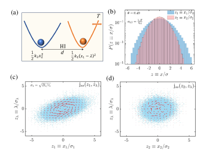
Figure 1: (a) Schematic of the hydrodynamically coupled particles in dual traps of different stiffness constants. The mean position of the trap with stiffness constant ‘$k_{1}$’ is modulated with an Ornstein-Uhlenbeck noise (‘$\lambda(t)$’) while the trap with stiffness constant ‘$k_{2}$’ remains unperturbed. $k_{1}=17.2\pm 0.2\ pN/\mu m$ and $k_{2}=12\pm 0.4\ pN/\mu m$ are fixed throughout the experiments. (b) The probability density functions of normalised positional fluctuations of the particles trapped in two traps ($d=4.2\ \mu m$) are plotted. The experimentally recorded fluctuations of both particles are normalised with the equilibrium standard deviations ($\sigma_{i}=\sqrt{k_{B}T/k_{i}}$) of corresponding traps. (c) The non-zero probability current corresponding to the particle in the driven trap is shown. (d) The probability current also appears to be non-zero corresponding to the particle in the fixed trap.

The dynamics of the system can be written as a multidimensional linear Langevin equation: $\mathbf{\dot{x}}(t)=-\mathbf{F}.\mathbf{x}(t)+\bm{\xi}(t)$, with $\langle\bm{\xi}(t):\bm{\xi}(t^{\prime})\rangle=2\delta(t-t^{\prime})\mathbf{D}$. Here, $\mathbf{x}(t)\equiv[x_{1}(t),x_{2}(t),\lambda(t)]^{T}$ consists of the fluctuating positions ($x_{1}(t),x_{2}(t)$) of the two particles measured with respect to the center of each optical traps having stiffness constants $k_{1}$ and $k_{2}$, and $\lambda(t)$ is the OU noise that is exponentially correlated with the relaxation timescale $\tau_{e}$ and amplitude $D_{e}$ with $\langle\lambda(t)\lambda(t^{\prime})\rangle=\frac{D_{e}}{\tau_{e}}\exp(-\frac{t-t^{\prime}}{\tau_{e}})$. The vector $\bm{\xi}(t)\equiv[\eta_{1}(t),\eta_{2}(t),\eta_{3}(t)]^{T}$ contains the random Brownian forces of the system. The drift ($\mathbf{F}$) and diffusion ($\mathbf{D}$) tensors can be expressed in terms of the hydrodynamic coupling constant $\epsilon\equiv\frac{3a}{2d}$ (considering first order of the Oseen tensor [18]) and the Stokes friction coefficient of the medium $\gamma\equiv 6\pi\eta a$ with viscosity $\eta$, such that

$$\mathbf{F}=\begin{pmatrix}k_{1}/\gamma&\epsilon k_{2}/\gamma&-k_{1}/\gamma\\ \epsilon k_{1}/\gamma&k_{2}/\gamma&-\epsilon k_{1}/\gamma\\ 0&0&\frac{1}{\tau_{e}}\end{pmatrix},\ \mathbf{D}=\begin{pmatrix}D_{0}&\epsilon D_{0}&0\\ \epsilon D_{0}&D_{0}&0\\ 0&0&\frac{D_{e}}{\tau_{e}^{2}}\end{pmatrix},$$ (1)

as $D_{0}=\frac{k_{B}T}{\gamma}$ ($k_{B}$ is the Boltzmann’s constant). The rationale behind the dynamical equations is explicitly discussed in SI .1.

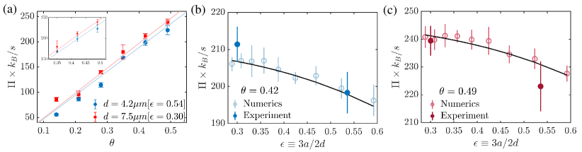
Figure 2: Entropy production rate ($\Pi$) of the ‘OU-noise driven model’: (a) Inferred $\Pi$ from the experimental data monotonically increases with the strength of the external noise (parametrised as $\theta$) at two different separations between the particles. The entropy production rate of the system decreases with the increasing hydrodynamic interaction ($\epsilon$) as shown for two different noise strengths (b) $\theta=0.42$ and (c) $\theta=0.49$. Corresponding theoretical estimations are shown with the solid lines.

A schematic of the system of our interest is shown in Fig.1(a). We primarily focus on the entropy production rate of the system after it reaches a nonequilibrium steady state defined by the joint probability distribution ($P_{ss}(\mathbf{x})$) and non-zero probability current ($\mathbf{j}_{ss}(\mathbf{x})$) corresponding to the whole phase space of the system. The marginal steady-state distributions of both the particles in the ‘driven’ ($x_{1}$) and ‘fixed’ ($x_{2}$) traps are Gaussian. The variance of the particle in the ‘driven’ trap is expectedly larger than the same in a fixed trap as shown in Fig.1(b) for a typical experimental trajectory. The recorded positional fluctuations of both particles are expressed as dimensionless quantities $z_{1,2}\equiv x_{1,2}/\sigma_{1,2}$ as $\sigma_{1,2}=\sqrt{k_{B}T/k_{1,2}}$. The non-zero probability current (as shown in Fig.1(c)) is strongly prevalent in $(x_{1},\lambda)$ space as the particle in the first trap is driven by the OU noise. However, the probability current also prevails in the $(x_{2},\lambda)$ space (Fig.1(d)), even though the external noise does not directly drive the particle in the second trap. This indicates the appearance of induced nonequilibrium dynamics through hydrodynamic interactions.

To check the effects of interactions, we perform the experiments at two different separations ($d=4.2\ \mu m$ and $d=7.5\ \mu m$) between the traps ($k_{1}=17.2\pm 0.2\ pN/\mu m$ and $k_{2}=12\pm 0.4\ pN/\mu m$) by varying the strength of the external noise (parameterized by $\theta=\frac{D_{e}/\tau_{e}^{2}}{D_{0}}$). Then we estimate the entropy production rate from the experimental and numerical data using the short-time inference technique [29, 30, 31, 26, 32] based on the thermodynamic uncertainty relation [33]. This technique is model-independent and particularly advantageous to estimate the entropy production rate from the experimental trajectories as it does not require any calibration factor to transform the measurements in positional units [26]. The technique is also briefly discussed in SI .2.

We find that the entropy production rate is monotonically increasing with $\theta$ at both separations (Fig.2(a)). However, the entropy generation rate for the separation $d=4.2\ \mu m$ at any $\theta$ is found to be slightly lower than the same for $d=7.5\ \mu m$ as shown in Fig.2(b) and Fig.2(c). This observation suggests that if the separation between two particles is reduced, the total entropy production rate of the system will also be decreased, even though the hydrodynamic coupling strength is enhanced in this process.

The analytically calculated total entropy production rate (in units of $k_{B}/s$) for the system [34],

$$\begin{split}\Pi=&\int d\mathbf{x}\frac{\mathbf{D}^{-1}\mathbf{j}_{ss}^{2}(\mathbf{x})}{P_{ss}(\mathbf{x})}\\ =&\frac{D_{e}k_{1}^{2}(\gamma+(1-\epsilon^{2})k_{2}\tau_{e})}{D_{0}\gamma\tau_{e}(\gamma^{2}+\gamma(k_{1}+k_{2})\tau_{e}+(1-\epsilon^{2})k_{1}k_{2}\tau_{e}^{2})},\end{split}$$ (2)

also corroborates our observation as shown in the plots of Fig.2. If the hydrodynamic interaction becomes negligible ($\epsilon\rightarrow 0$), the entropy production rate will be,

$$[\Pi]_{\epsilon\rightarrow 0}=\frac{D_{e}k_{1}^{2}}{D_{0}\gamma\tau_{e}(\gamma+k_{1}\tau_{e})},$$ (3)

which is greater than $\Pi$ - indicating the reduction of entropy production rate in the presence of hydrodynamic interactions. This occurs since the motion of the ‘driven’ particle gets constricted due to the other particle placed close to it - which results in a lower entropy production rate. Similar observations were made in Ref.[26] where the energy dissipation in a driven particle was found to be reduced due to hydrodynamic flows close to a microbubble.

Note that we could think of our two-particle system as a composite system consisting of the driven particle ($x_{1}$) - which has an intrinsic energy dissipation rate $[\Pi]_{\epsilon\rightarrow 0}$ - being the system of interest, and the other particle ($x_{2}$) being a probe brought close to it. This demonstrates that interactions with a probe, which by itself does not dissipate energy, could significantly reduce the energy dissipation to the environment from nonequilibrium systems.

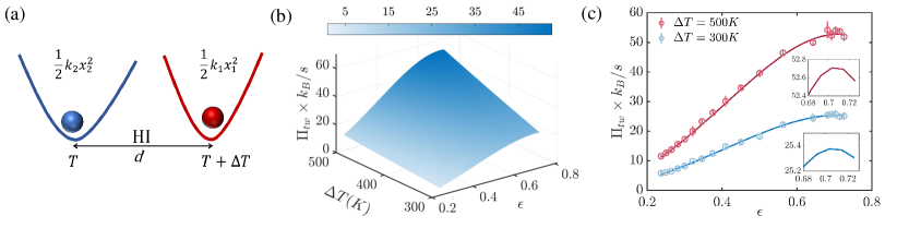
Figure 3: ‘Two-temperature model’: (a) Schematic of the hydrodynamically coupled particles in dual traps of different stiffness constants. The particle trapped in the potential with stiffness constant ‘$k_{1}$’ is in temperature $T+\Delta T$ while the particle in the trap with stiffness constant ‘$k_{2}$’ remains in temperature $T$. (b) Theoretical estimation of the entropy production rate of the system is plotted with $\Delta T$ and hydrodynamic coupling strength $\epsilon$. [$k_{1}=17.2pN/\mu m$, $k_{2}=12pN/\mu m$] (c) Estimation of entropy production rate as a function of $\epsilon$ - using the short-time inference scheme from numerical trajectories of the system for fixed $\Delta T$. The solid lines indicate corresponding theoretical predictions. The non-monotonic feature of $\Pi_{tw}$ with $\epsilon$ is shown as the insets.

Additionally, it is important to note that the energy balance of the interacting system should hold such that input power estimated as, $\langle\dot{W}\rangle=k_{1}\langle\lambda(t)\circ\dot{x}_{1}(t)\rangle$ is exactly equal to the total dissipated heat.This can be easily computed from the increase in entropy of the medium as $-\langle\dot{Q}\rangle=-\langle Q_{1}+Q_{2}\rangle=k_{B}T\Pi_{m}\equiv k_{B}T\langle\mathbf{D}^{-1}\mathbf{(Fx)\circ\dot{x}}\rangle$) (see SI .3 for the details of the calculation). Note that it would not have been possible to establish energy balance in this system through the approach of applying trajectory energetics to langevin equations of individual variables, as has been previously done in Refs. [35, 36, 37, 38]. Since the thermal noises involved in hydrodynamically coupled systems are cross-correlated (this leads to the non-diagonal form of the diffusion matrix), defining heat flow at the subsystem level ($Q_{1}$ and $Q_{2}$) for this system still remains unclear  [16].

Next, we theoretically discuss the role of hydrodynamic interactions in a system of two particles where the particles are at different temperatures. We call this model the ‘two-temperature model’ for further discussion. The dynamics of this system can be similarly expressed as a coupled Langevin equation with drift ($\mathbf{F}_{tw}$) and diffusion ($\mathbf{D}_{tw}$) tensors of following forms [35] -

$$\mathbf{F}_{tw}=\begin{pmatrix}k_{1}/\gamma&\epsilon k_{2}/\gamma\\ \epsilon k_{1}/\gamma&k_{2}/\gamma\\ \end{pmatrix},\ \mathbf{D}_{tw}=\begin{pmatrix}\frac{k_{B}(T+\Delta T)}{\gamma}&\epsilon\frac{k_{B}(T+\Delta T)}{\gamma}\\ \epsilon\frac{k_{B}(T+\Delta T)}{\gamma}&\frac{k_{B}(T+\epsilon^{2}\Delta T)}{\gamma}\\ \end{pmatrix},$$ (4)

where the particle in the trap of stiffness $k_{1}$ feels the temperature $T+\Delta T$ and the other particle in the trap of stiffness $k_{2}$ feels a lower temperature $T$. The underlying rationale for the dynamical equations of this system is elegantly explained in Refs. [35, 39]. This model is also experimentally viable and studied in detail in several Refs. [35, 36]. In these studies, the two-temperature configuration was created by forcing one of the particles by random white noise while the other particle was kept in close proximity. The effect of the random white noise is assimilated as an ‘effective temperature’ which is attributed to the different temperatures of the two particles. The total entropy production rate of this system can be analytically computed as (with the same formalism used for the ‘OU-noise driven model’),

$$\Pi_{tw}=\frac{k_{2}^{2}\Delta T^{2}\epsilon^{2}(1-\epsilon^{2})}{(k_{1}+k_{2})\gamma T(T+\Delta T)},$$ (5)

and is found to be non-monotonic in $\epsilon$ with a maxima at $\epsilon=1/\sqrt{2}\equiv 0.707$ as shown in Fig.3(b) and Fig.3(c). This indicates that the entropy production rate of the system is enhanced with the increased hydrodynamic coupling up to a certain separation before it goes down even though the interaction is enhanced.

Interestingly, by combining this formula with the energy balance condition, we can straightforwardly obtain an expression for the rate of heat dissipated by the hot particle $=-\langle\dot{Q}_{1}\rangle$ (which, if energy balance holds, will be the same as the heat absorbed by the cold particle $\langle\dot{Q}_{2}\rangle$ with a minus sign) as,

$$\begin{split}\langle\dot{Q}_{1}\rangle=-\langle\dot{Q}_{2}\rangle&=k_{B}\frac{\Pi_{tw}}{\frac{1}{T}-\frac{1}{T+\Delta T}},\\ &=\frac{k_{2}^{2}\epsilon^{2}(1-\epsilon^{2})}{(k_{1}+k_{2})\gamma}k_{B}\Delta T\\ &\equiv-\langle\dot{Q}\rangle.\end{split}$$ (6)

Note that this approach was not taken in previous studies, and it was argued that there is a violation of the First Law in such systems with some amount of heat being lost in interactions, except for the case where $k_{1}=k_{2}$  [36, 37]. We, however, compute the entropy production rate and assume that the First Law should hold, which enables us to obtain an expression for heat consistently. The derived expression is the same as the expression for heat flow from hot particle to cold particle previously obtained in Refs. [36, 37]. In addition, we argue that the estimated heat flow needs to be entirely associated with the heat dissipated by the hot particle, as well as the heat absorbed by the cold particle such that the energy balance condition is automatically satisfied (See SI .3 for further details).

This system will reach an equilibrium steady state if the two particles are well-separated with negligible hydrodynamic interaction. The hydrodynamic interaction combined with the difference in temperatures breaks the detailed balance, resulting in the transfer of heat from the relatively ‘hot’ particle to the ‘cold’ one as the particles are placed closer to each other. If the separation between particles is so small that the motion of the particles is affected, the entropy production rate decreases, resulting in a non-monotonic dependence of entropy production on the interaction strength.

As a corollary, note that - considering either one of the interacting particles as a probe (having interactions with the other) - our particular system highlights the importance of ensuring that the probe’s temperature matches that of the system. This guarantees that the interaction with the probe alone does not make the system appear out of equilibrium, not does it add additional contributions to dissipation.

Conclusions.- In conclusion, we unravel the effects of hydrodynamic interactions influencing the irreversibility of two mesoscopic systems with different origins of nonequilibrium characteristics. We specifically find that the entropy production rate shows completely different features for the two systems as a function of the strength of the hydrodynamic interactions. Moreover, we resolve the issues related to the energy balance for hydrodynamically coupled systems with the energetics estimated directly from the entropy production rate.

Our observations suggest that even first-order interactions between subsystems can bring forth surprising behaviours in the irreversibility of a system with only a few degrees of freedom. In this context, the details of the dynamics are crucial in discerning the role of certain interactions in nonequilibrium systems with multiple reservoirs or co-evolving degrees of freedom in a single heat bath. Notably, it will be interesting to test the effects of higher-order interactions on the irreversibility of out-of-equilibrium processes in similar steady states as well as in different time-dependent configurations [40]. Also, the impact of such interactions in the context of information transfer in biochemical signalling networks [41, 42] and optimising protocols for non-equilibrium control problems [43, 44, 45] will be quite interesting to investigate.

Acknowledgements.-The work is supported by IISER Kolkata, an autonomous teaching and research institute supported by the Ministry of Education, Government of India, and the Science and Engineering Research Board, Department of Science and Technology, Government of India, through the research grant CRG/2022/002417. BD is thankful to the Ministry Of Education of Government of India for financial support through the Prime Minister’s Research Fellowship (PMRF) grant. SKM acknowledges the Knut and Alice Wallenberg Foundation for financial support through Grant No. KAW 2021.0328. S.K acknowledges the support of the Swedish Research Council through the grant 2021-05070.

Supplementary Materials

.1 OU-noise driven model: Dynamical descriptions

The dynamics of the two identical microscopic particles (radius $a$) trapped in parabolic potentials separated by a distance $d$ with different stiffness constants $k_{1}$ and $k_{2}$ can be expressed by a coupled $Langevin$ equation [17, 36, 19],

$$\begin{split}\dot{x}_{1}(t)=&\mathcal{H}_{11}[-k_{1}x_{1}(t)+\xi_{1}(t)]+\mathcal{H}_{12}[-k_{2}x_{2}(t)+\xi_{2}(t)]\\ \dot{x}_{2}(t)=&\mathcal{H}_{21}[-k_{1}x_{1}(t)+\xi_{1}(t)]+\mathcal{H}_{22}[-k_{2}x_{2}(t)+\xi_{2}(t)],\end{split}$$ (7)

where $\mathcal{H}_{ij}$ $(i,j=1,2)$ are the constant elements of a hydrodynamic coupling tensor of the form $\mathbf{\mathcal{H}}=\begin{pmatrix}1/\gamma&\epsilon/\gamma\\ \epsilon/\gamma&1/\gamma\\ \end{pmatrix}$ - considering that the displacements of the particles ($x_{1}(t)$, $x_{2}(t)$) are small compared to the mean separation between the traps ($d$). Here $\epsilon\equiv\frac{3a}{2d}$ denotes the coupling coefficient taken as the lower order component of the Oseen tensor [17, 18] for longitudinal motions and $\gamma\equiv 6\pi\eta a$ is the viscous drag coefficient of the medium. The terms $\xi_{1}(t)$ and $\xi_{2}(t)$ are delta-correlated random Brownian forces such that $\langle\xi_{i}(t)\rangle=0,\ \langle\xi_{i}(t)\xi_{j}(t)\rangle=2k_{B}T(\mathcal{H})^{-1}_{ij}\delta(t-t^{\prime})$. $k_{B}$ is the Boltzmann’s constant.

Without any external perturbation, the coupled particles will be in thermal equilibrium with the bath of temperature $T$. Following Ref. [35], Eq.(7) can be rewritten as,

$$\begin{split}\dot{x}_{1}(t)&=b_{1}(x_{1}(t),x_{2}(t))+\eta_{1}(t)\\ \dot{x}_{2}(t)&=b_{2}(x_{1}(t),x_{2}(t))+\eta_{2}(t),\end{split}$$ (8)

with

$$\begin{split}b_{i}(x_{i},x_{j})&=-\frac{1}{\gamma}k_{i}x_{i}-\frac{\epsilon}{\gamma}k_{j}x_{j},\\ \eta_{1}&=\frac{1}{\gamma}(\xi_{1}+\epsilon\xi_{2}),\\ \eta_{2}&=\frac{1}{\gamma}(\xi_{2}+\epsilon\xi_{1}).\end{split}$$ (9)

The Fokker-Planck equation corresponding to the time evolution of the joint probability distribution ($\rho_{eq}(x_{1},x_{2},t)$) of this (thermally) equilibrium configuration can be written as,

$$\partial_{t}\rho_{eq}(x_{1},x_{2},t)=-\partial_{x_{1}}(b_{1}\rho_{eq})-\partial_{x_{2}}(b_{2}\rho_{eq})+\alpha_{11}\partial_{x_{1}}^{2}\rho_{eq}+\alpha_{22}\partial_{x_{2}}^{2}\rho_{eq}+2\alpha_{12}\partial_{x_{1}x_{2}}^{2}\rho_{eq},$$ (10)

with $\alpha_{11}=\alpha_{22}\equiv\frac{k_{B}T}{\gamma}$ and $\alpha_{12}=\alpha_{21}\equiv\epsilon\frac{k_{B}T}{\gamma}$ are the elements of the equilibrium diffusion matrix ($\mathbf{D}_{eq}$) of the system such that $\langle\eta_{i}(t)\eta_{j}(t^{\prime})\rangle=2(\mathbf{D}_{eq})_{ij}\delta(t-t^{\prime})$.

To drive the system out of equilibrium, the particle trapped in the potential with stiffness constant $k_{1}$ is modulated with an Ornstein-Uhlenbeck (OU) noise ($\lambda(t)$). The external modulation is exponentially correlated with the relaxation timescale $\tau_{e}$ and amplitude $D_{e}$ as $\langle\lambda(t)\lambda(t^{\prime})\rangle=\frac{D_{e}}{\tau_{e}}\exp(-\frac{t-t^{\prime}}{\tau_{e}})$ and it is derivable from following dynamical equation,

$$\dot{\lambda}(t)=-\frac{\lambda(t)}{\tau_{e}}+\frac{\sqrt{2D_{e}}}{\tau_{e}}\eta_{3}(t),~{}~{}~{}~{}~{}\langle\eta_{3}(t)\rangle=0,\langle\eta_{3}(t)\eta_{3}(t^{\prime})\rangle=\delta(t-t^{\prime}).$$ (11)

Now, the dynamics of the perturbed system with the external OU modulation can be expressed with a system of Langevin equations with $\lambda(t)$ as another degree of freedom in addition to $x_{1}(t)$ and $x_{2}(t)$ such that,

$$\begin{split}\dot{x}_{1}(t)=&\mathcal{H}_{11}[-k_{1}(x_{1}(t)-\lambda(t))+\xi_{1}(t)]+\mathcal{H}_{12}[-k_{2}x_{2}(t)+\xi_{2}(t)]\\ \dot{x}_{2}(t)=&\mathcal{H}_{21}[-k_{1}(x_{1}(t)-\lambda(t))+\xi_{1}(t)]+\mathcal{H}_{22}[-k_{2}x_{2}(t)+\xi_{2}(t)]\\ \dot{\lambda}(t)=&-\frac{\lambda(t)}{\tau_{e}}+\frac{\sqrt{2D_{e}}}{\tau_{e}}\eta_{3}(t).\end{split}$$ (12)

Here, $\langle\xi_{1}(t)\eta_{3}(t^{\prime})\rangle=\langle\xi_{2}(t)\eta_{3}(t^{\prime})\rangle=0\implies\langle\eta_{1}(t)\eta_{3}(t^{\prime})\rangle=\langle\eta_{2}(t)\eta_{3}(t^{\prime})\rangle=0$. Moreover, Eq.(12) can be rewritten in the following matrix form,

$$\begin{pmatrix}\dot{x}_{1}(t)\\ \dot{x}_{2}(t)\\ \dot{\lambda}(t)\end{pmatrix}=-\begin{pmatrix}k_{1}/\gamma&\epsilon k_{2}/\gamma&-k_{1}/\gamma\\ \epsilon k_{1}/\gamma&k_{2}/\gamma&-\epsilon k_{1}/\gamma\\ 0&0&\frac{1}{\tau_{e}}\end{pmatrix}\begin{pmatrix}x_{1}(t)\\ x_{2}(t)\\ \lambda(t)\end{pmatrix}+\begin{pmatrix}\eta_{1}(t)\\ \eta_{2}(t)\\ \eta_{3}(t)\end{pmatrix}$$ (13)

$$\implies\mathbf{\dot{x}(t)}=-\mathbf{F}.\mathbf{x(t)}+\bm{\xi(t)},$$ (14)

with $\langle\bm{\xi}(t):\bm{\xi}(t^{\prime})\rangle=2\delta(t-t^{\prime})\mathbf{D}$. Therefore, the drift ($\mathbf{F}$) and diffusion ($\mathbf{D}$) matrices for the ‘OU-noise driven model’ are of following forms,

$$\mathbf{F}=\begin{pmatrix}k_{1}/\gamma&\epsilon k_{2}/\gamma&-k_{1}/\gamma\\ \epsilon k_{1}/\gamma&k_{2}/\gamma&-\epsilon k_{1}/\gamma\\ 0&0&\frac{1}{\tau_{e}}\end{pmatrix},\ \mathbf{D}=\begin{pmatrix}D_{0}&\epsilon D_{0}&0\\ \epsilon D_{0}&D_{0}&0\\ 0&0&\frac{D_{e}}{\tau_{e}^{2}}\end{pmatrix},$$ (15)

with $D_{0}=\frac{k_{B}T}{\gamma}$.

Steady state distribution.- The probability of finding the particle in a configuration $\mathbf{x}$ at a certain time $t$ can be determined in terms of probability distribution function $P(\mathbf{x},t)$ which follows the Fokker-plank equation of the form

$$\begin{split}\partial_{t}P(\mathbf{x},t)&=-\nabla\cdot(-\mathbf{F}\mathbf{x}P({\mathbf{x},t})-\mathbf{D}\nabla P(\mathbf{x},t))\\ &\equiv-\nabla\cdot\mathbf{j}(\mathbf{x},t)\end{split}$$ (16)

where, $\mathbf{j}(\mathbf{x},t)$ denotes the probability current in the phase space.

Starting from an arbitrary initial condition for $\mathbf{x}$, the system will reach a non-equilibrium steady state in the long time ($\lim t\rightarrow\infty$) with a characteristic probability distribution and current given by,

$$\begin{split}P_{ss}(\mathbf{x})=(2\pi\sqrt{\det\mathbf{C}})^{-1}e^{-\frac{1}{2}\mathbf{x}^{T}\mathbf{C}^{-1}\mathbf{x}}\\ \mathbf{j}_{ss}(\mathbf{x})=(-\mathbf{F}\mathbf{x}+\mathbf{D}\mathbf{C}^{-1}\mathbf{x})P_{ss}(\mathbf{x}),\end{split}$$ (17)

in terms of the long-time limit of the covariance matrix $\mathbf{C}(t)$.
Covariance matrix.- Note that the diffusion tensor is not proportional to an identity matrix as $D_{ii}\neq D_{jj},D_{ij}\neq 0$, which indicates the system to be non-multipartite [16]. Following the technique introduced in [46], the steady-state covariance matrix $\mathbf{C}$ is given by

$$\mathbf{C}=\mathbf{F}^{-1}(\mathbf{D}+\mathbf{Q}),$$ (18)

where $\mathbf{Q}$ is an antisymmetric $3\times 3$ matrix that can be uniquely determined by

$$\mathbf{FQ}+\mathbf{QF}^{T}=\mathbf{FD}-\mathbf{DF}^{T}.$$ (19)

If $\mathbf{Q}$ is nonzero in the NESS, it implies the violation of the detailed balance in the system. Now the elements of the steady state ($\lim t\rightarrow\infty$) covariance matrix for this system will be,

$$\begin{split}&C_{11}\equiv\langle x_{1}x_{1}\rangle=\frac{D_{0}\gamma}{k_{1}}+\frac{D_{e}k_{1}(\gamma(k_{1}+k_{2}-\epsilon^{2}k_{2})+(1-\epsilon^{2})k_{2}(k_{1}+k_{2})\tau_{e})}{(k_{1}+k_{2})(\gamma^{2}+\gamma(k_{1}+k_{2})\tau_{e}+(1-\epsilon^{2})k_{1}k_{2}\tau_{e}^{2})},\\ &C_{12}\equiv\langle x_{1}x_{2}\rangle=\frac{\epsilon D_{e}\gamma k_{1}^{2}}{(k_{1}+k_{2})(\gamma^{2}+\gamma(k_{1}+k_{2})\tau_{e}+(1-\epsilon^{2})k_{1}k_{2}\tau_{e}^{2})},\\ &C_{13}\equiv\langle x_{1}\lambda\rangle=\frac{D_{e}k_{1}(\gamma+(1-\epsilon^{2})k_{2}\tau_{e})}{(\gamma^{2}+\gamma(k_{1}+k_{2})\tau_{e}+(1-\epsilon^{2})k_{1}k_{2}\tau_{e}^{2})},\\ &C_{21}\equiv\langle x_{2}x_{1}\rangle=C_{12},\\ &C_{22}\equiv\langle x_{2}x_{2}\rangle=\frac{D_{0}\gamma}{k_{2}}+\frac{\epsilon^{2}D_{e}\gamma k_{1}^{2}}{(k_{1}+k_{2})(\gamma^{2}+\gamma(k_{1}+k_{2})\tau_{e}+(1-\epsilon^{2})k_{1}k_{2}\tau_{e}^{2})},\\ &C_{23}\equiv\langle x_{2}\lambda\rangle=\frac{\epsilon D_{e}\gamma k_{1}}{\gamma^{2}+\gamma(k_{1}+k_{2})\tau_{e}+(1-\epsilon^{2})k_{1}k_{2}\tau_{e}^{2}},\\ &C_{31}\equiv\langle\lambda x_{1}\rangle=C_{13},\\ &C_{32}\equiv\langle\lambda x_{2}\rangle=C_{23},\\ &C_{33}\equiv\langle\lambda\lambda\rangle=\frac{D_{e}}{\tau_{e}}.\end{split}$$ (20)

If the particles are well separated such that hydrodynamic coupling is negligible ($\epsilon\rightarrow 0$), the covariance matrix will be,

$$\mathbf{C}=\begin{pmatrix}\frac{D_{0}\gamma}{k_{1}}+\frac{D_{e}k_{1}}{\gamma+k_{1}\tau_{e}}&0&\frac{D_{e}k_{1}}{\gamma+k_{1}\tau_{e}}\\ 0&\frac{D_{0}\gamma}{k_{2}}&0\\ \frac{D_{e}k_{1}}{\gamma+k_{1}\tau_{e}}&0&\frac{D_{e}}{\tau_{e}}\end{pmatrix}$$ (21)

Moreover, we can find the covariance matrix corresponding to the out-of-equilibrium situation with the hydrodynamic coupling where the external modulation is Gaussian white noise - by taking $\tau_{e}\rightarrow 0$ (with $D_{e}\neq 0$) in Eq.(20),

$$\begin{split}&[C_{11}]_{tw}=\frac{D_{0}\gamma}{k_{1}}+\frac{D_{e}k_{1}^{2}}{\gamma k_{1}}-\epsilon^{2}\frac{k_{2}}{k_{1}}\frac{D_{e}k_{1}^{2}}{\gamma(k_{1}+k_{2})},\\ &[C_{12}]_{tw}=\epsilon\frac{D_{e}k_{1}^{2}}{\gamma(k_{1}+k_{2})},\\ &[C_{22}]_{tw}=\frac{D_{0}\gamma}{k_{2}}+\epsilon^{2}\frac{D_{e}k_{1}^{2}}{\gamma(k_{1}+k_{2})}.\end{split}$$ (22)

If we consider $D_{e}k_{1}^{2}=k_{B}\Delta T\gamma$ to match the noise correlation of the external Gaussian modulation of Ref. [35], Eqs.(22) will be transformed to,

$$\begin{split}&[C_{11}]_{tw}=\frac{k_{B}T}{k_{1}}+\frac{k_{B}\Delta T}{k_{1}}-\epsilon^{2}\frac{k_{2}}{k_{1}}\frac{k_{B}\Delta T}{(k_{1}+k_{2})},\\ &[C_{12}]_{tw}=\epsilon\frac{k_{B}\Delta T}{(k_{1}+k_{2})},\\ &[C_{22}]_{tw}=\frac{k_{B}T}{k_{2}}+\epsilon^{2}\frac{k_{B}\Delta T}{(k_{1}+k_{2})},\end{split}$$ (23)

which match exactly with the Eqs.(14) of Ref.[35]. Moreover, Eq. (23) are the elements of the steady state covariance matrix of the ‘two-temperature model’ we discussed in the main text.

It is also clear that the steady-state cross-variances will be non-zero only in the out-of-equilibrium configuration. In an equilibrium situation ($D_{e}=0$ or $\Delta T=0$), the two particles will be statistically independent with the variance $\frac{k_{B}T}{k_{1}}$ and $\frac{k_{B}T}{k_{2}}$ respectively.

.2 Entropy production rate and Short-time inference technique

The entropy production rate for a nonequilibrium system in a steady state with the probability density $\rho_{ss}(\mathbf{x})$ and current $\mathbf{j}_{ss}(\mathbf{x})$ is analytically estimated as [34]

$$\Pi=\int d\mathbf{x}\frac{\mathbf{D}^{-1}\mathbf{j}_{ss}^{2}(\mathbf{x})}{P_{ss}(\mathbf{x})},$$ (24)

which we use to compute the entropy production rate for both models and discuss their dependency on the interaction strength. However, estimating the entropy production rate from the experimental or numerical trajectories is nontrivial using the above formula. We have used an indirect technique based on the thermodynamic uncertainty relation [33]. The short-time inference technique was first introduced for overdamped $Langevin$ dynamics in Ref. [29] and rigorously proved in Refs. [30, 31]. It was subsequently used to estimate the entropy production rate from experimental trajectories in Ref. [26]. Moreover, this technique is effectively applicable to systems with nonlinear potential landscapes [32] and to inferring the activity of biological cells [47]. Using this technique, we can estimate the entropy production rate of a system in a non-equilibrium steady state as

$$\Pi=\lim_{dt\rightarrow 0}\max_{J}\left[\frac{2k_{B}\langle J\rangle^{2}}{dt\ \text{Var}(J)}\right],$$ (25)

where $J$ is a weighted scalar current - that can be computed from the time discretized experimental or numerical trajectory data ($\mathbf{x}^{i}$) sampled at an interval of $dt$ - as

$$J=\mathbf{f}\left(\frac{\mathbf{x}^{i+1}+\mathbf{x}^{i}}{2}\right)\cdot\left(\mathbf{x}^{i+1}-\mathbf{x}^{i}\right).$$ (26)

Motivated by the linearity of the systems, we have approximated $\mathbf{f(x)}$ as the linear combination of linear basis functions $\psi_{m}(\mathbf{x})$ of different dimensions (equal to the number of degrees of freedom considered in a model) as $\mathbf{f(x)}=\sum_{m=1}^{M}\mathbf{a}_{m}\psi_{m}(\mathbf{x})$. For any such adequate representation of $\mathbf{f(x)}$, an analytical solution to the maximisation problem of Eq.(25) is known [30] and given by,

$$\Pi=\frac{2\langle\psi_{k}\rangle(\bm{\Xi}^{-1})_{k,l}\langle\psi_{l}\rangle}{dt},$$ (27)

where, $(\bm{\Xi})_{k,l}=\langle\psi_{k}\psi_{l}\rangle-\langle\psi_{k}\rangle\langle\psi_{l}\rangle$. To find more details about the method, we refer to Sec. II B of Ref. [30] and to Sec. III of Ref. [32].

.3 Validation of thermodynamic laws

For the ‘OU-noise driven model’, the input power can be estimated as,

$$\begin{split}\langle\dot{W}\rangle=&k_{1}\langle\lambda(t)\circ\dot{x}_{1}(t)\rangle\\ =&\frac{D_{e}k_{1}^{2}(\gamma+(1-\epsilon^{2})k_{2}\tau_{e})}{\tau_{e}(\gamma^{2}+\gamma(k_{1}+k_{2})\tau_{e}+(1-\epsilon^{2})k_{1}k_{2}\tau_{e}^{2})},\end{split}$$ (28)

which should be exactly equal to the total rate of heat flow between the particles to validate the first law of thermodynamics. since there is no change in the internal energy of the particles in a steady state. However, we find that heat fluxes due to the respective particles, defined as $Q_{i}(t_{m})=\int_{0}^{t_{m}}dt\ (\gamma\dot{x}_{i}-\eta_{i})\circ\dot{x}_{i}$, do not add up to the total input power of the system. Since the thermal noises involved in hydrodynamically coupled systems are cross-correlated (this leads to the non-diagonal form of the diffusion matrix), defining heat flow at the subsystem level for a system with even few degrees of freedom is not at all straightforward  [16] and that may lead to the wrong estimation of the total rate of heat flow defined as a direct sum of such heat fluxes corresponding to the individual subsystems. To avoid the anomaly regarding the first law of thermodynamics, it will be useful to look at the increase in entropy of the medium as it directly relates to the heat dissipation of a steady-state system [34, 16] such that,

$$\begin{split}\frac{\langle\dot{Q}\rangle}{k_{B}T}=&\Pi_{m}\equiv\langle\mathbf{D}^{-1}\mathbf{(Fx)\circ\dot{x}}\rangle\\ \implies\Pi_{m}=&\int d\mathbf{x}\ \mathbf{D}^{-1}\mathbf{(Fx)}\mathbf{j}_{ss}(\mathbf{x}).\end{split}$$ (29)

The medium entropy production rate for the ‘OU-noise driven model’ is estimated to be,

$$\begin{split}\Pi_{m}=&-\frac{D_{e}k_{1}^{2}(\gamma+(1-\epsilon^{2})k_{2}\tau_{e})}{D_{0}\gamma\tau_{e}(\gamma^{2}+\gamma(k_{1}+k_{2})\tau_{e}+(1-\epsilon^{2})k_{1}k_{2}\tau_{e}^{2})},\\ \implies\langle\dot{Q}\rangle=&D_{0}\gamma\Pi_{m}\\ =&-\frac{D_{e}k_{1}^{2}(\gamma+(1-\epsilon^{2})k_{2}\tau_{e})}{\tau_{e}(\gamma^{2}+\gamma(k_{1}+k_{2})\tau_{e}+(1-\epsilon^{2})k_{1}k_{2}\tau_{e}^{2})},\end{split}$$ (30)

as $D_{0}\gamma=k_{B}T$. It is now evident that the estimated heat dissipation validates the first law of thermodynamics as, $-\langle\dot{Q}\rangle=\langle\dot{W}\rangle$ [Eq. (28) with appropriate sign convention].

For the ‘two-temperature model’, heat fluxes due to the respective particles was estimated as $Q_{i}(t_{m})=\int_{0}^{t_{m}}dt\ (\gamma\dot{x}_{i}-\eta_{i})\circ\dot{x}_{i}$ in Refs. [35, 36, 37]. These studies showed that the heat released from the ‘hot’ particle was not fully exhausted by the ‘cold’ one if the particles were trapped in potentials with different stiffnesses - leading to the ‘apparent’ violation of the energy balance relation. It was also indicated that energy would not be conserved for this system due to the dissipative nature of the coupling and energy conservation could be restored if the two particles are trapped in potentials with equal stiffnesses as the system will then be indistinguishable from those with conservative coupling [37].

Here we compute the heat fluxes of the particles from the knowledge of the total entropy production rate of the system. If the rate of heat dissipated by the ‘hot’ particle is $\langle\dot{Q}_{1}\rangle$ and the rate of heat absorbed by the ‘cold’ particle is $\langle\dot{Q}_{2}\rangle$, the total entropy production rate for the system ($\Pi_{tw}$) in NESS will be,

$$\Pi_{tw}=-\frac{\langle\dot{Q}_{1}\rangle}{k_{B}(T+\Delta T)}-\frac{\langle\dot{Q}_{2}\rangle}{k_{B}T}.$$ (31)

Now, according to the energy balance condition, $-\langle\dot{Q}_{1}\rangle=\langle\dot{Q}_{2}\rangle=\langle\dot{Q}\rangle$. So Eq. (31) reduces to,

$$\begin{split}-\langle\dot{Q}\rangle\left(\frac{1}{T}-\frac{1}{T+\Delta T}\right)=k_{B}\Pi_{tw}\\ \implies\langle\dot{Q}\rangle=-k_{B}\Pi_{tw}\frac{T(T+\Delta T)}{\Delta T}\\ =-\frac{k_{2}^{2}\epsilon^{2}(1-\epsilon^{2})}{(k_{1}+k_{2})\gamma}k_{B}\Delta T.\end{split}$$ (32)

The derived expression is the same as the expression for heat flow from hot particle to cold particle previously obtained in Refs. [36, 37]. However, in addition, we argue that it needs to be entirely associated with the heat dissipated by the hot particle, and the heat absorbed by the cold particle such that the energy balance condition is automatically satisfied.

References

- Seifert [2012] U. Seifert, Stochastic thermodynamics, fluctuation theorems and molecular machines, Reports on Progress in Physics 75, 126001 (2012).
- Seifert [2019] U. Seifert, From stochastic thermodynamics to thermodynamic inference, Annual Review of Condensed Matter Physics 10, 171 (2019).
- Roldán and Parrondo [2010] É. Roldán and J. M. Parrondo, Estimating dissipation from single stationary trajectories, Physical Review Letters 105, 150607 (2010).
- Sagués et al. [2007] F. Sagués, J. M. Sancho, and J. García-Ojalvo, Spatiotemporal order out of noise, Reviews of Modern Physics 79, 829 (2007).
- Howes et al. [2014] P. D. Howes, R. Chandrawati, and M. M. Stevens, Colloidal nanoparticles as advanced biological sensors, Science 346, 1247390 (2014).
- Alivisatos [2004] P. Alivisatos, The use of nanocrystals in biological detection, Nature Biotechnology 22, 47 (2004).
- Gnesotto et al. [2018] F. S. Gnesotto, F. Mura, J. Gladrow, and C. P. Broedersz, Broken detailed balance and non-equilibrium dynamics in living systems: a review, Reports on Progress in Physics 81, 066601 (2018).
- Mizuno et al. [2007] D. Mizuno, C. Tardin, C. F. Schmidt, and F. C. MacKintosh, Nonequilibrium mechanics of active cytoskeletal networks, Science 315, 370 (2007).
- Stuhrmann et al. [2012] B. Stuhrmann, M. S. e Silva, M. Depken, F. C. MacKintosh, and G. H. Koenderink, Nonequilibrium fluctuations of a remodeling in vitro cytoskeleton, Physical Review E 86, 020901 (2012).
- Bacanu et al. [2023] A. Bacanu, J. F. Pelletier, Y. Jung, and N. Fakhri, Inferring scale-dependent non-equilibrium activity using carbon nanotubes, Nature Nanotechnology 18, 905 (2023).
- Seyforth et al. [2022] H. Seyforth, M. Gomez, W. B. Rogers, J. L. Ross, and W. W. Ahmed, Nonequilibrium fluctuations and nonlinear response of an active bath, Physical Review Research 4, 023043 (2022).
- Turlier et al. [2016] H. Turlier, D. A. Fedosov, B. Audoly, T. Auth, N. S. Gov, C. Sykes, J.-F. Joanny, G. Gompper, and T. Betz, Equilibrium physics breakdown reveals the active nature of red blood cell flickering, Nature Physics 12, 513 (2016).
- Di Terlizzi et al. [2024] I. Di Terlizzi, M. Gironella, D. Herráez-Aguilar, T. Betz, F. Monroy, M. Baiesi, and F. Ritort, Variance sum rule for entropy production, Science 383, 971 (2024).
- Lynn et al. [2022a] C. W. Lynn, C. M. Holmes, W. Bialek, and D. J. Schwab, Decomposing the local arrow of time in interacting systems, Physical Review Letters 129, 118101 (2022a).
- Lynn et al. [2022b] C. W. Lynn, C. M. Holmes, W. Bialek, and D. J. Schwab, Emergence of local irreversibility in complex interacting systems, Physical Review E 106, 034102 (2022b).
- Leighton and Sivak [2024] M. P. Leighton and D. A. Sivak, Jensen bound for the entropy production rate in stochastic thermodynamics, Physical Review E 109, L012101 (2024).
- Meiners and Quake [1999] J.-C. Meiners and S. R. Quake, Direct measurement of hydrodynamic cross correlations between two particles in an external potential, Physical Review Letters 82, 2211 (1999).
- Herrera-Velarde et al. [2013] S. Herrera-Velarde, E. C. Euán-Díaz, F. Córdoba-Valdés, and R. Castaneda-Priego, Hydrodynamic correlations in three-particle colloidal systems in harmonic traps, Journal of Physics: Condensed Matter 25, 325102 (2013).
- Paul et al. [2017] S. Paul, A. Laskar, R. Singh, B. Roy, R. Adhikari, and A. Banerjee, Direct verification of the fluctuation-dissipation relation in viscously coupled oscillators, Physical Review E 96, 050102 (2017).
- Paul et al. [2019] S. Paul, R. Kumar, and A. Banerjee, A quantitative analysis of memory effects in the viscously coupled dynamics of optically trapped brownian particles, Soft Matter 15, 8976 (2019).
- Yuan and Tanaka [2024] J. Yuan and H. Tanaka, Impact of hydrodynamic interactions on the kinetic pathway of protein folding, Physical Review Letters 132, 138402 (2024).
- Kotar et al. [2010] J. Kotar, M. Leoni, B. Bassetti, M. C. Lagomarsino, and P. Cicuta, Hydrodynamic synchronization of colloidal oscillators, Proceedings of the National Academy of Sciences 107, 7669 (2010).
- Curran et al. [2012] A. Curran, M. P. Lee, M. J. Padgett, J. M. Cooper, and R. Di Leonardo, Partial synchronization of stochastic oscillators through hydrodynamic coupling, Physical Review Letters 108, 240601 (2012).
- Gomez-Solano et al. [2010] J. R. Gomez-Solano, L. Bellon, A. Petrosyan, and S. Ciliberto, Steady-state fluctuation relations for systems driven by an external random force, Europhysics Letters 89, 60003 (2010).
- Pal and Sabhapandit [2013] A. Pal and S. Sabhapandit, Work fluctuations for a brownian particle in a harmonic trap with fluctuating locations, Physical Review E 87, 022138 (2013).
- Manikandan et al. [2021] S. K. Manikandan, S. Ghosh, A. Kundu, B. Das, V. Agrawal, D. Mitra, A. Banerjee, and S. Krishnamurthy, Quantitative analysis of non-equilibrium systems from short-time experimental data, Communications Physics 4, 258 (2021).
- Das et al. [2023] B. Das, S. Paul, S. K. Manikandan, and A. Banerjee, Enhanced directionality of active processes in a viscoelastic bath, New Journal of Physics 25, 093051 (2023).
- Bera et al. [2017] S. Bera, S. Paul, R. Singh, D. Ghosh, A. Kundu, A. Banerjee, and R. Adhikari, Fast bayesian inference of optical trap stiffness and particle diffusion, Scientific Reports 7, 41638 (2017).
- Manikandan et al. [2020] S. K. Manikandan, D. Gupta, and S. Krishnamurthy, Inferring entropy production from short experiments, Physical Review Letters 124, 120603 (2020).
- Van Vu et al. [2020] T. Van Vu, Y. Hasegawa, et al., Entropy production estimation with optimal current, Physical Review E 101, 042138 (2020).
- Otsubo et al. [2020] S. Otsubo, S. Ito, A. Dechant, and T. Sagawa, Estimating entropy production by machine learning of short-time fluctuating currents, Physical Review E 101, 062106 (2020).
- Das et al. [2022] B. Das, S. K. Manikandan, and A. Banerjee, Inferring entropy production in anharmonic brownian gyrators, Physical Review Research 4, 043080 (2022).
- Barato and Seifert [2015] A. C. Barato and U. Seifert, Thermodynamic uncertainty relation for biomolecular processes, Physical Review Letters 114, 158101 (2015).
- Seifert [2005] U. Seifert, Entropy production along a stochastic trajectory and an integral fluctuation theorem, Physical Review Letters 95, 040602 (2005).
- Bérut et al. [2014] A. Bérut, A. Petrosyan, and S. Ciliberto, Energy flow between two hydrodynamically coupled particles kept at different effective temperatures, Europhysics Letters 107, 60004 (2014).
- Bérut et al. [2016a] A. Bérut, A. Imparato, A. Petrosyan, and S. Ciliberto, Stationary and transient fluctuation theorems for effective heat fluxes between hydrodynamically coupled particles in optical traps, Physical Review Letters 116, 068301 (2016a).
- Bérut et al. [2016b] A. Bérut, A. Imparato, A. Petrosyan, and S. Ciliberto, Theoretical description of effective heat transfer between two viscously coupled beads, Physical Review E 94, 052148 (2016b).
- Krishnamurthy et al. [2022] S. Krishnamurthy, R. Ganapathy, and A. Sood, Synergistic action in colloidal heat engines coupled by non-conservative flows, Soft Matter 18, 7621 (2022).
- Yolcu and Baiesi [2016] C. Yolcu and M. Baiesi, Linear response of hydrodynamically-coupled particles under a nonequilibrium reservoir, Journal of Statistical Mechanics: Theory and Experiment 2016, 033209 (2016).
- Rose and Manikandan [2024] M. Rose and S. K. Manikandan, Role of interactions in nonequilibrium transformations, Physical Review E 109, 044136 (2024).
- Nicoletti and Busiello [2021] G. Nicoletti and D. M. Busiello, Mutual information disentangles interactions from changing environments, Physical Review Letters 127, 228301 (2021).
- Hahn et al. [2023] L. Hahn, A. M. Walczak, and T. Mora, Dynamical information synergy in biochemical signaling networks, Physical Review Letters 131, 128401 (2023).
- Aurell et al. [2011] E. Aurell, C. Mejía-Monasterio, and P. Muratore-Ginanneschi, Optimal protocols and optimal transport in stochastic thermodynamics, Physical Review Letters 106, 250601 (2011).
- Chennakesavalu and Rotskoff [2023] S. Chennakesavalu and G. M. Rotskoff, Unified, geometric framework for nonequilibrium protocol optimization, Physical Review Letters 130, 107101 (2023).
- Chennakesavalu et al. [2024] S. Chennakesavalu, S. K. Manikandan, F. Hu, and G. M. Rotskoff, Adaptive nonequilibrium design of actin-based metamaterials: Fundamental and practical limits of control, Proceedings of the National Academy of Sciences 121, e2310238121 (2024).
- Kwon et al. [2011] C. Kwon, J. D. Noh, and H. Park, Nonequilibrium fluctuations for linear diffusion dynamics, Physical Review E 83, 061145 (2011).
- Manikandan et al. [2022] S. K. Manikandan, T. Ghosh, T. Mandal, A. Biswas, B. Sinha, and D. Mitra, Estimate of entropy generation rate can spatiotemporally resolve the active nature of cell flickering, arXiv preprint arXiv:2205.12849 (2022).