The Interplay between the IMF and Star Formation Efficiency through Radiative Feedback at High Stellar Surface Densities

Abstract

The observed rest-UV luminosity function at cosmic dawn ($z\sim 8-14$) measured by JWST revealed an excess of UV-luminous galaxies relative to many pre-launch theoretical predictions. A high star-formation efficiency (SFE) and a top-heavy initial mass function (IMF) are among the mechanisms proposed for explaining this excess. Although a top-heavy IMF has been proposed for its ability to increase the light-to-mass ratio ($\Psi_{\mathrm{UV}}$), the resulting enhanced radiative pressure from young stars could decrease the star formation efficiency (SFE), potentially driving galaxy luminosities back down. In this Letter, we use idealized radiation hydrodynamic simulations of star cluster formation to explore the effects of a top-heavy IMF on the SFE of clouds typical of the high pressure conditions found at these redshifts. We find that the SFE in star clusters with solar neighbourhood-like dust abundance decreases with increasingly top-heavy IMF’s – by $\sim 20\%$ for an increase of factor 4 in $\Psi_{\mathrm{UV}}$, and by $50\%$ for a factor $\sim 10$ in $\Psi_{\mathrm{UV}}$. However, we find that an expected decrease in the dust-to-gas ratio ($\sim 0.01\times\mathrm{Solar}$) at these redshifts can completely compensate for the enhanced light output. This leads to a (cloud-scale; $\sim 10\,\mathrm{pc}$) SFE that is $\gtrsim 70\%$ even for a factor 10 increase in $\Psi_{\mathrm{UV}}$, implying that highly efficient star formation is unavoidable for high surface density and low metallicity conditions. Our results suggest that a top-heavy IMF, if present, likely coexists with efficient star formation in these galaxies.

1 Introduction

Pre-supernova feedback via radiation, jets, and winds emitted by young stars have been recognized to play a pivotal role in regulating star formation and dictating the lifecycle of giant molecular clouds (GMCs) in galaxies (Chevance et al., 2023; Jeffreson et al., 2024; Burkhart et al., 2024). This feedback disrupts GMCs in order $\sim$ unity dynamical timescales via the energy and momentum they impart (Krumholz & Matzner, 2009; Fall et al., 2010; Thompson & Krumholz, 2016) and drive turbulent motions that could further provide support against collapse (e.g., Mac Low & Klessen, 2004; Krumholz et al., 2006; Federrath et al., 2010b; Menon et al., 2020, 2021; Gallegos-Garcia et al., 2020; Appel et al., 2022). Numerical simulations have demonstrated that this limits the integrated star formation efficiency ($\epsilon_{*}=M_{*}/M_{\mathrm{gas}}$) – defined as ratio of the final stellar mass $M_{*}$ formed to the available gas mass in the parent molecular cloud $M_{\mathrm{gas}}$ – to values $\lesssim 10\%$ in environments typical of the local Universe (Raskutti et al., 2016; Kim et al., 2016; Geen et al., 2016; Grudić et al., 2018; Kim et al., 2018; Burkhart, 2018; He et al., 2019; Kim et al., 2021; Fukushima & Yajima, 2021; Grudić et al., 2022; Lancaster et al., 2021a).

However, it has become increasingly evident that this is not the case for GMC’s typical of high ISM pressure environments ($P/k_{\mathrm{B}}\gtrsim 10^{8}\,\mathrm{K}\,\mathrm{cm}^{-3}$), for which both models (Fall et al., 2010; Thompson & Krumholz, 2016) and numerical simulations (Grudić et al., 2018; Fukushima & Yajima, 2021; Lancaster et al., 2021a; Menon et al., 2022a, 2023; Polak et al., 2023) suggest efficiencies $\epsilon_{*}\gtrsim 80\%$ because the energy/momentum deposition rates of feedback in this regime is unable to counteract gravity. Such pressures correspond to GMCs with surface densities ($\Sigma\gtrsim\Sigma_{\mathrm{crit}}=10^{3}\,\,\mathrm{M}_{\sun}\,\mathrm{pc}^{-2}$) – 2–3 orders of magnitude higher than typical of GMCs in the local Universe – which are the likely sites of so-called super-star cluster formation (SSCs; e.g., McCrady et al., 2005; Portegies Zwart et al., 2010; Turner et al., 2015; Smith et al., 2020); observational estimates seem to be consistent with a high value of $\epsilon_{*}$ for these conditions (Turner et al., 2017; Smith et al., 2020; Emig et al., 2020; Rico-Villas et al., 2020; Costa et al., 2021; He et al., 2022; McKinney et al., 2023; Sun et al., 2024). The environments that host these conditions are relatively rare in the local Universe – limited to scenarios such as nuclear starbursts (e.g., Leroy et al., 2018; Emig et al., 2020; Levy et al., 2021), merging luminous infrared-bright galaxies (e.g., Johnson et al., 2015; Finn et al., 2019; Inami et al., 2022) and localized starbursts in dwarf galaxies (e.g., Ochsendorf et al., 2017; Oey et al., 2017; Turner et al., 2017). On the other hand, the higher densities, gas fractions, merger rates and accretion rates of galaxies at higher redshift suggest that high-pressure conditions are more commonly realized at these epochs; indeed, conditions observed in dusty starburst galaxies (Casey et al., 2014), pre-quiescent massive compact galaxies (Diamond-Stanic et al., 2012; Rupke et al., 2019), and proto-globular cluster candidates resolved via gravitational lensing (Vanzella et al., 2022a, b; Pascale et al., 2023) reflect these conditions.

It is therefore timely in this context that JWST has revealed that this dense, clumpy, and compact mode of star formation may well be ubiquitous in the reionization era, through the discovery of extremely blue, UV-luminous, compact galaxies at redshifts $z\gtrsim 10$ (Finkelstein et al., 2023a; Casey et al., 2023; McLeod et al., 2024; Robertson et al., 2023; Harikane et al., 2023; Morishita et al., 2023). The observed sizes ($\lesssim 0.5\,\mathrm{kpc}$) of these objects indicate stellar surface densities ($\Sigma\gtrsim 10^{4}$–$10^{5}\,\,\mathrm{M}_{\sun}\,\mathrm{pc}^{-2}$) that are comparable to or possibly somewhat higher than those in local super star clusters (see e.g. Fig. 6 of Casey et al., 2023). Highly magnified regions of lensed fields reveal systems at $z\sim 8$–10 that are comprised of multiple dense, intensely star forming clusters, possibly representing the formation sites of present-day globular clusters (Mowla et al., 2024; Adamo et al., 2024). The observed numbers of these bright $z\gtrsim 10$ galaxies are in excess of the predictions of nearly all pre-launch models of galaxy formation, including both semi-analytic models and numerical hydrodynamic simulations (e.g. Dayal et al., 2017; Wilkins et al., 2022; Kannan et al., 2022, 2022; Yung et al., 2024; Hassan et al., 2023). Moreover, models almost uniformly predict a much more rapid evolution of the number density of bright galaxies with redshift at these early epochs than the observations indicate (Finkelstein et al., 2023b). Some of the proposed solutions to this tension allude to possibly distinct conditions in star-forming clouds in and around these galaxies, resulting in higher star formation efficiency and/or weaker stellar feedback (e.g. Yung et al., 2024; Williams et al., 2024), or to the possibility of a top-heavy IMF, which could lead to higher light-to-mass ratios (Yung et al., 2024; Inayoshi et al., 2022; Harikane et al., 2023).

For example, the feedback-free model (FFB; Dekel et al., 2023) posits that when both the gas density and surface density in star-forming clouds are high enough ($n>n_{\rm crit}\sim 3\times 10^{3}{\rm cm}^{-3}$ and $\Sigma>\Sigma_{\rm crit}\sim 3\times 10^{3}\,\mathrm{M}_{\sun}\,\mathrm{pc}^{-2}$), and the metallicity is low but not negligible ($Z\sim 0.01-0.1\mathrm{Z}_{\sun}$ ), star formation occurs in a burst over a free-fall time of $\sim 1\mathrm{Myr}$, prior to the onset of supernova feedback and with only weak effects from stellar winds and radiative feedback. This leads to globally efficient star formation in $z\gtrsim 10$ galaxies, many of which are expected to satisfy these conditions. Li et al. (2023) show that this model produces predictions that are consistent with the JWST observations.

On the other hand, several studies have suggested that the IMF could be top-heavy at these redshifts due to a higher cosmic microwave background (CMB) temperature (Chon et al., 2022), low metallicities (Sharda & Krumholz, 2022; Sharda et al., 2023; Chon et al., 2023) and/or the contribution of Population III stellar populations for which there is general agreement on the possibility of top-heaviness (Larson, 1998; Omukai et al., 2005; Klessen & Glover, 2023; Harikane et al., 2023). The associated higher UV luminosity per unit-mass from a top-heavy IMF could help reconcile the UV luminosity functions without requiring a high star formation efficiency (e.g., Inayoshi et al., 2022). Indeed, Yung et al. (2024) show that their fiducial (without changing $\epsilon_{*}$) semi-analytic model (SAM) can reproduce the observed UV luminosity function at $z\sim 11$ when they increase the UV luminosity-to-mass by a factor $\sim 4$.

However, $\epsilon_{*}$ and the IMF are not necessarily independent of each other – a top-heavy IMF and the associated increased level of radiative and wind feedback due to a higher fraction of massive stars (that dominate these modes of feedback) is very likely to affect $\epsilon_{*}$. The metallicity could also affect $\epsilon_{*}$ through its impacts on the dust abundance and cooling physics. Quantifying the interdependence of $\epsilon_{*}$ with the IMF/metallicity is crucial to shedding light on potential solutions to these surprising findings. This is also relevant in the context of star formation in extreme environments at lower redshifts, where regions of high surface density seem to show possible evidence of top-heavy IMFs (Zhang et al., 2018; Schneider et al., 2018; Upadhyaya et al., 2024). While several previous authors have studied the impact of a top-heavy IMF on star cluster formation (Fukushima & Yajima, 2023; Chon et al., 2023), they focus on clouds with mass surface densities and escape speeds that are lower ($\lesssim 10^{3}\,\,\mathrm{M}_{\sun}\,\mathrm{pc}^{-2}$; $v_{\mathrm{esc}}\lesssim 20\,\mathrm{km}\,\mathrm{s}^{-1}$) than the extreme cases being found with JWST. These studies have also been done use using numerical methods with less accurate radiation moment closures (Wünsch, 2024), and a reduced speed of light approach that becomes increasingly computationally expensive at the high optical depths achieved in this regime of surface densities (Skinner & Ostriker, 2013). Our goal in this paper is to make use of the more accurate radiative transfer methods developed by Menon et al. (2022b) to explore the effects of a top-heavy IMF and varying dust-to-gas ratio in precisely the conditions that JWST is now probing.

In this paper we run idealized radiation hydrodynamic numerical simulations of star cluster formation and their radiative feedback with varying levels of UV luminosity-to-mass (to emulate differing levels of top-heaviness) to quantify how $\epsilon_{*}$ changes. The paper is organized as follows: In Section 2 we describe the numerical prescriptions we use, and the initial conditions of our clouds and the parameter space we explore. In Section 3 we present the evolution of our model clouds, the $\epsilon_{*}$ values we find over our parameter space, and discuss the feedback physics driving the trends we find. In Section 4 we provide a discussion on the implications of our results in the context of the JWST results, and enumerate the missing physics in our simulations and their possible effects on our outcomes. In Section 5 we conclude with a brief summary of our results.

2 Methods

2.1 Simulation setup

Our simulation setup is very similar to that described in Menon et al. (2023); we briefly summarize the salient features of the setup below and refer the reader that paper for further details. Our simulations represent an isolated cloud of mass $M_{\mathrm{cloud}}$ and radius $R_{\mathrm{cloud}}$ which correspond to a mass density of $\rho_{\mathrm{cloud}}=M_{\mathrm{cloud}}/[(4/3)\pi R_{\mathrm{cloud}}^{3}]$ and a mass surface density $\Sigma_{\mathrm{cloud}}=M_{\mathrm{cloud}}/(\pi R_{\mathrm{cloud}}^{2})$. We place our clouds in an ambient medium of density $\rho=\rho_{\mathrm{cloud}}/100$ in pressure-equilibrium in a computational domain of size $L=4R_{\mathrm{cloud}}$. We initialize the fluid with turbulent velocities that follow a power spectrum $E(k)\propto k^{-2}$ with a natural mixture of solenoidal and compressive modes for $k/(2\pi/L)\in\left[2,64\right]$, generated with the methods described in Federrath et al. (2010b), and using the implementation of these methods provided in Federrath et al. (2022). We scale the velocity dispersion of the cloud $\sigma_{v}$ such that our clouds are marginally bound, i.e. $\alpha_{\mathrm{vir}}=2$, where $\alpha_{\mathrm{vir}}$ is given by

$$\alpha_{\mathrm{vir}}=\frac{2E_{\mathrm{kin}}}{E_{\mathrm{grav}}}=\frac{5R_{\mathrm{cloud}}\sigma_{v}^{2}}{3GM_{\mathrm{cloud}}}\,,$$ (1)

with $E_{\mathrm{kin}}=(1/2)M_{\mathrm{cloud}}\sigma_{v}^{2}$ and $E_{\mathrm{grav}}=(3/5)GM_{\mathrm{cloud}}^{2}/R_{\mathrm{cloud}}$. We use diode boundary conditions for the gas quantities wherein we permit gas to escape the boundaries but no inflows through them.

We model radiation feedback in two wavelength bands, the ultraviolet (UV) and the infrared (IR); the former is technically a combination of the Lyman continuum ($h\nu\geq 13.6\,\mathrm{eV}$) and Far-UV ($6.6\leq h\nu<13.6\,\mathrm{eV}$) bands, which we collectively refer to as “UV” for simplicity. The only sources of UV radiation are the sink particles that form in our simulations, which represent stellar populations. We adopt a constant UV luminosity-to-mass ratio ($\Psi_{\mathrm{UV}}$) for a given simulation such that the radiative output from a sink of mass $M_{\mathrm{sink}}$ is $L_{\mathrm{UV}}=M_{\mathrm{sink}}\Psi_{\mathrm{UV}}$. On the other hand, the IR emission can come from dust grains that are heated due to the absorption of these UV photons. In addition, we also account for the dust-reprocessed IR field and the associated heating of grains and radiation pressure. We assume that the dust temperature ($T_{\mathrm{d}}$) is instantaneously equal to the radiation temperature set by the equilibrium between dust emission and UV + IR photon absorption (see Menon et al., 2023, for a justification of this assumption). This assumption might cease to hold true in optically thin conditions; in Section 4.2 we discuss this caveat and argue that it shouldn’t affect our results. We use $T_{\mathrm{d}}$ to estimate the Planck/Rosseland emission and absorption opacities in the IR using the temperature-dependent Semenov et al. (2003) model; Menon et al. (2022a) show that ignoring this temperature-dependence can strongly overestimate the effectiveness of the IR radiation pressure. For the UV, we assume a fixed opacity (identical Planck and Rosseland opacities) of $\kappa_{\mathrm{UV}}=1000\,\mathrm{cm}^{2}\,\mathrm{g}^{-1}$ for all our runs, consistent with typical estimates of the gray radiation pressure cross section per H atom to blackbody radiation peaking at UV wavelengths (blackbody temperatures $\sim$ few $\times 10^{4}\,\mathrm{K}$; Draine, 2011; Kim et al., 2023). These opacities are for $Z=\mathrm{Z}_{\sun}$; for other metallicities, we scale our opacities linearly with $Z$ with the underlying assumption that the dust-to-gas ratio scales with metallicity in a linear fashion, which is consistent with observations to zeroth order (e.g., De Vis et al., 2019). It is possible that this assumption overestimates the dust-to-gas ratio at low $Z$ due to the lack of efficient gas-phase accretion (see, for e.g., Feldmann, 2015; Choban et al., 2022); however, it shall become clear that a more accurate treatment of the metallicity dependence of the dust-to-gas ratio would only reinforce the conclusions we reach below. We initialize our clouds with zero radiation energy/flux in the UV and an IR radiation field corresponding to a dust temperature of $T_{\mathrm{d}}=40\,\mathrm{K}$; this is consistent with dust temperatures in observed high-z starburst galaxies (Sommovigo et al., 2022). We adopt Marshak boundary conditions (Marshak, 1958) for the radiation with the background value set to match the initial conditions.

We note that we do not include photoionization, stellar winds, protostellar outflows and magnetic fields in these simulations. In Section 4.2 we discuss (and show in Appendix B) that the former omission would not affect our results, and discuss the implications of the other missing physics.

2.2 Parameter space

All our clouds have $M_{\mathrm{cloud}}=10^{6}\,\mathrm{M}_{\sun}$ with $R_{\mathrm{cloud}}=10$ or $3.2\,\mathrm{pc}$ to achieve a target $\Sigma_{\mathrm{cloud}}=3.2\times 10^{3}\,\,\mathrm{M}_{\sun}\,\mathrm{pc}^{-2}$ and $3.2\times 10^{4}\,\,\mathrm{M}_{\sun}\,\mathrm{pc}^{-2}$ respectively. We adopt these values to mimic the high ISM pressure conditions ($P/k_{\mathrm{B}}\sim G\Sigma_{\mathrm{cloud}}^{2}\sim 10^{8}(\Sigma_{\mathrm{cloud}}/10^{3}\,\,\mathrm{M}_{\sun}\,\mathrm{pc}^{-2})^{2}$) expected, and now being observed at high redshifts (see Section 1). The lower (higher) $\Sigma_{\mathrm{cloud}}$ value is (approximately) equal (above) the critical surface density beyond which early stellar feedback is unable to regulate the SFE (Fall et al., 2010; Grudić et al., 2018; Lancaster et al., 2021a; Menon et al., 2023), which is a key input in models predicting efficient star formation in galaxies such as the FFB model (Dekel et al., 2023).

For these two $\Sigma_{\mathrm{cloud}}$ cases, we explore variations in $Z$ and $\Psi_{\mathrm{UV}}$ respectively. To mimic increasingly top-heavy IMFs, we explore values of $\Psi_{\mathrm{UV}}=1,4,\&10$ times the value for a standard Chabrier IMF (Chabrier, 2005) – i.e. ($\Psi_{\mathrm{Fiducial}}=900\,\mathrm{L}_{\sun}\mathrm{M}_{\sun}^{-1}$). Parameterizing the top-heaviness of the IMF with $\Psi_{\mathrm{UV}}$ allows us to be agnostic to the degenerate ways in which one can achieve an IMF with an excess of massive stars; regardless, in Appendix A we present outputs from the SLUG stellar population synthesis code for how these values map to the slope of the high-mass end of the IMF and/or the maximum mass of the star in the stellar population, for the sake of providing intuition. We note that the $\Psi_{\mathrm{UV}}=4$ case is additionally motivated by empirical estimates of the factor by which the UV luminosities need to be enhanced to reasonably reproduce the bright end of the UV luminosity functions at $z\sim 10$ with JWST (Yung et al., 2024; Finkelstein et al., 2023b). We run each of these cases at $Z=10^{-2}\mathrm{Z}_{\sun}$ in addition to solar metallicity to test the effects of the lower metallicities (and implied lower dust-to-gas ratios) expected at high redshifts. We also run a case with $Z=4\mathrm{Z}_{\sun}$ and $\Psi_{\mathrm{UV}}=\Psi_{\mathrm{Fiducial}}$ motivated by possible evidence of super-solar metallicities found in super-star clusters in our local Universe (Turner et al., 2015). We summarize our suite of simulations and their parameters in Table 1.

Table 1: Summary of our simulation suite and their initial condition parameters.

$\Sigma_{\mathrm{cloud}}$	$M_{\mathrm{cloud}}$	$R_{\mathrm{cloud}}$	$n_{\mathrm{cloud}}$	$\sigma_{v}$	$v_{\mathrm{esc}}$	$t_{\mathrm{ff}}$	$\Psi_{\mathrm{UV}}$	$\mathrm{Z}$
$[\mathrm{M}_{\sun}\,\mathrm{pc}^{-2}]$	$[\mathrm{M}_{\sun}]$	[pc]	[$\mathrm{cm}^{-3}$]	[km/s]	[km/s]	[Myr]	[$\Psi_{\mathrm{Fiducial}}$]	[$\mathrm{Z}_{\sun}$]
$3.2$$\times 10^{3}$	$10^{6}$	$10.0$	$9.7$$\times 10^{3}$	$22$	29	0.5	1	1
	$10^{6}$	$10.0$	$9.7$$\times 10^{3}$	$22$	29	0.5	1	1
	$10^{6}$	$10.0$	$9.7$$\times 10^{3}$	$22$	29	0.5	4	1
	$10^{6}$	$10.0$	$9.7$$\times 10^{3}$	$22$	29	0.5	10	1
	$10^{6}$	$10.0$	$9.7$$\times 10^{3}$	$22$	29	0.5	1	$10^{-2}$
	$10^{6}$	$10.0$	$9.7$$\times 10^{3}$	$22$	29	0.5	4	$10^{-2}$
	$10^{6}$	$10.0$	$9.7$$\times 10^{3}$	$22$	29	0.5	10	$10^{-2}$
	$10^{6}$	$10.0$	$9.7$$\times 10^{3}$	$22$	29	0.5	1	4
$3.2$$\times 10^{4}$	$10^{6}$	$3.2$	$3.1$$\times 10^{5}$	$40$	52	0.09	1	1
	$10^{6}$	$3.2$	$3.1$$\times 10^{5}$	$40$	52	0.09	4	1
	$10^{6}$	$3.2$	$3.1$$\times 10^{5}$	$40$	52	0.09	10	1
	$10^{6}$	$3.2$	$3.1$$\times 10^{5}$	$40$	52	0.09	1	$10^{-2}$
	$10^{6}$	$3.2$	$3.1$$\times 10^{5}$	$40$	52	0.09	4	$10^{-2}$
	$10^{6}$	$3.2$	$3.1$$\times 10^{5}$	$40$	52	0.09	10	$10^{-2}$
	$10^{6}$	$3.2$	$3.1$$\times 10^{5}$	$40$	52	0.09	1	4

• Notes: Columns in order indicate - Model: $\Sigma_{\mathrm{cloud}}$: mass surface density of the cloud given by $\Sigma_{\mathrm{cloud}}=M_{\mathrm{cloud}}/(\pi R_{\mathrm{cloud}}^{2})$, $M_{\mathrm{cloud}}$: mass of cloud, $R_{\mathrm{cloud}}$: radius of cloud, $n_{\mathrm{cloud}}$: number density of the cloud given by $n_{\mathrm{cloud}}=3M_{\mathrm{cloud}}/(4\pi R_{\mathrm{cloud}}^{3}m_{\mathrm{H}})$ where $m_{\mathrm{H}}$ is the mass of atomic hydrogen, $\sigma_{v}$: turbulent velocity dispersion of the cloud, $v_{\mathrm{esc}}$: escape velocity of the cloud, $t_{\mathrm{ff}}$: free-fall time of the cloud, $\Psi_{\mathrm{UV}}$: the UV luminosity per-unit mass scaled by the value for a Chabrier IMF ($\Psi_{\mathrm{Fiducial}}$); see Figure 4 for the mapping between the degree of top-heaviness of the IMF and this quantity, $Z$: metallicity in units of solar metallicity ($Z_{\odot}$) – this is also used to scale the dust abundance assuming a linear trend with $Z$. All our simulations use a resolution of $256^{3}$.

2.3 Numerical Methods

We solve the equations of self-gravitating radiation hydrodynamics for all our simulations. We use the FLASH magneto-hydrodynamics code (Fryxell et al., 2000; Dubey et al., 2008) for our simulations, with the explicit Godunov method in the split, five-wave HLL5R (approximate) Riemann solver (Waagan et al., 2011) for the hydrodynamics. The Poisson equation for the self-gravity is solved using a multi-grid algorithm implemented in FLASH (Ricker, 2008). Sink particles are used to follow the evolution of gas at unresolved scales, the formation of which is triggered when gas properties satisfy a series of conditions to test for collapse and star formation (Federrath et al., 2010a). Gravitational interactions of sink particles with gas and other sinks are considered, and a second-order leapfrog integrator is used to advance the sink particles (Federrath et al., 2010a, 2011). To model the radiative transfer and the associated energy and momentum transfer to gas, we use the Variable Eddington Tensor-closed Transport on Adaptive Meshes method (VETTAM; Menon et al. 2022b). VETTAM solves the non-relativistic, angle-averaged, moment equations of radiative transfer in the mixed-frame formulation (Mihalas & Klein, 1982), retaining terms that are of leading order in all limiting regimes of RHD (see, e.g., Krumholz et al., 2007). It uses the VET closure obtained with a time-independent ray-trace solution (Buntemeyer et al., 2016) to close the moment equations; this approach yields much more accurate solutions for problems with multiple radiation sources than any purely local approximation for the Eddington tensor (e.g., the M1 approximation). VETTAM uses an implicit global temporal update for the radiation moment equations for each band, accounting for the coupling between the bands due to dust-reprocessing. The radiative output from sink particles is included as a smoothed source term in the moment equations, where we have tested convergence in the smoothing parameters (see Menon et al., 2022a). We used a fixed uniform grid resolution of $256^{3}$ for all our simulations; although VETTAM fully supports AMR, we chose a fixed modest resolution for simplicity and the computational feasibility required to explore our broad parameter space; we demonstrate convergence in the SFE (within $\lesssim 5\%$) at these resolutions in similar numerical setups in Menon et al. (2023).

We pause to comment that our numerical model has been used to study the competition between star formation and feedback set by radiation pressure in our previous work (Menon et al., 2022a, 2023). These works showed that the integrated star formation efficiency increases with the gas surface density of the cloud, producing efficiencies approaching unity for $\Sigma_{\mathrm{cloud}}\gtrsim 10^{4}\,\,\mathrm{M}_{\sun}\,\mathrm{pc}^{-2}$. However, for gas surface densities representative of the local Universe ($\Sigma_{\mathrm{cloud}}\sim 100\,\mathrm{M}_{\sun}\,\mathrm{pc}^{-2}$), we found efficiencies $\sim 30\%$, which is substantially higher than other works in the literature (e.g., Kim et al., 2017). We can confirm that this was simply because this work did not include photoionization, which becomes important in that parameter regime; indeed in our more recent work with photoionization (Menon et al., in prep) we find efficiencies $\sim 10\%$ for clouds in this parameter regime – in strong agreement with other numerical simulations and observed estimates (Chevance et al., 2023). We make this point here to clarify for the reader that our numerical model produces consistent results in regions of parameter space that have been studied widely in previous work.

3 Results

3.1 Competition between star formation and feedback

The initial evolution of all our models are relatively similar – density enhancements due to the turbulent fluctuations undergo self-gravitational collapse and go on to form sink particles (that represent sub-clusters), which then accrete and continue to increase the total stellar mass (and therefore $\epsilon_{*}=M_{*}/M_{\mathrm{cloud}}$) in the cloud. Turbulent fluctuations also introduce some non-negligible mass-loss through the computational boundaries at early times ($\sim 10-20\%$). This occurs because local gas patches can become unbound and escape through our isolated boundary conditions in the initial phases, although the cloud is globally marginally stable. The stellar mass continues to grow rapidly for $t\lesssim t_{\mathrm{ff}}$ after which the evolution between the clouds start to differ due to the regulating effects of radiative feedback. We can see this in Figure 1 which shows the time evolution of $\epsilon_{*}$ for all our model clouds. The rate of star formation – interpreted from the rate of change of $\epsilon_{*}$ with time – for clouds with progressively higher $\Psi_{\mathrm{UV}}$ slows down earlier and more dramatically. This is due to the stronger feedback around the radiating sources that reverses the accretion flow in its vicinity, and starts to drive this gas locally outward. We can see this visually in Figure 2 which show the projected gas density and velocity fields at $t=3t_{\mathrm{ff}}$ for the higher $\Sigma_{\mathrm{cloud}}$ runs. We can see that the sinks are still accreting for $\Psi_{\mathrm{UV}}=\Psi_{\mathrm{Fiducial}}$, whereas increasing amounts of gas are outflowing for higher $\Psi_{\mathrm{UV}}$, and the resulting $\epsilon_{*}$ is lower. This can be understood due to the stronger levels of UV radiative feedback for these cases at any given stellar mass. However, consistent with Figure 1, the $Z\sim 0.01\mathrm{Z}_{\sun}$ cases seem to show much more modest effects from the feedback even for the higher $\Psi_{\mathrm{UV}}$ cases. The stellar masses accumulated in the same time are also higher. This suggests that the lower dust-to-gas ratio in these runs skews the feedback-star formation competition in favour of the latter. We can see that the effects of the dust-to-gas ratio are much less pronounced in the lower $\Sigma_{\mathrm{cloud}}$ case. We explain the reason for this behavior with $Z$ and $\Sigma_{\mathrm{cloud}}$ in Section 3.3.

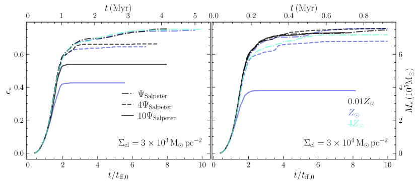
Figure 1: The star formation efficiency as a function of time for our simulations; $\Psi_{\mathrm{UV}}=1,4,\&10\,\Psi_{\mathrm{Fiducial}}$ are represented by dashdot, dashed, and solid lines respectively, colours indicate the different metallicities we explore, and the two panels represent the different $\Sigma_{\mathrm{cloud}}$ values in our simulation suite (Table 1). All our simulations undergo rapid collapse (over $t\lesssim 2t_{\mathrm{ff}}$) and star formation followed by a saturation in $\epsilon_{*}$ at the point when feedback is able to counteract the collapse; this saturation point is clearly different across our runs.

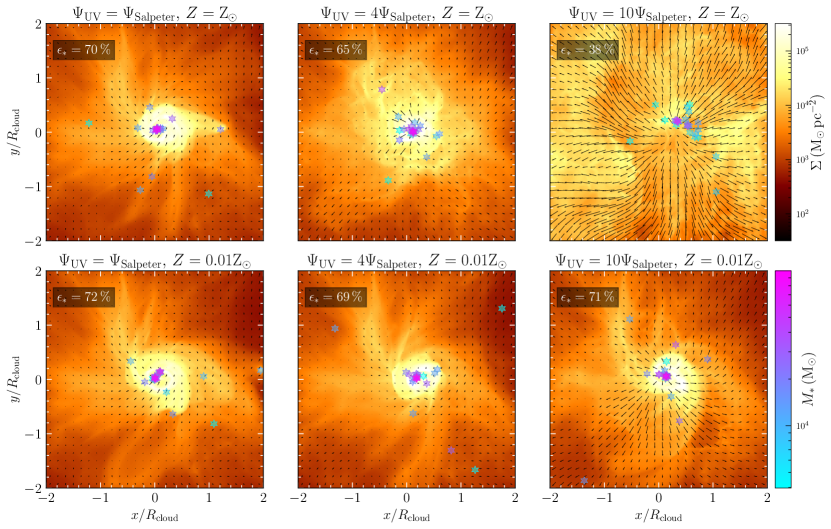
Figure 2: Gas surface density distributions at a time $t=4t_{\mathrm{ff}}$ for the $\Sigma_{\mathrm{cloud}}=3.2\times 10^{4}\,\,\mathrm{M}_{\sun}\,\mathrm{pc}^{-2}$ runs with increasing $\Psi_{\mathrm{UV}}$ (left to right) at $Z=Z_{\odot}$ (top) and $Z=0.01Z_{\odot}$ (bottom). We can see the general trend of a stronger impact of feedback at higher $\Psi_{\mathrm{UV}}$ and $Z$, as evidenced by presence/absence of outflows in the velocity distribution, which are driven by radiation pressure on dust. The star formation efficiency ($\epsilon_{*}$; annotated top-left of each panel) is high in all these cases, except when both $\Psi_{\mathrm{UV}}$ and $Z$ are high. Comparison of the achieved $\epsilon_{*}$ in the top-right and bottom-right panels demonstrate that a drop in $Z$ can counteract the effects of a higher $\Psi_{\mathrm{UV}}$.

3.2 Integrated Star formation efficiencies

The aforementioned trends are also reflected in the final saturated level of $\epsilon_{*}$ set by the star formation/feedback balance in our simulations – our key quantity of interest. We calculate this as the value at the point when there is less than $5\%$ of the gas mass remaining in the computational domain, and is indicated by the termination of the curves in Figure 1. When reporting this quantity we normalize by its corresponding value for a control run without any feedback to account for the initial gas mass loss due to our isolated turbulent cloud numerical setup, since this gas does not participate in the feedback-star formation competition; we refer to this normalised final star formation efficiency as $\epsilon_{*,\mathrm{f}}$. We also do this to place less emphasis on the exact value of $\epsilon_{*}$ in the simulation – since this is expected to vary depending on the turbulent initial conditions – but rather on the relative effect of the feedback for a given cloud. We show the values obtained for $\epsilon_{*,\mathrm{f}}$ across our simulation suite in Figure 3 as a function of the input value of $\Psi_{\mathrm{UV}}$ we use for the stellar populations. As expected, we can see the general trend that $\epsilon_{*,\mathrm{f}}$ decreases with increasing $\Psi_{\mathrm{UV}}$. However, $\epsilon_{*,\mathrm{f}}$ increases with decreasing $Z$ for a given $\Psi_{\mathrm{UV}}$. The dependence on $Z$ is weak for $\Sigma_{\mathrm{cloud}}\sim 10^{3}\,\,\mathrm{M}_{\sun}\,\mathrm{pc}^{-2}$ ($\lesssim 10\%$). However for the higher $\Sigma_{\mathrm{cloud}}$ case, the lower dust content can more or less completely counteract the effects of the higher $\Psi_{\mathrm{UV}}$. We can also see that $\epsilon_{*,\mathrm{f}}$ for the run with $Z\sim 4\mathrm{Z}_{\sun}$ is almost identical to the solar metallicity run; for the higher $\Sigma_{\mathrm{cloud}}$ case the difference is slightly more evident. This, along with the corresponding trends for lower metallicities, suggests that the dependence on dust content is stronger for the higher $\Sigma_{\mathrm{cloud}}$ case.

We also overplot approximate trends with $\Psi_{\mathrm{UV}}$ to guide the eye for $Z=\mathrm{Z}_{\sun}$ and $Z=0.01\mathrm{Z}_{\sun}$. We can see that the trend is largely linear (albeit with different slopes) for the lower $\Sigma_{\mathrm{cloud}}$ run, whereas it is clearly non-linear for the higher $\Sigma_{\mathrm{cloud}}$ at $Z=\mathrm{Z}_{\sun}$, but essentially flat for $Z=0.01\mathrm{Z}_{\sun}$. This implies that for this case, the lower dust-to-gas ratio completely compensates for the (high) increase in the UV luminosity. This has important implications for star cluster formation at high redshifts, as we will discuss below.

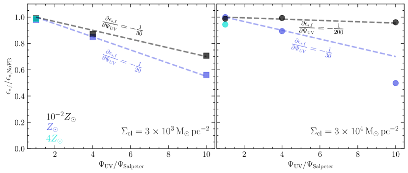
Figure 3: The final integrated cloud scale star formation efficiency ($\epsilon_{*,\mathrm{f}}$) obtained in all of our simulations – scaled by the value obtained for a run without feedback ($\epsilon_{*,\mathrm{NoFB}}$) – shown as a function of $\Psi_{\mathrm{UV}}$. We indicate lines and their slopes to guide the eye (no fitting). We can see that there is a general trend of decreasing $\epsilon_{*,\mathrm{f}}$ with $\Psi_{\mathrm{UV}}$, however, a lower $Z$ can at least partly compensate for this decrease – much more so for the higher $\Sigma_{\mathrm{cloud}}$ cases (right panel). The trend for the higher $\Sigma_{\mathrm{cloud}}$ case is also clearly non-linear. These trends are likely driven by the differing levels of momentum imparted by radiation pressure on dust across our simulations (see Section 3.3).

3.3 Physics driving trends

In this section we briefly explain the feedback physics that drives the trends with $\Psi_{\mathrm{UV}}$ and $Z$ in our simulations. The primary feedback mechanisms that drives the dynamics in our clouds is the radiation pressure on dust grains – both the single-scattering UV force, and the multiple-scattering force due to re-emitted IR radiation by warm dust. The former applies a constant force over the absorbing shell of $\sim L_{*}/c$ as long as it is optically thick in the UV; this requires $\Sigma\gtrsim 5(Z/\mathrm{Z}_{\sun})^{-1}\,\mathrm{M}_{\sun}\,\mathrm{pc}^{-2}$, which is satisfied across our parameter space even for the $Z=0.01\mathrm{Z}_{\sun}$ runs. On the other hand, to be optically thick in the IR requires $\Sigma\gtrsim 10^{3}(Z/\mathrm{Z}_{\sun})^{-1}\,\mathrm{M}_{\sun}\,\mathrm{pc}^{-2}$ assuming an average $\kappa_{\mathrm{IR}}=5\,\mathrm{cm}^{2}\,\mathrm{g}^{-1}$. Of the simulations we present in this paper, only the two with $\Sigma_{\mathrm{cloud}}\gtrsim 10^{4}\,\,\mathrm{M}_{\sun}\,\mathrm{pc}^{-2}$ with $Z=\mathrm{Z}_{\sun}$ and $4\mathrm{Z}_{\sun}$ satisfy this condition. These points imply that the IR radiation pressure is only an important contributor for these subset of runs – this is consistent with the findings reported in Menon et al. (2023). In these conditions, the trapped IR radiation field can impart a force $\sim f_{\mathrm{trap}}L_{*}/c$, where $f_{\mathrm{trap}}$ describes the trapping factor that quantifies the momentum gained by the multiple scattering of the IR radiation.

Now the competition between radiation pressure and gravity can be quantified with the Eddington ratio. The Eddington ratio for a column of gas with surface density $\Sigma$ exposed to a stellar population with UV luminosity-per unit mass $\Psi_{\mathrm{UV}}$ for single-scattering radiation pressure is (e.g., Thompson et al., 2015)

$$\Gamma_{\mathrm{UV}}=\frac{\Psi_{\mathrm{UV}}}{4\pi Gc\Sigma}\sim 0.1\left(\frac{\Psi_{\mathrm{UV}}}{\Psi_{\mathrm{Fiducial}}}\right)\left(\frac{\Sigma}{3000\,\mathrm{M}_{\odot}\,\mathrm{pc}^{-2}}\right)^{-1}.$$ (2)

Since there would be a distribution of $\Sigma$ surrounding the stellar population as the cloud evolves (Thompson & Krumholz, 2016), the above calculation suggests that the fraction of sightlines that become super-Eddington increases with $\Psi_{\mathrm{UV}}$. This could, to zeroth order, explain the trend we see in the $\Sigma_{\mathrm{cloud}}=3000\,\,\mathrm{M}_{\sun}\,\mathrm{pc}^{-2}$ runs. Note that there is no dependence on $Z$ for $\Gamma_{\mathrm{UV}}$, as long as the gas is optically thick in the UV.

On the other hand, for the multiple-scattering IR radiation force, the Eddington ratio is

$$\Gamma_{\mathrm{IR}}=\frac{\kappa_{\mathrm{IR}}\Psi_{\mathrm{UV}}}{4\pi Gc}=0.4\left(\frac{\kappa_{\mathrm{IR}}}{5\,\mathrm{cm}^{2}\,\mathrm{g}^{-1}}\right)\left(\frac{\Psi_{\mathrm{UV}}}{\Psi_{\mathrm{Fiducial}}}\right)\left(\frac{Z}{\mathrm{Z}_{\sun}}\right),$$ (3)

where we explicitly note the (assumed) linear dependence of $\kappa_{\mathrm{IR}}$ – the IR opacity – on the metallicity. Note that this does not have a dependence on $\Sigma$, as long as the column is optically thick in the IR, i.e. $\Sigma\gtrsim 10^{3}(Z/\mathrm{Z}_{\sun})^{-1}\,\mathrm{M}_{\sun}\,\mathrm{pc}^{-2}$.

We can now understand the stronger metallicity dependence for the higher $\Sigma_{\mathrm{cloud}}$ case: it is in the regime where the dust-to-gas ratio dependent IR radiation pressure is the dominant feedback mechanism. This force only plays a relatively minor role for $\Sigma_{\mathrm{cloud}}\lesssim 10^{4}\,\,\mathrm{M}_{\sun}\,\mathrm{pc}^{-2}$ – even less so at lower $Z$ – as it is optically thin in the IR. For the higher $\Sigma_{\mathrm{cloud}}$ case the IR radiation pressure is clearly the crucial force as the UV radiation pressure has insufficient momentum to compete with gravity at this high $\Sigma$ – even for $\Psi_{\mathrm{UV}}=10\Psi_{\mathrm{Fiducial}}$. This is reflected in the value of $\epsilon_{*,\mathrm{f}}$ for $Z=0.01\mathrm{Z}_{\sun}$ where only the UV acts; an inspection of Equation 2 clearly indicates sub-Eddington conditions for these parameters. The linear dependence on $\Psi_{\mathrm{UV}}$ in Equation 2 also explains the linear trend seen with $\Psi_{\mathrm{UV}}$ for the lower $\Sigma_{\mathrm{cloud}}$ cases. Finally, we find that the non-linear trend seen at $Z=\mathrm{Z}_{\sun}$ for the higher $\Sigma_{\mathrm{cloud}}$ runs is due to the subtle effect of more efficient trapping of IR photons – i.e. higher $f_{\mathrm{trap}}$ – for clouds with higher $\Psi_{\mathrm{UV}}$. This occurs because the (IR) radiation temperature is significantly higher for higher $\Psi_{\mathrm{UV}}$, which renders $\kappa_{\mathrm{IR}}$ higher, thereby imparting more momentum per unit stellar mass. Connecting with Equation 3, it is the combination of increasing $\kappa_{\mathrm{IR}}$ due to warmer dust along with the linear increase due to $\Psi_{\mathrm{UV}}$ that leads to the non-linear trend.

4 Discussion

4.1 Implications for massive galaxies at cosmic noon

Higher global star formation efficiencies than the local Universe and a top-heavy IMF are two of several proposed scenarios to reconcile the observed abundance of massive UV-bright galaxies at $z\sim 8$–$12$ with pre-launch model predictions (Inayoshi et al., 2022; Harikane et al., 2023; Finkelstein et al., 2023b; Yung et al., 2024). The former is a key element of the Feedback-Free Burst (FFB) model (Dekel et al., 2023), which invokes high cloud-scale SFE and ineffective feedback by stellar and supernova driven winds to achieve more efficient galaxy-scale star formation and hence boost the numbers of UV-luminous galaxies at early times. Li et al. (2023) showed that this model is consistent with observations when they adopt cloud-scale SFE of $\lesssim 50\%$. On the other hand, a top-heavy IMF and the associated higher UV luminosities could also match the UV luminosity functions while still adopting the lower SFEs that seem to be typical of galaxy populations at $z\lesssim 8$ (Tacchella et al., 2018); Yung et al. (2024) show that a boost of $\sim 4$ in the UV luminosity-to-mass ratio can reproduce the UV luminosity function at $z\sim 11$ without modifying the star formation efficiency or feedback strength. However, these studies explored the impact of the SFE and the IMF as if they were independent, which of course is not the case in reality. In this study, we have quantified how these two quantities depend on each other at the cloud scale.

Our results indicate that as long as clouds have surface densities $\Sigma_{\mathrm{cloud}}\gtrsim 10^{3}\,\,\mathrm{M}_{\sun}\,\mathrm{pc}^{-2}$ – a condition that seems to be commonly satisfied at $z\gtrsim 10$ based on observed galaxy sizes (e.g., Finkelstein et al., 2023b; Adamo et al., 2024; Casey et al., 2023; Morishita et al., 2023) – a star formation efficiency significantly higher than that typical of the Local Universe ($\sim 10\%$) is unavoidable even in the presence of a top-heavy IMF (we have investigated cases where the luminosity-to-mass ratio is up to ten times the typical value; see Figure 4 and Section A). A top-heavy IMF results in only a moderate reduction in the star formation efficiency, and only if the dust abundance is similar to the solar neighborhood. For metallicites that seem to be typical at the highest redshifts where we have reliable estimates, $z\sim 8$–10, i.e. $Z\sim 0.1$-0.3 $\mathrm{Z}_{\sun}$ (Curti et al., 2023; Nakajima et al., 2023), and assuming a linear relation between dust-to-gas ratio and metallicity, the SFE is higher for a given $\Psi_{\mathrm{UV}}$, and completely counteracts the effects of $\Psi_{\mathrm{UV}}$ for highly compact clouds ($\gtrsim 10^{4}\,\,\mathrm{M}_{\sun}\,\mathrm{pc}^{-2}$). Moreover, the nature of the IMF for conditions at $z\sim 10$ is highly uncertain, with works suggesting that it could even be bottom-heavy (e.g., Conroy & van Dokkum, 2012; Tanvir et al., 2022; Tanvir & Krumholz, 2024); that being said, these studies probe the IMF in a mass range ($\lesssim 1\mathrm{M}_{\sun}$) that does not contribute to $\Psi_{\mathrm{UV}}$. Even if this scenario were true for the high-mass end of the IMF, it would only imply that even more efficient star formation would be required, as $\Psi_{\mathrm{UV}}$ would be even lower than with a standard IMF. All of this suggests that highly efficient star formation at the cloud scales may be ubiquitous in high redshift galaxies, irrespective of the properties of the stellar populations that populate them.

If we take this at face value, it is possible that the combination of a top-heavy IMF in addition to efficient star formation could overpredict the UV luminosity functions, since they both contribute to an excess at the bright end. However, there are two key subtleties to point out in this context. Firstly, studies that found that a factor $\sim 4$ increase in $\Psi_{\mathrm{UV}}$ is sufficient to reproduce the observations do not account for any possible dust extinction (e.g., Yung et al., 2024). Secondly, the SFE values and trends we quantify in this study are at the cloud scale ($\lesssim 10\,\mathrm{pc}$), whereas the quantity relevant for the luminosity functions is the baryon efficiency ratio defined over the whole galaxy ($\epsilon_{*,\mathrm{gal}}$). For instance, Li et al. (2023) find that the FFB model fits the tentative JWST data for $\epsilon_{*,\mathrm{gal}}\sim 20\%$. This could either reflect the true SFE values within each star-forming cluster or alternatively reflect a duty cycle of star formation in the galaxy. The FFB scenario does predict a duty cycle, due to the need to accumulate enough accreted gas for triggering the fragmentation into star-forming clouds, which can lead to an $\epsilon_{*,\mathrm{gal}}\sim 20\%$ in spite of the assumed SFE $\sim 100\%$ at the scale of the individual clouds (Dekel et al., 2023; Li et al., 2023). The results obtained in the current work of higher SFE within the individual clusters is consistent with this duty-cycle interpretation of the lower SFE when averaged over time in the galaxy.

Alternatively, another possibility to reconcile our high cloud-scale SFE values with relatively lower $\epsilon_{*,\mathrm{gal}}$ is that only a fraction of the gas in the galaxy participates in star formation in clouds. It is possible the remaining gas is ejected in outflows by the feedback from older stellar populations, possibly explaining the dust-free nature of these galaxies (Fiore et al., 2023; Ferrara et al., 2023; Ferrara, 2023), which is likely critical to simultaneously explain the observed UV luminosity functions and the blue UV continuum slopes (e.g., Cullen et al., 2023) – although see Li et al. (2023) for an alternative explanation of these findings. This possibility raises another effect of a top-heavy IMF that we cannot capture in our simulations: a top-heavy IMF, would lead to more energy and mass loaded winds, potentially further decreasing $\epsilon_{*,\mathrm{gal}}$, such that its combination with a top-heavy IMF could be consistent with the observations. There is scope for studying the interaction of these three key parameters – SFE at the cloud scale, IMF, and the feedback effects in driving galaxy-scale winds, taking into account their respective dependencies on each other. By combining these joint constraints into a galaxy-scale semianalytic model (SAM; Somerville & Davé, 2015), we may be able to constrain the regions of parameter space permitted by the observations.

4.2 Missing physics and possible implications

It is important to note that several physical mechanisms are missing in our numerical simulations – we list them here and discuss how they might affect the outcomes.

We only model the radiative feedback on dust, and do not include photoionization and therefore the momentum from the associated thermal pressure of ionized gas. However, we argue that this would make little difference to the outcome of our simulations, as the clouds we model have escape speeds $v_{\mathrm{esc}}\gtrsim$ $\sim 2$–$5c_{s,\mathrm{ion}}$ where $c_{s,\mathrm{ion}}\sim 10\,\mathrm{km}\,\mathrm{s}^{-1}$ is the ionized gas sound speed. These arguments are consistent with results presented in models and previous numerical simulations that show that radiation pressure on dust is the dominant radiative feedback mechanism in this regime for regulating star formation (Krumholz & Matzner, 2009; Dale et al., 2012; Kim et al., 2016, 2018). We also demonstrate this is the case in Appendix B by re-running one of our models with the effects of photo-ionization included. We can justify the omission of protostellar outflows along similar lines – $v_{\mathrm{esc}}$ is much higher than the $\sim 1\,\mathrm{km}\,\mathrm{s}^{-1}$ threshold suggested by Matzner & Jumper (2015) for effective gas ejection by jets.

We also do not model stellar winds. While this might at first seem like a major omission, we note that the effectiveness of stellar wind feedback has been shown to be reduced compared to analytic estimates due to efficient cooling at turbulent interfaces in the multiphase gas, rendering it momentum-limited (Lancaster et al., 2021b, c); this has been shown to be especially true in the regime of high $\Sigma_{\mathrm{cloud}}\gtrsim 10^{3}\,\,\mathrm{M}_{\sun}\,\mathrm{pc}^{-2}$ (Lancaster et al., 2021a) that we focus on here. However, this still implies that there would be a force $\dot{p}_{\mathrm{w}}$ – where $\dot{p}_{\mathrm{w}}\sim\dot{M_{\mathrm{w}}}v_{\mathrm{w}}$ is the wind momentum for a mass-loss rate $\dot{M_{\mathrm{w}}}$ and wind-velocity $v_{\mathrm{w}}$ – acting on the gas. $\dot{p}_{\mathrm{w}}$ is expected to be $\sim L_{*}/c$ for a stellar population (see Figure 3, Lancaster et al., 2021b), suggesting that this should induce an order unity correction to our obtained values of $\epsilon_{*,\mathrm{f}}$. In other words, it is possible that the $\epsilon_{*,\mathrm{f}}$ obtained at $\Psi_{\mathrm{UV}}=10$ would be obtained for $\Psi_{\mathrm{UV}}=5$ with the additional effect of stellar winds. That being said, it is highly likely that the two feedback mechanisms do not interact in a simple additive fashion. Moreover, at metallicities $Z\lesssim 0.1\mathrm{Z}_{\sun}$ winds from massive O stars are considerably weaker (Leitherer et al., 1992; Vink et al., 2001), meaning that significant stellar wind feedback is delayed until the onset of Wolf-Rayet winds (Lancaster et al., 2021b; Dekel et al., 2023). This time delay may be too long to have a significant impact on star formation in clouds of these densities. Numerical simulations that combine wind and radiative feedback would provide more formal quantification of the resultant star formation efficiencies in such conditions.

We assume perfect coupling between gas and dust temperatures, and radiative equilibrium for the radiation and dust temperatures. These assumptions are quite reasonable when our clouds are optically thick in the IR; however, for our simulations with $Z\sim 0.01\mathrm{Z}_{\sun}$, they start to break down. For instance, dust and gas temperatures likely decouple in these conditions except in very high density regions ($n\gtrsim 10^{7}\mathrm{cm}^{-3}$), which renders our estimates for the gas temperatures incorrect. However, the dynamical impact of this would be minor, since the thermal pressure is not a significant force in the systems we are investigating. The fragmentation properties in our simulations would be affected by this error, but we do not resolve individual stars anyway and our scope is limited to studying the net competition between radiation forces and gravity in clouds, which is unlikely to be affected.

Our assumption that the dust and the radiation field are in LTE also starts to break down at low dust-to-gas ratios when the dust becomes optically thin in the IR. In this limit, the color temperature of the IR radiation field at any spatial location is not equal to the local dust temperature – an effect that can only be captured by a numerical method that models the evolution of the full SED through the cloud. The way in which this assumption directly affects our numerical model is that our estimated dust temperatures would be incorrect in the optically-thin limit, directly affecting the IR dust absorption opacities, which then subsequently affects the IR component of the radiation force (which is $\propto$ opacity). However, we estimate that the impact of this would be minor, since this error only applies in the limit where the dust is optically thin in the IR, in which case we are in the single scattering regime anyway and the IR radiation force is negligible; the latter becomes important only when optically thick in the IR, in which case our assumption is valid. One might question if the very statement that the cloud is optically thick/thin in the IR might itself be affected by the (indirect) error we make in the dust opacity. We estimate that this is unlikely since the range of (gray) IR opacities for dust warmer than 40 K varies by at most a factor $\sim$ few (see Figure 1; Menon et al., 2022a). Therefore even if we assume significant error in the dust temperature (which is itself unlikely), it results in the IR dust opacity being underestimated by a factor $\sim$ few, which is insufficient to alter the regime of the problem from the single scattering to the multiple scattering regime for our $Z=0.01\mathrm{Z}_{\sun}$ clouds, which are optically thin by at least 1-2 orders of magnitude. Hence, the impact of this assumption on our results are unlikely to be significant. That being said, this is a subtle effect that could affect systems that are marginally optically thick; there is scope for future (frequency-dependent) calculations to quantify the impact of this assumption in such conditions.

We also do not include magnetic fields which could provide additional support against gravitational collapse and therefore possibly render higher fractions of gas unbound (e.g., Burkhart, 2018; Krumholz & Federrath, 2019; Kim et al., 2021). In addition, we do not have the influence of an external larger-scale turbulent environment which could provide additional stabilization (Kim et al., 2021; Orr et al., 2022; Forbes et al., 2023) through a turbulent cascade acting on the scales of our clouds but also possibly additional compressive modes (Appel et al., 2023). Both of these could slightly affect our obtained values of $\epsilon_{*,\mathrm{f}}$. We therefore urge caution in interpreting the exact values of $\epsilon_{*,\mathrm{f}}$ we report. We emphasize our main takeaway is the trends we find with the IMF and dust content (metallicity).

5 Conclusions

We study the efficiency of star formation set by radiative feedback for assumed IMFs that are (increasingly) top-heavy and at different dust-to-gas ratios (or metallicity $Z$, assuming a linear relation between the two). We focus on massive, dense, compact clouds with initial gas surface densities $\Sigma_{\mathrm{cloud}}\gtrsim 10^{3}\,\,\mathrm{M}_{\sun}\,\mathrm{pc}^{-2}$, which are likely typical for galaxies that have been detected by JWST at $z\sim 10$. Past theoretical studies have shown that clouds in this regime are expected to exhibit very high star formation efficiencies (e.g., Lancaster et al., 2021a; Menon et al., 2023; Polak et al., 2023) for a standard UV luminosity-to-mass assuming a Chabrier (2005) IMF ($\Psi_{\mathrm{Fiducial}}$). We test the effects of increased feedback due to a top-heavy IMF on such clouds, by assuming different values of the UV luminosity-to-mass ratios ($\Psi_{\mathrm{UV}}$) – up to $10\Psi_{\mathrm{Fiducial}}$ – for the stellar populations forming in our simulations. We also explore the effects of sub- and super-solar metallicities to mimic different environments/redshift conditions (see Table 1). Our takeaway findings are:

1. Efficient Star Formation: The integrated cloud-scale star formation efficiency ($\epsilon_{*,\mathrm{f}}$) is $\gtrsim 40\%$ in all our simulations in spite of very top-heavy IMFs. This is much higher than that typical of young star clusters in the Local Universe ($\epsilon_{*,\mathrm{f}}\lesssim 10\%$), suggesting that (relatively) efficient star formation is unavoidable at high gas/stellar surface densities.

2. Effects of Top-Heavy IMF: Efficiencies are lower for an increasingly top-heavy IMF (i.e., higher $\Psi_{\mathrm{UV}}$). We find that for solar-neighborhood dust conditions, $\epsilon_{*,\mathrm{f}}$ decreases with $\Psi_{\mathrm{UV}}$ by up to $50\%$ ($20\%$) for an increase in $\Psi_{\mathrm{UV}}$ by a factor 10 (4).

3. Effects of Dust-to-Gas Ratio: Efficiencies are higher for sub-solar metallicity/dust abundance, which seems to at least partly compensate for the effects of a top-heavy IMF (Figure 3). This effect is much stronger for more compact clouds ($\Sigma_{\mathrm{cloud}}\gtrsim 10^{4}\,\,\mathrm{M}_{\sun}\,\mathrm{pc}^{-2}$) such that the star formation efficiency is indistinguishable from the fiducial case even at $\Psi_{\mathrm{UV}}=10\Psi_{\mathrm{Fiducial}}$. At $\Sigma_{\mathrm{cloud}}\sim 10^{3}\,\,\mathrm{M}_{\sun}\,\mathrm{pc}^{-2}$ the effect of the dust content are more modest ($\lesssim 10\%$).

4. Radiative Feedback: We find that our trends can be explained by the impact of $\Psi_{\mathrm{UV}}$ and $Z$ on the momentum from radiation pressure on dust (Section 3.3). Higher $\Psi_{\mathrm{UV}}$ leads to higher momentum per-unit stellar mass, whereas lower dust abundances ($Z$) reduces the important additional contribution from the dust-reprocessed infrared radiation pressure.

Appendix A UV Luminosity of Stellar Populations

In this appendix we present calculations of the UV output of stellar populations using the Stochastically Lighting Up Galaxies (SLUG; da Silva et al., 2012; Krumholz et al., 2015) stellar population synthesis code. We compute models of star cluster masses $M=M_{\mathrm{cloud}}=10^{6}\,\mathrm{M}_{\sun}$ with increasingly top-heavy IMF prescriptions to motivate the parameter space of $\Psi$ we explore in our simulations. We use a Chabrier (2005) functional form for the IMF of the stellar population with values for the mean and standard deviation of the lognormal part of the IMF ($M<1\mathrm{M}_{\sun}$) as $0.2\mathrm{M}_{\sun}$ and 0.55 dex, and a power law for $M>1\mathrm{M}_{\sun}$ with slope $\alpha$, where $\alpha=-2.35$ is the value consistent with the Salpeter (1955) IMF; the transition from the lognormal to the power-law occurs at $M=1\mathrm{M}_{\sun}$. We mimic a top-heavy IMF in two independent ways to test its impact on the UV luminosity of the stellar population – i) changing the high-mass slope $\alpha$ while keeping the other parameters and functional forms the same, and ii) changing the upper limit of the stellar mass range of the IMF ($M_{\mathrm{max}}$) while fixing $\alpha=-2.35$, where $120\mathrm{M}_{\sun}$ is the value for the standard fiducial IMF. We note that there are several other ways to achieve a top-heavy IMF, such as changing the peak of the IMF and/or the functional form itself, as predicted by several models (e.g., Sharda & Krumholz, 2022). However, our intention with this calculation is simply to provide the reader a sense of the mapping between the IMF and the UV luminosities of the stellar populations.

We explore values of $-2.5\leq\alpha\leq-1$ and $80\mathrm{M}_{\sun}\leq M_{\mathrm{max}}\leq 300$. All our models use the MIST v1.0 isochrones (Choi et al., 2016) rotating at $40\%$ breakup, Solar metallicity, and SLUG’s Starburst99 option for stellar atmospheres, which follows the approach described by Leitherer et al. (1999) and implemented in the Starburst99 stellar population synthesis code. We evolve our star cluster model for 5 Myr, and then compute the time-averaged UV ($h\nu\geq 6.6\,\mathrm{eV}$) bolometric luminosity ($L_{\mathrm{UV}}$); the luminosities are relatively constant over this timescale after which it significantly drops due to the death of massive stars. In Figure 4 we report these values in units of the corresponding estimate for the Salpeter 1955 slope $\alpha=-2.35$ and $M_{\mathrm{max}}=120\mathrm{M}_{\sun}$.

Figure 4: The UV luminosity per-unit mass of stars: i) for a given slope at the high-mass end of the IMF ($\alpha$; left panel), and ii) for a fixed Salpeter slope but different upper stellar mass limits ($M_{\mathrm{max}}$), both normalised by its counterpart for a standard Chabrier IMF – i.e. a Salpeter slope (i.e. $\alpha=-2.35$) and an upper mass limit of 120$\mathrm{M}_{\sun}$. These values have been obtained with the SLUG stellar population synthesis code. The peak mass of the IMF and its shape are kept identical in this calculation – only the high-mass slope and the upper mass limit are varied independently. We use this range of values ($\Psi_{\mathrm{UV}}\sim 1$–$10\,\Psi_{\mathrm{Salpeter}}$) to motivate the parameter space we explore.

Appendix B Impact of Photoionization

The simulations presented in this study do not include the photoionization of hydrogen, and the associated thermal pressure of photoionized gas that could act to regulate star formation. We argued that this omission does not impact our outcomes as the dynamical impact of the thermal pressure of photoionized gas is expected to be minor for these clouds with high escape velocities. We demonstrate this is the case by recomputing our metal-poor, highly top-heavy run (i.e. $Z=10^{-2}Z_{\odot}$, $\Psi_{\mathrm{UV}}=10\Psi_{\mathrm{Salpeter}}$) for $\Sigma_{\mathrm{cloud}}=3\times 10^{4}\,\,\mathrm{M}_{\sun}\,\mathrm{pc}^{-2}$ with photoionization included. Our final normalized star formation efficiency $\epsilon_{*,\mathrm{f}}/\epsilon_{*,\mathrm{NoFB}}$ with and without photoionization are 92% and 97% respectively. This confirms that photoionization plays a very minor role in this regime, and thereby its omission does not affect our results.

For completeness, we describe the additional parameters used for including the LyC band. We use the radiative luminosities for this run consistent with the values reported in Figure 4 for $\Psi_{\mathrm{UV}}=10$. We use a cross section to ionizing photons for hydrogen corresponding to the Lyman edge $\sigma_{ion}=6.3\times 10^{-18}\,\mathrm{cm}^{2}$, and a constant (case-B) recombination coefficient $\alpha_{\mathrm{B}}=2.6\times 10^{-13}\,\mathrm{cm}^{3}\,\mathrm{s}^{-1}$. For simplicity, we also assume instantaneous thermal equilibrium for the ionized/neutral phases, by setting the temperature proportional to the ionization fraction such that fully ionized (neutral) gas has a temperature of $10^{4}\,\mathrm{K}$ ($10\,\mathrm{K}$) – i.e. the two-temperature isothermal equation of state (e.g., Gritschneder et al., 2009; Kim et al., 2018; Menon et al., 2020). We also include the associated radiation pressure on gas due to LyC absorption.

References

- Adamo et al. (2024) Adamo, A., Bradley, L. D., Vanzella, E., et al. 2024, arXiv e-prints, arXiv:2401.03224, doi: 10.48550/arXiv.2401.03224
- Appel et al. (2022) Appel, S. M., Burkhart, B., Semenov, V. A., Federrath, C., & Rosen, A. L. 2022, ApJ, 927, 75, doi: 10.3847/1538-4357/ac4be3
- Appel et al. (2023) Appel, S. M., Burkhart, B., Semenov, V. A., et al. 2023, ApJ, 954, 93, doi: 10.3847/1538-4357/ace897
- Balay et al. (1997) Balay, S., Gropp, W. D., McInnes, L. C., & Smith, B. F. 1997, in Modern Software Tools in Scientific Computing, ed. E. Arge, A. M. Bruaset, & H. P. Langtangen (Birkhäuser Press), 163–202
- Balay et al. (2021) Balay, S., Abhyankar, S., Adams, M. F., et al. 2021, PETSc/TAO Users Manual, Tech. Rep. ANL-21/39 - Revision 3.16, Argonne National Laboratory
- Buntemeyer et al. (2016) Buntemeyer, L., Banerjee, R., Peters, T., Klassen, M., & Pudritz, R. E. 2016, New Astronomy, 43, 49, doi: 10.1016/j.newast.2015.07.002
- Burkhart (2018) Burkhart, B. 2018, ApJ, 863, 118, doi: 10.3847/1538-4357/aad002
- Burkhart et al. (2024) Burkhart, B., Bialy, S., Seifried, D., et al. 2024, arXiv e-prints, arXiv:2402.01587, doi: 10.48550/arXiv.2402.01587
- Casey et al. (2014) Casey, C. M., Narayanan, D., & Cooray, A. 2014, Phys. Rep., 541, 45, doi: 10.1016/j.physrep.2014.02.009
- Casey et al. (2023) Casey, C. M., Akins, H. B., Shuntov, M., et al. 2023, arXiv e-prints, arXiv:2308.10932, doi: 10.48550/arXiv.2308.10932
- Chabrier (2005) Chabrier, G. 2005, in Astrophysics and Space Science Library, Vol. 327, The Initial Mass Function 50 Years Later, ed. E. Corbelli, F. Palla, & H. Zinnecker, 41
- Chevance et al. (2023) Chevance, M., Krumholz, M. R., McLeod, A. F., et al. 2023, in Astronomical Society of the Pacific Conference Series, Vol. 534, Protostars and Planets VII, ed. S. Inutsuka, Y. Aikawa, T. Muto, K. Tomida, & M. Tamura, 1, doi: 10.48550/arXiv.2203.09570
- Choban et al. (2022) Choban, C. R., Kereš, D., Hopkins, P. F., et al. 2022, MNRAS, 514, 4506, doi: 10.1093/mnras/stac1542
- Choi et al. (2016) Choi, J., Dotter, A., Conroy, C., et al. 2016, ApJ, 823, 102, doi: 10.3847/0004-637X/823/2/102
- Chon et al. (2023) Chon, S., Hosokawa, T., Omukai, K., & Schneider, R. 2023, arXiv e-prints, arXiv:2312.13339, doi: 10.48550/arXiv.2312.13339
- Chon et al. (2022) Chon, S., Ono, H., Omukai, K., & Schneider, R. 2022, MNRAS, 514, 4639, doi: 10.1093/mnras/stac1549
- Conroy & van Dokkum (2012) Conroy, C., & van Dokkum, P. G. 2012, ApJ, 760, 71, doi: 10.1088/0004-637X/760/1/71
- Costa et al. (2021) Costa, A. H., Johnson, K. E., Indebetouw, R., et al. 2021, ApJ, 918, 76, doi: 10.3847/1538-4357/ac0e93
- Cullen et al. (2023) Cullen, F., McLeod, D. J., McLure, R. J., et al. 2023, arXiv e-prints, arXiv:2311.06209, doi: 10.48550/arXiv.2311.06209
- Curti et al. (2023) Curti, M., Maiolino, R., Curtis-Lake, E., et al. 2023, arXiv e-prints, arXiv:2304.08516, doi: 10.48550/arXiv.2304.08516
- da Silva et al. (2012) da Silva, R. L., Fumagalli, M., & Krumholz, M. 2012, ApJ, 745, 145, doi: 10.1088/0004-637X/745/2/145
- Dale et al. (2012) Dale, J. E., Ercolano, B., & Bonnell, I. A. 2012, MNRAS, 424, 377, doi: 10.1111/j.1365-2966.2012.21205.x
- Dayal et al. (2017) Dayal, P., Choudhury, T. R., Bromm, V., & Pacucci, F. 2017, ApJ, 836, 16. https://arxiv.org/abs/1501.02823
- De Vis et al. (2019) De Vis, P., Jones, A., Viaene, S., et al. 2019, A&A, 623, A5, doi: 10.1051/0004-6361/201834444
- Dekel et al. (2023) Dekel, A., Sarkar, K. C., Birnboim, Y., Mandelker, N., & Li, Z. 2023, MNRAS, 523, 3201, doi: 10.1093/mnras/stad1557
- Diamond-Stanic et al. (2012) Diamond-Stanic, A. M., Moustakas, J., Tremonti, C. A., et al. 2012, ApJ, 755, L26, doi: 10.1088/2041-8205/755/2/L26
- Draine (2011) Draine, B. T. 2011, ApJ, 732, 100, doi: 10.1088/0004-637X/732/2/100
- Dubey et al. (2008) Dubey, A., Reid, L. B., & Fisher, R. 2008, Physica Scripta Volume T, 132, 014046, doi: 10.1088/0031-8949/2008/T132/014046
- Emig et al. (2020) Emig, K. L., Bolatto, A. D., Leroy, A. K., et al. 2020, ApJ, 903, 50, doi: 10.3847/1538-4357/abb67d
- Fall et al. (2010) Fall, S. M., Krumholz, M. R., & Matzner, C. D. 2010, Astrophysical Journal Letters, 710, L142, doi: 10.1088/2041-8205/710/2/L142
- Federrath et al. (2010a) Federrath, C., Banerjee, R., Clark, P. C., & Klessen, R. S. 2010a, ApJ, 713, 269, doi: 10.1088/0004-637X/713/1/269
- Federrath et al. (2011) Federrath, C., Banerjee, R., Seifried, D., Clark, P. C., & Klessen, R. S. 2011, in IAU Symposium, Vol. 270, Computational Star Formation, ed. J. Alves, B. G. Elmegreen, J. M. Girart, & V. Trimble, 425–428, doi: 10.1017/S1743921311000755
- Federrath et al. (2010b) Federrath, C., Roman-Duval, J., Klessen, R. S., Schmidt, W., & Mac Low, M. M. 2010b, A&A, 512, A81, doi: 10.1051/0004-6361/200912437
- Federrath et al. (2022) —. 2022, TG: Turbulence Generator, Astrophysics Source Code Library, record ascl:2204.001. http://ascl.net/2204.001
- Feldmann (2015) Feldmann, R. 2015, MNRAS, 449, 3274, doi: 10.1093/mnras/stv552
- Ferrara (2023) Ferrara, A. 2023, arXiv e-prints, arXiv:2310.12197, doi: 10.48550/arXiv.2310.12197
- Ferrara et al. (2023) Ferrara, A., Pallottini, A., & Dayal, P. 2023, MNRAS, 522, 3986, doi: 10.1093/mnras/stad1095
- Finkelstein et al. (2023a) Finkelstein, S. L., Bagley, M. B., Ferguson, H. C., et al. 2023a, ApJ, 946, L13, doi: 10.3847/2041-8213/acade4
- Finkelstein et al. (2023b) Finkelstein, S. L., Leung, G. C. K., Bagley, M. B., et al. 2023b, arXiv e-prints, arXiv:2311.04279, doi: 10.48550/arXiv.2311.04279
- Finn et al. (2019) Finn, M. K., Johnson, K. E., Brogan, C. L., et al. 2019, ApJ, 874, 120, doi: 10.3847/1538-4357/ab0d1e
- Fiore et al. (2023) Fiore, F., Ferrara, A., Bischetti, M., Feruglio, C., & Travascio, A. 2023, ApJ, 943, L27, doi: 10.3847/2041-8213/acb5f2
- Forbes et al. (2023) Forbes, J. C., Emami, R., Somerville, R. S., et al. 2023, ApJ, 948, 107, doi: 10.3847/1538-4357/acb53e
- Fryxell et al. (2000) Fryxell, B., Olson, K., Ricker, P., et al. 2000, ApJS, 131, 273, doi: 10.1086/317361
- Fukushima & Yajima (2021) Fukushima, H., & Yajima, H. 2021, MNRAS, 506, 5512, doi: 10.1093/mnras/stab2099
- Fukushima & Yajima (2023) —. 2023, MNRAS, 524, 1422, doi: 10.1093/mnras/stad1956
- Gallegos-Garcia et al. (2020) Gallegos-Garcia, M., Burkhart, B., Rosen, A. L., Naiman, J. P., & Ramirez-Ruiz, E. 2020, ApJ, 899, L30, doi: 10.3847/2041-8213/ababae
- Geen et al. (2016) Geen, S., Hennebelle, P., Tremblin, P., & Rosdahl, J. 2016, MNRAS, 463, 3129, doi: 10.1093/mnras/stw2235
- Gritschneder et al. (2009) Gritschneder, M., Naab, T., Walch, S., Burkert, A., & Heitsch, F. 2009, Astrophysical Journal, 694, doi: 10.1088/0004-637X/694/1/L26
- Grudić et al. (2022) Grudić, M. Y., Guszejnov, D., Offner, S. S. R., et al. 2022, MNRAS, 512, 216, doi: 10.1093/mnras/stac526
- Grudić et al. (2018) Grudić, M. Y., Hopkins, P. F., Faucher-Giguère, C.-A., et al. 2018, MNRAS, 475, 3511, doi: 10.1093/mnras/sty035
- Harikane et al. (2023) Harikane, Y., Ouchi, M., Oguri, M., et al. 2023, ApJS, 265, 5, doi: 10.3847/1538-4365/acaaa9
- Harris et al. (2020) Harris, C. R., Millman, K. J., van der Walt, S. J., et al. 2020, Nature, 585, 357, doi: 10.1038/s41586-020-2649-2
- Hassan et al. (2023) Hassan, S., Lovell, C. C., Madau, P., et al. 2023, ApJ, 958, L3, doi: 10.3847/2041-8213/ad0239
- He et al. (2019) He, C.-C., Ricotti, M., & Geen, S. 2019, MNRAS, 489, 1880, doi: 10.1093/mnras/stz2239
- He et al. (2022) He, H., Wilson, C., Brunetti, N., et al. 2022, ApJ, 928, 57, doi: 10.3847/1538-4357/ac5628
- Hunter (2007) Hunter, J. D. 2007, Computing in Science Engineering, 9, 90, doi: 10.1109/MCSE.2007.55
- Inami et al. (2022) Inami, H., Surace, J., Armus, L., et al. 2022, ApJ, 940, L6, doi: 10.3847/2041-8213/ac9389
- Inayoshi et al. (2022) Inayoshi, K., Harikane, Y., Inoue, A. K., Li, W., & Ho, L. C. 2022, ApJ, 938, L10, doi: 10.3847/2041-8213/ac9310
- Jeffreson et al. (2024) Jeffreson, S. M. R., Semenov, V. A., & Krumholz, M. R. 2024, MNRAS, 527, 7093, doi: 10.1093/mnras/stad3550
- Johnson et al. (2015) Johnson, K. E., Leroy, A. K., Indebetouw, R., et al. 2015, ApJ, 806, 35, doi: 10.1088/0004-637X/806/1/35
- Kannan et al. (2022) Kannan, R., Garaldi, E., Smith, A., et al. 2022, MNRAS, 511, 4005, doi: 10.1093/mnras/stab3710
- Kannan et al. (2022) Kannan, R., Springel, V., Hernquist, L., et al. 2022, arXiv e-prints, arXiv:2210.10066. https://arxiv.org/abs/2210.10066
- Kim et al. (2023) Kim, J.-G., Gong, M., Kim, C.-G., & Ostriker, E. C. 2023, ApJS, 264, 10, doi: 10.3847/1538-4365/ac9b1d
- Kim et al. (2016) Kim, J.-G., Kim, W.-T., & Ostriker, E. C. 2016, ApJ, 819, 137, doi: 10.3847/0004-637X/819/2/137
- Kim et al. (2018) —. 2018, ApJ, 859, 68, doi: 10.3847/1538-4357/aabe27
- Kim et al. (2017) Kim, J.-G., Kim, W.-T., Ostriker, E. C., & Skinner, M. A. 2017, ApJ, 851, 93, doi: 10.3847/1538-4357/aa9b80
- Kim et al. (2021) Kim, J.-G., Ostriker, E. C., & Filippova, N. 2021, ApJ, 911, 128, doi: 10.3847/1538-4357/abe934
- Klessen & Glover (2023) Klessen, R. S., & Glover, S. C. O. 2023, ARA&A, 61, 65, doi: 10.1146/annurev-astro-071221-053453
- Krumholz & Federrath (2019) Krumholz, M. R., & Federrath, C. 2019, Frontiers in Astronomy and Space Sciences, 6, 7, doi: 10.3389/fspas.2019.00007
- Krumholz et al. (2015) Krumholz, M. R., Fumagalli, M., da Silva, R. L., Rendahl, T., & Parra, J. 2015, MNRAS, 452, 1447, doi: 10.1093/mnras/stv1374
- Krumholz et al. (2007) Krumholz, M. R., Klein, R. I., McKee, C. F., & Bolstad, J. 2007, ApJ, 667, 626, doi: 10.1086/520791
- Krumholz & Matzner (2009) Krumholz, M. R., & Matzner, C. D. 2009, Astrophysical Journal, 703, 1352, doi: 10.1088/0004-637X/703/2/1352
- Krumholz et al. (2006) Krumholz, M. R., Matzner, C. D., & McKee, C. F. 2006, ApJ, 653, 361, doi: 10.1086/508679
- Krumholz & Thompson (2012) Krumholz, M. R., & Thompson, T. A. 2012, ApJ, 760, 155, doi: 10.1088/0004-637X/760/2/155
- Lancaster et al. (2021a) Lancaster, L., Ostriker, E. C., Kim, J.-G., & Kim, C.-G. 2021a, ApJ, 922, L3, doi: 10.3847/2041-8213/ac3333
- Lancaster et al. (2021b) —. 2021b, ApJ, 914, 89, doi: 10.3847/1538-4357/abf8ab
- Lancaster et al. (2021c) —. 2021c, ApJ, 914, 90, doi: 10.3847/1538-4357/abf8ac
- Larson (1998) Larson, R. B. 1998, MNRAS, 301, 569, doi: 10.1046/j.1365-8711.1998.02045.x
- Leitherer et al. (1992) Leitherer, C., Robert, C., & Drissen, L. 1992, ApJ, 401, 596, doi: 10.1086/172089
- Leitherer et al. (1999) Leitherer, C., Schaerer, D., Goldader, J. D., et al. 1999, ApJS, 123, 3, doi: 10.1086/313233
- Leroy et al. (2018) Leroy, A. K., Bolatto, A. D., Ostriker, E. C., et al. 2018, The Astrophysical Journal, 869, 126, doi: 10.3847/1538-4357/aaecd1
- Levy et al. (2021) Levy, R. C., Bolatto, A. D., Leroy, A. K., et al. 2021, ApJ, 912, 4, doi: 10.3847/1538-4357/abec84
- Li et al. (2023) Li, Z., Dekel, A., Sarkar, K. C., et al. 2023, arXiv e-prints, arXiv:2311.14662, doi: 10.48550/arXiv.2311.14662
- Mac Low & Klessen (2004) Mac Low, M.-M., & Klessen, R. S. 2004, Reviews of Modern Physics, 76, 125, doi: 10.1103/RevModPhys.76.125
- Marshak (1958) Marshak, R. E. 1958, Physics of Fluids, 1, 24, doi: 10.1063/1.1724332
- Matzner & Jumper (2015) Matzner, C. D., & Jumper, P. H. 2015, ApJ, 815, 68, doi: 10.1088/0004-637X/815/1/68
- McCrady et al. (2005) McCrady, N., Graham, J. R., & Vacca, W. D. 2005, ApJ, 621, 278, doi: 10.1086/427487
- McKinney et al. (2023) McKinney, J., Pope, A., Kirkpatrick, A., et al. 2023, ApJ, 955, 136, doi: 10.3847/1538-4357/ace25c
- McLeod et al. (2024) McLeod, D. J., Donnan, C. T., McLure, R. J., et al. 2024, MNRAS, 527, 5004, doi: 10.1093/mnras/stad3471
- Menon et al. (2021) Menon, S. H., Federrath, C., Klaassen, P., Kuiper, R., & Reiter, M. 2021, MNRAS, 500, 1721, doi: 10.1093/mnras/staa3271
- Menon et al. (2022a) Menon, S. H., Federrath, C., & Krumholz, M. R. 2022a, MNRAS, 517, 1313, doi: 10.1093/mnras/stac2702
- Menon et al. (2023) —. 2023, MNRAS, 521, 5160, doi: 10.1093/mnras/stad856
- Menon et al. (2022b) Menon, S. H., Federrath, C., Krumholz, M. R., et al. 2022b, MNRAS, 512, 401, doi: 10.1093/mnras/stac485
- Menon et al. (2020) Menon, S. H., Federrath, C., & Kuiper, R. 2020, MNRAS, 493, 4643, doi: 10.1093/mnras/staa580
- Mihalas & Klein (1982) Mihalas, D., & Klein, R. I. 1982, Journal of Computational Physics, 46, 97, doi: 10.1016/0021-9991(82)90007-9
- Morishita et al. (2023) Morishita, T., Stiavelli, M., Chary, R.-R., et al. 2023, arXiv e-prints, arXiv:2308.05018, doi: 10.48550/arXiv.2308.05018
- Mowla et al. (2024) Mowla, L., Iyer, K., Asada, Y., et al. 2024, arXiv e-prints, arXiv:2402.08696, doi: 10.48550/arXiv.2402.08696
- Nakajima et al. (2023) Nakajima, K., Ouchi, M., Isobe, Y., et al. 2023, ApJS, 269, 33, doi: 10.3847/1538-4365/acd556
- Ochsendorf et al. (2017) Ochsendorf, B. B., Zinnecker, H., Nayak, O., et al. 2017, Nature Astronomy, 1, 784, doi: 10.1038/s41550-017-0268-0
- Oey et al. (2017) Oey, M. S., Herrera, C. N., Silich, S., et al. 2017, ApJ, 849, L1, doi: 10.3847/2041-8213/aa9215
- Omukai et al. (2005) Omukai, K., Tsuribe, T., Schneider, R., & Ferrara, A. 2005, ApJ, 626, 627, doi: 10.1086/429955
- Orr et al. (2022) Orr, M. E., Fielding, D. B., Hayward, C. C., & Burkhart, B. 2022, ApJ, 932, 88, doi: 10.3847/1538-4357/ac6c26
- Pascale et al. (2023) Pascale, M., Dai, L., McKee, C. F., & Tsang, B. T. H. 2023, ApJ, 957, 77, doi: 10.3847/1538-4357/acf75c
- Polak et al. (2023) Polak, B., Mac Low, M.-M., Klessen, R. S., et al. 2023, arXiv e-prints, arXiv:2312.06509, doi: 10.48550/arXiv.2312.06509
- Portegies Zwart et al. (2010) Portegies Zwart, S., McMillan, S., & Gieles, M. 2010, Annual Review of Astronomy and Astrophysics, 48, 431, doi: 10.1146/annurev-astro-081309-130834
- Raskutti et al. (2016) Raskutti, S., Ostriker, E. C., & Skinner, M. A. 2016, ApJ, 829, 130, doi: 10.3847/0004-637X/829/2/130
- Rémy-Ruyer et al. (2014) Rémy-Ruyer, A., Madden, S. C., Galliano, F., et al. 2014, A&A, 563, A31, doi: 10.1051/0004-6361/201322803
- Ricker (2008) Ricker, P. M. 2008, ApJS, 176, 293, doi: 10.1086/526425
- Rico-Villas et al. (2020) Rico-Villas, F., Martín-Pintado, J., González-Alfonso, E., Martín, S., & Rivilla, V. M. 2020, MNRAS, 491, 4573, doi: 10.1093/mnras/stz3347
- Robertson et al. (2023) Robertson, B., Johnson, B. D., Tacchella, S., et al. 2023, arXiv e-prints, arXiv:2312.10033, doi: 10.48550/arXiv.2312.10033
- Rupke et al. (2019) Rupke, D. S. N., Coil, A., Geach, J. E., et al. 2019, Nature, 574, 643, doi: 10.1038/s41586-019-1686-1
- Salpeter (1955) Salpeter, E. E. 1955, ApJ, 121, 161, doi: 10.1086/145971
- Schneider et al. (2018) Schneider, F. R. N., Sana, H., Evans, C. J., et al. 2018, Science, 359, 69, doi: 10.1126/science.aan0106
- Semenov et al. (2003) Semenov, D., Henning, T., Helling, C., Ilgner, M., & Sedlmayr, E. 2003, A&A, 410, 611, doi: 10.1051/0004-6361:20031279
- Sharda et al. (2023) Sharda, P., Amarsi, A. M., Grasha, K., et al. 2023, MNRAS, 518, 3985, doi: 10.1093/mnras/stac3315
- Sharda & Krumholz (2022) Sharda, P., & Krumholz, M. R. 2022, MNRAS, 509, 1959, doi: 10.1093/mnras/stab2921
- Skinner & Ostriker (2013) Skinner, M. A., & Ostriker, E. C. 2013, Astrophysical Journal, Supplement Series, 206, doi: 10.1088/0067-0049/206/2/21
- Smith et al. (2020) Smith, L. J., Bajaj, V., Ryon, J., & Sabbi, E. 2020, ApJ, 896, 84, doi: 10.3847/1538-4357/ab8f94
- Somerville & Davé (2015) Somerville, R. S., & Davé, R. 2015, ARA&A, 53, 51, doi: 10.1146/annurev-astro-082812-140951
- Sommovigo et al. (2022) Sommovigo, L., Ferrara, A., Pallottini, A., et al. 2022, MNRAS, 513, 3122, doi: 10.1093/mnras/stac302
- Sun et al. (2023) Sun, G., Faucher-Giguère, C.-A., Hayward, C. C., et al. 2023, ApJ, 955, L35, doi: 10.3847/2041-8213/acf85a
- Sun et al. (2024) Sun, J., He, H., Batschkun, K., et al. 2024, arXiv e-prints, arXiv:2401.14453. https://arxiv.org/abs/2401.14453
- Tacchella et al. (2018) Tacchella, S., Bose, S., Conroy, C., Eisenstein, D. J., & Johnson, B. D. 2018, ApJ, 868, 92, doi: 10.3847/1538-4357/aae8e0
- Tanvir & Krumholz (2024) Tanvir, T. S., & Krumholz, M. R. 2024, MNRAS, 527, 7306, doi: 10.1093/mnras/stad3581
- Tanvir et al. (2022) Tanvir, T. S., Krumholz, M. R., & Federrath, C. 2022, MNRAS, 516, 5712, doi: 10.1093/mnras/stac2642
- Thompson et al. (2015) Thompson, T. A., Fabian, A. C., Quataert, E., & Murray, N. 2015, MNRAS, 449, 147, doi: 10.1093/mnras/stv246
- Thompson & Krumholz (2016) Thompson, T. A., & Krumholz, M. R. 2016, Monthly Notices of the Royal Astronomical Society, 455, 334, doi: 10.1093/mnras/stv2331
- Turk et al. (2010) Turk, M. J., Smith, B. D., Oishi, J. S., et al. 2010, The Astrophysical Journal Supplement Series, 192, 9, doi: 10.1088/0067-0049/192/1/9
- Turner et al. (2015) Turner, J. L., Beck, S. C., Benford, D. J., et al. 2015, Nature, 519, 331, doi: 10.1038/nature14218
- Turner et al. (2017) Turner, J. L., Consiglio, S. M., Beck, S. C., et al. 2017, ApJ, 846, 73, doi: 10.3847/1538-4357/aa8669
- Upadhyaya et al. (2024) Upadhyaya, A., Marques-Chaves, R., Schaerer, D., et al. 2024, arXiv e-prints, arXiv:2401.16165, doi: 10.48550/arXiv.2401.16165
- Vanzella et al. (2022a) Vanzella, E., Castellano, M., Bergamini, P., et al. 2022a, A&A, 659, A2, doi: 10.1051/0004-6361/202141590
- Vanzella et al. (2022b) —. 2022b, ApJ, 940, L53, doi: 10.3847/2041-8213/ac8c2d
- Vink et al. (2001) Vink, J. S., de Koter, A., & Lamers, H. J. G. L. M. 2001, A&A, 369, 574, doi: 10.1051/0004-6361:20010127
- Virtanen et al. (2020) Virtanen, P., Gommers, R., Oliphant, T. E., et al. 2020, Nature Methods, 17, 261, doi: 10.1038/s41592-019-0686-2
- Waagan et al. (2011) Waagan, K., Federrath, C., & Klingenberg, C. 2011, Journal of Computational Physics, 230, 3331, doi: 10.1016/j.jcp.2011.01.026
- Wilkins et al. (2022) Wilkins, S. M., Vijayan, A. P., Lovell, C. C., et al. 2022, arXiv:2204.09431. https://arxiv.org/abs/2204.09431
- Williams et al. (2024) Williams, C. E., Lake, W., Naoz, S., et al. 2024, ApJ, 960, L16, doi: 10.3847/2041-8213/ad1491
- Wünsch (2024) Wünsch, R. 2024, Frontiers in Astronomy and Space Sciences, 11, 1346812, doi: 10.3389/fspas.2024.1346812
- Yung et al. (2024) Yung, L. Y. A., Somerville, R. S., Finkelstein, S. L., Wilkins, S. M., & Gardner, J. P. 2024, MNRAS, 527, 5929, doi: 10.1093/mnras/stad3484
- Zhang et al. (2018) Zhang, Z.-Y., Romano, D., Ivison, R. J., Papadopoulos, P. P., & Matteucci, F. 2018, Nature, 558, 260, doi: 10.1038/s41586-018-0196-x