Extended Galerkin neural network approximation of singular variational problems with error control

Abstract

We present extended Galerkin neural networks (xGNN), a variational framework for approximating general boundary value problems (BVPs) with error control. The main contributions of this work are (1) a rigorous theory guiding the construction of new weighted least squares variational formulations suitable for use in neural network approximation of general BVPs (2) an “extended” feedforward network architecture which incorporates and is even capable of learning singular solution structures, thus greatly improving approximability of singular solutions. Numerical results are presented for several problems including steady Stokes flow around re-entrant corners and in convex corners with Moffatt eddies in order to demonstrate efficacy of the method.

35A15, 65N38, 68T07

1 Introduction

Neural network methods for approximating the solutions of partial differential equations (PDEs) have seen a surge of interest in recent years [8, 13, 18, 24] including extensions to inverse problems [18, 17], learning solution operators [15, 14] of PDEs, and even complementing existing numerical methods, e.g. by learning finite difference stencils [4] and guiding adaptive mesh refinement [23]. Despite impressive results that are often reported, many current techniques have not yet been set on a firm theoretical foundation and the prospective user may be wary of adopting approaches where critical decisions may be made on the basis of the numerical approximation.

In our previous work [1] we aimed to develop effective techniques for using neural networks to approximate the solutions of PDEs which are, crucially, supported by a rigorous theory of convergence and the provision of a computable a posteriori error estimator for the error in the resulting approximation. The approach in [1] gives an iterative procedure in which the networks are successively enriched until the error, estimated using the a posteriori error estimator, meets a desired tolerance. Examples presented in [1] showed the approach to be effective for second and fourth order self-adjoint elliptic PDEs while the application to a singularly-perturbed elliptic system with boundary layers was presented in [2].

One purpose of the current work is to describe an extension of the Galerkin neural network approach in previous work [1, 2] to quite broad classes of non-self-adjoint and/or indefinite problems of the general form

(1) $$\begin{dcases}\mathcal{L}[u]=f&\text{in}\;\Omega\\ \mathcal{B}[u]=g&\text{on}\;\partial\Omega,\end{dcases}$$

where $\mathcal{L}$ and $\mathcal{B}$ are linear differential operators. The only assumption needed is the the rather mild condition that the problem is well-posed in the sense that it admits a unique solution that depends continuously on the data using appropriate norms. Under this condition, we show that our previous results extend to the more general scenario given in (1) including the provision of a computable a posteriori error estimator based on using least square formulation. While least squares formulations have featured in previous work using neural networks to approximate PDEs in a somewhat ad hoc fashion – e.g. mean-squared error (MSE) or $L^{2}$ norm as a loss metric – we argue that the least squares formulation is dictated by the properties of the underlying continuous problem (1) rather than the whim of the user if one wishes to obtain a rigorous convergence theory. Ad hoc choices of formulation correspond to a BVP which may not be uniquely solvable or for which there is no continuous dependence on the data. We shall demonstrate in this work that the use of such formulations can result in nonphysical solutions (see Examples 3.2 and 3.5)

The universal approximation property of neural networks is often cited as the driving force behind adopting them for traditional scientific computing tasks. This means that neural network based approaches are applicable to broad classes of problems in which solutions may exhibit widely varying behaviour. Nevertheless, in many common applications such as computational fluid dynamics and solid mechanics, solutions of (1) exhibit characteristic features such as boundary layers and singularities even when the data is smooth. Such features generally result in a degradation in the rate of convergence of traditional methods, such as standard finite element methods. In principle, neural network approaches are capable of approximating such features at least as well as adaptive finite element methods [20] provided that the network is trained appropriately. In practice, the training of networks is often a bottleneck in the approach with the net result that the overall rate of convergence that is achieved falls short of what is theoretically possible.

The second purpose of the current work is to show how knowledge of the characteristic features of the solution to a given PDE can be naturally incorporated into our approach to improve rate of convergence. Some traditional methods such as extended finite element methods [22] and generalized finite element methods [21] utilize prior knowledge of these features. More recent work has explored the use of tailored functions to supplement deep neural networks in specific examples, such as [3] which utilizes boundary layer functions in conjunction with feedforward networks to learn simple boundary layers in a singularly-perturbed problem. In the current work, we demonstrate how extended Galerkin neural networks can be used to both incorporate and learn singular solution features. Unifying theory is provided which demonstrates that the size of the networks needed to resolve a particular solution with extended Galerkin neural networks depends only on the smooth, non-characteristic, part of the solution which is more easily approximated using standard feedforward architectures, thus resulting in greatly improved approximation rates. Numerical examples show that the proposed method can be highly effective for problems exhibiting singularities and features such as eddies.

The rest of this work is structured as follows. In Section 2.1, we present the extended Galerkin neural network framework, including presentation and analysis of a least squares variational formulation for a very general class of PDE as well as the enriched neural network architecture of xGNN. We describe in Sections 3-4 how the preceding theory can be applied to several interesting applications, including Stokes flow in polygonal domains. Conclusions follow in Section 5.

2 Extended Galerkin neural networks (xGNN)

We first give a brief summary of the basic Galerkin neural network framework for symmetric and positive-definite problems in Section 2.1 following [1]. We then demonstrate how to rigorously extend this approach to non-symmetric and/or indefinite and negative-definite problems in Section 2.2 as well as enrich the neural network approximation space with known solution structures in Section 2.3. Collectively, we refer to these advancements as extended Galerkin neural networks (xGNN).

2.1 The basic Galerkin neural network framework

The basic Galerkin neural network framework [1] considers the prototypical variational problem

(2) $$u\in X\;:\;a(u,v)=F(v)\;\;\;\forall v\in X,$$

where $a$ is assumed to be a symmetric positive-definite, continuous, and coercive bilinear form with respect to $(X,||\cdot||_{X})$ which defines an energy norm $|||\cdot|||:=a(\cdot,\cdot)^{1/2}$, and $F$ is assumed to be continuous. Given an initial approximation $u_{0}\in X$ to (2), the goal of the Galerkin neural network is to iteratively construct a finite-dimensional subspace $S_{j}:=\text{span}\{u_{0},\varphi_{1}^{NN},\dots,\varphi_{j}^{NN}\}$ such that the basis function $\varphi_{i}^{NN}$ satisfies

(3) $$\varphi_{i}^{NN}=\operatorname*{arg\,max}_{v\in V_{\mathbf{n}^{(i)},L_{i}}^{\sigma,C}\cap B}\langle r(u_{i-1}),v\rangle,$$

where

$$\langle r(u_{i-1}),v\rangle=F(v)-a(u_{i-1},v)$$

is the weak residual in the current approximation $u_{i-1}$, $B$ is the closed unit ball in $X$, and $V_{\mathbf{n},L}^{\sigma}$, $\mathbf{n}^{(i)}\in\mathbb{N}^{L}$ is the set

$$V_{\mathbf{n},L}^{\sigma}:= \left\{v\in X\;:\;v(x)=(\sigma\circ\mathbf{T}_{L}\circ\dots\sigma\circ\mathbf{T}_{1}(x))\cdot\mathbf{c},\;\mathbf{T}_{i}(t):=t\cdot\mathbf{W}^{(i)}+\mathbf{b}^{(i)}\right.$$

(4) $$\left.\;\mathbf{W}^{(i)}\in\mathbb{R}^{n_{i-1}\times n_{i}},\;\mathbf{b}^{(i)}\in\mathbb{R}^{1\times n_{i}},\;\mathbf{c}\in\mathbb{R}^{n_{L}\times 1},\;x\in\mathbb{R}^{1\times d}\right\},$$

with the convention that the data $x$ has dimension $\mathbb{R}^{1\times d}$ and $n_{0}=d$. The set $V_{\mathbf{n},L}^{\sigma}$ describes the realizations of a multilayer feedforward neural network with depth $L$, widths $\mathbf{n}$, and activation function $\sigma$. The set $V_{\mathbf{n}^{(i)},L_{i}}^{\sigma,C}$ denotes functions in $V_{\mathbf{n}^{(i)},L_{i}}^{\sigma}$ with bounded parameters:

(5) $$V_{\mathbf{n},L}^{\sigma,C}:=\left\{v\in V_{\mathbf{n},L}^{\sigma}:\sum_{i=1}^{L}||\mathbf{W}^{(i)}||_{\infty}+||\mathbf{b}^{(i)}||_{\infty}+||\mathbf{c}||_{\infty}\leqslant C\right\}.$$

The notion of bounded network parameters is a technical necessity to ensure existence of $\varphi_{i}^{NN}$. However, in practice, we observe as in [1] that the parameters corresponding to $\varphi_{i}^{NN}$ are uniformly bounded and thus, no clipping of the parameters is necessary to ensure boundedness. Once the basis function $\varphi_{i}^{NN}$ is known, one generates a new, Galerkin approximation $u_{i}$ using the finite-dimensional space $S_{i}$ as follows:

(6) $$u_{i}\in S_{i}\;:\;a(u,v)=F(v)\;\;\;\forall v\in S_{i}.$$

One can show [1] that the basis function $\varphi_{i}^{NN}$ approximates the normalized error $\varphi_{i}:=(u-u_{i-1})/|||u-u_{i-1}|||$ in the current approximation and thus the subspaces $S_{j}$ may be viewed as augmenting the initial approximation $u_{0}$ with a sequence of increasingly finer-scale error correction terms. If the network used to approximate $\varphi_{i}$ is sufficiently rich, then the approximation $u_{i}$ is exponentially convergent in the number of basis functions generated, and one can also show that the objective function $\langle r(u_{i-1}),\varphi_{i}^{NN}\rangle$ (i.e. weak residual) is an a posteriori estimator of the energy error $|||u-u_{i-1}|||$.

One can thus generate an approximation $u_{i}$ such that $|||u-u_{i-1}|||\lessapprox\texttt{tol}$ for a given tolerance tol by checking whether $\langle r(u_{i-1}),\varphi_{i}^{NN}\rangle<\texttt{tol}$ after $\varphi_{i}^{NN}$ is generated. In the affirmative case, we assume that the energy error is within the desired tolerance and terminate the subspace generation procedure. Otherwise, we generate another basis function until the desired tolerance is reached.

The training procedure for learning $\varphi_{i}^{NN}$ consists of a standard gradient-based step to update the hidden parameters $\mathbf{W}$ and $\mathbf{b}$ in conjunction with the least squares solution of the linear system

(7) $$\begin{dcases}\mathbf{A}\mathbf{c}&=\mathbf{F}\\ \mathbf{A}_{jk}&=a(\sigma(x\cdot\mathbf{W}_{j}+\mathbf{b}_{j}),\sigma(x\cdot\mathbf{W}_{k}+\mathbf{b}_{k}))\\ \mathbf{F}_{j}&=L(\sigma(x\cdot\mathbf{W}_{j}+\mathbf{b}_{j}))-a(u_{i-1},\sigma(x\cdot\mathbf{W}_{k}+\mathbf{b}_{k}))\end{dcases}$$

in order to update the activation coefficients $\mathbf{c}$. For ease of notation, we consider only the case when $L=1$ in (7) while noting that the linear system for $L>1$ differs only in that $\sigma(x\cdot\mathbf{W}_{j}+\mathbf{b}_{j})$ will be replaced by the corresponding more complicated expression for the $j$th component of $\sigma\circ\mathbf{T}_{L}\circ\dots\sigma\circ\mathbf{T}_{1}(x)$. The notation $\mathbf{W}_{j}$ and $\mathbf{b}_{j}$ are shorthand for $\mathbf{W}[:,j]$ and $\mathbf{b}[1,j]$, respectively. The linear system in (7) corresponds to the orthogonal projection of the error $u-u_{i-1}$ onto the subspace $\Phi:=\text{span}\{\sigma(x\cdot\mathbf{W}_{j}+\mathbf{b}_{j})\}_{j=1}^{n}$.

Altogether, given a parameter initialization $(\mathbf{W},\mathbf{b},\mathbf{c})$, we update the parameters by the rules

(8) $$\mathbf{W} \leftarrow\mathbf{W}+\nabla_{\mathbf{W}}\left[\frac{\langle r(u_{i-1}),v\rangle}{|||v|||}\right]$$

(9) $$\mathbf{b} \leftarrow\mathbf{b}+\nabla_{\mathbf{b}}\left[\frac{\langle r(u_{i-1}),v\rangle}{|||v|||}\right]$$

(10) $$\mathbf{c} \leftarrow\operatorname*{arg\,min}_{\mathbf{c}\in\mathbb{R}^{n}}||\mathbf{A}\mathbf{c}-\mathbf{F}||_{\ell^{2}}.$$

2.2 Extension to non-self-adjoint and non-positive-definite problems

The framework described in Section 2.1 considers self-adjoint, positive definite boundary value problems whose variational formulation naturally gives rise to a bilinear form $a(\cdot,\cdot)$ that is symmetric positive-definite. Here, we extend the approach to a more general boundary value problem with the strong form

(11) $$\begin{dcases}\mathcal{L}[\mathbf{u}]=\mathbf{f}&\text{in}\;\Omega\\ \mathcal{B}[\mathbf{u}]=\mathbf{g}&\text{on}\;\partial\Omega,\end{dcases}$$

where $\mathcal{L}:\mathcal{X}\to\mathcal{V}$ and $\mathcal{B}:\mathcal{X}\to\mathcal{W}$ are linear differential operators, $\mathbf{f}\in\mathcal{V}$, and $\mathbf{g}\in\mathcal{W}$ for appropriate Hilbert spaces $\mathcal{V},\mathcal{W}$, and $\mathcal{X}$. We shall defer discussion of how to interpret (11) as a variational problem until (13).

The operator $\mathcal{L}$ corresponds to the differential equation posed over the domain $\Omega$ while $\mathcal{B}$ corresponds to the boundary conditions on the domain boundary $\partial\Omega$. In order to maintain generality, we aim to impose as few requirements on these operators as possible beyond what is necessary for the problem (11) to be well-posed. A minimal requirement is that the operators should be bounded in the sense that there exists a positive constant $C$ such that $||\mathcal{L}[\mathbf{v}]||_{\mathcal{V}}\leqslant C||\mathbf{v}||_{\mathcal{X}}$ and $||\mathcal{B}[\mathbf{v}]||_{\mathcal{W}}\leqslant C||\mathbf{v}||_{\mathcal{X}}$. In addition, we shall assume that the problem is well-posed in the sense that it admits a unique solution $\mathbf{u}\in\mathcal{X}$ that depends continuously on the data $\mathbf{f}$ and $\mathbf{g}$:

(12) $$||\mathbf{u}||_{\mathcal{X}}\leqslant C(||\mathbf{f}||_{\mathcal{V}}+||\mathbf{g}||_{\mathcal{W}})$$

for some constant $C>0$.

These assumptions are rather mild and encompass a broad range of boundary value problems that typically arise in physical applications including problems that are non-self-adjoint or which are not positive-definite. Examples will be given later. In order to apply the Galerkin neural network framework described in Section 2.1, we formulate (11) in the form (2) where the bilinear and linear forms correspond to the following least squares formulation of (11):

(13) $$\mathbf{u}\in\mathcal{X}\;:\;a_{LS}(\mathbf{u},\mathbf{v})=F_{LS}(\mathbf{v})\;\;\;\forall\mathbf{v}\in\mathcal{X}.$$

where, for a given $\delta\geqslant 1$, we define

(14) $$a_{LS}(\mathbf{u},\mathbf{v})=(\mathcal{L}[\mathbf{u}],\mathcal{L}[\mathbf{v}])_{\mathcal{V}}+\delta(\mathcal{B}[\mathbf{u}],\mathcal{B}[\mathbf{v}])_{\mathcal{W}}$$

and

(15) $$F_{LS}(\mathbf{v})=(\mathbf{f},\mathcal{L}[\mathbf{v}])_{\mathcal{V}}+\delta(\mathbf{g},\mathcal{B}[\mathbf{v}])_{\mathcal{W}}.$$

Variational formulations such as (13) are employed in least squares finite element methods [7] often with a reduction of the PDE to first order. In the current work, we make no such conversion to first-order systems but note that this conversion is fully-compatible with the proposed method. The operator $a_{LS}:\mathcal{X}\times\mathcal{X}\to\mathbb{R}$ is symmetric positive-definite regardless of the structure of $\mathcal{L}$. Moreover, if the operators $\mathcal{L}$ and $\mathcal{B}$ satisfy the above assumptions, then the boundary value problem (11) can be expressed in the variational form (13):

Theorem 2.1.

Suppose there exist constants $C_{1},C_{2}>0$ such that

(16) $$||\mathcal{L}[\mathbf{v}]||_{\mathcal{V}}\leqslant C_{1}||\mathbf{v}||_{\mathcal{X}}\mbox{ and }||\mathcal{B}[\mathbf{v}]||_{\mathcal{W}}\leqslant C_{2}||\mathbf{v}||_{\mathcal{X}}$$

for all $\mathbf{v}\in\mathcal{X}$, and that for all $\mathbf{f}\in\mathcal{V}$ and $\mathbf{g}\in\mathcal{W}$, problem (11) admits a unique solution $\mathbf{u}\in\mathcal{X}$ that depends continuously on the data

(17) $$||\mathbf{u}||_{\mathbf{X}}\leqslant C_{3}(||\mathbf{f}||_{\mathcal{V}}+||\mathbf{g}||_{\mathcal{W}})$$

for some constant $C_{3}>0$. Then the bilinear form $a_{LS}$ is continuous and coercive, and the linear form $L_{LS}$ is continuous in the sense that there exist constants $\mathcal{C}_{1},\mathcal{C}_{2},\mathcal{C}_{3}>0$ such that

$$a_{LS}(\mathbf{u},\mathbf{v})\leqslant\mathcal{C}_{1}||\mathbf{u}||_{\mathcal{X}}||\mathbf{v}||_{\mathcal{X}},\;\;\;\mathcal{C}_{2}||\mathbf{v}||_{\mathcal{X}}^{2}\leqslant a_{LS}(\mathbf{v},\mathbf{v})\mbox{ and }F_{LS}(\mathbf{v})\leq\mathcal{C}_{3}||\mathbf{v}||_{\mathcal{X}}$$

for all $\mathbf{u},\mathbf{v}\in\mathcal{X}$. Consequently, (13) is uniquely solvable.

Proof 2.2.

Using the Cauchy-Schwarz inequality and continuity of $\mathcal{L}$ and $\mathcal{B}$ immediately shows that the bilinear form will be continuous,

$$a_{LS}(\mathbf{u},\mathbf{v}) \leqslant||\mathcal{L}[\mathbf{u}]||_{\mathcal{V}}||\mathcal{L}[\mathbf{v}]||_{\mathcal{V}}+\delta||\mathcal{B}[\mathbf{u}]||_{\mathcal{W}}||\mathcal{B}[\mathbf{v}]||_{\mathcal{W}}$$

$$\leqslant(C_{1}^{2}+\delta C_{2}^{2})||\mathbf{u}||_{\mathcal{X}}||\mathbf{v}||_{\mathcal{X}}.$$

Likewise,

(18) $$F_{LS}(\mathbf{v})\leq\left(C_{1}||\mathbf{f}]||_{\mathcal{V}}+\delta C_{2}||\mathbf{g}||_{\mathcal{W}}\right)||\mathbf{v}||_{\mathcal{X}}.$$

Similarly, from (17) we obtain $||\mathbf{v}||_{\mathcal{X}}\leqslant C(||\mathcal{L}[\mathbf{v}]||_{\mathcal{V}}+||\mathcal{B}[\mathbf{v}]||_{\mathcal{W}})$ for$\mathbf{v}\in\mathcal{X}$ and deduce that the bilinear form is coercive:

$$||\mathbf{v}||_{\mathcal{X}}^{2}\leqslant 2C_{3}^{2}(||\mathcal{L}[\mathbf{v}]||_{\mathcal{V}}^{2}+||\mathcal{B}[\mathbf{v}]||_{\mathcal{W}}^{2})\leqslant 2C_{3}^{2}a_{LS}(\mathbf{v},\mathbf{v}).$$

We conclude the preceding discussion with a simple example that demonstrates the necessity of choosing $\mathcal{V}$ and $\mathcal{W}$ so that the $a_{LS}$-energy norm is norm equivalent to $||\cdot||_{\mathcal{X}}$.

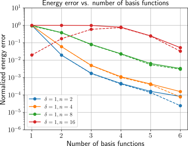
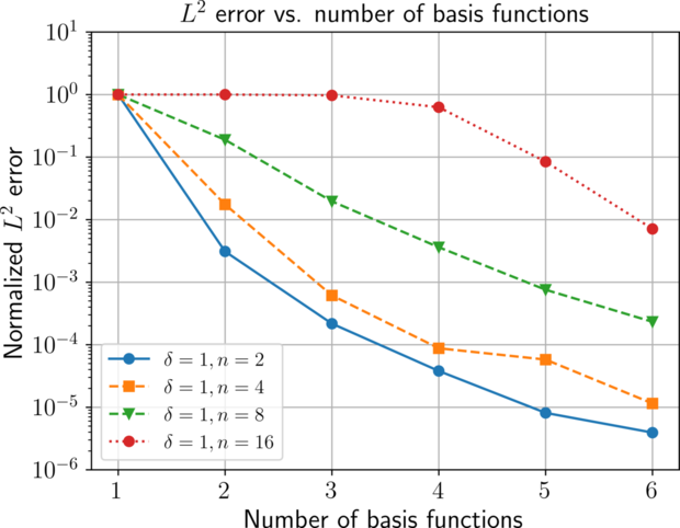
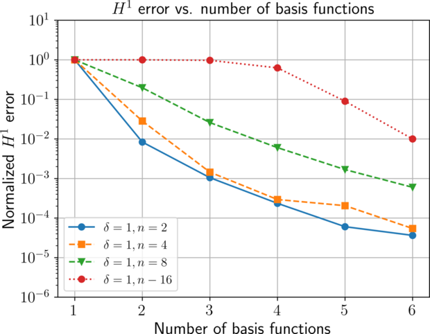
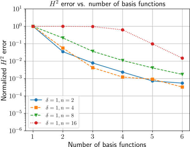
Figure 1: Errors with respect to the number of basis functions for $\delta=1$, $\mathcal{W}=L^{2}(\partial\Omega)$, and the sequence of problems $m=2,4,8,16$.

Example 2.3.

Consider a Poisson equation with exact solution given by the harmonic function $u_{m}(r,\theta)=r^{m}\sin(m\theta)$ in the unit circle. For a fixed $m\in\mathbb{N}$, a straightforward computation reveals that

$$||u_{m}||_{H^{2}(\Omega)}\propto m^{3/2},\;\;\;||u_{m}||_{H^{s}(\partial\Omega)}\propto m^{s},$$

and thus we have the ratio

(19) $$\delta||u_{m}||_{H^{s}(\partial\Omega)}/||u_{m}||_{H^{2}(\Omega)}\propto\delta m^{s-3/2}.$$

The case $\mathcal{W}=L^{2}(\partial\Omega)$ of the boundary penalization in (12) corresponds to $s=0$, and $m^{-3/2}\to 0$ as $m\to\infty$ which implies that the constant $C_{2}$ in Theorem 2.1 becomes vanishingly small. Indeed, the estimate (12) for the Poisson equation reads [11]

$$||u||_{H^{2}(\Omega)}\leqslant C(||f||_{L^{2}(\Omega)}+||g||_{H^{3/2}(\partial\Omega)}),$$

which indicates that the $H^{2}(\Omega)$ formulation of the Poisson equation based on (13) requires the choices $\mathcal{W}=H^{3/2}(\partial\Omega)$, $\mathcal{V}=L^{2}(\Omega)$, and $\mathcal{X}=H^{2}(\Omega)$.

One practical problem with choosing $\mathcal{W}$ to be of fractional order is the difficulty of evaluating the $H^{3/2}$-norm. For the present example where the true solution has the form $r^{m}\sin(m\theta)$, we take advantage of (19) and replace the $H^{3/2}$-norm by a weighted $L^{2}$-norm, i.e. $||u_{m}||_{H^{3/2}(\partial\Omega)}=m^{3/2}||u_{m}||_{L^{2}(\partial\Omega)}$. This is equivalent to taking $\mathcal{W}=L^{2}(\partial\Omega)$ and penalty parameter $\delta=(m^{3/2})^{2}=m^{3}$. Of course, this approach will not be possible in general but will suffice for the current example.

We first fix $\delta=1$, which corresponds to the case of $L^{2}$-penalization of the boundary conditions, and consider the sequence of PDEs corresponding to $m=2,4,8,16$ in order to demonstrate the gradual loss of coercivity for this problem. Figure 1 shows the error in various metrics for the Galerkin neural network method with formulation (13). For $m=2,4$ the $L^{2}$ boundary penalization is sufficient since $||u_{m}||_{L^{2}(\partial\Omega)},||u_{m}||_{H^{3/2}(\partial\Omega)}=\mathcal{O}(1)$. However, for larger $m$ we begin to observe reduced coercivity and the rate of convergence of the errors in all metrics.

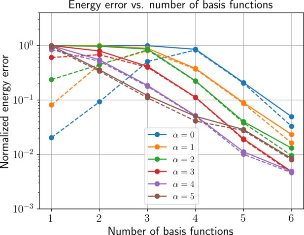
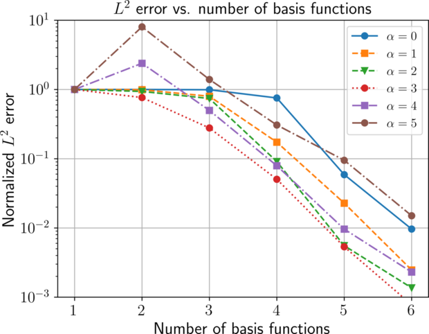
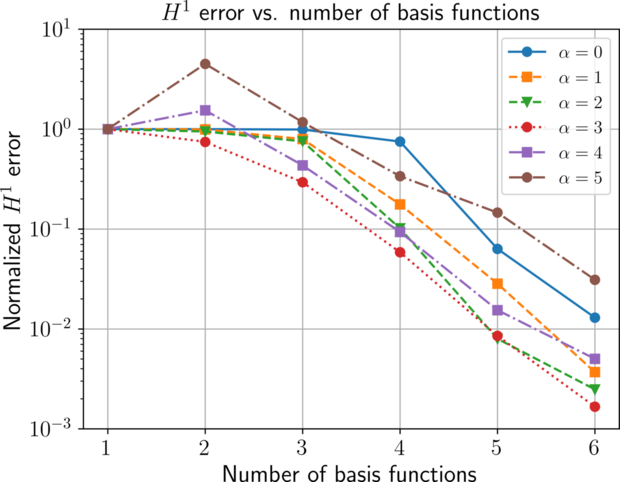
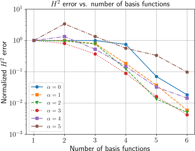
Figure 2: Errors with respect to the number of basis functions for several choices of penalty parameter $\delta=m^{\alpha}$.

Next, we fix $m=16$ and consider the choice $\delta=m^{\alpha}$ for $\alpha=0,1,2,3,4,5$ in order to demonstrate the effect of boundary penalization in different norms. Figure 2 shows the analogous results for this set of experiments. We observe that the error in the energy norm $|||\cdot|||:=a_{LS}(\cdot,\cdot)^{1/2}$ decreases monotonically regardless of the choice of $\alpha$ due to the guarantee of $u_{i}$ being the best approximation to $u$ from $S_{i}$. For $\alpha=0,1$ ($L^{2}(\partial\Omega)$ and approximate $H^{1/2}(\partial\Omega)$ boundary penalization, respectively), the errors in every metric are slow to converge. It is in this regime that the loss of coercivity is strongest. Rates improve for $\alpha=2$ (approximate $H^{1}(\partial\Omega)$ boundary penalization) and are optimal for $\alpha=3$ (approximate $H^{3/2}(\partial\Omega)$ boundary penalization). On the other hand, the overpenalization corresponding to $\alpha=4,5$ (approximate $H^{2}(\partial\Omega)$ and $H^{5/2}(\partial\Omega)$ boundary penalization, respectively) results in a loss of convergence and in particular, the clear loss of norm equivalence between $|||\cdot|||$ and $||\cdot||_{H^{k}(\Omega)},k\in\mathbb{N}$.

The above example illustrates the importance of using the correct norms that arise in the well-posedness of the problem. In practice, the presence of fractional norms presents difficulties but is possible using techniques such as those in [19]. However, generally speaking their computation is impractical and we instead utilize the highest possible integer Sobolev norm whose order is close to the order of the desired Sobolev norm. For instance, the $H^{1}(\partial\Omega)$ penalization in Figure 2 still performs quite well when compared to the optimal $H^{3/2}(\partial\Omega)$ penalization.

2.3 Extended neural network architectures

In what follows, we assume that the solution $u\in\mathcal{X}$ admits a representation of the form

(20) $$u(x)=u_{\infty}(x)+u_{\Psi}(x;\lambda),\;\;\;\;\;u_{\Psi}(x;\lambda):=\sum_{i=1}^{m}c_{\lambda,i}\Psi(x;\lambda_{i}),$$

where $u_{\infty}$ is the portion of the solution with high regularity and $u_{\Psi}$ the portion with low regularity of the form $\sum_{i}c_{\Psi,i}\Psi(\cdot;\lambda_{i})$. The solutions of many classical PDEs exhibit well-known structures $\Psi(x;\lambda_{i})$, where $\lambda$ is a parameter that depends on the specific form of the domain, boundary conditions, and coefficients of the PDE. For instance, for the Poisson equation, the singular part of the solution near corners of a polygonal domain is a sum of terms of the form $\Psi(r,\theta;\lambda)\propto r^{\lambda_{i}}\sin(\lambda_{i}\theta)$, where $\lambda_{i}$ depends on the interior angle at the corner. If such knowledge-based functions are available, then it makes sense for them to be incorporated into the Galerkin neural network framework. We shall exhibit the benefits of doing so in Section 3. The extended Galerkin neural network approach we shall describe in this section gives the flexibility to incorporate this problem-specific knowledge into the basic Galerkin neural neural method.

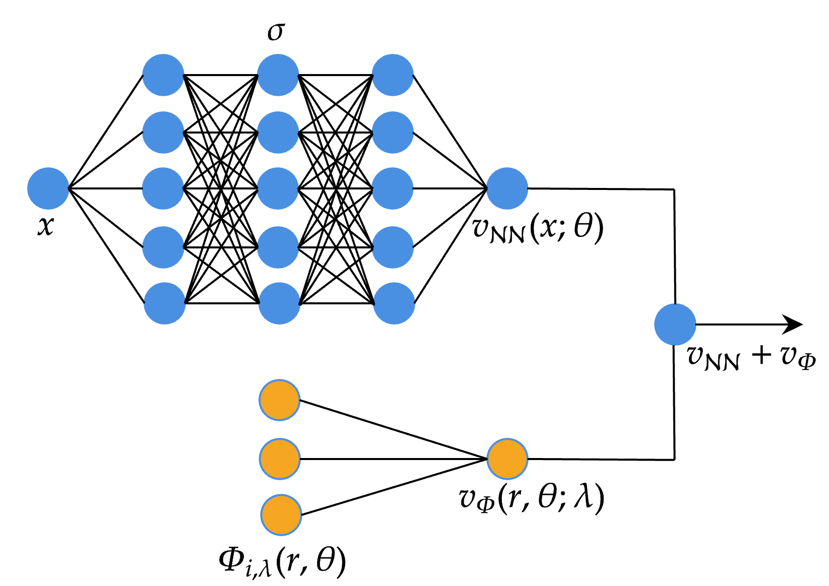
Figure 3: Extended neural network architecture for extended Galerkin neural networks.

For a given $\Phi\in\mathcal{X}$, let

(21) $$V_{m}^{\Phi}:=\{v\;:\;v(x)=\sum_{i=1}^{m}c_{\lambda,i}\Phi(x;\lambda_{i}),\;\mathbf{c}_{\lambda}\in\mathbb{R}^{m}\},$$

and, as in the basic Galerkin neural network in Section 2.1, we define the set of realizations whose parameters are bounded:

(22) $$V_{m}^{\Phi,C}:=\{v\in\tilde{V}_{m}^{\Phi}\;:\;||(\lambda,\mathbf{c}_{\lambda})||_{\Lambda}:=||\mathbf{c}_{\lambda}||_{\infty}+||\lambda||_{\infty}\leqslant C\}.$$

We then apply the Galerkin neural network framework in Section 2.1 using the augmented space $V_{\mathbf{n},L}^{\sigma,C}\oplus V_{n_{\lambda}}^{\Phi,C}$ and seek

(23) $$\varphi_{i}^{NN}=\operatorname*{arg\,max}_{v\in V_{\mathbf{n},L}^{\sigma,C_{1}}\bigoplus V_{n_{\lambda}}^{\Phi,C_{2}}\cap B}\langle r(u_{i-1}),v\rangle.$$

In order to ensure the existence of $\varphi_{i}^{NN}$, we require that the choice of $\Phi$ results in a continuous mapping from the parameter space $(\lambda,\mathbf{c}_{\lambda})$ into the set $V_{m}^{\Phi,C}$.

Lemma 2.4.

Let

$$\Lambda:=\left\{\lambda\in\mathbb{R}^{n_{\lambda}},\;\mathbf{c}_{\lambda}\in\mathbb{R}^{n_{\lambda}}\;:\;||(\lambda,\mathbf{c}_{\lambda})||_{\Lambda}:=||\mathbf{c}_{\lambda}||_{\infty}+||\lambda||_{\infty}\leqslant C\right\}.$$

Suppose the mapping $\mathcal{N}:(\Lambda,||\cdot||_{\Lambda})\to(V_{n_{\lambda}}^{\Phi,C},|||\cdot|||)$ defined by

$$\mathcal{N}(\lambda,\mathbf{c}_{\lambda})=\sum_{i=1}^{n_{\lambda}}c_{\lambda,i}\Phi(\cdot;\lambda_{i})$$

is continuous. Then $V_{n_{\lambda}}^{\Phi,C}$ is compact in $(\mathcal{X},|||\cdot|||)$.

The resulting function $\varphi_{i}^{NN}$ is then the sum of a neural network function $\varphi_{\sigma,i}^{NN}\in V_{\mathbf{n},L}^{\sigma,C}$ and a function $\varphi_{\Phi,i}^{NN}\in V_{n_{\lambda}}^{\Phi,C}$ belonging to the “knowledge-based” space. If the parameters $\lambda$ are unknown in advance, then one possibility is to learn them during the training step in a similar manner to $\mathbf{W}$ and $\mathbf{b}$:

(24) $$\lambda\leftarrow\lambda+\nabla_{\lambda}\left[\frac{\langle r(u_{i-1}),v(\cdot;\lambda)\rangle}{|||v(\cdot;\lambda^{)}|||}\right].$$

The corresponding coefficients $\mathbf{c}$ and $\mathbf{c}_{\lambda}$ are updated simultaneously by solving the following least squares system

(25) $$[\mathbf{c};\mathbf{c}_{\lambda}]=\operatorname*{arg\,min}_{\mathbf{c}\in\mathbb{R}^{n},\mathbf{c}_{\lambda}\in\mathbb{R}^{n_{\lambda}}}||\mathbf{A}[\mathbf{c};\mathbf{c}_{\lambda}]-\mathbf{F}||_{\ell^{2}}$$

for an appropriate matrix $\mathbf{A}$ and vector $\mathbf{F}$, and the approximation $u_{i}$ is obtained from the space of extended basis functions $S_{i}^{\Phi}:=\{u_{0}/|||u_{0}|||,\varphi_{\sigma,1}^{NN},\varphi_{\Phi,1}^{NN},\dots,\varphi_{\sigma,i}^{NN},\varphi_{\Phi,i}^{NN}\}$:

(26) $$u_{i}\in S_{i}^{\Phi}\;:\;a(u,v)=F(v)\;\;\;\forall v\in S_{i}^{\Phi}.$$

The solution may be written as a sum of smooth and singular parts $u_{i}=u_{\sigma,i}+u_{\Phi,i}$, where

(27) $$u_{\sigma,i}:=c_{\sigma,0}\frac{u_{0}}{|||u_{0}|||}+\sum_{j=1}^{i}c_{\sigma,j}\varphi_{\sigma,j}^{NN},\;\;\;u_{\Phi,i}:=\sum_{j=1}^{i}c_{\Phi,j}\varphi_{\Phi,j}^{NN}.$$

The effectiveness of the extended Galerkin neural network approach depends on the universal approximation properties of the neural networks as in the case of the basic Galerkin neural network approach. The following result, proved in [1] for the basic Galerkin neural network, is directly applicable to problems whose solutions take the form (20). The width $n$ appearing in Proposition 2.5 will depend on both the smooth and singular parts of the solution.

Proposition 2.5.

Let $0<\varepsilon<1$ be given. Then there exist $n(\varepsilon,u_{\infty}+u_{\Phi}-u_{i-1})\in\mathbb{N}$ and $C(\varepsilon,u_{\infty}+u_{\Psi}-u_{i-1})>0$ such that if $n\geqslant n(\varepsilon,u_{\infty}+u_{\Psi}-u_{i-1})$ and $C\geqslant C(\varepsilon,u_{\infty}+u_{\Psi}-u_{i-1})$, then $\varphi_{i}^{NN}$ given by (3) satisfies $|||\varphi_{i}-\varphi_{i}^{NN}|||\leqslant 2\varepsilon/(1-\varepsilon)$.

By way of contrast with the extended Galerkin neural network approach, the width $n$ depends only on the high regularity part of the solution. Thus, we expect the width of the network required to approximate $\varphi_{i}^{NN}$ to a given tolerance to be smaller than that required in Proposition 2.5 (see e.g. Section 3.1, Example 3.3).

The basis function $\varphi_{i}^{NN}$ satisfies the following approximation property.

Proposition 2.6.

Suppose that the following property holds: For each $\varepsilon>0$, there exists $n_{\lambda}(\varepsilon,\sum_{j=1}^{m}c_{\Psi,j}\Psi(\cdot;\lambda_{i}))\in\mathbb{N}$ and $C(\varepsilon,\sum_{j=1}^{m}c_{\Psi,j}\Psi(\cdot;\lambda_{i}))>0$ and $\tilde{\varphi}_{\Phi}\in\tilde{V}_{n_{\lambda}}^{\Phi}$ such that

(28) $$|||\sum_{j=1}^{m}c_{\Psi,j}\Psi(\cdot;\lambda_{i})-\tilde{\varphi}_{\Phi}|||\leqslant\varepsilon.$$

Then given $u_{0}\in(\mathcal{X},|||\cdot|||)$ and $L_{i}\in\mathbb{N}$, for each $\varepsilon>0$ there exists $\mathbf{n}^{(i)}(\varepsilon,u_{\infty}-u_{\sigma,i-1})\in\mathbb{N}^{L_{i}}$, $C_{1}(\varepsilon,u_{\infty}-u_{\sigma,i-1})$ as well as $n_{\lambda}^{(i)}(\varepsilon,u_{\Psi}-u_{\Phi,i-1})\in\mathbb{N}$, $C_{2}(\varepsilon,u_{\Psi}-u_{\Phi,i-1})>0$, and $\varphi_{i}^{NN}:=\varphi_{\sigma,i}^{NN}+\varphi_{\Phi,i}^{NN}\in V_{\mathbf{n}^{(i)},L_{i}}^{\sigma,C_{1}}\oplus V_{n_{\lambda}^{(i)}}^{\Phi,C_{2}}$ defined by (23) such that

(29) $$|||\varphi_{i}-\varphi_{i}^{NN}|||\leqslant\varepsilon.$$

Proof 2.7.

We partition the error by $\varphi_{i}=\varphi_{\sigma,i}+\varphi_{\Phi,i}$, where $\varphi_{\sigma,i}:=(u_{\infty}-u_{\sigma,i-1})/|||u-u_{i-1}|||$ and $\varphi_{\Phi,i}:=(u_{\Psi}-u_{\Phi,i-1})/|||u-u_{i-1}|||$ and first demonstrate that there exists a function $\hat{\varphi}\in V_{\mathbf{n}^{(i)},L_{i}}^{\sigma}\oplus V_{n_{\lambda,i}}^{\Phi}\cap B$ such that $|||\varphi_{i}-\hat{\varphi}|||\leqslant\varepsilon$. Applying the universal approximation theorem for multilayer feedforward networks [10] yields the existence of $\mathbf{n}(\varepsilon,u_{\infty}-u_{\sigma,i-1})\in\mathbb{N}^{L_{i}}$ and $\tilde{\varphi}_{\sigma}\in V_{\mathbf{n}^{(i)},L_{i}}^{\sigma}$ such that $|||\varphi_{\sigma,i}-\tilde{\varphi}_{\sigma}|||<\varepsilon/4$. To approximate $\varphi_{\Phi,i}$, we need only approximate $u_{\Psi}$ and $u_{\Phi,i-1}$. By (28), we can find $\tilde{n}_{\lambda}(\varepsilon,u_{\Psi})\in\mathbb{N}$ and $\tilde{\varphi}_{\Psi}\in\tilde{V}_{\tilde{n}_{\lambda}}^{\Phi}$ such that $|||u_{\Psi}-\tilde{\varphi}_{\Psi}|||<\varepsilon/4$, and since $u_{\Phi,i-1}\in\oplus_{j=1}^{i-1}V_{n_{\lambda}^{(j)}}^{\Phi}$ there exists $\eta\in V_{\sum_{j=1}^{i-1}n_{\lambda}^{(j)}}^{\Phi}$ such that $|||u_{\Phi,i-1}-\eta|||=0$. Setting $\tilde{\varphi}_{\Phi}:=\tilde{\varphi}_{\Psi}+\eta$, we have $|||\varphi_{\Phi,i}-\tilde{\varphi}_{\Phi}|||<\varepsilon/4$. Additionally, setting $\tilde{\varphi}:=\tilde{\varphi}_{\sigma}+\tilde{\varphi}_{\Phi}$, we have $|||\varphi_{i}-\tilde{\varphi}|||\leqslant\varepsilon/2$ and, by the reverse triangle inequality, $|||\tilde{\varphi}|||-1\in(-\varepsilon/2,\varepsilon/2)$.

We next demonstrate that the normalization of $\tilde{\varphi}=\tilde{\varphi}_{\sigma}+\tilde{\varphi}_{\Phi}$, which we shall define by

$$\hat{\varphi}:=\frac{\tilde{\varphi}_{\sigma}+\tilde{\varphi}_{\Phi}}{|||\tilde{\varphi}_{\sigma}+\tilde{\varphi}_{\Phi}|||},$$

is also an adequate approximation to $\varphi_{i}$. By the triangle inequality, we have

$$|||\varphi_{i}-\hat{\varphi}||| \leqslant|||\varphi_{\sigma,i}-\tilde{\varphi}_{\sigma}|||+|||\varphi_{\Phi,i}-\tilde{\varphi}_{\Phi}|||+|||\tilde{\varphi}-\frac{\tilde{\varphi}}{|||\tilde{\varphi}|||}|||$$

$$\leqslant\varepsilon/2+\frac{1}{|||\tilde{\varphi}|||}|||(|||\tilde{\varphi}|||-1)\tilde{\varphi}|||\leqslant\varepsilon.$$

Choose $C_{1}:=||\hat{\theta}||_{\mathcal{NN}}$ and $C_{2}:=||(\hat{\lambda},\mathbf{c}_{\hat{\lambda}})||_{\Lambda}$ where $\hat{\theta}$ and $(\hat{\lambda},\mathbf{c}_{\hat{\lambda}})$ are the parameters corresponding to the realizations $\tilde{\varphi}_{\sigma}/|||\tilde{\varphi}_{\sigma}+\tilde{\varphi}_{\Phi}|||$ and $\tilde{\varphi}_{\Phi}/|||\tilde{\varphi}_{\sigma}+\tilde{\varphi}_{\Phi}|||$, respectively. Additionally, choose $\mathbf{n}^{(i)}$ so that $\mathbf{n}^{(i)}_{j}\geqslant\mathbf{n}_{j}$ for $1\leqslant j\leqslant L_{i}$ and choose $n_{\lambda}^{(i)}\geqslant m+\sum_{j=1}^{i-1}n_{\lambda}^{(j)}$.

It remains to show that $\hat{\varphi}$ is sufficiently close in norm to the maximizer $\varphi_{i}^{NN}$. The argument does not differ from the corresponding proof for the basic Galerkin neural network framework in [1]. For completeness, we summarize the argument here. Since $\varphi_{i}^{NN}$ is the maximizer of $\langle r(u_{i-1}),\cdot\rangle=a(u-u_{i-1},\cdot)$, we have $a(\varphi_{i},\varphi_{i}^{NN})\geqslant a(\varphi_{i},v)$ for all $v\in V_{\mathbf{n}^{(i)},L_{i}}^{\sigma,C_{1}}\oplus V_{n_{\lambda}^{(i)}}^{\Phi,C_{2}}\cap B$ and

$$|||\varphi_{i}-\varphi_{i}^{NN}|||^{2} =|||\varphi_{i}|||^{2}-a(\varphi_{i},\varphi_{i}^{NN})+|||\varphi_{i}^{NN}|||^{2}$$

$$\leqslant|||\varphi_{i}|||^{2}-a(\varphi_{i},\hat{\varphi})+|||\hat{\varphi}|||^{2}=|||\varphi_{i}-\hat{\varphi}|||^{2}\leqslant\varepsilon^{2}.$$

We obtain the following result demonstrating the convergence of the extended Galerkin neural network.

Corollary 2.8.

The approximation $u_{i}$ given in (26) satisfies the estimate

(30) $$|||u-u_{i}|||\leqslant|||u-u_{0}|||\cdot\min\left\{1,\varepsilon\right\}^{i}.$$

Moreover, if $\varepsilon<1$, then each $\varphi_{i}^{NN}$ satisfies

(31) $$\langle r(u_{i-1}),\varphi_{i}^{NN}\rangle\leqslant|||u-u_{i-1}|||\leqslant\frac{1}{1-\varepsilon}\langle r(u_{i-1}),\varphi_{i}^{NN}\rangle.$$

Proof 2.9.

The proof of (30) follows from [1, Proposition 2.6]. The upper bound of (31) follows from the fact that

$$\left|\langle r(u_{i-1}),\varphi_{i}^{NN}-|||u-u_{i-1}|||\right|\leqslant|||u-u_{i-1}|||\cdot|||\varphi_{i}^{NN}-\varphi_{i}|||=\varepsilon|||u-u_{i-1}|||$$

while the lower bound follows from the observation that $\langle r(u_{i-1}),\varphi_{i}^{NN}\rangle:=a(u-u_{i-1},\varphi_{i}^{NN})\leqslant|||u-u_{i-1}|||$.

3 Applications

We consider several indefinite and non-self adjoint boundary value problems and present well-posed least squares variational formulations for each of them. All hyperparameters for each example are provided in Appendix B. Of particular interest to us are problems whose solutions contain singular features, for instance due to low-regularity data or nonconvex domain corners.

As a motivating example, consider the incompressible stationary Stokes flow in velocity-pressure form given by the boundary value problem

(32) $$\begin{dcases}-\Delta\mathbf{u}+\nabla p=\mathbf{f}&\text{in}\;\Omega\\ \text{div}\;\mathbf{u}=g&\text{in}\;\Omega\\ \mathbf{u}=\mathbf{u}_{D}&\text{on}\;\partial\Omega,\end{dcases}$$

where $\Omega\subset\mathbb{R}^{2}$ is a bounded and connected polygonal domain, $\mathbf{u}$ is the fluid velocity, and $p$ the fluid pressure. To ensure solvability of (32), we require the compatibility condition $\int_{\Omega}g\;d\mathbf{x}=-\int_{\partial\Omega}\mathbf{u}_{D}\cdot\mathbf{n}\;ds$.

The most natural variational formulation associated with (32) is to seek $(\mathbf{u},p)\in\mathbf{H^{1}_{0}}(\Omega)\times(L^{2}(\Omega)/\mathbb{R})$ such that

(33) $$\begin{dcases}(\nabla\mathbf{u},\nabla\mathbf{v})_{\Omega}-(p,\text{div}\;\mathbf{v})_{\Omega}&=(\mathbf{f},\mathbf{v})_{\Omega}+(\mathbf{u}_{D},\mathbf{v})_{\partial\Omega}\\ (\text{div}\;\mathbf{u},q)_{\Omega}&=(g,q)_{\Omega}\end{dcases}$$

for all $(\mathbf{v},q)\in\mathbf{H^{1}_{0}}(\Omega)\times(L^{2}(\Omega)/\mathbb{R})$. Formulation (33) is not SPD and thus we must use (13) in conjunction with Galerkin neural networks. However, if $\Omega$ contains nonconvex corners, then $\mathbf{u}\notin\mathbf{H^{2}}(\Omega)$ and $p\notin H^{1}(\Omega)$, and the spaces $\mathcal{X}$, $\mathcal{V}$, and $\mathcal{W}$ must be chosen carefully to account for the reduced regularity.

3.1 Poisson equation

We demonstrate the construction of a well-posed weighted least squares variational formulation for the Poisson equation:

(34) $$\begin{dcases}-\Delta u=f&\text{in}\;\Omega\\ u=g&\text{on}\;\partial\Omega.\end{dcases}$$

We consider the case where $\Omega$ is a polygon with vertices $\{x^{(i)}\}_{i=1}^{M}$.

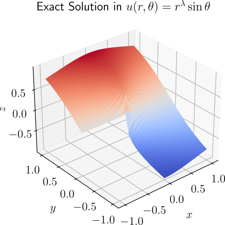
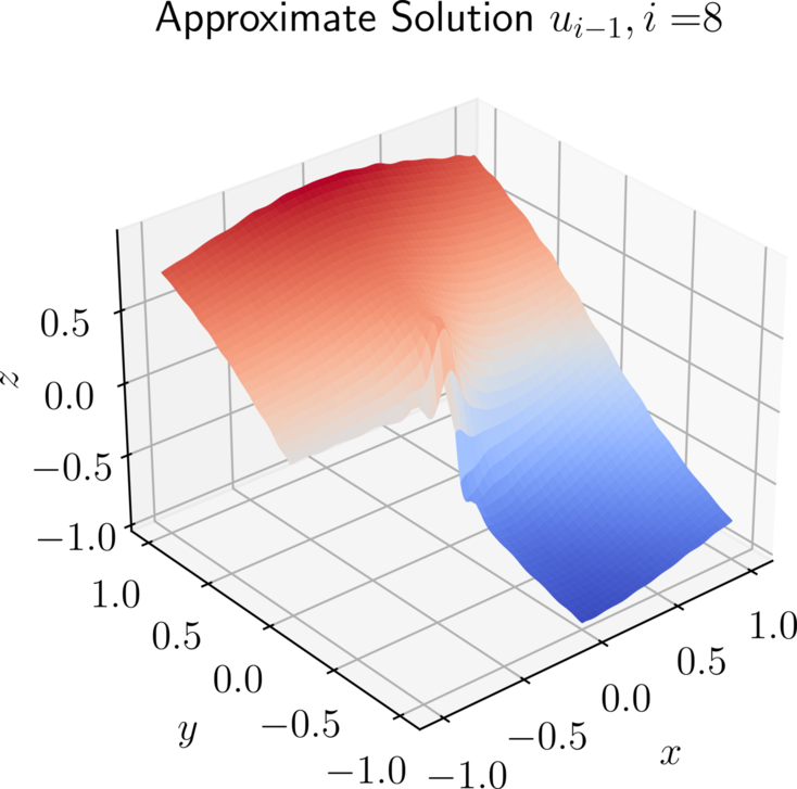
Figure 4: The true solution $u(r,\theta)=r^{\lambda}\sin{\theta}$ (left) and approximate solutions obtain using Galerkin neural networks and (36) with $\beta=0$ (middle) and $\beta=1$ (right).

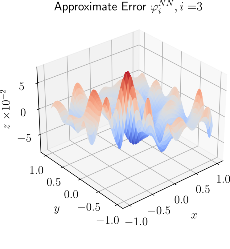
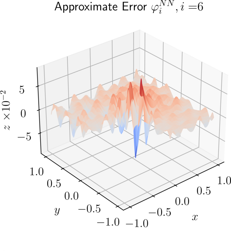
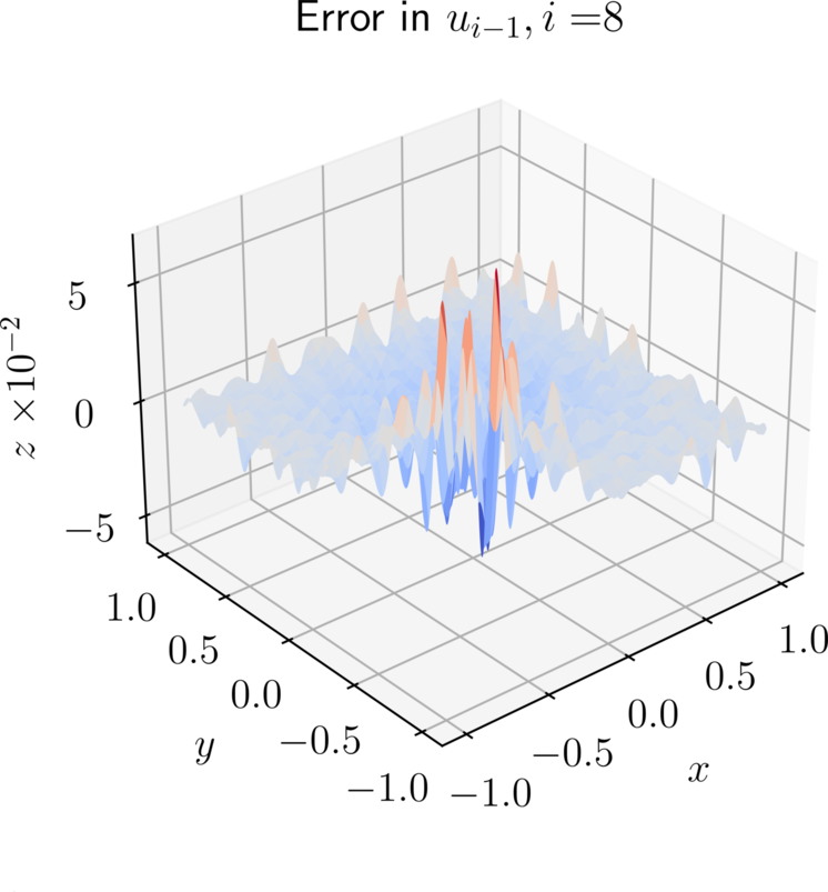
Figure 5: Example 3.2: for $\beta=0$, the errors $u-u_{i-1}$ and learned basis functions $\varphi_{i}^{NN}$.

3.1.1 Regularity and variational formulation

The following a priori estimate is a result of Kondrat’ev [11].

Theorem 3.1.

[11] Suppose $f\in L^{2}_{\beta}(\Omega)$ and $g\in H^{3/2}_{\beta}(\partial\Omega)$. Then (34) admits a unique solution $u\in H^{2}_{\beta}(\Omega)$ and

$$||u||_{H^{2}_{\beta}(\Omega)}\leqslant C(||f||_{L^{2}_{\beta}(\Omega)}+||g||_{H^{3/2}_{\beta}(\partial\Omega)}),$$

for some $C>0$ independent of $u$, $f$, and $g$, where

$$||u||_{H^{3/2}_{\beta}(\partial\Omega)}:=\inf_{U|_{\partial\Omega}=u}||U||_{H^{2}_{\beta}(\Omega)}.$$

The spaces $H^{s}_{\beta}(\Omega)$ are weighted Sobolev spaces defined by

(35) $$H^{s}_{\beta}(\Omega):=\left\{u\;:\;\prod_{i=1}^{M}r_{i}^{\beta-s+|\alpha|}D^{\alpha}u\in L^{2}(\Omega),\;0\leqslant|\alpha|\leqslant s\right\},$$

where $r_{i}$ is the local radial coordinate centered at vertex $x^{(i)}$. In what follows, we will commonly use $(\cdot,\cdot)_{\beta,\Omega}$ to denote the $L^{2}_{\beta}(\Omega)$ inner product. We propose the weighted least squares variational formulation given by

$$u\in H^{2}_{\beta}(\Omega)\;:\;(\Delta u,\Delta v)_{\beta,\Omega} +(u,v)_{H_{\beta}^{3/2}(\partial\Omega)}=-(f,\Delta v)_{\beta,\Omega}+(g,v)_{H_{\beta}^{3/2}(\partial\Omega)}$$

(36) $$\hskip 170.71652pt\forall v\in H^{2}_{\beta}(\Omega).$$

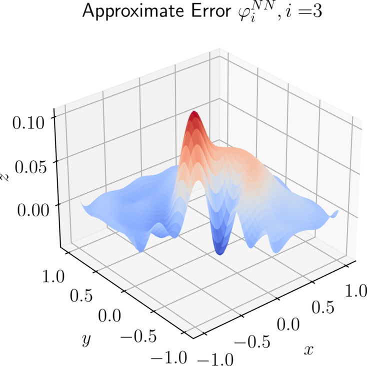
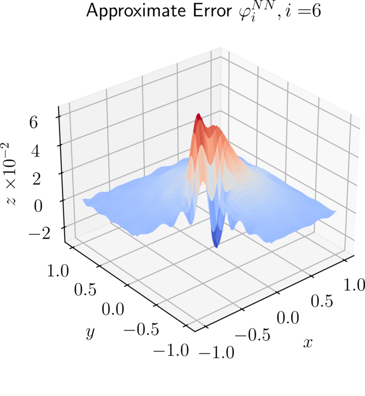
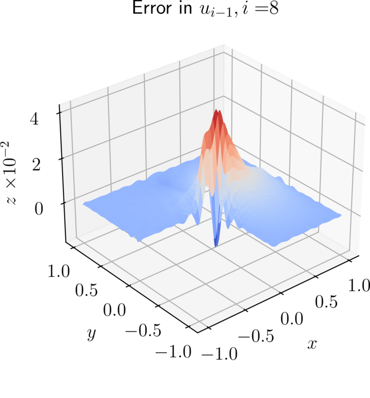
Figure 6: Example 3.2: for $\beta=1$, the errors $u-u_{i-1}$, learned basis functions $\varphi_{i}^{NN}$, and $L^{2}$- and energy norm errors.

Example 3.2.

We consider the case of the true solution $u(r,\theta)=r^{\lambda}\sin{\theta}$ for $\lambda=1/4$ in the domain $\Omega=(-1,1)^{2}\backslash(-1,0)^{2}$. In this case, $f\notin L^{2}(\Omega)$ but $f\in L^{2}_{\beta}(\Omega)$ for $\beta>1-\lambda$. We demonstrate that if $\beta=0$ in (36), then the approximation obtained is incorrect and does not converge to the true solution. Figure 4 shows the approximation using 8 basis functions.

We observe spurious oscillations of the approximation near $x=0$ when $\beta=0$ which are largely removed when $\beta=1$. Figures 5-6 show the true errors $u-u_{i-1}$ and basis functions $\varphi_{i}^{NN}$ for $\beta=0$ and $\beta=1$, respectively. We observe that in the $\beta=0$ case, the learned basis functions contain many high frequency modes not present in the corresponding error functions. In the $\beta=1$ case, the basis functions take on large values near $x=0$ and correctly identify the presence of error the approximation of the singularity, but convergence is still slow.

Figure 7: Example 3.3: for $\beta=4/3$, the approximate solutions $u_{i}$ and learned basis functions $\varphi_{i}^{NN}$.

3.1.2 Knowledge-based functions

Suppose $\Omega$ contains a single corner of interest $x^{(0)}$ with interior angle $\alpha^{(0)}$. For instance, the $L$-shaped domain $(-1,1)^{2}\backslash(-1,0)^{2}$ contains a nonconvex corner with angle $\alpha^{(0)}=3\pi/2$ at the origin. Solutions of (34) in such a domain have the well-known structure

(37) $$u(x,y)=\sum_{\lambda_{j}}c_{\lambda_{j}}r^{\lambda_{j}}\sin(\lambda_{j}\theta)+u^{*}(x,y),$$

where $u^{*}\in H^{2}(\Omega)$ and $\lambda_{n}$ are the eigenvalues of the operator pencil corresponding to the Laplacian operator [12]. The eigenvalues are given by

$$\lambda_{j}=\frac{j\pi}{\alpha^{(0)}},\;\;\;j=1,2,3,\dots.$$

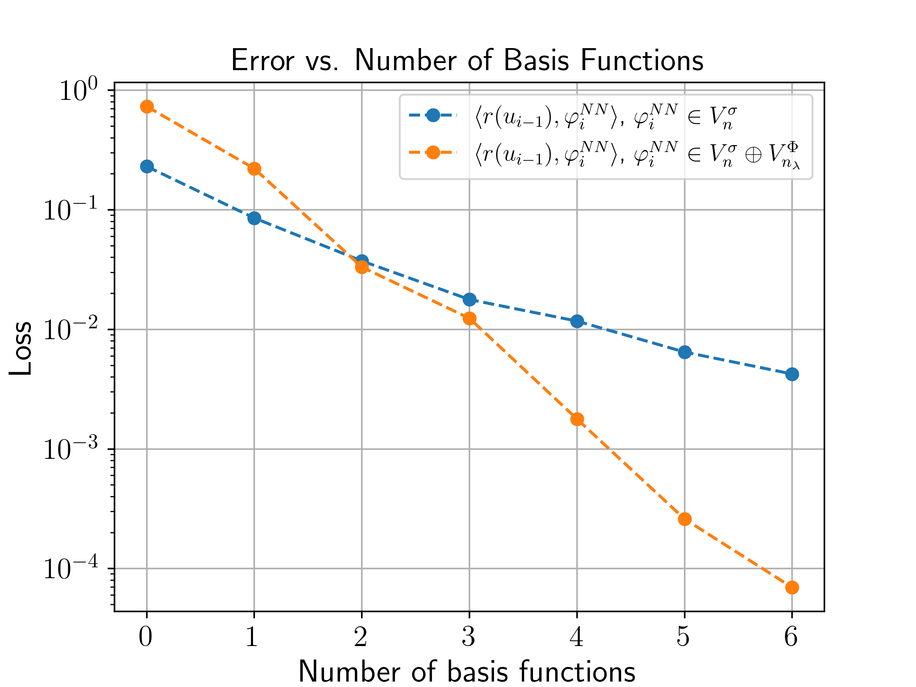
Figure 8: Example 3.3: for $\beta=4/3$ and singular neural network architecture, the approximate solutions $u_{i}$ and learned basis functions $\varphi_{i}^{NN}$.

Example 3.3.

We consider the problem with homogeneous Dirichlet boundary condition in the domain $\Omega=(-1,1)^{2}\backslash(-1,0)^{2}$ and data $f=1$. This problem was already considered in [1] for which the usual $H^{1}$ variational formulation of the Poisson equation was utilized. Nevertheless, this problem demonstrates many of the explemary singular features we wish to approximate and serves as an excellent example for how to utilize knowledge-based functions in the Galerkin-neural network framework.

While there is no closed form solution to this problem, we provide the value of the a posteriori error indicator $\langle r(u_{i-1}),\varphi_{i}^{NN}\rangle$ for each basis function learned as well as the basis functions $\varphi_{i}^{NN}$ themselves, which provide a function representation of the error $u-u_{i-1}$. Figure 7 shows the first several basis functions using a standard feedforward neural network for learning each basis function. We observe that the approximation converges quite slowly near $x=0$ and the basis functions $\varphi_{i}^{NN}$ show that the magnitude of the pointwise error is large in the vicinity of the singularity.

Next, we repeat the simulation, this time with an augmented neural network architecture. Namely, we compute $\varphi_{i}^{NN}$ according to (23) with $\Phi(r,\theta;\lambda)=r^{\lambda}\sin(\lambda\theta)$. Since the eigenvalues are known, we simply take $\lambda_{j}=2j/3$ and $n_{\lambda}=20$. However, we shall demonstrate in Section 4 how Galerkin neural networks may be used to approximate the values of $\lambda$ when they are unknown. Figure 8 shows the analogous results to Figure 7. We observe significantly faster convergence and the approximate pointwise errors decrease steadily from $\mathcal{O}(10^{-2})$ to $\mathcal{O}(10^{-5})$. Additionally, we note that the singularity is clearly captured correctly by the knowledge-based functions.

3.2 Stokes flow

The next application we consider is the incompressible steady Stokes flow (32).

3.2.1 Regularity and variational formulation

Schwab and Guo proved the following result in [9] for a polygonal domain $\Omega$.

Theorem 3.4.

[9] Suppose $\mathbf{f}\in\mathbf{L^{2}_{\beta}}(\Omega)$, $g\in H^{1}_{\beta}(\Omega)$, $\mathbf{u}_{D}\in\mathbf{H^{3/2}_{\beta}}(\partial\Omega)$, and $\int_{\Omega}g\;d\mathbf{x}=-\int_{\partial\Omega}\mathbf{u}_{D}\cdot\mathbf{n}\;ds$. Then (32) admits a unique solution $(\mathbf{u},p)\in\mathbf{H^{2}_{\beta}}(\Omega)\times H^{1}_{\beta}(\Omega)/\mathbb{R}$ and

(38) $$||\mathbf{u}||_{\mathbf{H^{2}_{\beta}}(\Omega)}+||p||_{H^{1}_{\beta}(\Omega)}\leqslant C(||\mathbf{f}||_{\mathbf{L^{2}_{\beta}}(\Omega)}+||g||_{H^{1}_{\beta}(\Omega)}+||\mathbf{u}_{D}||_{\mathbf{H^{3/2}_{\beta}}(\Omega)})$$

for some $C>0$ independent of $\mathbf{u}$, $p$, $\mathbf{f}$, $g$, and $\mathbf{u}_{D}$.

Most notable is that (3.4) suggests that the residual of the incompressibility equation in (32) should actually be taken in the $H^{1}_{\beta}$ norm, which leads to the continuous and coercive formulation: seek $(\mathbf{u},p)\in\mathbf{H^{2}_{\beta}}(\Omega)\times H^{1}_{\beta}(\Omega)/\mathbb{R}$ such that

$$(-\Delta\mathbf{u}+\nabla p,- \Delta\mathbf{v}+\nabla q)_{\beta,\Omega}+(\text{div}\;\mathbf{u},\text{div}\;\mathbf{v})_{H^{1}_{\beta}(\Omega)}+(\mathbf{u},\mathbf{v})_{H^{3/2}_{\beta}(\partial\Omega)}$$

$$=(\mathbf{f},-\Delta\mathbf{v}+\nabla q)_{\beta,\Omega}+(g,\text{div}\;\mathbf{v})_{H^{1}_{\beta}(\Omega)}+(\mathbf{u}_{D},\mathbf{v})_{\mathbf{H^{3/2}_{\beta}}(\Omega)}$$

for all $(\mathbf{v},q)\in\mathbf{H^{2}_{\beta}}(\Omega)\times H^{1}_{\beta}(\Omega)/\mathbb{R}$. For ease of notation, we set $X:=\mathbf{H^{2}_{\beta}}(\Omega)\times H^{1}_{\beta}(\Omega)/\mathbb{R}$ endowed with the norm $||(\mathbf{v},q)||_{X}:=(||\mathbf{v}||_{H^{2}_{\beta}(\Omega)}^{2}+||q||_{H^{1}_{\beta}(\Omega)}^{2})^{1/2}$ and define the bilinear operator $B:X\times X\to\mathbb{R}$ by

(39) $$B((\mathbf{u},p),(\mathbf{v},q)):=(-\Delta\mathbf{u} +\nabla p,-\Delta\mathbf{v}+\nabla q)_{\beta,\Omega}$$

$$+(\text{div}\;\mathbf{u},\text{div}\;\mathbf{v})_{H^{1}_{\beta}(\Omega)}+(\mathbf{u},\mathbf{v})_{H^{3/2}_{\beta}(\partial\Omega)}$$

and the linear operator $L:X\to\mathbb{R}$ by

(40) $$L((\mathbf{v},q)):=(\mathbf{f},-\Delta\mathbf{v}+\nabla q)_{\beta,\Omega}+(g,\text{div}\;\mathbf{v})_{H^{1}_{\beta}(\Omega)}+(\mathbf{u}_{D},\mathbf{v})_{\mathbf{H^{3/2}_{\beta}}(\Omega)}.$$

3.2.2 Knowledge-based functions

Many features of interest in the Stokes flow develop in the corners of $\Omega$, including singularities at reentrant corners and eddies in convex corners that are driven by the far-field flow. In these cases, the solution structure is well-known. Noting that the velocity is the curl of the streamfunction $\psi$, $\mathbf{u}=\nabla^{\perp}\psi$, and that the streamfunction satisfies a biharmonic equation, the streamfunction takes the form

(41) $$\psi(x,y)=\sum_{j=1}^{M}\chi(r^{(j)})\sum_{\lambda_{n}^{(j)}}c_{\lambda_{n}^{(j)}}r^{\lambda_{n}^{(j)}}\Psi_{\lambda_{n}^{(j)}}(\theta^{(j)})+\psi^{*}(x,y),$$

where $(r^{(j)},\theta^{(j)})$ are the local polar coordinates centered at $x^{(j)}$, $\{\lambda_{n}^{(j)}\}$ are the eigenvalues associated with the operator pencil of the biharmonic operator at vertex $x^{(j)}$ and $\Psi_{\lambda_{n}^{(j)}}$ are the corresponding generalized eigenfunctions, $\chi_{j}\in C^{s}(\bar{\Omega})$ is a cutoff function centered at $x^{(j)}$, and $\psi^{*}\in H^{4}(\Omega)$. The corresponding velocity and pressure solutions are derived from (41). See Appendix A for full details.

For $\lambda\neq 0,1,2$, the eigenvalues of the biharmonic operator pencil at $x^{(j)}$ are given implicitly by [6]

(42) $$\sin^{2}((\lambda-1)\alpha_{j})-(\lambda-1)^{2}\sin^{2}(\alpha_{j})=0,$$

where $\alpha_{j}$ is the interior angle of $x^{(j)}$. The eigenfunctions [6] are given by

(43) $$\Psi_{\lambda}(\theta)=A\sin(\lambda\theta)+B\cos(\lambda\theta)+C\sin((\lambda-2)\theta)+D\cos((\lambda-2)\theta),$$

with the constants $A,B,C,D$ chosen so that $\Phi$ satisfies suitable boundary conditions.

Figure 9: Channel with triangular cavity for Example 3.5. The rectangle channel is described by $(-2,2)\times(0,2)$ while the triangular cavity has vertices at $(-1,0)$, $(1,0)$, and $(-3,0)$.

In the case when $\alpha_{j}\lessapprox 146^{\circ}$, solutions of (42) are complex and we replace $r^{\lambda_{n}}\Psi_{\lambda_{n}}(\theta)$ by $\mathfrak{Re}[r^{\lambda_{n}}\Psi_{\lambda_{n}}(\theta)]$ in (41). Interestingly, complex eigenvalues are associated with infinite sequences of eddies in the flow due to disturbances in the far field. This behavior is described mathematically by, for instance

$$\mathfrak{Re}(r^{a+ib}\cos((a+ib)\theta))=r^{a}\cos(b\log{r})\cos(a\theta)\cosh(b\theta).$$

One can show, as in [16], that each successive eddy decays exponentially in magnitude. Thus, Stokes flows in polygonal domains must be resolved to a very high degree of accuracy in order to adequately capture these eddies.

Example 3.5.

Let $\Omega$ be the channel with triangular cavity as shown in Figure 9. The flow takes a parabolic profile prescribed at the inflow and outflow. Namely, the boundary conditions are

$$u_{1}(x,y)=\begin{dcases}y(2-y),&x=-2\;\text{or}\;2\\ 0,&\text{else},\end{dcases}\;\;\;\;\;\;u_{2}(x,y)=0.$$

We specify $\mathbf{f}=\mathbf{0}$ and $g=0$, in which case $2\text{div}\;\epsilon(\mathbf{u})=\Delta\mathbf{u}$. At the reentrant corners, we expect a singularity to manifest in both the velocity and pressure. At the bottom corner, we expect infinitely cascading eddies driven by the channel flow. As described in Section 3.2.2, we shall supplement the standard feedforward network with $\Psi(r,\theta;\lambda)=\chi(r)\mathfrak{Re}[r^{\lambda}\Psi_{\lambda}(\theta)]$ in the bottom corner and $\Psi(r,\theta;\lambda)=\chi(r)r^{\lambda}\Psi_{\lambda}(\theta)$ at the reentrant corners. The exact values of $\lambda$ are $\lambda=1.58223$ in the reentrant corners and $\lambda=7.56813+3.37941i$ in the bottom corner. Precise details may be found in Appendix A. As with Example 3.3, we shall demonstrate in Section 4 how these values of $\lambda$ may be approximated using Galerkin neural networks in the event that they are unknown.

Figure 10: Example 3.5: velocity and pressure with $\beta=0$ (top) and $\beta=5/3$ (bottom) in (39).

We first demonstrate the importance of choosing the Sobolev weight parameter $\beta$ appropriately. In contrast with Example 3.2, this example contains smooth data $f$ and $g$ and continuous data $\mathbf{u}_{D}$. Figure 10 shows the approximated velocities and pressures for $\beta=0$. We shall use $\varphi_{1,i}^{NN}$, $\varphi_{2,i}^{NN}$, and $q_{i}^{NN}$ to denote the $i$th basis functions for the velocities and pressure, respectively. The resulting velocity and pressure fields in Figure 10 show that even after learning six basis functions, the flow is nonphysical; we expect a near constant velocity $u_{1}$ along the $x$-direction in the channel. Figure 10 also shows the analogous results for $\beta=5/3$. Despite not adequately capturing the singularities and the expected sequence of eddies, the approximate solutions do not exhibit spurious oscillations and the behavior in the channel is as expected.

Figure 11: Example 3.5: velocity and pressure with $\beta=5/3$ in (39) and basis functions learned from extended neural network with knowledge-based functions.

We fix $\beta=5/3$ next and approximate the solution using six basis functions learned by extended Galerkin neural networks. We remarkably observe that with the supplemental activation functions, i.e. $\varphi_{1,i}^{NN},\varphi_{2,i}^{NN},q_{i}^{NN}\in V_{\mathbf{n},L}^{\sigma}\oplus V_{n_{\lambda}}^{\Phi}$, both the singular features at the reentrant corners and the eddies in the cavity are captured accurately. In fact, as Figure 11 shows, we are able to capture infinitely many eddies. The basis functions used to approximate the velocities and pressures are shown in Figure 12.

Finally, when $\beta$ is too large, the solution space contains functions which may have worse singular behavior than the true solution due to the strong damping effect of $r^{\beta}$ on the singularities. In particular, the bilinear operator $B$ may admit as arguments functions with far stronger singularities than those of the true solution. We show the results for $\beta=4$ in Figure 13.

Figure 12: Example 3.5: velocity and pressure basis functions with $\beta=5/3$ in (39) and basis functions learned from extended neural network with knowledge-based functions.

Figure 13: Example 3.5: velocity and pressure basis functions with $\beta=4$ in (39) and basis functions learned from extended neural network with knowledge-based functions.

4 Extended Galerkin neural networks with learning of knowledge-based functions

In the numerical examples in Section 3, we approximated the solutions from the set $V_{\mathbf{n},L}^{\sigma}\oplus V_{n_{\lambda}}^{\Phi}$, where $V_{n_{\lambda}}^{\Phi}$ denotes the span of knowledge-based functions $\Phi(x;\lambda)$:

$$V_{n_{\lambda}}^{\Phi}:=\{v\;:\;v(x)=\sum_{i=1}^{n_{\lambda}}c_{\lambda,i}\Phi(x;\lambda_{i}),\;\mathbf{c}_{\lambda}\in\mathbb{R}^{n_{\lambda}}\}.$$

We utilized exact known values of $\lambda$ when including these functions in the approximation space. However, in many applications some information about the structure of $\Phi$ may be known while the parameters $\lambda$ may be unknown or difficult to compute exactly. In this section, we demonstrate how extended Galerkin neural networks may be applied to the previously studied examples in order to approximate $\lambda$.

4.1 Poisson equation

We revisit Example 3.3 in which the knowledge-based functions took the form

$$\Phi(r,\theta;\lambda)=r^{\lambda}\sin(\lambda\theta).$$

The exact values of $\lambda$ are given by $2/3,4/3,\dots,2j/3,\dots$. We focus only the smallest value of $\lambda$ which describes the asymptotic behavior of $\Phi$ and note that the feedforward part of the neural network, $V_{\mathbf{n},L}^{\sigma}$, is capable of approximating the smoother behavior of $\Phi$ for larger values of $\lambda$.

Example 4.1.

We again consider the L-shaped domain $\Omega=(-1,1)^{2}\backslash(-1,0)^{2}$ with data $f=1$ and homogeneous Dirichlet boundary conditions. Each Galerkin neural network basis function is obtained according to (23) with $\lambda$ being a trainable parameter. The initial value of $\lambda$ is drawn from the uniform distribution $\mathcal{U}(0,1)$. Figure 14 shows how $\lambda_{1}$ changes value during the backpropagation step of training over 20 independent runs. In each case $\lambda_{1}$ moves toward the true value of $2/3$.

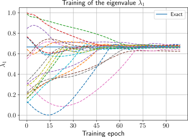
Figure 14: Example 4.1: training of $\lambda_{1}$ and over several runs with initialization $\lambda\sim\mathcal{U}(0,1)$.

4.2 Stokes flow around a nonconvex corner

Example 4.2.

Analogous to Example 4.1, we demonstrate how to learn the knowledge-based functions for the Stokes flow around a nonconvex corner. We consider the circular sector domain $\Omega=\{(r,\theta)\;:\;0<r<1,\;0<\theta<\pi+\alpha^{(0)}\}$, $\alpha^{(0)}=\arccos(1/\sqrt{10})$ with $\mathbf{f}=\mathbf{0}$ and $g=0$. The boundary condition for the velocity is given by

$$\mathbf{u}(\theta)=\begin{bmatrix}-\frac{1}{2\alpha^{(0)}}\theta^{2}+\theta\\ \frac{-2\alpha^{(0)}-1}{4(\alpha^{(0)})^{2}}\theta^{3}+\theta^{2}+\theta\end{bmatrix}.$$

This example may be viewed as a localized BVP with artificial boundary conditions.

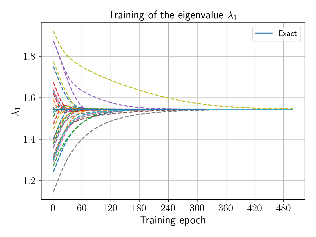
Figure 15: Eigenvalue training progress for Example 4.2 with initialization $\lambda\sim\mathcal{U}(\lambda_{\text{exact}}-1/3,\lambda_{\text{exact}}+1/3)$.

We approximate the solution to this example using a feedforward network augmented with the knowledge-based function $\Phi(r,\theta;\lambda)=r^{\lambda}\Psi_{\lambda}(\theta)$, where $\Psi_{\lambda}$ is given in Appendix A for the velocity and pressure. We initialize $\lambda$ away from its true value as in Example 4.1 in order to demonstrate that the true eigenvalue of the singular part of the Stokes operator may also be learned by the neural network. Importantly, the singular-behavior of the solution at the origin should be localized with a cutoff function, namely in (21) we take

$$\tilde{V}_{m}^{\Phi}:=\left\{v\;:\;v(x)=\sum_{i=1}^{m}c_{\lambda,i}\chi(r)\Phi(x;\lambda_{i}),\;\mathbf{c}_{\lambda}\in\mathbb{R}^{m}\right\},$$

where $\chi$ is a $C^{2}$ cutoff function satisfying $\chi(r)=1$ for $r<r_{0}$, $\chi(r)=0$ for $r>r_{1}$.

Figure 15 shows the training progress of $\lambda$ over 30 trials with $\lambda$ initialized according to the uniform distribution $\mathcal{U}(\lambda_{\text{exact}}-1/3,\lambda_{\text{exact}}+1/3)$. We observe that in each trial, $\lambda$ converges to the true value.

4.3 Stokes flow in a convex corner induced by disturbance at a large distance

Example 4.3.

We now demonstrate how to learn the knowledge-based functions for the Stokes flow in a convex corner induced by flow at a large distance. The localized domain $\Omega$ is the triangular wedge with vertices $(1,0)$, $(-1,0)$, and $(-3,0)$. The boundary condition for the velocity is a homogeneous Dirichlet condition along the diagonal edges of the wedge and $\mathbf{u}(x,y)=[(1-x)(1+x),0]^{T}$ along the top edge. We again specify $\mathbf{f}=\mathbf{0}$ and $g=0$.

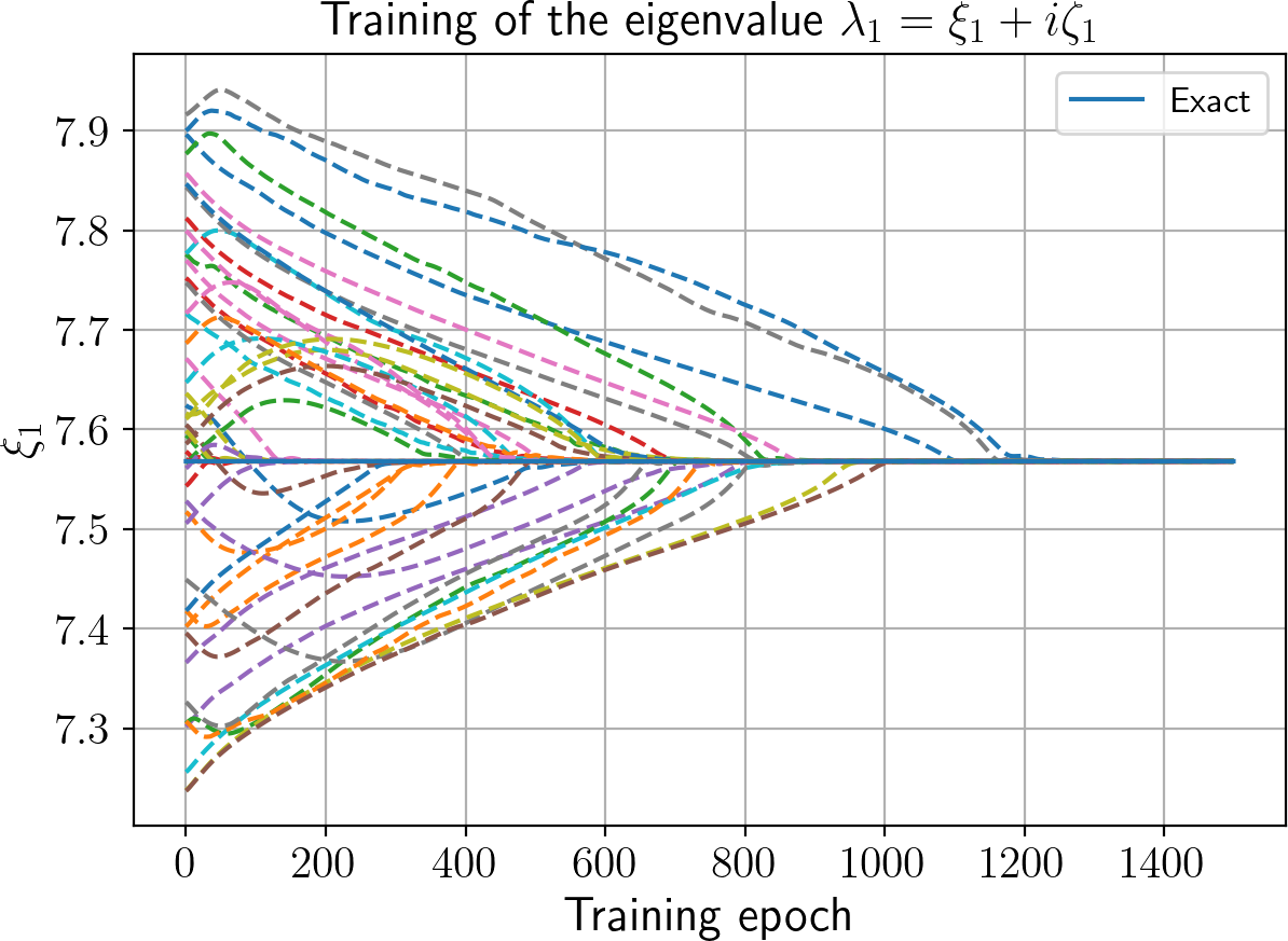
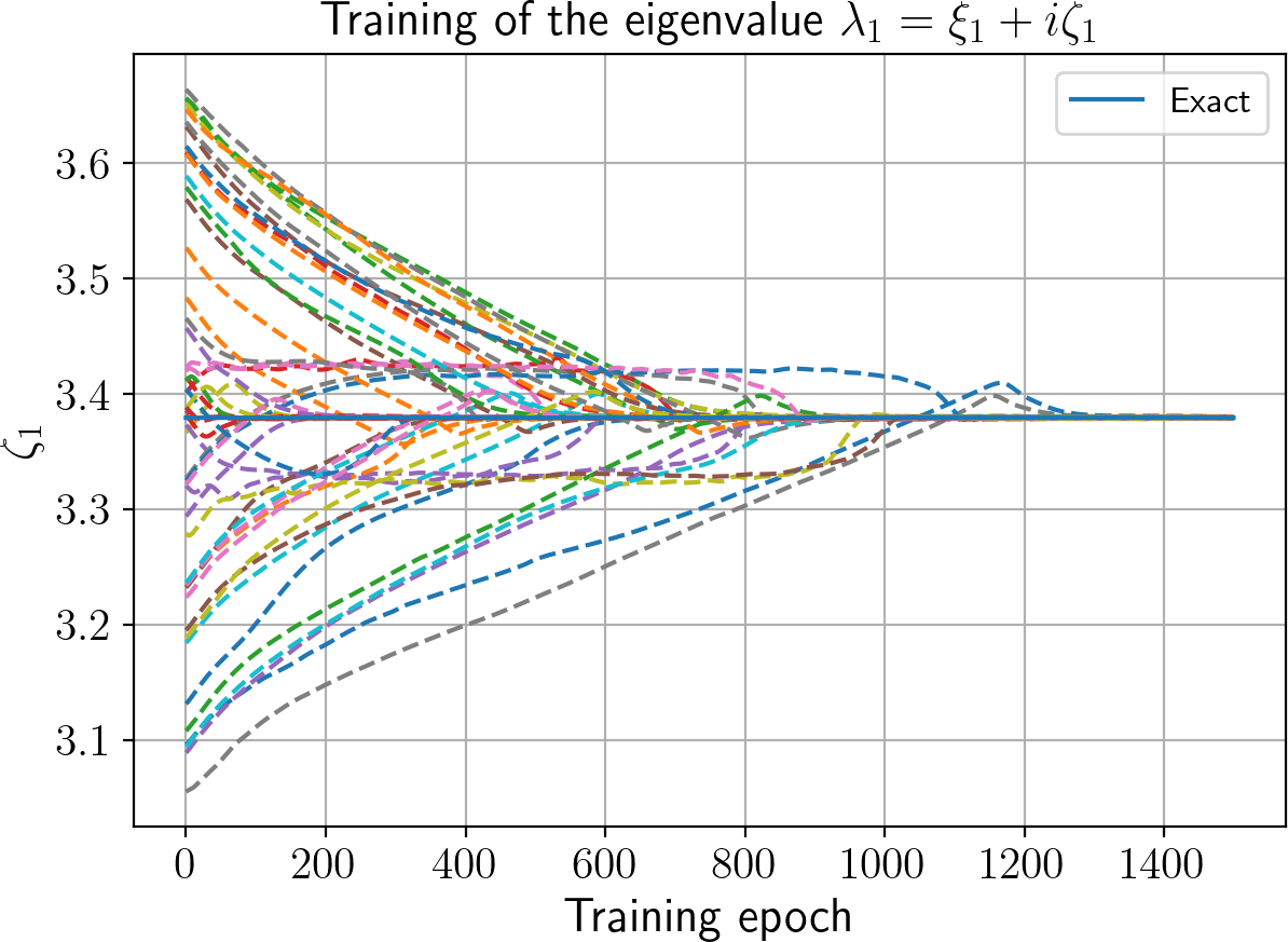
Figure 16: Eigenvalue training progress for Example 4.3 with initialization $\xi\sim\mathcal{U}(\xi_{\text{exact}}-1/2,\xi_{\text{exact}}+1/2)$ and $\zeta\sim\mathcal{U}(\zeta_{\text{exact}}-1/2,\zeta_{\text{exact}}+1/2)$.

We approximate the solution to this example using a feedforward network augmented with knowledge-based function $\Phi(r,\theta;\lambda)=\mathfrak{Re}[r^{\lambda}\Psi_{\lambda}(\theta)]$. Here, $\lambda$ is assumed to be an unknown complex number of the form $\lambda=\xi+i\zeta$. A cutoff function is again used to isolate the behavior of $\Phi$ to a region around the origin. We initialize $\xi$ and $\zeta$ away from their true values in order to demonstrate that the correct behavior may be learned by the augmented feedforward neural network.

Figure 16 shows the training progress of $\lambda$ over 50 trials with $\xi$ and $\zeta$ initialized according to the uniform distributions $\mathcal{U}(\xi_{\text{exact}}-1/2,\xi_{\text{exact}}+1/2)$ and $\mathcal{U}(\zeta_{\text{exact}}-1/2,\zeta_{\text{exact}}+1/2)$, respectively. Remarkably, we observe that the correct eddy behavior is obtained and the values of $\xi$ and $\zeta$ are learned to within about $0.005\%$.

5 Conclusions

We have presented the extended Galerkin neural network framework for approximating a general class of boundary value problems, including those with low-regularity features. This framework utilizes a simple least squares variational formulation alongside an enriched feedforward neural network architecture. We demonstrate that this approach ensures norm equivalence of the induced energy norm with the norm of the solution space and demonstrate the repercussions when this norm equivalence is lost as is the case when standard least squares approaches based on the $L^{2}$ norm are used. Moreover, we have demonstrated the clear advantage of utilizing knowledge-based functions in the network architecture and have shown that xGNN can easily learn these functions.

6 Acknowledgments

J.D. thanks the National Science Foundation Graduate Research Fellowship for its financial support under Grant No. 1644760. This work was performed under the auspices of the U.S. Department of Energy by Lawrence Livermore National Laboratory under Contract DE-AC52-07NA27344; LLNL-JRNL-859911. M.A. gratefully acknowledges the support of National Science Foundation Grant No. DMS-2324364.

Appendix A Knowledge-based functions for Stokes flow

Given a vertex $x^{(i)}$ of $\Omega$ with interior angle $\alpha^{(i)}$, the solution of the Stokes flow in the vicinity of $x^{(i)}$ is may be written into terms of the eigenfunctions of the operator pencil of the Stokes operator [12]. It is simpler to first consider the streamfunction $\psi$, which takes the form

$$\psi(r,\theta)=\sum_{\lambda_{n}}c_{\lambda_{n}}\mathfrak{Re}\left[r^{\lambda_{n}}\Psi_{\lambda_{n}}(\theta)\right],$$

where for $\lambda_{n}\neq 0$, $\Psi_{\lambda_{n}}$ is given by the general form

$$\Psi_{\lambda_{n}}(\theta):=A_{1}\cos((\lambda_{n}-2)\theta)+A_{2}\cos(\lambda_{n}\theta)+A_{3}\sin((\lambda_{n}-2)\theta)+A_{4}\sin(\lambda_{n}\theta).$$

The coefficients $A_{i}$ are chosen to satisfy the boundary conditions. The velocity may be obtained from the streamfunction with the relation $\mathbf{u}=\nabla^{\perp}\psi$ while the pressure may be obtained from the momentum equation $\nabla p=\Delta\mathbf{u}$.

A.1 No-slip boundary conditions

We shall first consider the simple case of no-slip boundary conditions, i.e. $\mathbf{u}\cdot\mathbf{n}=\partial\psi/\partial t=0$. In this case, we have

(44) $$\Psi_{\lambda_{n}}(\theta):=\cos(\lambda_{n}\alpha)\cos((\lambda_{n}-2)\theta)-\cos((\lambda_{n}-2)\alpha)\cos(\lambda_{n}\theta).$$

In the case of complex eigenvalues, the streamfunction produces a sequence of infinitely cascading eddies, a qualitative discussion of which may be found in [16]. To the best of our knowledge, an explicit derivation of the full corresponding eigenfunctions of the eddies for the Stokes velocity and pressure does not exist in the literature. Thus, the purpose of this section is to state the velocities and pressure corresponding to the streamfunction $r^{\lambda_{n}}\Psi_{\lambda_{n}}(\theta)$ assuming complex eigenvalues $\lambda_{n}=\xi_{n}+i\zeta_{n}$. In this case, we have

$$\mathfrak{Re}\left[r^{\lambda_{n}}\Psi_{\lambda_{n}}(\theta)\right]=\mathfrak{Re}[r^{\lambda_{n}}]\mathfrak{Re}[\Psi_{\lambda_{n}}(\theta)]-\mathfrak{Im}[r^{\lambda_{n}}]\mathfrak{Im}[\Psi_{\lambda_{n}}(\theta)]$$

from which the velocity components may be derived:

$$\begin{bmatrix}u_{1}(r,\theta)\\ u_{2}(r,\theta)\end{bmatrix} =\sum_{\lambda_{n}}\begin{bmatrix}\frac{\partial}{\partial r}\mathfrak{Re}[r^{\lambda_{n}}]\mathfrak{Re}[\Psi_{\lambda_{n}}(\theta)]\sin{\theta}+\mathfrak{Re}[r^{\lambda_{n}}]\frac{\partial}{\partial\theta}\mathfrak{Re}[\Psi_{\lambda_{n}}(\theta)]\frac{\cos{\theta}}{r}\\ -\frac{\partial}{\partial r}\mathfrak{Re}[r^{\lambda_{n}}]\mathfrak{Re}[\Psi_{\lambda_{n}}(\theta)]\cos{\theta}+\mathfrak{Re}[r^{\lambda_{n}}]\frac{\partial}{\partial\theta}\mathfrak{Re}[\Psi_{\lambda_{n}}(\theta)]\frac{\sin{\theta}}{r}\end{bmatrix}$$

(45) $$\;\;\;+\sum_{\lambda_{n}}\begin{bmatrix}-\frac{\partial}{\partial r}\mathfrak{Im}[r^{\lambda_{n}}]\mathfrak{Im}[\Psi_{\lambda_{n}}(\theta)]\sin{\theta}-\mathfrak{Im}[r^{\lambda_{n}}]\frac{\partial}{\partial\theta}\mathfrak{Im}[\Psi_{\lambda_{n}}(\theta)]\frac{\cos{\theta}}{r}\\ \frac{\partial}{\partial r}\mathfrak{Im}[r^{\lambda_{n}}]\mathfrak{Im}[\Psi_{\lambda_{n}}(\theta)]\cos{\theta}-\mathfrak{Im}[r^{\lambda_{n}}]\frac{\partial}{\partial\theta}\mathfrak{Im}[\Psi_{\lambda_{n}}(\theta)]\frac{\sin{\theta}}{r}\end{bmatrix}.$$

Here,

$$\mathfrak{Re}[r^{\lambda_{n}}] =r^{\xi_{n}}\cos(\log(r)\zeta_{n}),\;\;\;\mathfrak{Im}[r^{\lambda_{n}}]=r^{\xi_{n}}\sin(\log(r)\zeta_{n})$$

$$\mathfrak{Re}[\Psi_{\lambda_{n}}(\theta)] =\cos(\xi_{n}\alpha^{(i)})\cos((\xi_{n}-2)\theta)\cosh(\zeta_{n}\alpha^{(i)})\cosh(\zeta_{n}\theta)$$

$$\;\;\;+\sin(\xi_{n}\alpha^{(i)})\sin((\xi_{n}-2)\theta)\sinh(\zeta_{n}\alpha^{(i)})\sinh(\zeta_{n}\theta)$$

$$\;\;\;-\cos((\xi_{n}-2)\alpha^{(i)}\cos((\xi_{n}-2)\theta)\cosh(\zeta_{n}\alpha^{(i)})\cosh(\zeta_{n}\theta)$$

$$\;\;\;+\sin((\xi_{n}-2)\alpha^{(i)})\sin(\xi_{n}\theta)\sinh(\zeta_{n}\alpha^{(i)})\sinh(\zeta_{n}\theta)$$

$$\mathfrak{Im}[\Psi_{\lambda_{n}}(\theta)] =-\cos(\xi_{n}\alpha^{(i)})\sin((\xi_{n}-2)\theta)\cosh(\zeta_{n}\alpha^{(i)})\sinh(\zeta_{n}\theta)$$

$$\;\;\;-\sin(\xi_{n}\alpha^{(i)})\cos((\xi_{n}-2)\theta)\sinh(\zeta_{n}\alpha^{(i)})\cosh(\zeta_{n}\theta)$$

$$\;\;\;+\cos((\xi_{n}-2)\alpha^{(i)})\sin(\xi_{n}\theta)\cosh(\zeta_{n}\alpha^{(i)})\sinh(\zeta_{n}\theta)$$

$$\;\;\;+\sin((\xi_{n}-2)\alpha^{(i)})\cos(\xi_{n}\theta)\sinh(\zeta_{n}\alpha^{(i)})\cosh(\zeta_{n}\theta)).$$

We note that (45) has been calculated to exactly satisfy a no-slip condition along $\theta=\pm\alpha^{(i)}$. The transformation $\theta\mapsto\theta-\phi$, $\phi\in\mathbb{R}$ should be taken if necessary depending on specific domain geometry.

Finally, to obtain the pressure corresponding to the streamfunction $\mathfrak{Re}[r^{\lambda_{n}}\Psi_{\lambda_{n}}(\theta)]$, it is straightforward to calculate $\partial p/\partial r$ and $\partial p/\partial\theta$ from the momentum equations in polar coordinates [5]:

(46) $$\begin{dcases}-\left(\frac{\partial^{2}u_{r}}{\partial r^{2}}+\frac{1}{r}\frac{\partial u_{r}}{\partial r}+\frac{1}{r^{2}}\left(\frac{\partial^{2}u_{r}}{\partial\theta^{2}}-2\frac{\partial u_{\theta}}{\partial\theta}-u_{r}\right)\right)+\frac{\partial p}{\partial r}=0\\ -\left(\frac{\partial^{2}u_{\theta}}{\partial r^{2}}+\frac{1}{r}\frac{\partial u_{\theta}}{\partial r}+\frac{1}{r^{2}}\left(\frac{\partial^{2}u_{\theta}}{\partial\theta^{2}}-2\frac{\partial u_{r}}{\partial\theta}-u_{\theta}\right)\right)+\frac{1}{r}\frac{\partial p}{\partial\theta}=0\end{dcases}$$

In (46), $u_{r}$ and $u_{\theta}$ are the radial and azimuthal components of the velocity given by $u_{r}(r,\theta):=r^{-1}\partial\psi/\partial\theta$ and $u_{\theta}(r,\theta):=-\partial\psi/\partial r$, respectively. Integrating $\partial p/\partial r$ and $\partial p/\partial\theta$ and equating constants yields

$$p(r,\theta) =4r^{\xi_{n}-2}\biggl{(}\cos(\xi_{n}\alpha^{(i)})\cosh(\zeta_{n}\alpha^{(i)})\left(-\sin((\xi_{n}-2)\theta)\cosh(\zeta_{n}\theta)A(r)\right.$$

$$\hskip 142.26378pt\left.\left.-\cos((\xi_{n}-2)\theta)\sinh(\zeta_{n}\theta)B(r)\right)+\right.$$

$$\hskip 51.21495pt\left.\sin(\xi_{n}\alpha^{(i)})\sinh(\zeta_{n}\alpha^{(i)})\left(\sin((\xi_{n}-2)\theta)\cosh(\zeta_{n}\theta)B(r)\right.\right.$$

(47) $$\hskip 142.26378pt\left.-\cos((\xi_{n}-2)\theta)\sinh(\zeta_{n}\theta)A(r)\right)\biggr{)},$$

$$A(r) :=-(\xi_{n}-1)\cos(\log(r)\zeta_{n})+\zeta_{n}\sin(\log(r)\zeta_{n})$$

$$B(r) :=\zeta_{n}\cos(\log(r)\zeta_{n})+(\xi_{n}-1)\sin(\log(r)\zeta_{n}).$$

In the special case when $\lambda_{n}\in\mathbb{R}$, we simply take $\zeta_{n}=0$ to arrive at

(48) $$\begin{bmatrix}u_{1}(r,\theta)\\ u_{2}(r,\theta)\\ p(r,\theta)\end{bmatrix} =\sum_{\lambda_{n}}\begin{bmatrix}\lambda_{n}r^{\lambda_{n}-1}\mathfrak{Re}[\Psi_{\lambda_{n}}(\theta)]\sin{\theta}-r^{\lambda_{n}}\frac{\partial}{\partial\theta}\mathfrak{Re}[\Psi_{\lambda_{n}}(\theta)]\cos{\theta}\\ -\lambda_{n}r^{\lambda_{n}-1}\mathfrak{Re}[\Psi_{\lambda_{n}}(\theta)]\cos{\theta}+r^{\lambda_{n}-1}\frac{\partial}{\partial\theta}\mathfrak{Re}[\Psi_{\lambda_{n}}(\theta)]\sin{\theta}\\ 4(\lambda_{n}-1)r^{\lambda_{n}-2}\cos(\lambda_{n}\alpha^{(i)})\sin((\lambda_{n}-2)\theta)\end{bmatrix}.$$

A.2 Homogeneous Dirichlet boundary conditions

For the boundary homogeneous Dirichlet boundary condition $\mathbf{u}=\mathbf{0}$ used in the examples in Section 3, we leave the constants $A_{i}$ as unknowns to be determined during the least squares step (7). In this case, the velocity corresponding to the streamfunction $\mathfrak{Re}[r^{\lambda_{n}}\Psi_{\lambda_{n}}(\theta)]$ consists of four terms:

$$\begin{bmatrix}u_{1}(r,\theta)\\ u_{2}(r,\theta)\end{bmatrix} =\sum_{i=1}^{4}A_{i}\left\{\sum_{\lambda_{n}}\begin{bmatrix}\frac{\partial}{\partial r}\mathfrak{Re}[r^{\lambda_{n}}]\mathfrak{Re}[\Psi_{i,\lambda_{n}}(\theta)]\sin{\theta}+\mathfrak{Re}[r^{\lambda_{n}}]\frac{\partial}{\partial\theta}\mathfrak{Re}[\Psi_{i,\lambda_{n}}(\theta)]\frac{\cos{\theta}}{r}\\ -\frac{\partial}{\partial r}\mathfrak{Re}[r^{\lambda_{n}}]\mathfrak{Re}[\Psi_{i,\lambda_{n}}(\theta)]\cos{\theta}+\mathfrak{Re}[r^{\lambda_{n}}]\frac{\partial}{\partial\theta}\mathfrak{Re}[\Psi_{i,\lambda_{n}}(\theta)]\frac{\sin{\theta}}{r}\end{bmatrix}\right.$$

(49) $$\left.\;\;\;+\sum_{\lambda_{n}}\begin{bmatrix}-\frac{\partial}{\partial r}\mathfrak{Im}[r^{\lambda_{n}}]\mathfrak{Im}[\Psi_{i,\lambda_{n}}(\theta)]\sin{\theta}-\mathfrak{Im}[r^{\lambda_{n}}]\frac{\partial}{\partial\theta}\mathfrak{Im}[\Psi_{i,\lambda_{n}}(\theta)]\frac{\cos{\theta}}{r}\\ \frac{\partial}{\partial r}\mathfrak{Im}[r^{\lambda_{n}}]\mathfrak{Im}[\Psi_{i,\lambda_{n}}(\theta)]\cos{\theta}-\mathfrak{Im}[r^{\lambda_{n}}]\frac{\partial}{\partial\theta}\mathfrak{Im}[\Psi_{i,\lambda_{n}}(\theta)]\frac{\sin{\theta}}{r}\end{bmatrix}\right\}.$$

For ease of notation, we use $\Psi_{i,\lambda_{n}}$ to denote the four component eigenfunctions

$$\Psi_{1,\lambda_{n}}(\theta) =\cos((\lambda_{n}-2)\theta),\;\;\;\Psi_{2,\lambda_{n}}(\theta)=\cos(\lambda_{n}\theta),$$

$$\Psi_{3,\lambda_{n}}(\theta) =\sin((\lambda_{n}-2)\theta),\;\;\;\;\Psi_{4,\lambda_{n}}(\theta)=\sin(\lambda_{n}\theta).$$

The real and complex components of $\Psi_{i,\lambda_{n}}$ are given by

$$\mathfrak{Re}[\Psi_{1,\lambda_{n}}(\theta)] =\cos((\xi_{n}-2)\theta)\cosh(\zeta_{n}\theta),\;\;\;\mathfrak{Im}[\Psi_{1,\lambda_{n}}(\theta)]=-\sin((\xi_{n}-2)\theta)\sinh(\zeta_{n}\theta),$$

$$\mathfrak{Re}[\Psi_{2,\lambda_{n}}(\theta)] =\cos(\xi_{n}\theta)\cosh(\zeta_{n}\theta),\;\;\;\;\;\;\;\;\;\;\;\;\mathfrak{Im}[\Psi_{2,\lambda_{n}}(\theta)]=-\sin(\xi_{n}\theta)\sinh(\zeta_{n}\theta),$$

$$\mathfrak{Re}[\Psi_{3,\lambda_{n}}(\theta)] =\sin((\xi_{n}-2)\theta)\cosh(\zeta_{n}\theta),\;\;\;\mathfrak{Im}[\Psi_{3,\lambda_{n}}(\theta)]=\cos((\xi_{n}-2)\theta)\sinh(\zeta_{n}\theta),$$

$$\mathfrak{Re}[\Psi_{4,\lambda_{n}}(\theta)] =\sin(\xi_{n}\theta)\cosh(\zeta_{n}\theta),\;\;\;\;\;\;\;\;\;\;\;\;\mathfrak{Im}[\Psi_{4,\lambda_{n}}(\theta)]=\cos(\xi_{n}\theta)\sinh(\zeta_{n}\theta).$$

The pressure corresponding to $\mathfrak{Re}[r^{\lambda_{n}}\Psi_{\lambda_{n}}(\theta)]$ is given by

(50) $$p(r,\theta)=\sum_{i=1}^{4}A_{i}P_{i,\lambda_{n}}(r,\theta),$$

where the four component eigenfunctions $P_{i,\lambda_{n}}$ are

$$P_{1,\lambda_{n}}(r,\theta) =4r^{\xi_{n}-2}\left(\sin((\xi_{n}-2)\theta)\cosh(\zeta_{n}\theta)A(r)+\cos((\xi_{n}-2)\theta)\sinh(\zeta_{n}\theta)B(r)\right)$$

$$P_{3,\lambda_{n}}(r,\theta) =4r^{\xi_{n}-2}\left(-\cos((\xi_{n}-2)\theta)\cosh(\zeta_{n}\theta)A(r)+\sin((\xi_{n}-2)\theta)\sinh(\zeta_{n}\theta)B(r)\right)$$

with $P_{2,\lambda_{n}}(r,\theta)=P_{4,\lambda_{n}}(r,\theta)=0$ and $A(r)$, $B(r)$ as in (47).

Appendix B Hyperparameters for numerical examples

Parameter	$\mathbf{n}^{(i)}$	$L_{i}$	$\sigma$	learning rate	$\delta$
	$20\cdot 2^{i-1}$	1	$\tanh((1+\frac{i}{4})t)$	$0.001/1.1^{i-1}$	$10^{3}$

Table 1: General hyperparameters for learning $\varphi_{i}^{NN}$ in all examples. Any example-specific deviations from this configuration are provided in Tables B.1-B.5.

B.1 Example 2.3

4mm

training data	tensor-product Gauss-Legendre $128\times 128$ in $\Omega$; left Riemann sum 256 on $\partial\Omega$
$\delta$	Variable. See Example 2.3 for details.

B.2 Examples 3.2-3.3

0mm

$n_{\lambda}^{(i)}$	$\mathbf{n}^{(i)}/2$
$\Phi$	$r^{\lambda}\sin(\lambda\theta)$
$\lambda$2	$2j/3$
training data	tensor-product Gauss-Legendre $128\times 128$ in each square quadrant of $\Omega$; Gauss-Legendre 128 on each edge of $\partial\Omega$

B.3 Example 3.5

0mm

$n_{\lambda}^{(i)}$	$5i$ in non-convex corners; $1$ in convex corner
$\Phi$	Equations (A.2) and (50)
training data	tensor-product Gauss-Legendre $128\times 128$ in each square quadrant of channel and rectangle enclosing triangular cavity of $\Omega$; Gauss-Legendre 128 on each edge of $\partial\Omega$

B.4 Example 4.1

0mm

$n_{\lambda}^{(i)}$	1
$\Phi$	$r^{\lambda}\sin(\lambda\theta)$
training data	tensor-product Gauss-Legendre $128\times 128$ in each square quadrant of $\Omega$; Gauss-Legendre 128 on each edge of $\partial\Omega$

B.5 Examples 4.2-4.3

0mm

$\mathbf{n}^{(i)}$ & $n^{(i)}_{\lambda}$	$20\cdot 1.9^{i-1}$ & 1
$\Phi$	Equation (48) in 4.2; (45) and (47) in 4.3
training data	tensor-product Gauss-Legendre $128\times 128$ in each square quadrant of $\Omega$; Gauss-Legendre 128 on each edge of $\partial\Omega$
learning rate	$0.003/1.1^{i-1}$

References

- [1] M. Ainsworth and J. Dong, Galerkin neural networks: A framework for approximating variational equations with error control, SIAM Journal on Scientific Computing, 43 (2021), pp. A2474–A2501.
- [2] M. Ainsworth and J. Dong, Galerkin neural network approximation of singularly-perturbed elliptic systems, Computer Methods in Applied Mechanics and Engineering, 402 (2022), p. 115169.
- [3] A. Arzani, K. W. Cassel, and R. M. D’Souza, Theory-guided physics-informed neural networks for boundary layer problems with singular perturbation, Journal of Computational Physics, 473 (2023), p. 111768.
- [4] Y. Bar-Sinai, S. Hoyer, J. Hickey, and M. P. Brenner, Learning data-driven discretizations for partial differential equations, Proceedings of the National Academy of Sciences, 116 (2019), pp. 15344–15349.
- [5] G. K. Batchelor, An introduction to fluid dynamics, Cambridge university press, 1967.
- [6] H. Blum, R. Rannacher, and R. Leis, On the boundary value problem of the biharmonic operator on domains with angular corners, Mathematical Methods in the Applied Sciences, 2 (1980), pp. 556–581.
- [7] P. B. Bochev and M. D. Gunzburger, Least-squares finite element methods, vol. 166, Springer Science & Business Media, 2009.
- [8] M. Dissanayake and N. Phan-Thien, Neural-network-based approximations for solving partial differential equations, Communications in Numerical Methods in Engineering, 10 (1994), pp. 195–201.
- [9] B. Guo and C. Schwab, Analytic regularity of stokes flow on polygonal domains in countably weighted sobolev spaces, Journal of Computational and Applied Mathematics, 190 (2006), pp. 487–519.
- [10] K. Hornik, M. Stinchcombe, and H. White, Universal approximation of an unknown mapping and its derivatives using multilayer feedforward networks, Neural networks, 3 (1990), pp. 551–560.
- [11] V. A. Kondrat’ev, Boundary value problems for elliptic equations in domains with conical or angular points, Trudy Moskovskogo Matematicheskogo Obshchestva, 16 (1967), pp. 209–292.
- [12] V. Kozlov, V. G. Maz’ya, and J. Rossmann, Spectral problems associated with corner singularities of solutions to elliptic equations, American Mathematical Soc., 2001.
- [13] I. E. Lagaris, A. Likas, and D. I. Fotiadis, Artificial neural networks for solving ordinary and partial differential equations, IEEE transactions on neural networks, 9 (1998), pp. 987–1000.
- [14] Z. Li, N. B. Kovachki, K. Azizzadenesheli, K. Bhattacharya, A. Stuart, A. Anandkumar, et al., Fourier neural operator for parametric partial differential equations, in International Conference on Learning Representations, 2020.
- [15] L. Lu, P. Jin, G. Pang, Z. Zhang, and G. E. Karniadakis, Learning nonlinear operators via deeponet based on the universal approximation theorem of operators, Nature Machine Intelligence, 3 (2021), pp. 218–229, https://doi.org/10.1038/s42256-021-00302-5.
- [16] H. K. Moffatt, Viscous and resistive eddies near a sharp corner, Journal of Fluid Mechanics, 18 (1964), pp. 1–18.
- [17] S. Pakravan, P. A. Mistani, M. A. Aragon-Calvo, and F. Gibou, Solving inverse-pde problems with physics-aware neural networks, Journal of Computational Physics, 440 (2021), p. 110414.
- [18] M. Raissi, P. Perdikaris, and G. E. Karniadakis, Physics-informed neural networks: A deep learning framework for solving forward and inverse problems involving nonlinear partial differential equations, Journal of Computational physics, 378 (2019), pp. 686–707.
- [19] S. A. Sauter and C. Schwab, Boundary element methods, Springer, 2011.
- [20] C. Schwab, p-and hp-finite element methods: Theory and applications in solid and fluid mechanics, Clarendon Press, 1998.
- [21] T. Strouboulis, K. Copps, and I. Babuška, The generalized finite element method, Computer methods in applied mechanics and engineering, 190 (2001), pp. 4081–4193.
- [22] N. Sukumar, N. Moës, B. Moran, and T. Belytschko, Extended finite element method for three-dimensional crack modelling, International journal for numerical methods in engineering, 48 (2000), pp. 1549–1570.
- [23] J. Yang, K. Mittal, T. Dzanic, S. Petrides, B. Keith, B. Petersen, D. Faissol, and R. Anderson, Multi-agent reinforcement learning for adaptive mesh refinement, arXiv preprint arXiv:2211.00801, (2022).
- [24] Y. Zang, G. Bao, X. Ye, and H. Zhou, Weak adversarial networks for high-dimensional partial differential equations, Journal of Computational Physics, 411 (2020), p. 109409.