Convection and the Core $g$-mode in Proto-Compact Stars – A detailed analysis

Abstract

We present a detailed analysis of the dynamics of proto-compact star (PCS) convection and the core ${}^{2}\!g_{1}$-mode in core-collapse supernovae based on general relativistic 2D and 3D neutrino hydrodynamics simulations. Based on 2D simulations, we derive a mode relation for the core $g$-mode frequency in terms of PCS and equation of state parameters, and discuss its limits of accuracy. This relation may prove useful for parameter inference from future supernova gravitational wave (GW) signals if the core $g$-mode or an emission gap at the avoided crossing with the fundamental mode can be detected. The current 3D simulation does not show GW emission from the core $g$-mode due to less power in high-frequency convective motions to excite the mode, however. Analysing the dynamics of PCS convection in 3D, we find that simple scaling laws for convective velocity from mixing-length theory (MLT) do not apply. Energy and lepton number transport is instead governed by a more complex balance between neutrino fluxes and turbulent fluxes that results in roughly uniform rates of change of entropy and lepton number in the PCS convection zone. Electron fraction and enthalpy contrasts in PCS convection are not well captured by the MLT gradient approximation. We find distinctly different spectra for the turbulent kinetic energy and turbulent fluctuations in the electron fraction, which scale approximately as $l^{-1}$ without a downturn at low $l$. We suggest that the different turbulence spectrum of the electron fraction is naturally expected for a passive scalar quantity.

1 Introduction

Ordinary core-collapse supernovae (CCSNe) with explosion energies of $\mathord{\sim}10^{51}\,\mathrm{erg}$ explode via the delayed neutrino-driven mechanism (Colgate et al., 1961). In the neutrino-driven paradigm the shock wave formed during core bounce stalls at a radius of about $100\,\mathrm{km}-200\,\mathrm{km}$, and gets revitalised by partial re-absorption of neutrinos emitted from the proto-compact star (PCS). This leads to the expulsion of outer layers of the star (Janka et al., 2016; Müller, 2020; Burrows & Vartanyan, 2021).

Multi-dimensional effects are critical for the success of neutrino-driven explosions and highly relevant to observations as they imprint characteristic signatures on the neutrino and gravitational wave signals of the supernova core (Müller, 2019a; Abdikamalov et al., 2022). Neutrino heating drives convective overturn in the gain region behind the supernova shock (Herant et al., 1992; Herant et al., 1994; Burrows et al., 1995; Janka & Mueller, 1996). In addition, large-scale shock oscillations, i.e., the standing accretion shock instability (SASI) can develop due to a vortical-acoustic feedback cycle (Blondin et al., 2003; Guilet & Foglizzo, 2012). Convection develops inside the newly formed PCS after the collapse of the iron core between radii of $10\,\mathrm{km}\mathord{\lesssim}r\mathord{\lesssim}25\,\mathrm{km}$ due to energy and lepton-number losses at the PCS surface. Early theoretical considerations suggested that convective instabilities beneath the neutrinosphere play a vital role in CCSN dynamics (Epstein, 1979; Bruenn et al., 1979; Livio et al., 1980). As PCS convection significantly affects neutrino luminosities and mean energies, it has a potentially relevant impact on the neutrino heating conditions and hence the conditions for explosion (Keil et al., 1996), but later studies by Dessart et al. (2006); Buras et al. (2006) have shifted the focus away from the dynamical role of PCS convection in the explosion mechanism. As PCS convection efficiently transports energy and lepton number out of the PCS core, it does, however, affect the observable neutrino signal and the PCS cooling evolution (Roberts et al., 2012; Mirizzi et al., 2016; Pascal et al., 2022).

PCS convection also contributes to gravitational-wave (GW) emission from CCSNe. Along with aspherical fluid motions in the gain region, it excites oscillation of the quadrupolar $f$/$g$ surface oscillation mode that constitutes the most prominent feature in the supernova GW signal. It may even be a GW source in its own right (Murphy et al., 2009; Müller et al., 2013; Andresen et al., 2017; Morozova et al., 2018; Radice et al., 2019; Mezzacappa et al., 2020; Vartanyan et al., 2023). More recently, the ${}^{2}\!g_{1}$-mode in the PCS core has received attention. Its primary forcing mechanism is PCS convection. This core $g$-mode has been found in 2D simulations (Cerdá-Durán et al., 2013; Kawahara et al., 2018; Torres-Forné et al., 2019a; Jakobus et al., 2023) and recently also in 3D (Vartanyan et al., 2023), and is of interest as a more direct probe of the high-density equation of state than the surface $f$/$g$-mode. As demonstrated by Jakobus et al. (2023), the ${}^{2}\!g_{1}$-mode is sensitive to the speed of sound at around twice saturation density. The conditions for the excitation of the core ${}^{2}\!g_{1}$-mode are, however, still less clear than for the surface $f$/$g$-mode. Moreover, the relation of the ${}^{2}\!g_{1}$-mode to the physical parameters of the PCS are not yet as well understood as for the surface $f$/$g$-mode. For the surface $f$/$g$-mode, various physically motivated fitting formulas have been proposed to relate the mode frequency to the PCS mass, radius, and surface temperature (Müller et al., 2013; Morozova et al., 2018; Torres-Forné et al., 2019a; Sotani et al., 2021; Mori et al., 2023). As of yet, little effort has been made to find analytically motivated relations for the ${}^{2}\!g_{1}$-mode. In this study, we aim for a simple “semi-analytic” estimate of the core $g$-mode, analogously to the analysis done for the surface quadrupolar $g$-mode in Müller et al. (2013). This could potentially enable parameter estimation of PNS core properties and equation of state (EoS) parameters based on the prospective GW signal from the quadrupolar core $g$-mode.

Related to the GW emission and mode excitation by PCS convection, there are also open questions about the dynamics of the convective flow. In the case of convection in the gain region, the saturation of turbulent kinetic energy (Müller, 2020) and the relation between turbulent kinetic energy and the emission of GWs via excitation of the surface $f/g$-mode (Müller, 2017; Powell & Müller, 2019; Radice et al., 2019) have been investigated extensively. The impact of dimensionality on convection in the gain region has also been thoroughly investigated (e.g., Hanke et al., 2012; Dolence et al., 2013; Couch & Ott, 2013), identifying critical differences in the dynamics of neutrino-driven convection in two (2D) and three dimensions (3D) due to the inverse turbulent cascade in 2D (Kraichnan, 1967). Empirically, it has been found that GW emission due to the excitation of the surface $f/g$-mode by convection in the gain region is weaker in 2D, which has been attributed to smaller terminal downflow velocities and less high-frequency variability in the downflows (Andresen et al., 2017). By and large, these issues have been less well explored for PCS convection, although the phenomenology of PCS convection across the progenitor mass range has recently been studied by Nagakura et al. (2020).

One of the more puzzling aspects of PCS convection is the lepton-number emission self-sustained asymmetry (LESA) that has been found in many 3D simulations (Tamborra et al., 2014; Vartanyan et al., 2019; O’Connor & Couch, 2018; Powell & Müller, 2019; Janka et al., 2016; Glas et al., 2019; Vartanyan et al., 2018; Nagakura et al., 2020) and still remains incompletely understood. In LESA, the neutrino emission develops a dipolar asymmetry several hundreds of milliseconds after core-bounce. The hemispheric luminosity difference of $\nu_{e}$ and $\overline{\nu}_{e}$ neutrinos can amount to tens of percent. Different from the initial proposition of a feedback mechanism between accretion and PCS convection (Tamborra et al., 2014), the mechanism responsible for LESA may operate entirely within the PCS convective region (Glas et al., 2019). Janka et al. (2016) identified complex flow dynamics in LESA due to the sensitivity of the Ledoux criterion to the (negative) radial electron fraction gradient $\mathrm{d}Y_{\!\mathrm{e}}/\mathrm{d}r$, which can become stabilising depending on the thermodynamic derivative$\left(\partial\rho/\partial Y_{\!\mathrm{e}}\right)_{P,s}$. This can inhibit convection in certain directions and in turn lead to less effective transport of lepton number upwards from the lepton-rich inner core, and in conjunction with neutrino diffusion a positive feedback cycle can be envisaged that gives rise to a sustained global asymmetry in the election fraction. To explain the low-mode nature of LESA, the study by Glas et al. (2019) drew an analogy between the excitation of harmonics of different orders in thermally unstable spherical shells according to Chandrasekhar’s linear theory of thermal instability in spherical shells (Chandrasekhar & Gillis, 1962). Building further on this, Powell & Müller (2019) suggested LESA not to be a new instability but instead a manifestation of convection, but with a non-Kolmogorov velocity spectrum due to the presence of a stabilising $Y_{\mathrm{e}}$-gradient in the middle of the convection zone. In this paper, we further address these current topics in PCS convection. Following our recent study of GW emission from the core $g$-mode (Jakobus et al., 2023), we conduct 2D and 3D simulations with the relativistic neutrino hydrodynamics code CoCoNuT-FMT (Müller et al., 2010; Müller & Janka, 2015) for massive zero-metallicity progenitor stars of $35\mathrm{M}_{\odot}$ and $85\mathrm{M}_{\odot}$ with strong PCS convection. Based on these simulations, we shall investigate the following questions:

1. What determines the trajectory of the core $g$-mode frequency, and can this frequency be related to PCS properties?

2. How does the amplitude of the core $g$-mode signal depend on dimensionality?

3. What determines the convective velocities the PCS convection zone and how well are they described by mixing-length theory?

4. What determines the spectrum of $Y_{\mathrm{e}}$-fluctuations in the PCS convection zone (and possibly the dominance of the dipole in LESA)?

The structure of this paper is as follows: In Section 2, we give an overview of the numerical methods, progenitor setup and the equation of state. In Section 3 we analyse the GW signals of our models. We discuss the GW signals of our 2D and 3D simulations, and then develop approximations for the frequency trajectory of the core $g$-mode. In Section 4, we investigate the properties of the PCS convection zone. We briefly discuss basic explosion properties, analyse the structure of turbulent motion, present turbulent kinetic energies in the PCS convection zone for both 2D and 3D, temporal fluctuations in PCS convection, and the efficiency of turbulent convection. We then discuss to what extent the turbulent convective velocities are captured by balancing principles and mixing-length theory (MLT). Finally, we address the spectrum of velocity and passive sclars in the PCS convection zones. A summary of our findings and conclusions are presented in Section 5.

2 Methods

We use the neutrino-hydrodynamic code CoCoNuT-FMT for our 2D and 3D CCSN simulations. The equations of hydrodynamics are solved with a general relativistic finite-volume based solver (Müller et al., 2010). For the neutrino-transport, we use the fast multigroup transport method of Müller (2015). For computational efficiency, the innermost zones are treated in spherical symmetry. In order to capture the entire PCS convection zone in 2D or 3D, we decrease the inner boundary of the spherical core to $3.1\,\mathrm{km}$ before PCS convection develops.

At high densities, we consider two different nuclear equations of state. In one set, we employ the CMF equation of state with a first-order nuclear liquid-vapour phase transition at densities $\mathord{\sim}\rho_{0}$, a second (weak) first-order phase transition due to chiral symmetry restoration at $\mathord{\sim}4\mathord{\times}\rho_{0}$ with a critical endpoint at $T_{\mathrm{CeP}}=15\,\mathrm{MeV}$, and a smooth transition to quark matter at higher densities (Motornenko et al., 2020). We also consider one model with the SFHx EoS (Steiner et al., 2013). The high-density EoS is denoted by a model suffix _CMF or _SFHx, respectively. At low densities, the equation of state includes 20 species of non-interacting nucleons and nuclei, electrons, positrons, and photons. Nuclear reactions are treated by the flashing scheme of Rampp & Janka (2000). At a temperature above $0.5\,\mathrm{MeV}$, nuclear statistical equilibrium is assumed.

As in Jakobus et al. (2023), we use two zero-metallicity progenitors of $35\,\mathrm{M}_{\odot}$ and $85\,\mathrm{M}_{\odot}$, named z35 and z85, (Heger & Woosley, 2010), and additionally simulate a zero-metallicity $85\,\mathrm{M}_{\odot}$ progenitor in 3D (utilising the CMF EoS); all progenitors are calculated with the stellar evolution code Kepler (Weaver et al., 1978).

Gravitational wave signals are computed with the time-integrated quadrupole formula with general relativistic corrections (Müller et al., 2013).

3 Gravitational Wave Emission

In this section, we compare GW spectrograms of the 2D and 3D simulations of the $85\,\mathrm{M}_{\odot}$ progenitor with the CMF EoS. Subsequently, we develop approximations for the core $g$-mode frequency based on the GW spectrograms of the $85\,\mathrm{M}_{\odot}$ and $35\,\mathrm{M}_{\odot}$ progenitors simulated in 2D in Jakobus et al. (2023), with the CMF and SFHx EoS (Motornenko et al., 2020; Steiner et al., 2013).

3.1 Comparison of Spectrograms in 2D and 3D

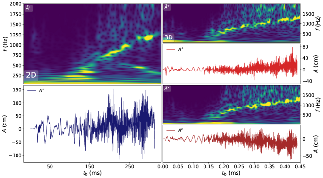
Figure 1: GW spectrograms and amplitudes for models z85 for 2D (left) and 3D (right). Plus and cross amplitudes are evaluated for an observer in the equatorial plane. The CMF-EoS is employed in both runs. Note, that the 2D run exhibits a higher maximum scale for the amplitude $|\tilde{A}|^{+}$ as GW amplitudes are generally increased in 2D compared to 3D. The 2D model exhibits the distinct second frequency band from the ${}^{2}\!g_{1}$-mode, which branches of the dominant band after a few hundred milliseconds. The core $g$-mode signal is absent in 3D.

Figure 1 shows GW spectrograms obtained with the Morlet wavelet transform (Morlet et al., 1982), together with the signal amplitude. The GW signal for the 2D run of model z85_CMF is shown in the left column (plus polarisation only), and results (for both the plus and cross polarisation) from the corresponding 3D run are shown on the right. The signals are shown for an observer at the equator at $(\theta,\phi)=(90\degree,90\degree)$.

The 2D run exhibits significantly larger GW amplitudes with $A^{\!+}>150\,\mathrm{cm}$, compared to $A^{\,+}\lesssim 80\,\mathrm{cm}$ in the 3D model. This is a known feature and has been explained by smaller convective structures, slower overturn velocities, and less impulsive forcing on the PCS surface in 3D (Mueller & Janka, 1997; Müller et al., 2012a; Andresen et al., 2017). Nonetheless, the amplitudes of the 3D model are very high for both the plus and cross components (up to $A^{\!+}\mathord{\sim}80\,\mathrm{cm}$). This can be compared to the results of Powell et al. (2021), who simulated the same progenitor with the SFHx-EoS and found smaller amplitudes of the order $A^{\!+}\mathord{\sim}25\,\mathrm{cm}$. In the initial phase, the spectrograms of the 2D and 3D simulations are very similar. Both models display low-frequency GW emission at around $100\,\mathrm{Hz}$. This is due primarily to the presence of prompt convection and early SASI activity (Marek et al., 2009; Murphy et al., 2009; Yakunin et al., 2010; Müller et al., 2013). The 2D model shows stronger low-frequency activity than the 3D model throughout the simulation. Later on, as emission moves to higher frequencies, the dominant $f/g$-mode emission band emerges in both models, starting at around $\mathord{\sim}300\,\mathrm{Hz}$ and reaching frequencies above $1400\,\mathrm{Hz}$ in 3D. In 2D, the evolution is cut off at $\mathord{\sim}1250\,\mathrm{Hz}$ because a black hole forms early on. We note that the $f/g$-mode frequency increases slightly faster in the 2D simulation. One key difference between the spectrograms of both models is that the core $g$-mode is absent in 3D. This particular ${}^{2}\!g_{1}$ mode is typically located in deep regions of the PCS at radii $5\,\mathrm{km}\lesssim R\lesssim 15\,\mathrm{km}$. Previous 2D studies have identified this mode (Cerdá-Durán et al., 2013; Kawahara et al., 2018; Torres-Forné et al., 2019b; Jakobus et al., 2023) and linked to the speed of sound (Jakobus et al., 2023); more recently, it has also been identified in 3D (Vartanyan et al., 2023). GW emission from the core $g$-mode is thus a less robust feature than the the signal from the $f/g$-mode. This does not imply that the core $g$-mode is a 2D artefact. Its absence in the current simulation may be compounded by stochastic model variations. More high-resolution 3D models are required to decide whether and when it appears and whether is potentially detectable.

3.2 Core $g$-mode frequency relation

If the GW signal from the core $g$-mode is present and detectable under certain circumstances, it is important to connect the mode frequency to physical parameters of the PCS and the EoS. Even if the core $g$-mode is not present or only visible in the spectrogram for a shorter time, the avoided crossing with the surface $f/g$-mode may be a more robust feature (Morozova et al., 2018; Sotani & Takiwaki, 2020; Vartanyan et al., 2023) that can potentially be used for inferring PCS or EoS parameters. In this section, we use the three 2D models z35:CMF, z85:SFHx, and z85:CMF from Jakobus et al. (2023) to develop and assess analytic approximations for the core $g$-mode frequency in terms of EoS and PCS parameters.

For approximating the mode frequency $f_{{}^{2}g_{1}}$ analytically, we note that the frequency of low-order $g$-modes living in a convectively stable region often scales well with the maximum of the Brunt-Väisälä frequency , i.e., $f_{{}^{2}g_{1}}\propto\omega_{\mathrm{BV}}$, with a proportionality factor of order unity. The maximum of the Brunt-Väisälä frequency is located at the edge of the PCS core and associated with a recognisable entropy step between the core and the PCS convection zone. For the first few hundred milliseconds after bounce, the entropy step established by the early propagation of the shock will not change substantially due to efficient neutrino trapping, and we can therefore assume to first order that the location of the step $M_{\mathrm{fix}}$ in mass coordinate remains constant (though perhaps somewhat EoS-dependent), and that the entropy and electron fraction gradients at this point also remain roughly constant. This approximation will, of course, eventually break down at later post-bounce times.

The task is then to approximate the maximum of $\omega_{\mathrm{BV}}$, which can be written in general relativity as (Jakobus et al., 2023),

$$\omega_{\mathrm{BV}}^{2} =\underbrace{\derivative{\alpha}{r}\frac{\alpha}{h\phi^{4}}}_{\mathrm{``effective\,rel.\,acc.^{\prime\prime}}}\underbrace{\frac{1}{\rho c_{\mathrm{s}}^{2}}\left\{\left(\partialderivative{P}{s}\right)_{\rho,Y_{\mathrm{e}}}\derivative{s}{r}+\left(\partialderivative{P}{Y_{\mathrm{e}}}\right)_{\rho,s}\derivative{Y_{\mathrm{e}}}{r}\right\}}_{\mathrm{``EoS\,\,factors^{\prime\prime}}},$$ (1)

for a conformally flat metric. Here $r$ is the radial coordinate, $\alpha$ is the lapse function, $\phi$ is the conformal factor, $c_{\mathrm{s}}$ is the sound speed, $P$ is the pressure, $s$ is the specific entropy, $Y_{\mathrm{e}}$ is the electron fraction, and $h$ is the relativistic enthalpy, which is defined in terms of $P$, the density $\rho$ and the specific internal energy $\epsilon$ as $h=1+\epsilon+P/\rho$. The right-hand side of Equation (1) can conveniently be split into an effective relativistic acceleration term (as a generalisation of the Newtonian gravitational accleration) and factors that depend on the the EoS and radial derivatives of thermodynamics quantities (“EoS factors”).

To this end, we seek suitable approximations for the metric functions $\phi$ and $\alpha$, and the derivative $\mathrm{d}\alpha/\mathrm{d}r$, and for the radial gradient of the entropy $\mathrm{d}s/\mathrm{d}r$ at the edge of the core which determines the stiffness of the convectively stable region. This enables us to formulate an an EoS-dependent mode relation, which could constrain the EoS at high densities via the thermodynamic terms that appears in the Brunt-Väisälä frequency. Throughout the following calculations, we will use geometric units for metric quantities.

3.2.1 Metric terms

To approximate the metric function $\alpha$ in the “effective relativistic acceleration” $c_{\mathrm{gr}}$ (see prefactor in Eq. 1), we work in the Newtonian limit (where $\alpha\approx 1+\Phi$ in terms of the Newtonian potential $\Phi$) and include contributions to the potential from the mass $M_{\mathrm{mode}}$ inside the boundary between the core and the PCS convection zone and the remaining neutron star mass outside. We show the detailed calculation for the approximate lapse function in the Appendix A and only quote the result,

$$\alpha\approx 1-G\left(\frac{M_{\mathrm{mode}}}{r_{\mathrm{mode}}}-\frac{M_{\mathrm{NS}}-M_{\mathrm{mode}}}{\langle r\rangle}\right)+\mathcal{O}(r^{-2}),$$ (2)

where $r_{\mathrm{mode}}$ is the radius of where the core $g$-mode is located, $M_{\mathrm{NS}}$ is the baryonic mass of the PCS. The coefficient $c_{\mathrm{eff}}$ is set to $c_{\mathrm{eff}}=0.5$. Finally, $\langle r\rangle$ is an “effective” radius for the PCS material outside the core,

$$\langle r\rangle\equiv c_{\mathrm{eff}}(R_{\mathrm{NS}}+R_{\mathrm{mode}}).$$ (3)

Building on this approximation for $\alpha$, we proceed to estimate the entire effective relativistic acceleration term in Equation (1). It is useful to factor our the term $r^{-2}$, so that we can approximate the more slowly varying quantity,

$$c_{\mathrm{gr}}~{}\equiv~{}\left[{\mathrm{d}\alpha}/{\mathrm{d}r}\!\cdot r^{2}\!{\alpha}/{(h\phi^{4})}\right]^{1/2}.$$ (4)

Hence, $\omega_{\mathrm{BV}}^{2}$ becomes,

$$\omega_{\mathrm{BV}}=c_{\mathrm{gr}}\sqrt{\frac{1}{r^{2}\rho c_{\mathrm{s}}^{2}}\left\{\left(\partialderivative{P}{s}\right)_{\rho,Y_{\mathrm{e}}}\derivative{s}{r}+\left(\partialderivative{P}{Y_{\mathrm{e}}}\right)_{\rho,s}\derivative{Y_{\mathrm{e}}}{r}\right\}},$$ (5)

Separating the factor $r^{-2}$ has the added benefit that we can later absorb the term $r^{2}\rho$ inside the square root by rewriting the radial thermodynamic derivatives as derivatives with respect to enclosed mass $m$.

To find an expression for $c_{\mathrm{gr}}$, we note that the lapse function $\alpha$ and conformal factor $\phi$ within the PCS approximately conform to the relation $\alpha\phi^{2}~{}\approx~{}1$ (Müller et al., 2013). Since the thermodynamic structure is related to the gravitational potential in hydrostatic equilibrium, we can also empirically relate the enthalpy $h$ to the conformal factor $\phi$ as $h\approx\phi$. In addition, we use the approximation $\mathrm{d}\alpha/\mathrm{d}r\approx Gmh/(r\phi^{2})^{2}$, where $r\phi^{2}$ is the circumferential radius. The factor $h$ provides a crude correction factor for converting $m$ into the gravitational mass of the PCS core.

Figure 2 shows our fits for the individual terms in the relativistic prefactor $c_{\mathrm{gr}}$ for the 2D model z85:CMF. The shaded regions depict fit values for different fixed mass coordinates $M_{\mathrm{fix}}$. The dashed red line represents the exact value at the peak of the Brunt-Väisälä frequency; the dashed black line shows our analytic estimate evaluated at the mass coordinate corresponding to the peak of the Brunt-Väisälä frequency. Note that the error can not be more accurate than the approximation evaluated at the peak of the Brunt-Väisälä frequency. The two error sources are thus the approximations itself, and the assumption that the mass coordinate, $M_{\mathrm{fix}}$, of the entropy step is approximately constant. The approximation tracks the lapse function $\sqrt{\alpha}$ with a small offset, but the overall trend aligns well. Early on, the approximation to the derivative $\left(\mathrm{d}\alpha/\mathrm{d}r\right)^{1/2}$ matches very well, whereas it deviates by $\mathord{\sim}10\%$ at later times. At early times, $\mathrm{d}\alpha/\mathrm{d}r$ is quite sensitive to the choice of the fixed mass shell, however, later on, the error arises from the approximation of the derivative of the metric function $\mathrm{d}\alpha/\mathrm{d}r$, and not from the choice of the fixed mass shell (see red line versus black line). Nevertheless, it is clear that a choice of $M_{\mathrm{fix}}\mathord{\sim}0.7,\mathrm{M}_{\odot}$ provides the best fit. Our approximation of the enthalpy $\sqrt{h}$ is very accurate, with errors below $\mathord{\sim}3\%$. The conformal factor $\phi$ has an acceptable error of $\mathord{\sim}6\%$.

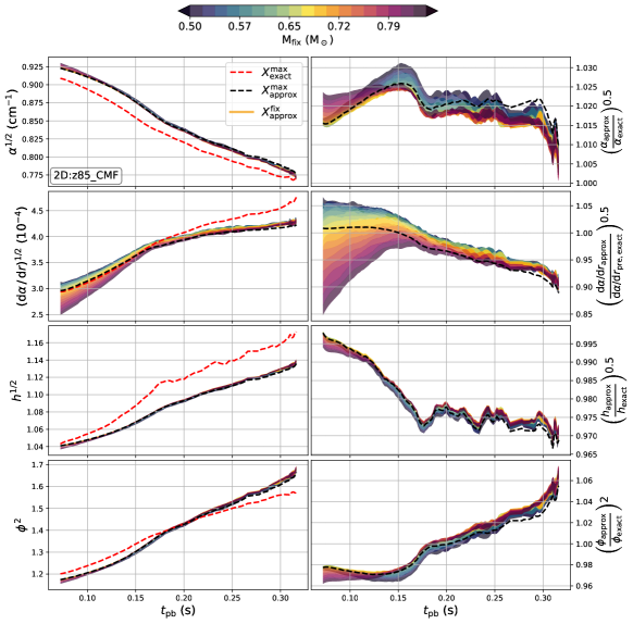
Figure 2: Left panel: Approximations for the lapse function $\alpha$, its derivative $\mathrm{d}\alpha/\mathrm{d}r$, conformal factor $\phi$, and relativistic enthalpy $h$ for the 2D model z85:CMF. Right panel: Relative errors of the respective approximations. Red dashed lines show the exact values, black dashed lines show the approximations at the maximum of the Brunt-Väisälä frequency, and coloured lines shows the mass coordinates of the fixed-mass shell approximation. The orange line ($X^{\mathrm{fix}}_{\mathrm{approx}}$) corresponds to our default choice for $M_{\mathrm{fix}}$.

To conclude, the relative error at late times in Fig. 2 is primarily caused by the term $\left(\mathrm{d}\alpha/\mathrm{d}r\right)^{1/2}$. This error, in turn, is mostly due to the choice of the mass coordinate $M_{\mathrm{mode}}$ that appears in the approximation for the derivative of the lapse function $\alpha$. Approximating the derivative analytically for any given mass coordinate introduces a smaller error. We also note that, during the signal interval, the terms appearing in the effective relativistic acceleration are only slightly sensitive to the fixed mass shell.

3.2.2 EoS and PCS structure terms

We next turn our attention to the “EoS factor” appearing in the Brunt-Väisälä frequency in Equqation (1). As a first approximation, we neglect the term $\left({\partial P}/{\partial Y_{\mathrm{e}}}\right)_{\rho,s}\mathrm{d}Y_{\mathrm{e}}/{\mathrm{d}r}$ as it is about a factor $\mathord{\sim}12$ smaller than the first term $\left({\partial P}/{\partial s}\right)_{\rho,Y_{\mathrm{e}}}{\mathrm{d}s}/{\mathrm{d}r}$ during our the time interval of interest. We define the EoS parameter $c_{\mathrm{eos}}$ as

$$c_{\mathrm{eos}}\equiv\left(\partialderivative{P}{s}\right)^{1/2}_{\rho,Y_{\mathrm{e}}}/c_{\mathrm{s}},$$ (6)

so that $\omega_{\mathrm{BV}}^{2}$ becomes,

$$\omega_{\mathrm{BV}}\approx c_{\mathrm{gr}}c_{\mathrm{eos}}\sqrt{\frac{1}{r^{2}\rho}\derivative{s}{r}}=c_{\mathrm{gr}}c_{\mathrm{eos}}\sqrt{\frac{4\pi r^{2}\rho}{r^{2}\rho}\derivative{s}{m}}=c_{\mathrm{gr}}c_{\mathrm{eos}}\sqrt{4\pi\derivative{s}{m}}.$$ (7)

The radial profiles of the angle-averaged entropy do not vary substantially for the first few hundreds of milliseconds after bounce. Furthermore, the homologous core mass at bounce and the entropy profiles at the edge of the PCS core are not strongly sensitive to progenitor variations. The sensitivity to progenitor variations may actually be overaccentuated by the use of the deleptonisation scheme of Liebendörfer (2005) as an approximation during the collapse phase. This means that we can treat the entropy gradient in Equation (7) as only (weakly) dependent on the EoS, and relatively universal across progenitors. Based on our simulations, we choose a value of $\mathrm{d}s/\mathrm{d}m\approx 11.93k_{\mathrm{B}}/\mathrm{M}_{\odot}$ for the entropy gradient.

To demonstrate our approximation for $c_{\mathrm{eos}}$, we show the factors $c_{\mathrm{s}}$ and $(\partial P/\partial s)_{\rho,Y_{\mathrm{e}}}^{1/2}$ in Equation (6) at fixed mass coordinates in Figure 3 and compare them to their actual values at the peak of the Brunt-Väisälä frequency. This is similar to our verification of the approximations for the metric terms in Figure 2. As is evident from the relative error in the right column, the best fit for the speed of sound in Panel 1 is again obtained approximately for $M_{\mathrm{fix}}\approx 0.7\,\mathrm{M}_{\odot}$, with errors of $\lesssim 10\%$. For both quantities, the error increases (see right column), reaches a maximum, and then decreases again: $M_{\mathrm{fix}}$ is initially chosen at a slightly larger mass coordinate than the core $g$-mode; as the mass coordinate of peak of the Brunt-Väisälä frequency wanders inside and closer to $M_{\mathrm{fix}}$, the error becomes smaller, and then increases again as the peak of the Brunt-Väisälä frequency moves to mass coordinates smaller than $M_{\mathrm{fix}}$. This behaviour is even better understood from Figure 4, which shows the angle-averaged sound speed and density profiles, for model z85:CMF. Vertical lines in the top panel denote the mass coordinate of the maximum Brunt-Väisälä frequency $\omega_{\mathrm{BV}}^{2,\mathrm{max}}$ as a function of time; the dashed vertical line in the second row denotes the fixed mass shell coordinate $M_{\mathrm{fix}}=0.72\,\mathrm{M}_{\odot}$. The mismatch between $M_{\mathrm{fix}}$ and $M_{\mathrm{\omega_{\mathrm{BV}}^{\mathrm{2,max}}}}$ is reflected in an underestimation of the sound speed as relevant to the $g$-mode at later times.

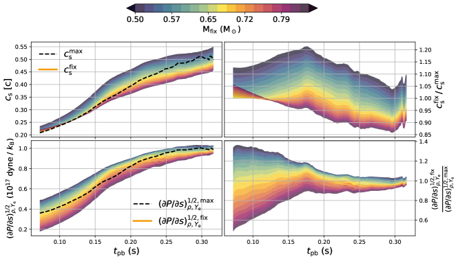
Figure 3: Top row: Angle-averaged sound speed $c_{\mathrm{s}}$ at a fixed mass mass coordinate $M_{\mathrm{fix}}$ (coloured lines with colour bar at the top) for the 2D model z85:CMF. The black dashed line shows $c_{\mathrm{s}}$ at the peak of the Brunt-Väisälä frequency. Bottom row: Same plot for the square root of the thermodynamic derivative $\left(\partial P/\partial s\right)^{1/2}_{\rho,Y_{\mathrm{e}}}$. The panels on the right show the corresponding relative errors for different mass coordinates.

We also notice that the maximum of the Brunt-Väisälä frequency is accompanied by a larger gradient $\mathrm{d}\rho/\mathrm{d}m$ (visible as more densely packed lines in the lower panel). Since the sound speed is highly sensitive to the density, $c_{\mathrm{s}}$ also exhibits a greater rate of change in this region (cp. the steepening of lines in the upper panel). The reason for the increased rate of change in density is the characteristic step in the entropy profile from shock heating shortly after bounce. The CMF models exhibit faster contraction, the trend for underestimating $c_{\mathrm{s}}^{2}$ is thus accentuated compared to z85:SFHx. This leads to an overestimation of the mode frequency at late times. The deviation is particularly evident in the spectrograms of Figure 5 (Panel 1) for z35:CMF, where the “erroneously” small sound speed (appearing in the denominator), and the fixed mass approximation (dashed black) together lead to a significant overestimation of the peak frequency.

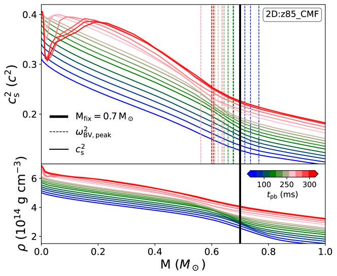
Figure 4: Angle-averaged squared sound speed (top panel) as function of mass coordinate at different time steps (see bottom right colour bar) for the 2D model z85:CMF. The coloured vertical lines indicate the maximum of $\omega_{\mathrm{BV}}^{2}$, tracked over time. The thick black line in the toppanel shows the fixed mass coordinate $M=0.72\,\mathrm{M}_{\odot}$. Angle-averaged density profiles are shown in the bottom panel. We notice that the core $g$-mode region exhibits a steeper density profile (more densely packed lines, accompanied by a steeper radial speed of sound profile).

3.2.3 Approximation for the core $g$-mode frequency

Putting together our approximations for $c_{\mathrm{gr}}$ and $c_{\mathrm{eos}}$, we obtain the analytic mode relation for the core $g$-mode,

$$\tilde{\omega}_{\mathrm{BV}}^{\mathrm{approx,fix}} =\frac{c_{\mathrm{calib}}\omega_{\mathrm{BV}}^{\mathrm{approx,fix}}}{2\pi}$$

$$\approx 0.55\times\sqrt{\frac{1}{\pi}GM_{\mathrm{mode}}\alpha_{\mathrm{approx}}^{5}\frac{1}{c_{\mathrm{s}}^{2}}\left(\partialderivative{P}{s}\right)_{\rho,Y_{\mathrm{e}}}\times 11.93\,\,k_{\mathrm{B}}/\mathrm{M}_{\odot}},$$ (8)

where we used an additional dimensionless calibration factor $c_{\mathrm{calib}}=0.55$.

We show our mode relation in the spectrograms of Figure 5. We present fits for the three 2D models of Jakobus et al. (2023), i.e., z85:CMF, z35:CMF, and z85:SFHx (from left to right). Each of the three columns shows,

1. GW spectrograms with overplotted lines for mode frequency fits.

2. the effective relativistic acceleration appearing in the Brunt-Väisälä frequency, $c_{\mathrm{gr}}~{}\equiv~{}\left[{\mathrm{d}\alpha}/{\mathrm{d}r}\!\cdot r^{2}{\alpha}/{(h\phi^{4})}\right]^{1/2}$,

3. the EoS-factor $c_{\mathrm{eos}}\equiv\left(\partial{P}/{\partial s}\right)^{1/2}_{\rho,Y_{e}}/c_{\mathrm{s}}$,

4. the radial entropy gradient $\mathrm{d}s/\mathrm{d}m$.

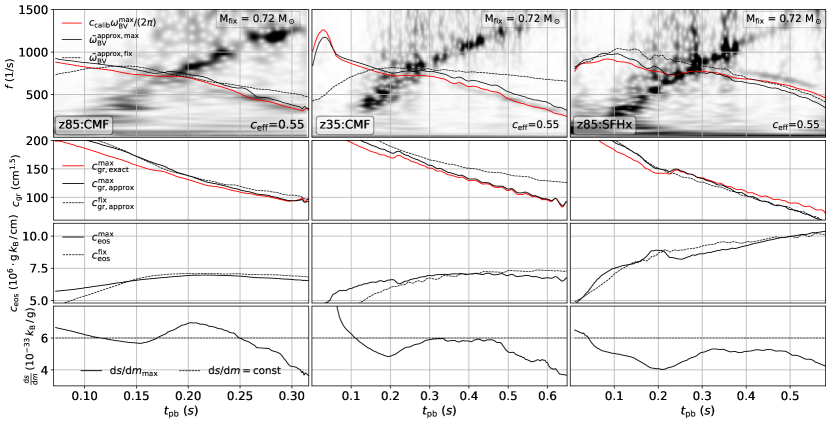
Figure 5: First row: Spectrograms with overplotted mode fits for the 2D models z85:CMF, z35:CMF, and z85:SFHx (left to right). Red lines correspond to the square root of the actual Brunt-Väisälä frequency (divided by a factor $2\pi$). Black solid lines show the approximation $\tilde{\omega_{\mathrm{BV}}}^{\mathrm{approx,max}}$ from Equation (3.2.3), but evaluated at the actual peak of the Brunt-Väisälä frequency. Black dashed lines show the frequency $\tilde{\omega}_{\mathrm{BV}}^{\mathrm{approx,fix}}$ evaluated at a fixed mass coordinate $M_{\mathrm{fix}}$, which is displayed in the upper right corner of each panel. The second row shows the prefactor $c_{\mathrm{gr}}$, comparing the actual value of the prefactor $c_{\mathrm{gr,exact}}^{\mathrm{max}}$ at the peak of the Brunt-Väisälä frequency, the analytic approximation $c_{\mathrm{gr,approx}}^{\mathrm{max}}$ evaluated at the actual maximum of $\omega_{\mathrm{BV}}^{2}$, and the analytic approximation $c_{\mathrm{pre,approx}}^{\mathrm{fix}}$ evaluated at mass coordinate $M_{\mathrm{fix}}$. The third row shows the EoS factor $c_{\mathrm{eos}}$ at both the maximum of $\omega_{\mathrm{BV}}^{2}$ in solid black ($c_{\mathrm{eos}}^{\mathrm{max}}$), and at a fixed mass coordinate $M_{\mathrm{fix}}$ ($c_{\mathrm{eos}}^{\mathrm{fix}}$). The last row compares the entropy gradient at the maximum of $\omega_{\mathrm{BV}}^{2}$ (solid curve) to our approximation of a constant entropy gradient (dashed horizontal line).

The first row shows the actual peak value $f^{\mathrm{peak}}$ of the Brunt-Väisälä frequency , multiplied by a factor $c_{\mathrm{calib}}/(2\pi)$, in red lines for all three progenitors, with the simulation spectrograms shown in the background (in black and white). We further display the approximation from Equation (3.2.3), evaluated at the actual peak of $\omega_{\mathrm{BV}}^{2}$ in black solid lines, and at a fixed mass shell in black dashed lines, with the respective fixed mass coordinate indicated in the upper right corner of each spectrogram. We chose a fixed mass coordinate of $M_{\mathrm{fix}}=0.72\,\mathrm{M}_{\odot}$ for all three progenitors and $c_{\mathrm{eff}}=0.55$ (see Eq. 3). The approximation at $\omega_{\mathrm{BW}}^{\mathrm{2,max}}$ (black lines) and the exact form of $\omega_{\mathrm{BV}}^{2}$ (red lines) align fairly well (below $\mathord{\sim}10\%$ relative error). We underestimate the mode frequency towards late times for progenitor z85:SFHx. The frequency approximation for z35:CMF is somewhat inaccurate, particularly at later times. Choosing a constant mass shell coordinate is the reason for this deviance as we will discuss below.

The second row shows the relativistic prefactor $c_{\mathrm{gr}}$ (red) and our approximation at the maximum of the Brunt-Väisälä frequency (solid black). Analogously to the top row, the dashed black line shows the approximation at a fixed mass shell $M_{\mathrm{fix}}$ (dashed black). The curves for the analytic approximations align fairly well in the $85\mathrm{M}_{\odot}$ progenitor for both EoS (CMF and SFHx), but somewhat less so for the dashed curve in the top row that relies on the assumption of a fixed mass coordinate for the buoyancy jump. By contrast, the lighter progenitor z35:CMF is clearly not well captured by the fixed mass approximation (although the fit at the maximum Brunt-Väisälä frequency aligns very well). The reason for the misalignment is the direct dependence of the frequency on the square root of the core $g$-mode mass coordinate (see $f^{\mathrm{peak}}\propto M_{\mathrm{mode}}^{0.5}$ in Eq. 3.2.3). Since the core $g$-mode mass coordinate shifts towards lower values as function of time, the mode is overestimated at later times. This behaviour is sightly evident in z85:CMF as well, albeit to lesser extent.

The third row, we show the EoS parameter $c_{\mathrm{eos}}$. We compare values extracted at the peak frequency (solid black), and the ones obtained at mass coordinate $M_{\mathrm{fix}}$. Since we want to probe the EoS parameter, there is no approximation for the latter. The parameter $c_{\mathrm{eos}}$ is strongly sensitive to the location of the fixed mass shell.

In the bottom row of Figure 5, we compare the time evolution of the entropy gradient $\mathrm{d}s/\mathrm{d}m$ at the peak of the Brunt-Väisälä frequency to our approximation of a constant value for $\mathrm{d}s/\mathrm{d}m$. Clearly, $\mathrm{d}s/\mathrm{d}m$ is overestimated at later times. The decrease of $\mathrm{d}s/\mathrm{d}m_{\mathrm{max}}$ at late times is the result of neutrino diffusion and possibly convective overshoot into the stable right. Next to the specification of a fixed mass coordinate $M_{\mathrm{fix}}$, this marks the second largest error source in our analytic mode relation.

$\alpha$	$1-Gc^{-2}\left[{M_{\mathrm{mode}}}/{r_{\mathrm{mode}}}-{(M_{\mathrm{NS}}-M_{\mathrm{mode}})}/{\langle r\rangle}\right]$
$\phi$	$\alpha^{-1/2}$
$h$	$\alpha^{-1/2}$
$\mathrm{d}\alpha/\mathrm{d}r$	$Gc^{-2}M_{\mathrm{mode}}h/(r_{\mathrm{mode}}\phi^{2})^{2}$
$\mathrm{d}s/\mathrm{d}m$	$11.93\,\,k_{\mathrm{B}}/\mathrm{M}_{\odot}$
$\left(\partial P/\partial Y_{\!\mathrm{e}}\right)_{\rho,s}\mathrm{d}Y_{\!\mathrm{e}}/\mathrm{d}r$	neglect as $\ll\left({\partial P}/{s}\right)_{\rho,Y_{\mathrm{e}}}{\mathrm{d}s}/{\mathrm{d}r}$
$\left({\partial P}/{\partial s}\right)_{\rho,Y_{\mathrm{e}}}$	EoS dependent parameter
$c_{\mathrm{s}}$	EoS dependent parameter

Table 1: Summary of approximations for the terms in the Brunt-Väisälä frequency. The last two quantities, $\left(\partial P/\partial Y_{\!\mathrm{e}}\right)_{\rho,s}\mathrm{d}Y_{\!\mathrm{e}}/\mathrm{d}r$ and $c_{\mathrm{s}}$, are EoS parameters that need to be obtained for appropriate thermodynamic conditions based on a time-dependent solution of the PCS structure.

4 Properties of the PCS convection zone

In this section, we characterise the convective properties of the PCS. In particular, we focus on factors that may affect the excitation of the core ${}^{2}\!g_{1}$ mode and explain why the GW signal from the core $g$-mode is absent in our 3D simulation. For this reason, we restrict our analysis to the $85\,\mathrm{M}_{\odot}$ progenitor with the CMF EoS and compare results for the 2D and 3D simulations.

4.1 Explosion dynamics

Before turning to PCS convection, we briefly discuss the dynamical evolution and explosion properties of the 2D and 3D models of the z85:CMF model. For this purpose, Figure 6 shows the the baryonic PCS mass $M$, the PCS radius $R$, the diagnostic explosion energy $E_{\mathrm{expl}}^{\mathrm{diag}}$, the mass accretion rate onto the PCS, and the angle-averaged shock radius $R_{\mathrm{shock}}$ for the 2D and 3D simulation.

Both the 2D and 3D model undergo shock revival. While the 2D model forms a black hole at a post-bounce time of $\mathord{\sim}330\,\mathrm{ms}$, the 3D model does not reach black hole formation before the end of the simulation at $\mathord{\sim}430\,\mathrm{ms}$. In both models, the explosion dynamics are comparable to the z85 run in Powell et al. (2021), which was, however, performed with the SFHx EoS. In the 3D simulation, the baryonic PCS mass is slightly increased, reaching $\mathord{\sim}2.55\,\mathrm{M}_{\odot}$, along with a decreased mass accretion rate. The PCS radius is predominantly determined by the PCS EoS and reaches similar final values of $\mathrm{\sim}24-25\,\mathrm{km}$, but PCS contraction is slightly faster in 2D. Note that there some early differences in the PCS mass, mass accretion rate, and shock trajectory right after bounce. We have traced these to slightly different collapse dynamics in both models. To avoid artefacts from slightly imperfect matching between the low-density EoS and the SFHx EoS at intermediate densities, the switch between those EoS regimes was set at a higher density in the 2D model during the initial collapse phase than in the 3D model. The transition density was then set to the same value before significant electron fraction and entropy changes occur later in the collapse, but this imprinted small entropy differences between 2D and 3D in parts of the core, and resulted in slightly different collapse times of $0.43\,\mathrm{s}$ in 3D and $0.49\,\mathrm{s}$ in 2D. The mass of the homologous core differs slightly between 2D ($0.7\,\mathrm{M}_{\odot}$) and 3D ($0.67\,\mathrm{M}_{\odot}$) as do the post-bounce entropy profiles, and this then also affects the dynamics of prompt convection. These differences, compounded by the stochasticity preclude a perfect comparison of the 2D and 3D model and illustrate once again a non-negligible sensitivity of the post-collapse phase to the collapse physics (cp. Lentz et al., 2012).

In the 2D simulation, shock revival occurs at $\mathord{\sim}150\,\mathrm{ms}$, whereas in the 3D simulation, it occurs slightly later at $\mathord{\sim}180\,\mathrm{ms}$. The diagnostic explosion energy, which we compute in general relativity following (Müller et al., 2012b), reaches comparable values in both cases. The explosion energy in these two CMF models is higher than that of the 3D model with the SFHx EoS computed by Powell et al. (2021).

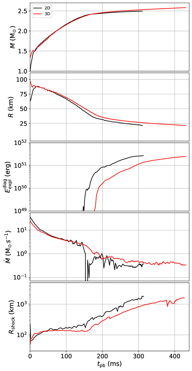
Figure 6: Time evolution of PCS mass (first row), PCS radius (second row), diagnostic explosion energy (third row), mass accretion rate (fourth row), and angle-averaged shock radius (fifth row). Both models undergo shock revival within $155-180\,\mathrm{ms}$ after core bounce. The 3D model does not reach black hole formation before the end of the simulation.

4.2 Time variability of the quadrupole moment

We observe a strong core $g$-mode signal for model 2D:z85, but not for model 3D:z85. There are three possible reasons for the less efficient excitation of the core $g$-mode by PCS convection in 3D. The turbulent kinetic energy in the convection zone may be smaller, less of the turbulent kinetic energy may be contained in quadrupole motions, and the frequency spectrum of convective motions may overlap less with the mode frequency. We first investigate the possibility of a smaller turbulent kinetic energy in the PCS convection zone in 3D. To this end, we compute the turbulent kinetic energy inside the PCS, defined as

$$E_{\mathrm{kin,turb}}^{\mathrm{PCS}}=\frac{1}{2}\int_{\mathrm{\rho\geq 10^{11}\,\mathrm{g\,cm}^{-3}}}\rho v_{\mathrm{turb}}^{2}\mathrm{d}V,$$ (9)

where $v_{\mathrm{turb}}=v_{r}^{{}^{\prime}2}+v_{\theta}^{2}+v_{\phi}^{2}$ and $\mathrm{d}V=\phi^{6}r^{2}\sin\theta\,\mathrm{d}\phi\,\mathrm{d}\theta$ in general relativity. The quantity $v_{r}^{{}^{\prime}}$ is the Favrian radial velocity perturbation, which is obtained from the Favre (i.e., density weighted) average $\langle v_{r}\rangle$ as $v_{r}^{{}^{\prime}}=v_{r}-\langle v_{r}\rangle$ . The turbulent kinetic energy as a function of post-bounce time for the 3D and 2D simulations is shown in Figure 7. In both models, the turbulent kinetic energy saturate at similar values of approximately $8\times 10^{50}\,\mathrm{erg}$. In the 3D simulation, however, the increase occurs abruptly, around $180\,\mathrm{ms}$ after bounce, compared to 2D, where the turbulent kinetic energy builds up more slowly within $\mathord{\sim}100\,\mathrm{ms}$. Hence the absence of the core $g$-mode signal in 3D cannot be ascribed to weaker convective forcing.

We therefore investigate the second potential explanation, i.e., that a lack of power in $l=2$ perturbations could explain the less efficient excitation of the core $g$-mode excitation.

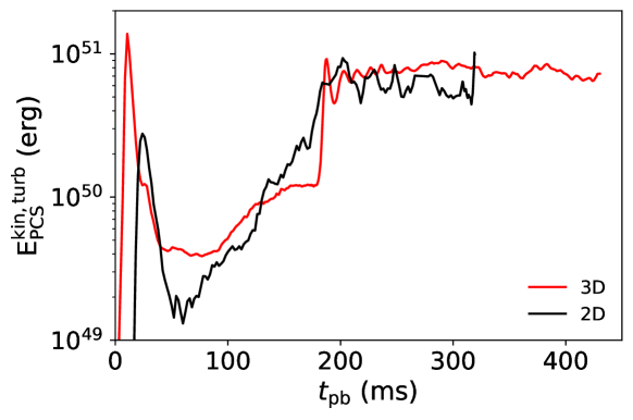
Figure 7: Time evolution of the PCS turbulent kinetic energy for 2D (black line) and 3D (red line); see Equation (9) for the definition of the turbulent kinetic energy. Both models exhibit similar turbulence strengths in the PCS. The 3D run has a sudden “step” at $\mathord{\sim}180\,\mathrm{ms}$, during which the turbulent kinetic energy rises sharply.

For this purpose, we compare the turbulent energy spectra $E(l)$ as function of the multipole order $l$ in 2D and 3D at two different post-bounce times in the first row of Figure 8. We decompose the radial turbulent convective motion into spherical harmonics $\mathcal{Y}_{\mathrm{lm}}(\phi,\theta)$ according to

$$E(l)=\frac{1}{2}\sum_{m=-l}^{l}\bigg{\rvert}\int\mathcal{Y}_{lm}^{*}v_{r}\sqrt{\rho}\,\mathrm{d}\Omega\bigg{\rvert}^{2},$$ (10)

where we sum over modes corresponding to the same multipole order $l$. In order to obtain smoother spectra, we average over five radial zones in the 3D run and 30 radial zones in the 2D run, and average over a time window of approximately $10\,\mathrm{ms}$.

In Kolmogorov’s theory of turbulence, the energy spectrum is determined by a forward energy cascade to small scale with a $E(l)\propto l^{-5/3}$ scaling law in the energy spectrum (Kolmogorov, 1941). In this case, turbulent energy is injected by external sources at the largest (spatial) scales and cascades to smaller scales. Conversely, turbulence in 2D undergoes an “inverse turbulent energy cascade” wherein turbulent energy is transferred from small scales to large scales (Kraichnan, 1967). These different behaviours significantly affect the post-shock dynamics (Murphy & Meakin, 2011; Hanke et al., 2013).

In Figure 8, we show the $5/3$ power-law as a green line, and the $l^{-3}$ power-law as dashed green. The power spectrum observed in the 3D run aligns well with the predictions of turbulent theory for length scales $l\gtrsim(15\texttt{-}40)$ where energy is transferred to small scales until dissipation becomes prominent at $l\approx 40$. In 2D, the spectrum fluctuates heavily, but is roughly consistent with an inverse cascade with a $5/3$ power-law below $l=10$. At smaller scales $l\gtrsim 15$ the 2D run roughly follows a $l^{-3}$ forward enstrophy cascade, see dashed green line (Kolmogorov, 1941; Kraichnan, 1967; Hanke et al., 2012). Based on these snapshots, it is difficult to judge, however, whether quadrupolar motions are generally stronger in 2D.

Better insights can be gained from the second panel of Figure 8, which presents the time evolution of the power $E(2)$ in quadrupole motion in the 3D run (dotted red lines) and the 2D run (dotted black lines). The turbulent quadrupole motion exhibits comparable magnitudes in the 2D and 3D simulations on average, but we observe a significantly higher level of temporal variability in the 2D run. Additionally, in the 2D run, we observe enhanced power at lower scales with $l\lesssim 10$ and a relatively smaller proportion of power at small scales, compared to the total power $E_{\mathrm{tot}}$ (solid lines, see distance of solid lines versus dashed lines). This is a consequence of the $l^{-3}$ scaling law in 2D.

Figure 8: Top panel: Turbulent energy spectrum $E(l)$ from Equation (10), evaluated at $13\,\mathrm{km}$ for the 3D run (red), and at $11\,\mathrm{km}$ for the 2D run (black) at two different times as indicated in the legend in the upper right. We choose a slightly smaller radii in 2D, as the convective zones is located further inside compared to 3D. Middle panel: Time evolution of different components of the turbulent energy spectrum (3D: red, 2D: black), i.e., the quadrupolar power $E(2)$, the power at $l\leq 10$, and the total power $E_{\mathrm{tot}}$ over the entire spectrum evaluated as well at 13 km for the 3D run, and 11 km for the 2D run. Bottom panel: Autocorrelation function of the quadrupole spectral power $E(2)$ in 3D (red shaded) and 2D (black shaded) as computed from Equation (11). The time interval for the computation of the autocorrelation function is indicated as the grey-shaded area in the middle panel. The first panel shows increased variability in the power spectrum as a function of different multipole order $l$ in 2D compared to 3D. We further observe increased time variability of the quadrupolar moment in 2D (middle panel) and a shorter autocorrelation time (bottom panel).

It should be noted here that, although $E_{\mathrm{tot}}$ is marginally higher in the 2D run, the turbulent energies $E_{\mathrm{kin,turb}}^{\mathrm{PCS}}$ in Figure 7 are of similar order.

To further quantify the time variability of PCS convection in 2D and 3D, we plot the autocorrelation function of $E(2)(t)$ in the third panel of Figure 8. The autocorrelation function $r(t)$ of a function $E(t)$ is given by

$$r(t)=\int E(t+\tau)E(\tau)\,\mathrm{d}\tau,$$ (11)

which we evaluate using a discrete time series with sampling rate $\tau=10^{-3}\,s$ for $E(2)(t)$. To avoid non-stationary trends, we use a time interval in which the quadrupolar strength is roughly constant in between $\mathord{\sim}180\texttt{-}310\,\mathrm{ms}$ for both 2D and 3D. The grey shaded areas in the second panel of Figure 8 indicate the time interval. It is evident that the autocorrelation time $\tau_{\mathrm{corr}}$ (which we define as the first zero of the correlation function) in the 2D run is notably shorter compared to the 3D run. This disparity between 3D and 2D could be attributed to factors such as faster decay rates of eddies or a greater velocity dispersion around the typical convective velocity within the turbulent flow, or simply by greater temporal variability in a 2D system in which a smaller number of modes has to carry roughly the same convective flux as in 3D.

To further assess the stronger temporal variability of quadrupolar motions in 2D as a factor for the emergence of the core $g$-mode signal, one could also consider (temporal) Fourier transforms of the turbulent energy spectrum. The Wiener-Khinchin theorem relates the Fourier transform and the autocorrelation function (Khintchine, 1934)

$$r(t)=\mathcal{F}_{f}\left(|(\tilde{E}(f)|^{2})\right)(t),$$ (12)

where $\tilde{E}(f)=1/\sqrt{2\pi}\int E(t)e^{-2\pi ift}\mathrm{d}t$ is the Fourier transform of $E(t)$ and $\mathcal{F}_{f}$ denotes the Fourier transform of the power spectral density $|(\tilde{E}(f)|^{2}$. Contrary to the Fourier transform, the autocorrelation has no phase information (due to the magnitude-squared operation), so it is not possible to invert Equation (12) to obtain the Fourier transform $\tilde{E}(f)$. The retention of phase information in the Fourier transform comes at the price of a rather noisy signal in the frequency domain compared to the rather smooth autocorrelation function, however.

Nonetheless, it is instructive to compute the temporal Fourier transforms of the turbulent energy spectrum $E(l)$ for $l\leq 10$ in the post-bounce time window $180\,\mathrm{ms}\mathord{\leq}t\mathord{\leq}310\mathrm{ms}$ (Figure 9) in 3D (upper panel), and 2D (lower panel). We note the increased power at higher frequencies in 2D, which once more reflects the stronger variability of convection on short time scales in 2D, as already pointed out in our analysis of the correlation time for the quadrupole moment.

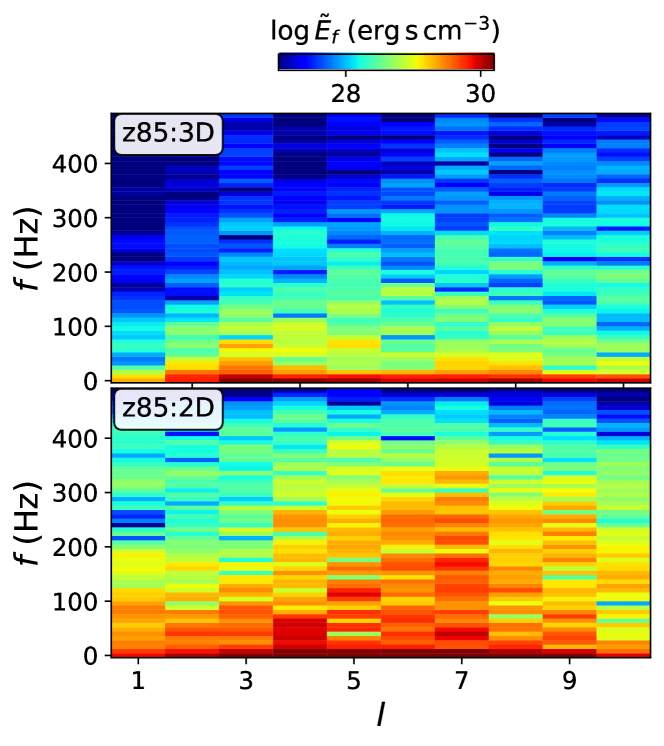
Figure 9: Temporal Fourier transform of the turbulent energy spectrum $E(l)$ for $l\leq 10$, computed for the same time interval as the autocorrelation function in Figure 8, i.e., during the window $\mathord{\sim}180\texttt{-}310\,\mathrm{ms}$. More power at high frequency is observed in the 2D run, reflecting stronger temporal variability of the convective energy in quadrupolar motions on short time scales.

To wrap this subsection up, we briefly summarize our findings: In Fig. 8, the decomposed turbulent motion in the PCS convection zone exhibits a $l^{-5/3}$ scaling law at intermediate harmonic degrees $l\gtrsim 15$ in 3D, and a steeper $l^{-3}$ decline in 2D at intermediate degrees $l\gtrsim 15$, which is both in accordance with turbulent theory (Kraichnan, 1967; Kolmogorov, 1941; Landau & Lifshitz, 1959). The inverse cascade in 2D is less established at small $l\lesssim 5$, and 2D and 3D show similar behaviours here. There is more power though at low, and intermediate harmonic degrees $5\lesssim l\lesssim 15$ in 2D, as we would expect from an inverse cascade (this is more so the case at later postbounce time $\mathord{\sim}300\,\mathrm{ms}$). The second thing we notice is a large temporal variability of the turbulent quadrupole in 2D compared to 3D (second panel of Fig. 8). This is reflected in a shorter correlation time of the time evolution of $E(2)$ (third panel), and as increased power at higher frequencies in the Fourier spectra $\tilde{E}(l)$ in Fig. 9.

We can thus summarise our analysis of the possible reasons for weaker excitation of the core $g$-mode as follows. As shown in Figures 7 and 8, the total turbulent kinetic energy and the energy in quadrupolar motions are not significantly reduced in 3D compared to 2D in a time-averaged sense. The most likely explanation for the lack of the core $g$-mode signal in 3D is therefore the increased correlation time, smaller temporal variability, and smaller power at high frequencies in convective motions in 3D. This analysis supports earlier qualitative reasoning (Andresen et al., 2017) that the eddies in the 2D simulation exert more “impulsive” forcing and that their frequency spectrum overlaps to a higher degree with the natural core $g$-mode frequency, allowing for resonant excitation of the core $g$-mode oscillation.

4.3 Energy fluxes in the PCS convection zone

As discussed in the previous section, the turbulent kinetic energy is a determining factor for the excitation of oscillation modes by PCS convection and the GW emission by these modes. For convection in the gain region, one can directly relate the convective energy flux to the power in GWs (Powell & Müller, 2019; Radice et al., 2019). A similar relation has been postulated between the neutrino luminosity and GWs from modes excited by PCS convection (Müller, 2017) by invoking a balance between the neutrino luminosity and the PCS convective energy flux. It is unclear, however, how well such balance arguments hold for PCS convection. In other context, e.g., for convection during the neutrino-cooled burning stages of massive stars, such balance arguments have been discussed extensively (e.g., Müller et al., 2016). For convection driven by thin burning shells, the dominant source term must balance convective energy transport and turbulent dissipation so that the net entropy generation rate in the convective region is roughly uniform and and a build-up of a growing unstable entropy gradient is avoided. In the context of PCS convection, one might expect a similar self-regulation of the convective flux. When the convective region in the PCS cools due to the total neutrino energy flux $F_{\mathrm{rad}}^{\nu}$, the entropy gradient will be pushed towards negative values; the magnitude of the negative gradient will depend on the neutrino flux $F_{\mathrm{rad}}^{\nu}$ at the outer boundary of the convective zone. A steeper negative entropy gradient will enhance entropy-driven convection, causing hotter material from the lower layers to be transported towards the outer boundary of the convective region, resulting in a large convective energy flux $F_{\mathrm{conv}}^{\mathrm{h}}$. This counteracts the build-up of a negative entropy gradient until balance is achieved.

Figure 10: Total neutrino energy flux $F^{\nu}_{\mathrm{rad}}$ (light grey lines) at three different times with corresponding legend in the left plot, and convective energy flux $F_{\mathrm{conv}}^{\mathrm{h}}$ (black) in 2D (left) and 3D (right). The convective energy flux in 2D is averaged over $25\,\mathrm{ms}$ between $255\,\mathrm{ms}\texttt{-}280\,\mathrm{ms}$ after bounce. In both models, the total neutrino energy flux $F^{\nu}_{\mathrm{rad}}$ exceeds the convective flux $F_{\mathrm{conv}}^{\mathrm{h}}$ towards the outer convective boundary.

But although some form of balance must still govern the quasi-steady state of PCS convection, the driving of convection involves a more complex interplay of competing lepton and entropy gradients, and the relation between the bulk energy loss (i.e., the total neutrino luminosity) and the strength of convection may be complicated. In this section we will analyse what factors determine the turbulent convective energies in the PCS convection zone, e.g., whether the convective velocities can be related to the total outgoing neutrino flux.

In our analysis we shall make repeated use of spherical Reynolds and Favere averaging. We denote volume-weighted spherical Reynolds averages as $\langle.\rangle$ or hats for single averages, and mass weighted Favre averages as tildes $\tilde{X}={\langle\rho X\rangle}/{\hat{\rho}}$ (Favre, 1965). We use single primes for fluctuating quantities from Reynold averages $X^{\prime}=X-\hat{X}$, and double primes for fluctuations from Favre averages ${X}^{\prime\prime}=X-\tilde{X}$.

To analyse the quasi-steady state of PCS convection, we plot the total neutrino energy flux $F_{\mathrm{rad}}^{\nu}$, and convective energy flux $F_{\mathrm{conv}}^{\mathrm{h}}$ both 2D and 3D in Figure 10. We define the total neutrino energy flux $F_{\mathrm{rad}}^{\nu}$ as

$$F_{\mathrm{rad}}^{\nu} =4\pi r^{2}\langle F_{\nu_{\mathrm{e}}}+F_{\overline{\nu}_{\mathrm{e}}}+4F_{\nu_{\mathrm{x}}}\rangle$$

$$=\int W\alpha\phi^{4}(F_{\nu_{\mathrm{e}}}+F_{\overline{\nu}_{\mathrm{e}}}+4F_{\nu_{\mathrm{x}}})r^{2}\mathrm{d}\Omega,$$ (13)

where $W$ is the Lorentz factor, $\alpha$ the lapse function, and $\phi$ the conformal factor, and $F_{\nu_{\mathrm{e}}}$, $F_{\bar{\nu}_{\mathrm{e}}}$, and $F_{\bar{\nu}_{\mathrm{x}}}$ are the energy flux densities of electron neutrino, electron antineutrinos, and heavy-flavour neutrinos, respectively. The convective energy flux is defined as

$${F}_{\mathrm{conv}}^{\mathrm{h}} =4\pi r^{2}\langle\rho{v}_{r}^{\prime\prime}{h}^{\prime\prime}\rangle=\int\alpha\phi^{4}\rho{v}_{r}^{\prime\prime}{h}^{\prime\prime}r^{2}\mathrm{d}\Omega.$$ (14)

Both fluxes are plotted at three different time steps, as indicated in the centre right of the left panel. The 2D convective energy flux is averaged over those three time steps since it fluctuates strongly.

Notably, we do not observe a balance ${F}_{\mathrm{conv}}^{\mathrm{h}}\approx F_{\mathrm{rad}}^{\nu}$ in Figure 10. The neutrino energy flux is, in fact, multiples times larger than the convective energy flux, particularly towards the outer PCS convection zone, i.e., from the viewpoint of energy transport PCS convection is inefficient, somewhat akin to the outer layers of stellar surface convection zones (Kippenhahn & Weigert, 1994). This means that a crude estimate of the convective velocity by dimensional analysis as $v_{\mathrm{conv}}\sim[{F}_{\mathrm{conv}}^{\mathrm{h}}/(4\pi r^{2}\rho)]^{1/3}\sim[{F}_{\mathrm{rad}}^{\mathrm{\nu}}/(4\pi r^{2}\rho)]^{1/3}$ (Müller et al., 2016; Müller, 2017) will be systematically too high. The key difference compared, e.g., to the late burning stages in massive shells that explains this behaviour is the more important role of radiative diffusion throughout the convective shell and the occurrence of cooling over a more substantial fraction of the convection zone rather than just a thin layer at the boundary. This implies that one needs to consider a more complex balance for the local entropy source and sink terms $\dot{s}_{\mathrm{conv}}$ and $\dot{s}_{\nu}$ from convective and radiative energy transport, and from convective and diffusive net lepton number transport, instead of simply equating the maximum of $\mathbf{F}_{\mathrm{turb}}$ to the neutrino flux from the PCS convection zone.

For this purpose, we consider the convective lepton number flux,

$${F}_{\mathrm{conv}}^{\mathrm{lep}} =4\pi r^{2}\langle\rho{v}^{\prime\prime}{Y}^{\prime\prime}_{\mathrm{e}}\rangle$$

$$=\int W\alpha\phi^{4}\rho{v}_{r}^{\prime\prime}{Y_{\!\mathrm{e}}}^{\prime\prime}r^{2}\mathrm{d}\Omega,$$ (15)

We further compute the diffusive net lepton number flux

$${F}^{\mathrm{lep}}_{\nu} =\int W\alpha\phi^{4}(\mathcal{F}_{\nu_{e}}-\mathcal{F}_{\overline{\nu}_{e}})r^{2}\mathrm{d}\Omega,$$ (16)

where $\mathcal{F}_{\nu_{i}}=F_{\nu_{i}}/\langle E\rangle_{\nu_{i}}$ is the electron neutrino and anti-neutrino number flux density, computed from $F_{\nu_{i}}$ and the average neutrino energy $\langle E\rangle_{\nu_{i}}$.

One expects that the local rate of change

$$\dot{s}_{\mathrm{conv}}+\dot{s}_{\nu} \approx\frac{m_{\mathrm{B}}}{4\pi k_{\mathrm{B}}\rho Tr^{2}\phi^{6}}\frac{\partial}{\partial r}\left[\alpha\phi^{4}\left(F_{\mathrm{conv}}^{\mathrm{h}}+F_{\mathrm{rad}}^{\nu}\right)\right]$$ (17)

$$+\frac{\mu_{\nu}m_{\mathrm{B}}}{4\pi k_{\mathrm{B}}\rho Tr^{2}\phi^{6}}\frac{\partial}{\partial r}\left[\alpha\phi^{4}\left(F_{\mathrm{conv}}^{\mathrm{lep}}+F_{\nu}^{\mathrm{lep}}\right)\right],$$

should be approximately constant to avoid a secular build-up of an entropy gradient.

Figure 11: Divergences of convective energy flux (grey), total neutrino energy flux (dashed grey), convective lepton flux times neutrino chemical potential (black dashed), and diffusive net lepton number flux with neutrino chemical potential (black), all as function of radius at 260 ms for the 3D model. For brevity, we omit relativistic prefactors in the legend of this plot, which however enter the expressions for the divergences, see Equation (17).

We evaluate these local entropy source and sink terms in in 3D in Figure 11, where we plot the divergences of the convective energy flux (dashed grey), total neutrino energy flux (grey line), convective lepton number flux (dashed black), and the diffusive net lepton number flux (black line). Their respective (partial) sums are shown as a thick dashed red line (sum of the divergences of lepton number fluxes) and as a dash-dotted red line (sum of the divergence of energy fluxes). The divergence of the convective energy flux is somewhat counteracting the divergence of the total neutrino energy flux; the sum of both terms is shown as a dotted red line which is approximately constant albeit slightly increasing towards the outer convective boundary. The divergences of convective lepton number flux and diffusive net lepton number flux almost cancel each other although their sum becomes slightly positive towards the outer convective boundary. Since the sum of the these two is approximately zero within the PCS convection zone (dash-dotted), it is apparent by eye that the sum of all four flux divergence terms is approximately constant, with the divergences of the energy fluxes in the two terms in Equation (17) being the dominant terms. Thus, energy transport in the PCS convection zone is well described by a secular balance condition. Unfortunately, this condition of local balance $\dot{s}_{\mathrm{conv}}+\dot{s}_{\nu}\approx\mathrm{const.}$ does not lend itself easily to a simple estimate for the typical convective velocity any more.

It is still worthwhile to consider, however, whether one could obtain reasonable convective velocities if $F_{\mathrm{conv}}^{\mathrm{h}}$ were known (e.g., from mixing-length theory or from some non-local theory of turbulence). To obtain turbulent velocities $v_{\mathrm{conv}}$ from the convective enthalpy flux, one exploits that ${v}^{\prime\prime 2}\sim{h}^{\prime\prime}$ often holds between the turbulent velocity and enthalpty perturbations, so that we can estimate the convective velocity by factorising,

$$F_{\mathrm{conv}}^{\mathrm{h}}=4\pi r^{2}\langle\rho{v}^{\prime\prime}{h}^{\prime\prime}\rangle\approx 4\pi r^{2}\rho\langle{v}^{\prime\prime 2}\rangle^{1/2}\langle{v}^{\prime\prime 2}\rangle\approx 4\pi r^{2}\rho\langle{v}^{\prime\prime 2}\rangle^{3/2}.$$ (18)

Setting $v_{\mathrm{conv}}=\langle v^{\prime\prime 2}\rangle^{1/2}$ and possibly also assuming $F_{\mathrm{conv}}\sim{F}_{\mathrm{rad}}^{\nu}$ one then obtains

$$v_{\mathrm{conv}}^{\mathrm{appr}} \approx\left(\frac{{F}^{h}_{\mathrm{conv}}}{4\pi r^{2}\rho}\right)^{1/3}\approx\left(\frac{{F}^{\nu}_{\mathrm{rad}}}{4\pi r^{2}\rho}\right)^{1/3},$$ (19)

as mentioned before. Is it only the assumption $F_{\mathrm{conv}}\sim{F}_{\mathrm{rad}}^{\nu}$ that is violated for PCS convection, or is the usual assumption $v^{\prime\prime 2}\sim h^{\prime\prime}$ about the velocity and enthalpy fluctuations also problematic? Figure 12 compares the convective velocities and the self-consistent 3D RMS velocities at 260 ms post-bounce time. The convective velocities $v_{\mathrm{conv}}^{\mathrm{appr}}$ estimated from Equation (19) are shown as dashed lines (3D: red, 2D: grey), root mean squared (RMS) velocities $v_{\mathrm{conv}}\equiv\sqrt{\langle{v_{r}^{\prime\prime}}^{2}+{v_{\theta}^{\prime\prime}}^{2}+{v_{\varphi}^{\prime\prime}}^{2}\rangle}$ are shown as solid lines. Due to the high ratio of the neutrino energy flux to the convective energy flux shown in Figure 10, $v_{\mathrm{conv}}$ is clearly overestimated by Equation  19. Figure 12 shows, however, that the assumption $F_{\mathrm{conv}}\sim{F}_{\mathrm{rad}}^{\nu}$ is no the only issue. Comparing $\tilde{h}_{\mathrm{RMS}}$ and $v_{\mathrm{conv}}^{2}$ in 2D (grey) and 3D (red), we can see that $v_{\mathrm{conv}}^{2}\ll\tilde{h}^{\prime\prime}$. The squared convective velocity fluctuations are a factor $4\texttt{-}6$ smaller compared to the RMS enthalpy fluctuations. This means that the estimated convective velocity must be corrected downward by a another factor $2\texttt{-}2.5$ if ${F}_{\mathrm{conv}}^{h}$ is known.

Figure 12: (a) Convective RMS velocities $v^{\mathrm{2D/3D}}_{\mathrm{conv}}$ in 2D (black) and 3D (red) evaluated at $260\,\mathrm{ms}$ after bounce (dashed lines) In comparison to the convective velocities $v^{\mathrm{appr}}_{\mathrm{conv}}$ estimated from Equqation (19) (solid lines). The unstable regions are shaded in red for 3D, and shaded in grey for 2D. (b) RMS enthalpy fluctuations $\tilde{h}^{\prime\prime}_{\mathrm{RMS}}$ (solid), and squared RMS velocity $v_{\mathrm{conv}}^{2}$ (dashed ) for 2D (grey), and 3D (red) at $260\,\mathrm{ms}$ after bounce. Analogously to (a), we show convective regions as a shaded background.

4.4 Lepton flux and competition of electron fraction and entropy gradients

We next consider the transport of lepton number by convection in a manner analogous to the previous section and investigate the interplay of stabilising and destabilising entropy and electron fraction gradients in quasi-steady convection, following similar lines as the previous studies of Powell & Müller (2019); Glas et al. (2019).

The first panel of Figure 14 displays the convective lepton number flux and the diffusive net lepton number flux from Equations 4.3 and 16 in 2D and 3D.

Figure 13: Favre averaged electron fraction as a function of mass coordinate in 1D (grey dashed), 2D (black), and 3D (red) at a post-bounce time of $250\,\mathrm{ms}$. The electron fraction in the 3D model is significantly larger than in 2D.

The convective lepton number flux $F_{\mathrm{conv}}^{\mathrm{lep}}$ has a positive sign, whereas the net lepton number flux is generally negative (Pons et al., 1999). In 3D, both fluxes oppose each other at the outer edge of the PCS convection zone, and the net flux of diffusing and convective lepton number is almost constant, which was also discussed in Powell & Müller (2019). Thus, simple balance of fluxes approximately holds for lepton number transport in the PCS convection zone, whereas it does not apply for energy transport. This can again be understood as a result of self-adjustment of the fluxes in quasi-steady state. A strong loss of net lepton number at the convective boundary will steepen the $Y_{\!\mathrm{e}}$ profile which increases the convective lepton number flux $F^{\mathrm{lep}}_{\mathrm{conv}}$. Conversely, if ${F}^{\nu}_{\mathrm{lep}}$ is small, the $Y_{\!\mathrm{e}}$ gradient becomes flatter, which stabilises against convection and the convective lepton flux consequently decreases. This leads to a balancing behaviour of fluxes, established through self-adjustment in the PCS convection zone, and a quasi-equilibrium of fluxes of ingoing and outgoing material is maintained so that ${F}_{\mathrm{conv}}^{\mathrm{lep}}+{F}^{\nu}_{\mathrm{lep}}\approx 0$ (note the opposite sign). The key difference to energy transport is the high optical depth for electron neutrinos and antineutrinos. This leads to a rather small net lepton flux from the outer edge of the PCS convection zone, whereas the net energy flux in the PCS convection zone is largest at its outer boundary. In this situation, the convective and diffusive lepton number flux end up balancing each other almost exactly in order to ensure roughly uniform deleptonisation throughout the convection zone.

In 2D the behaviour does not quite conform to this pattern as shown by Figure 14, but some form of balancing behaviour of both fluxes may also be visible towards the outer convective boundary, where the convective lepton number flux is about equal to the emerging lepton number flux from the convective boundary. The negative diffusive lepton number flux is due to a positive gradient in the neutrino chemical potential $\mu_{\nu}$. In 3D, we see $\mathrm{d}\mu_{\nu}/\mathrm{d}r>0$ in between $12.5\,\mathrm{km}\lesssim r\lesssim 19\,\mathrm{km}$ (see red dotted points in the top and bottom row of Figure 14).

The negative gradient of $\mu_{\nu}$ also has implications for convective stability and instability (Powell & Müller, 2019). Instability against convection in the adiabatic regime (i.e.,neglecting diffusive effects) is governed by the Ledoux criterion for $Y_{\!\mathrm{e}}$ and entropy gradients (Ledoux, 1947),

$$C_{\mathrm{Ledoux}}=\left(\partialderivative{\rho}{s}\right)_{Y_{\!\mathrm{e}},P}\derivative{s}{r}+\left(\partialderivative{\rho}{Y_{\!\mathrm{e}}}\right)_{P,s}\derivative{Y_{\!\mathrm{e}}}{r}>0.$$ (20)

The pre-factor $\left(\partial{\rho}/{\partial s}\right)_{Y_{\!\mathrm{e}},P}$ is generally negative so that a negative entropy gradient acts as destabilising. The second thermodynamic derivative $\left(\partial{\rho}/{\partial Y_{\!\mathrm{e}}}\right)_{P,s}$ can have either sign so that there is no straightforward stability criterion for the sign of $\mathrm{d}Y_{\!\mathrm{e}}/\mathrm{d}r$. Powell & Müller (2019) showed that a negative lepton number gradient $\mathrm{d}Y_{\!\mathrm{e}}/\mathrm{d}r$ acts as stabilising according to the Ledoux criterion in the presence of a positive neutrino chemical potential gradient since the Ledoux criterion can be rewritten as (see Appendix B),

$$\left(\partialderivative{\rho}{s}\right)_{Y_{\!\mathrm{e}},P}\underbrace{\derivative{s}{r}}_{\approx 0}-\rho^{2}\left(\partialderivative{\mu_{\nu}}{\rho}\right)_{s,Y_{\!\mathrm{e}}}\derivative{Y_{\!\mathrm{e}}}{r} >0,$$ (21)

where $\mathrm{d}s/\mathrm{d}r$ applies to good approximation in a well-mixed convection zone. Note, however, that the opposite is not true for a negative radial neutrino chemical potential gradient.

The interplay of stabilising and destabilising entropy and electron fraction gradients in the PCS convection zone is complex. We find that the entropy gradient remains positive at the outermost and innermost parts of the convection zone (first row of Figure 14). The positive entropy gradient characterises these regions as Schwarzschild stable, e.g., $\left({\partial\rho}/{\partial s}\right)_{Y_{\!\mathrm{e}},P}{\mathrm{d}s}/{\mathrm{d}r}\mathord{<}0$, whereas $\mathrm{d}s/\mathrm{d}r\mathord{<}0$ (acting destabilising) in between $12\,\mathrm{km}\mathord{\lesssim}R\mathord{\lesssim{19}}\,\mathrm{km}$. Going from the bottom to the top of the convection zone, we first find a region where the stabilising effect of the entropy gradient (in between $8\,\mathrm{km}\lesssim R\lesssim 12\,\mathrm{km}$) is counteracted by destabilising conditions $\left(\partial\rho/\partial Y_{\mathrm{e}}\right)_{s,P}>0$ (which holds throughout the entire convection zone) and $\mathrm{d}Y_{\!\mathrm{e}}/\mathrm{d}r\mathord{>}0$, so that the criterion for a destabilising lepton gradient applies,

$$\left(\partialderivative{\rho}{Y_{\!\mathrm{e}}}\right)_{P,s}\derivative{Y_{\!\mathrm{e}}}{r}>0.$$ (22)

There is a narrow overlap region towards the centre of the convection zone in between $12\,\mathrm{km}\lesssim r\lesssim 16\,\mathrm{km}$ where both gradients act as destabilising. A little bit further outside, the destabilising negative entropy gradient is counteracted by a negative, thus stabilising $Y_{\!\mathrm{e}}$ gradient. Towards the outermost boundary, $\mathrm{d}s/\mathrm{d}r$ becomes positive and both gradients act as stabilising.

We see a significantly higher electron fraction in 3D than in 2D. The axes for the electron fraction in 2D and 3D carry different scales. This is better visible in Fig. 13, where we plot $Y_{\!\mathrm{e}}$ as a function of mass. Compared to 2D, the electron fraction in 3D is increased by about $50\%$. This surprisingly large difference is due to the extra release of lepton number in 2D during the phase of prompt convection, which can be quite violent in 2D and magnifies the aforementioned differences in the structure of the core after bounce from slightly different collapse dynamics (Section 4.1).

We briefly summarise our observations: A negative $Y_{\!\mathrm{e}}$ gradient towards the outer convective boundary acts convectively stabilising according to Eq. 21, and Eq. 22. The positive $Y_{\!\mathrm{e}}$ gradient at the center and towards the inner convective boundary, between $7.7\,\mathrm{km}$ and $12.5\,\mathrm{km}$, is consistently acting as destabilizing since $\left(\partial\rho/\partial Y_{\!\mathrm{e}}\right)_{P,s}>0$ throughout the convective region. According to the Ledoux criterion in Eq. 22, the compositional stability of a region is, therefore, only dependent on the sign of $\mathrm{d}Y_{\!\mathrm{e}}/\mathrm{d}r$. Although a negative $Y_{\!\mathrm{e}}$ gradient will act stabilizing under a positive $\mu_{\nu}$-gradient, a positive $Y_{\!\mathrm{e}}$ gradient can be destabilizing under both a positive and negative gradient $\mathrm{d}\mu_{\nu}/\mathrm{d}r$, as we see in the region $8\,\mathrm{km}\lesssim R\lesssim 16\,\mathrm{km}$. In both 2D and 3D, the majority of the convective region is unstable to entropy-driven convection, as $\mathrm{d}s/\mathrm{d}r<0$, which is counteracted by the negative, stabilizing $Y_{\!\mathrm{e}}$ gradient. We find a significantly increased electron fraction within the PCS convection zone in 3D, compared to 2D.

Figure 14: Radial profiles for z85:CMF in 2D (left column) and 3D (right) at a post-bounce time of 260 ms. Row 1: Convective lepton number flux $F_{\mathrm{conv}}^{\mathrm{lep}}$ (black), diffusive net lepton number flux $F_{\nu}^{\mathrm{lep}}$ (grey), and the sum of convective lepton number flux and diffusive net lepton number flux $F_{\mathrm{conv}}^{\mathrm{lep}}+F_{\mathrm{\nu}}^{\mathrm{lep}}$ (red). In 2D, dashed lines show averages over $\mathord{\sim}12\,\mathrm{ms}$ and the light red and grey curves represent different time steps around $260\,\mathrm{ms}$ within a window $\mathord{\sim}12\,\mathrm{ms}$. Row 2: Favre averaged entropy per baryon $\tilde{s}$ (black) and electron fraction $\tilde{Y_{\!\mathrm{e}}}$ (red, shown with an offset in 3D). Thin lines represent multiple timesteps of $\pm 2\,\mathrm{ms}$ around 260 ms. We also show the $Y_{\!\mathrm{e}}$ and $s$-profiles of a spherically symmetric simulation, denoted by 1D (dashed lines). Row 3: RMS averages of radial velocity fluctuation $\tilde{v}_{r}^{\mathrm{RMS}}$ (black) and non-radial (grey) velocites evaluated as $\tilde{v}_{\theta,\phi}=\langle\sqrt{v_{\theta}^{2}+v_{\phi}^{2}}\rangle$ Row 4: Favre averaged neutrino chemical potential (black). Grey-shaded areas represent the regions of convective instability according to the Ledoux criterion. Red dots on lines in rows 1, 2 and 5 indicate the region where the neutrino chemical potential has a positive gradient.

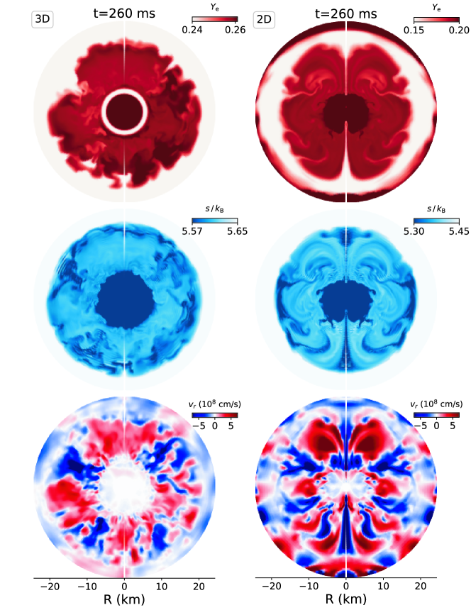
Figure 15: Slices along meridional plane showing the electron fraction $Y_{\!\mathrm{e}}$ (first row), entropy per baryon $s$ (second row), and radial velocity $v_{r}$ (third row) for 3D (left column), and 2D (right column). The PCS convection zone stretches from approximately 20 km to 8 km (visible as enhanced radial velocities in the third panel). The electron fraction in the 3D run shows a small asymmetry on the lower right side (higher $Y_{\!\mathrm{e}}$). In 2D, and to lesser extent in 3D, we see Ledoux convection, as low entropy and $Y_{\!\mathrm{e}}$ material sinks inwards. The structure in 2D is more distributed towards large scales, as expected from an inverse cascade.

4.5 Comparison to Mixing Length Theory

In order to systematically explore the dependence of the neutrino signal (Roberts et al., 2012; Mirizzi et al., 2016) and the frequency trajectory of PCS oscillations modes (Wolfe et al., 2023), e.g., on the nuclear EoS or progenitor mass and metallicity at manageable computational cost, 1D simulations remain indispensable. Especially for predicting synthetic mode frequency trajectories, it is critical that the modification of PCS stratification by multi-dimensional effects is taken into account. For this purpose, one can resort to mixing-length theory (MLT, as implemented, e.g., in Roberts et al., 2012; Mirizzi et al., 2016) or generalisations thereof (Müller, 2019b). In MLT, turbulent processes are modelled as a diffusive process, and the convective flux is carried by one-scale eddies whose dimension is of the order of the local pressure scale height (introduced below) (Prandtl, 1952; Böhm-Vitense, 1958; Weiss et al., 2004). It is useful to check how well the assumptions inherent in MLT hold in the PCS convection zone and to what extent MLT can reproduce the stratification of 3D models. For this purpose, we have conducted a 1D simulation of model z85:CMF with the mixing-length module in CoCoNuT-FMT, and we also compare turbulent fluxes and fluctuations from a Favre decomposition of the 3D model to MLT theory.

Before such a comparison, it is useful to review some basic ingredients of MLT. The turbulent diffusivity in MLT is given by $\Lambda_{\mathrm{mix}}{v}^{\prime\prime}_{\mathrm{mix}}$. The mixing length parameter $\Lambda_{\mathrm{mix}}$ is typically set as a fixed multiple of the pressure scale height,

$$\Lambda_{\mathrm{mix}}=-\tilde{P}\left(\derivative{\tilde{P}}{r}\right)^{-1}=\frac{\tilde{\rho}\,g}{\tilde{P}},$$ (23)

where Favre averages (denoted by tildes) or Reynolds averages (denoted by hats or $\langle.\rangle$) need to be used in case “virtual” MLT fluxes are to be evaluated for a 3D model. The MLT convective velocity is given in terms of $\Lambda_{\mathrm{mix}}$, the Brunt-Väisälä frequency from Equation (1), and a dimensionless parameter $\alpha_{1}$ as $v_{\mathrm{conv}}=\alpha_{1}\Lambda_{\mathrm{mix}}\omega_{\mathrm{BV}}.$ The MLT lepton number flux is then computed as

$$\langle\rho{v}^{\prime\prime}{Y_{\!\mathrm{e}}}^{\prime\prime}\rangle \approx\alpha_{1}\alpha_{2}\hat{\rho}v_{\mathrm{conv}}\Lambda_{\mathrm{mix}}\derivative{\tilde{Y_{\!\mathrm{e}}}}{r}=\alpha_{1}\alpha_{2}\hat{\rho}\omega_{\mathrm{BV}}^{2}\Lambda_{\mathrm{mix}}^{2}\derivative{\tilde{Y_{\!\mathrm{e}}}}{r},$$ (24)

where $\alpha_{2}$ is a second dimensionless coefficient. The convective energy flux in MLT is given by

$$\langle\rho{v}^{\prime\prime}{h}^{\prime\prime}\rangle \approx-\alpha_{1}\alpha_{3}\hat{\rho}v_{\mathrm{conv}}\Lambda_{\mathrm{mix}}\left(\derivative{\tilde{\epsilon}}{r}+\tilde{P}\derivative{\hat{\rho}^{-1}}{r}\right)$$

$$=-\alpha_{1}\alpha_{3}\hat{\rho}\omega_{\mathrm{BV}}\Lambda_{\mathrm{mix}}^{2}\left(\derivative{\tilde{\epsilon}}{r}+\tilde{P}\derivative{\hat{\rho}^{-1}}{r}\right),$$ (25)

Consistency with the second law of thermodynamics requires $\alpha_{2}=\alpha_{3}$ (Müller, 2019b). In our analysis, we set all the dimensionless coefficients to one, $\alpha_{1}=\alpha_{2}=\alpha_{3}=1$.

In Figure 16 we compare the MLT approximations to the actual convective lepton flux $F_{\mathrm{conv}}^{\mathrm{lep}}$ and the convective energy flux $F_{\mathrm{conv}}^{\mathrm{h}}$ from the 2D and 3D simulation. In addition, we test the approximation of optimal (linear) correlation between the turbulent fluctuations that is implicit in MLT, i.e., the approximation that the Pearson coefficient of i) radial velocity and electron fraction fluctuation and ii) radial velocity and enthalpy fluctuations equals $\pm 1$. To this end, we show factorised lepton and energy fluxes, $4\pi\langle\rho\rangle v^{\prime\prime}_{\mathrm{RMS}}{Y_{\mathrm{e}}^{\prime\prime}}_{\mathrm{RMS}}$ and $4\pi\langle\rho\rangle v^{\prime\prime}_{\mathrm{RMS}}{h^{\prime\prime}}_{\mathrm{RMS}}$ (where $X^{\prime\prime}_{\mathrm{RMS}}$ denotes RMS fluctuations of any quantity). This allows us to to better recognise whether MLT is limited i) by the approximation of fluctuations via local gradients, or ii) by the assumption of correlations between the radial velocity and thermodynamic variables.

Figure 16: Top row: Convective lepton flux $F_{\mathrm{conv}}^{\mathrm{lep}}$ (black), MLT gradient approximation (green) and factorised lepton flux (grey) for the 2D (left) and 3D (right) run. Bottom row: Convective energy flux $F_{\mathrm{conv}}^{\mathrm{h}}$, MLT gradient approximation (orange) and factorised energy flux (grey). The convective energy flux and MLT approximation for the energy flux in 2D are time-averaged over $15\,\mathrm{ms}$. For discussion, see Section 4.5.

Positive and negative fluxes correspond to upward and downward convective lepton number flows. Typically, $Y_{\!\mathrm{e}}$ is higher within the PCS core, so when high $Y_{\!\mathrm{e}}$ material is convectively transported outwards into regions with lower $Y_{\!\mathrm{e}}$, the flux $\langle\rho{v}^{\prime\prime}{Y_{\!\mathrm{e}}}^{\prime\prime}\rangle$ will be positive. Likewise, low $Y_{\!\mathrm{e}}$ material that is being transported inwards will result in a positive (outward) flux of lepton number. Both 2D and 3D simulations show a similar profile of the turbulent lepton number flux across the PCS convection zone, although the profile is less smooth in 2D. The factorised flux $4\pi\langle\rho\rangle v^{\prime\prime}_{\mathrm{RMS}}{Y_{\mathrm{e}}^{\prime\prime}}_{\mathrm{RMS}}$ tracks the actual convective lepton number flux in 3D relatively well in the outer part of the convection zone, but overestimates the actual flux considerably near the inner boundary. This indicates less correlated velocity and and electron fraction perturbations near the inner convective boundary. The MLT gradient approximation roughly captures the maximum convective lepton number flux, but even has the wrong sign in the inner part of the convection zone. The comparison of the actual convective lepton number flux is of less relevance in the artificial case of 2D axisymmetry, but is still included in the plots for the sake of completeness.

The reason why the (gradient-based) MLT approximation is generally not very accurate and becomes increasingly worse towards the inner convective boundary is better understood from Figure 17. Displayed are radial profiles of $Y_{\!\mathrm{e}}$ for different angles (latitude and longitude). The Favre average $\tilde{Y_{\!\mathrm{e}}}$ is overlayed as a blue line, together with black lines indicating the gradients $\partial\tilde{Y_{\!\mathrm{e}}}/\partial r$ at three positions (black dot); in the middle and at the outer and inner boundary of the PCS convection zone. The radial projections of the black lines show the mixing length $|\pm\Lambda|$. Comparing the vertical extent of the gradients and the dispersion of the red curves shows how well the actual $Y_{\!\mathrm{e}}$-contrast in rising and sinking plumes is captured by the extrapolated gradient across one pressure scale height. In regions where the angle-averaged profile is flat, such as in the centre of the convective boundary, the dispersion of $Y_{\!\mathrm{e}}$ is not well captured by the gradient approximation of MLT. The figure also reveals why MLT underestimates the actual convective lepton number flux and sometimes even predicts the wrong sign for the flux. The gradient of $\tilde{Y_{\!\mathrm{e}}}$ becomes positive, but is relatively small in the middle of the convection zone. Hence MLT predicts small dispersion of $Y_{\!\mathrm{e}}$, and excess $Y_{\!\mathrm{e}}$ in downdrafts and a $Y_{\!\mathrm{e}}$ deficit in updrafts. In reality, large eddies that travel beyond the mixing length transport material with very high or low $Y_{\!\mathrm{e}}$ into regions characterised by a flat local $Y_{\!\mathrm{e}}$ gradient. As a result, there can be a significant dispersion of material from relatively large rising and sinking plumes, despite a flat angular averaged radial profile. Moreover, turnover motion over the entire convection zone will transport low-$Y_{\!\mathrm{e}}$ material from the outer boundary downward and high-$Y_{\!\mathrm{e}}$ material outwards, so that the correlation of velocity and $Y_{\!\mathrm{e}}$ fluctuations has a different sign than expected from the local gradient. To capture these features, one may require a non-local theory of turbulence that better tracks the evolution of $Y_{\!\mathrm{e}}$ along the pathlines of convective flow, appropriately averaged over eddies of different scales.

The significant overestimation of the actual lepton flux by the factorised flux $4\pi\langle\rho\rangle v^{\prime\prime}_{\mathrm{RMS}}{Y_{\mathrm{e}}^{\prime\prime}}_{\mathrm{RMS}}$ near the lower boundary can also be related to the actual spatial structure of the convective flow. When large eddies fragment into small-scale turbulent motions upon reaching the convective boundary, the flow becomes dominated by random motions on small scales, so that ${v}^{\prime\prime}$ and ${Y_{\!\mathrm{e}}}^{\prime\prime}$ will become essentially uncorrelated.

In the second panel of Figure 16, we show convective energy fluxes for 2D (left) and 3D (right). The pattern is similar to what we observed for the lepton flux. The actual convective flux in 3D shows quite good agreement with the factored flux $4\pi\langle\rho\rangle v^{\prime\prime}_{\mathrm{RMS}}{h^{\prime\prime}}_{\mathrm{RMS}}$ near the outer convective boundary and in the middle of the convection zone (indicating good correlation of velocity and enthalpy in updrafts and downdrafts) but deviates from the factored flux towards the inner convective boundary. Similarly to the convective lepton flux in the upper panel, the gradient approximation $h^{\prime\prime}=\Lambda_{\mathrm{mix}}\mathrm{d}\tilde{h}/\mathrm{d}r$ gives the wrong sign for the MLT flux in parts of the convection zone around $\mathord{\sim}11\,\mathrm{km}$, although the MLT approximation appears to match somewhat better for energy transport than for lepton transport.

Despite the systematic errors in the MLT flux, the effect on the electron fraction and entropy profiles in dynamical simulation is limited. Comparing profiles from the 3D simulation and a 1D simulation with MLT in Figures 13 and 14, we find that MLT captures the average level of entropy and $Y_{\!\mathrm{e}}$ in the PCS convection zone very well. The 1D MLT model ends up with consistently negative entropy and $Y_{\!\mathrm{e}}$ gradients in the convection zone, however. The variation of these quantities within the relatively well-mixed interior of the convection zone is bigger, although the profiles still remain quite flat. Such small deviations may not compromise accuracy very much in simulations of neutron star cooling, but they may be more relevant when computing GW eigenfrequencies based on 1D profiles, and accurate profiles of the Brunt-Väisälä frequency are required.

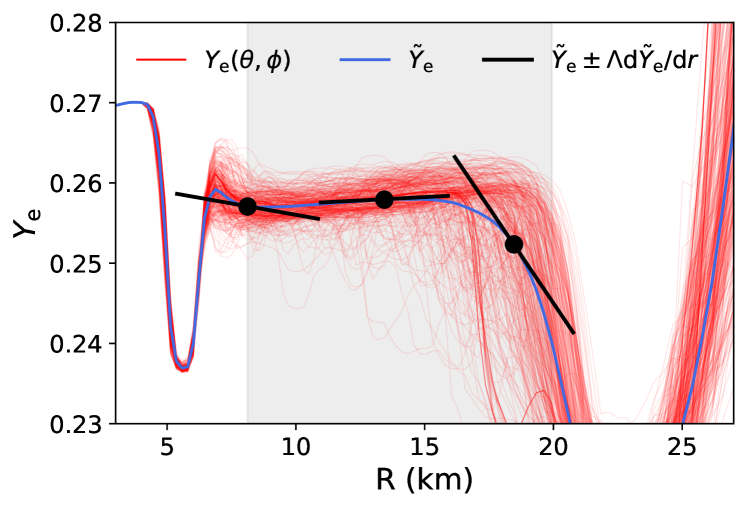
Figure 17: Radial profiles of the electron fraction $Y_{\!\mathrm{e}}$ along different angular rays (red) and Favre averaged electron fraction $\tilde{Y_{\!\mathrm{e}}}$ (blue). The gradient of $\tilde{Y_{\!\mathrm{e}}}$ is drawn (black lines) for a mixing length “step” $\pm\Lambda\mathrm{d}\tilde{Y_{\!\mathrm{e}}}/\mathrm{d}r$ at three distinct radial positions (black dots) in the PCS convection zone (grey-shaded region). The slopes of the lines show the radial gradient; their extent in the radial direction is $\Lambda(r_{i})$, evaluated as one pressure scale height, and their vertical extent gives the MLT density contrast. In the middle of the PCS convection zone, the flat gradient does not capture the dispersion of $Y_{\!\mathrm{e}}$ in rising and sinking bubbles; note in particular the region between $10\,\mathrm{km}\leq r\leq 15\,\mathrm{km}$.

4.6 Spatial structure of PCS convection

How could MLT be improved to better reproduce the correct convective energy and lepton number fluxes? For stellar convection, more general theories of convection have been proposed to incorporate non-local estimates of the contrast in advected quantities and the existence of eddies of different scales (e.g., full-spectrum turbulence; Canuto & Mazzitelli, 1992; Canuto et al., 1996). In the most abstract terms, one might compute the contrast $\delta Y_{\!\mathrm{e}}\equiv Y_{\!\mathrm{e}}(r+\Lambda)-Y_{\!\mathrm{e}}(r-\Lambda)$ (or other fluctuations) non-locally instead of applying a first-order Taylor series, and average over a range of mixing lengths $\Lambda$ with some appropriate turbulence spectrum, perhaps after taking into account effects of the turbulent cascade and non-ideal effects on eddies of various sizes. This is far beyond the scope of this paper, but the concept of non-local mixing is a good starting point for analysing the spatial structure of PCS convection and revisit the electron fraction asymmetry in the PCS that is characteristic of the LESA phenomenon (lepton-number emission self-sustained asymmetry, Tamborra et al., 2014) seen in many supernova simulations (e.g., Powell & Müller, 2019; Glas et al., 2019).

To illustrate the multi-dimensional structure of the convective flow, we show 2D slices of the electron fraction $Y_{\!\mathrm{e}}$ (first row), the entropy per baryon $s$ (second row), and the radial velocity $v_{r}$ (third row) for the 2D and 3D run at $260\,\mathrm{ms}$ after bounce in Figure 15 . In 3D and 2D, Ledoux convection pushes low entropy material with lower $Y_{\!\mathrm{e}}$ inwards, e.g., in the upper left (“11 o’clock”) of each panel both in 2D and 3D. In 3D, the patterns show more small-scale turbulence, as due to the forward turbulent cascade (Kolmogorov, 1941). High-$Y_{\!\mathrm{e}}$ material is asymmetrically “bulked” towards the lower right of the 3D run, indicative of a large-scale LESA asymmetry. In the 3D entropy plots, one can also see more clearly some sinking low-entropy plumes of smaller scale, e.g, a low entropy plume sinking inwards, e.g., at the 7 o’clock” and 10 o’clock positions. Especially the plume at 10 o’clock is also visible as a high $Y_{\!\mathrm{e}}$ plume. Large-scale structure in radial velocity are also present in 3D as in Glas et al. (2019), but the small-scale structures in velocity appear more porminent than in entropy and electron fraction. In 2D, the electron fraction, entropy, and radial velocity fields are all dominanted by large-scale structures as a manifestation of the inverse turbulent cascade in 2D (Kraichnan, 1967).

As expected, radial velocities in 2D are somewhat increased, and of larger scale, compared to 3D (Kraichnan, 1967).

To qualitatively understand the scale-dependent turbulent motions, we decompose the square roots of the radial Reynolds stress component $\rho v_{r}^{2}$, electron fraction $Y_{\!\mathrm{e}}$, and entropy $s$ per baryon into spherical harmonics (Figure 18). Spectra $\hat{X}_{l}$ of any quantity $X$ are calculated as,

$$\hat{X}_{l}=\sum_{m=-l}^{l}\left|\int\mathrm{d}\Omega\mathcal{Y}_{lm}^{*}(\theta,\phi)\sqrt{X}\right|^{2}.$$ (26)

Taking the square root of these quantities ensures that the power in the decomposition of $\sqrt{\rho}v_{r}$ can be interpreted as a kinetic energy spectrum. We normalise the spectrum $\hat{X}_{l}$ by monopole $\hat{X}_{0}$. The procedure is similar to the decomposition of the turbulent kinetic energy in Equation (10) (identical for the kinetic energy without a factor 0.5 in front of the sum).

For the velocity spectrum, we observe a Kolmogorov scaling law with a $5/3$-slope in the inertial range towards intermediate scales at angular wavenumbers above $l\gtrsim 12$. We observe a flatter scaling law at lower polynomial degrees $l\lesssim 10$, with eventually decreasing power at low wavenumbers $l\lesssim 10$. Powell & Müller (2019) already noticed the deviation from the Kolmogorov slope at lower wavenumbers and suggested that this may be related to less efficient driving of low-order modes due to the stabilising influence of the $Y_{\!\mathrm{e}}$-gradient in parts of the PCS convection zone, but it is difficult to test this hypothesis numerically. The entropy may exhibit a spectrum of similar shape as $Y_{\!\mathrm{e}}$, but there is too much noise in the entropy spectrum already at low wavenumbers to diagnose this confidently.

The scaling looks different for the electron fraction $Y_{\!\mathrm{e}}$, which was also noted by Powell & Müller (2019) as a yet unexplained feature. At low-intermediate wavenumbers $3\lesssim l\lesssim 13$, the power spectrum approximately follows a $l^{-1}$ scaling law. As pointed out by Powell & Müller (2019), this disparity is essentially LESA in the PCS, merely viewed in spectral space instead of real space. It reflects the presence of significant large-scale patterns in $Y_{\!\mathrm{e}}$ despite slow overturn on large scales and relatively more power on medium scales in the velocity field.

We propose that the different slope of the spectrum of $Y_{\!\mathrm{e}}$ is related to the fact that the electron fraction is an advected scalar quantity (similar to a passive scalar, but slightly different because the electron fraction also influences buoyancy). Passive scalars typically follow a different scaling law in turbulent flows (Batchelor, 1959; Shraiman, 2000). The distinct scaling arises from anomalous mixing (instead of the improbable event of an atypical path with typical mixing), specifically low probability configurations in which a fluid parcel travels from a large distance to the point of mixing, without much mixing and dissipation along the way (Shraiman & Siggia, 1994).

This notion can be adapted to PCS convection and linked to the discussion about the limitations of MLT as a single-scale theory of convection. If we retain the MLT notion that the $Y_{\!\mathrm{e}}$ contrast depends on the “point of origin” of material at a distance $\pm\Lambda$,

$$\delta Y_{\!\mathrm{e}}\equiv Y_{\!\mathrm{e}}(r+\Lambda)-Y_{\!\mathrm{e}}(r-\Lambda),$$ (27)

but treat $\Lambda$ as variable, representing the eddy scale, then one can motivate a Batchelor-type scaling law $\hat{Y}_{\mathrm{e}}\propto l^{-1}$. As the angular wavenumber $l$ corresponds to the number of eddies that can be fit on a meridian between $\theta=0$ and $\theta=\pi$, the eddy scale is just $\Lambda=\pi R_{\mathrm{conv}}/l$ (Foglizzo et al., 2006), where $R_{\mathrm{conv}}$ is the radius of the convective region (which we omit in the following as this is a “constant” parameter). Then Taylor expansion of $\delta Y_{\!\mathrm{e}}\sim Y_{\!\mathrm{e}}(r+\Lambda)-Y_{\!\mathrm{e}}(r-\Lambda)$ immediately yields,

$$\delta Y_{\mathrm{e}}\propto Y_{\!\mathrm{e}}(r+\Lambda)-Y_{\!\mathrm{e}}(r-\Lambda)\propto l^{-1}\frac{\partial\tilde{Y}_{e}}{\partial r}.$$ (28)

One should note the Equation (28) is expected to break down for low $l$ because the gradient approximation is no longer appropriate and because the conversion from spatial scale to angular wavenumber becomes non-trivial (see the discussion on spherical Fourier-Bessel decomposition in Fernández et al. 2014).

One can further rationalise this somewhat unintuitive scaling behaviour if we consider a balance of forcing and dissipation terms that create an destroy $Y_{\!\mathrm{e}}$-fluctuations $\delta Y_{\!\mathrm{e}}(\Lambda)$ of a single-wavenumber mode on scale $\Lambda=\pi R_{\mathrm{conv}}l$, namely generation from a background gradient $\partial Y_{\!\mathrm{e}}/\partial r$ by velocity fluctuations and damping by turbulent dissipation with a dissipation time $\tau_{\mathrm{diss}}$ set by turbulent diffusivity on scale $D=\delta v_{r}(\Lambda)\Lambda$,

$$\delta\dot{Y}_{\mathrm{e}}(\Lambda)\approx\delta v_{r}(\Lambda)\frac{\partial Y_{\!\mathrm{e}}}{\partial r}-\frac{\dot{Y}_{\mathrm{e}}}{\tau_{\mathrm{diss}}(\Lambda)}\approx v_{r}(\Lambda)\frac{\partial Y_{\!\mathrm{e}}}{\partial r}-\dot{Y}_{\mathrm{e}}\frac{\Lambda^{2}}{\delta v_{r}(\Lambda)\Lambda}.$$ (29)

This leads to $\delta Y_{\!\mathrm{e}}(\Lambda)\propto\Lambda\propto\pi/l$ in steady state, and suggests an $l^{-1}$ power spectrum. Equation (29) neglects the cascade or “transfer” terms that would appear in a full spectral turbulence model (e.g., Canuto et al., 1996) and replaces them with a simple, scale-dependent eddy viscosity. Specifically, the transfer of power from $l^{\prime}<l$ perturbations in $Y_{\!\mathrm{e}}$ to wavenumber $l$ is neglected as a generation term for fluctuations. Neglecting this contribution in favour of “local” generation of $Y_{\!\mathrm{e}}$ fluctuations at wavenumber $l$ can be justified by noting that compared to normal Kolmogorov turbulence, there is less power in velocity perturbations at small wavenumber $l$ to drive this transfer. The key idea here is that since the velocity fluctuations on scale $\Lambda$ regulate both the driving and the damping of $Y_{\!\mathrm{e}}$ fluctuations on this scale, the spectrum of $Y_{\!\mathrm{e}}$ fluctuations may be largely independent of the velocity spectrum. By such a mechanism, stronger $Y_{\!\mathrm{e}}$ fluctuations at larger scales (smaller $l$) may emerge even if the velocity spectrum does not have appreciable power at low $l$.

Undoubtedly, much further analysis will be needed to analyse the driving, damping and transfer of power int the fluctuation spectra and possibly explain the peculiar spectral properties of PCS convection rigorously form turbulence theory. Nonetheless, we believe it is useful to outline a possible mechanism for explaining the distinct spectra of $Y_{\mathrm{e}}$ and radial velocity and hence for LESA.

Figure 18: Power spectra for $\rho v_{r}^{2}$, electron fraction $Y_{\!\mathrm{e}}$ (second row), and entropy per baryon $s$ (third row), computed according to Equation (26) in 3D (left), and 2D (right). The spectra are evaluated at $13\,\mathrm{km}$ for the 3D run, and at $11\,\mathrm{km}$ for the 2D run averaged over the time interval $225\,\mathrm{ms}\leq t\leq 260\,\mathrm{ms}$ in both cases. All values have been normalised to the monopole $\hat{X}_{0}$. The radial velocity and electron fraction follow different scaling laws. The scaling law of the radial velocity follows a typical $5/3$ slope, whereas the electron fraction approximately follows a $l^{-1}$ slope. The power spectrum for the entropy is very noisy at large spherical harmonics degrees due to low-level odd-even patterns in the numerical solution.

5 Conclusions

We studied the dynamics of proto-compact star (PCS) convection and its impact on gravitational emission from general-relativistic core-collapse supernovae in 2D and 3D simulations.

In particular, we investigated the gravitational wave signal from the ${}^{2}\!g_{1}$ mode in the PCS core, which has recently been identified as a potential probe of high-density equation-of-state physics in the 2D simulations of Jakobus et al. (2023), and has also been seen in recent 3D simulations of Vartanyan et al. (2023).

Although GW emission from this mode is not expected to be universally present in core-collapse supernovae, it is useful to relate its frequency to interpretable PCS parameters. Even when the signal from the core $g$-mode is not present, such a fit could also be used to describe the emission gap that is often seen in predicted supernova GW spectrograms at the avoided crossing of the ${}^{2}\!g_{1}$ and the dominant, rising $f/g$-mode emission band. To this end, we showed that the frequency of the ${}^{2}\!g_{1}$ mode closely tracks the peak value of the Brunt-Väisälä frequency at the edge of the PCS core. We further developed a fit formula to approximate the frequency in terms of the mass and radius of the low-entropy PCS core, the neutron star mass, the entropy gradient between the PCS core and mantle, and thermodynamic derivatives at the edge of the core. Among these quantities, the core mass and the entropy gradient are relatively universal during the early post-bounce phase. Our fit formula is given by

$$\omega_{\mathrm{BV}}^{2}=c_{\mathrm{gr}}c_{\mathrm{eos}}\sqrt{4\pi\derivative{s}{m}}.$$ (30)

with the prefactors

$$c_{\mathrm{gr}} =\left[\mathrm{d}\alpha/\mathrm{d}r\cdot r^{2}\alpha/(h\phi^{4})\right]^{1/2}\,\,\,\mathrm{and}$$ (31)

$$c_{\mathrm{eos}} =\left(\partial P/\partial s\right)_{\rho,Y_{\!\mathrm{e}}}^{1/2}/c_{\mathrm{s}}$$ (32)

We tested our fit formula on 2D models for two simulations (z35:CMF and z85:CMF) using $35M_{\odot}$ and $85M_{\odot}$ progenitors with the CMF EoS (Motornenko et al., 2020) and a $85M_{\odot}$ progenitor using the SFHx EoS (Steiner et al., 2013) (the GW signal was absent in the SFHx EoS setup for the $35M_{\odot}$ progenitor). Using the Brunt-Väisälä frequency (multiplied by a calibration factor $c_{\mathrm{calib}}=0.55$) to track the mode frequency produces good results. However, given our choice for the calibration factor, the Brunt-Väisälä frequency underestimates the SFHx core $g$-mode frequency at later times. The fit formula, using our approximations for the terms arising in the Brunt-Väisälä frequency, tracks the actual mode frequently reasonably well early on, but distinctly overestimates the mode frequency for z35:CMF at later times.

Errors in the fit stem from different sources, and the most notable among them are related to the assumption of a fixed mass coordinate for the core-mantle interface:

1. The largest error source is the mass term $M_{\mathrm{mode}}$ in Equation (3.2.3) that stems from the term $\mathrm{d}\alpha/\mathrm{d}r$ in the Brunt-Väisälä frequency . Interestingly, we can approximate the term $\mathrm{d}\alpha/\mathrm{d}r$ fairly well by a simple fit although it contains the troublesome mass coordinate term $M_{\mathrm{mode}}$. The reason is that $\mathrm{d}\alpha/\mathrm{d}r$ contains the surface gravity $M_{\mathrm{mode}}/r_{\mathrm{mode}}^{2}$ which is less sensitive to the location of the mode. In the final fit formula for the mode frequency, the factor $r_{\mathrm{mode}}^{-2}$ is cancelled by another term, and the bigger error of $M_{\mathrm{mode}}$ degrades the overall fit.

2. The second largest error source stems from the entropy gradient approximation $\mathrm{d}s/\mathrm{d}m=\mathrm{const}$. Penetration of material into the core $g$-mode region at later times, and neutrino diffusion (“cooling”) together flatten the gradient $\mathrm{d}s/\mathrm{d}m$.

3. The EoS term $c_{\mathrm{eos}}$ in the Brunt-Väisälä frequency is strongly sensitive to the choice of mass coordinate. The fixed mass coordinate approximation in the EoS term yields an error of up to $\mathord{\sim}15\%$, which marks the third largest error source in our approximation.

4. The error for our estimate of the effective relativistic acceleration $c_{\mathrm{gr}}$ in the Brunt-Väisälä frequency is contained below $10\%$. The error mainly arises from the derivative of the lapse function $\mathrm{d}\alpha/\mathrm{d}r$. Due to cancellations of errors in individual terms, $c_{\mathrm{gr}}$ is only mildly sensitive to the choice of the fixed mass coordinate.

Although the mode fit becomes inaccurate at later time, it seems to work well for the position of the avoided crossing and could be applied to drawing conclusions on PCS properties from the frequency of the gap. Based on our analysis of the factors entering the Brunt-Väisälä frequency , we can also answer why the frequency of the mode is decreasing: The parameter for the effective relativistic acceleration, $c_{\mathrm{gr}}$, decreases as a function of time (both when evaluated at a fixed mass shell or when tracking the peak of the Brunt-Väisälä frequency), as its variation is mostly driven by the decrease of the lapse function $\alpha$. Furthermore, the angle-averaged speed of sound profile becomes slightly flatter over time, and $\mathrm{d}s/\mathrm{d}m$ decreases by neutrino diffusion, and mixing. Together, these effects cause the ${}^{2}\!g_{1}$ mode frequency to decrease as function of time.

In part II of our paper, we aimed to better understand what mechanisms precisely determine the excitation of the core $g$-mode. We found that the turbulent kinetic energy displays similar magnitudes in 2D and 3D. A spherical harmonic decomposition of the turbulent kinetic energy shows that the contribution to the quadrupolar mode exhibits similar strengths in both 2D and 3D. The inverse cascade in 2D is less established at small spherical harmonic degrees $l\lesssim 5$, and 2D and 3D spectra show similar behaviours here.

We computed the autocorrelation function of the quadrupolar contribution to the turbulent kinetic energy and noticed shorter correlation times in 2D, coupled with increased power at higher frequencies in the Fourier space. A longer correlation time suggests reduced vigorous motion on a large scale, possibly leading to decreased dispersion in the eddy velocities. We hypothesise that eddies in the 2D configuration undergo more "impulsive" forcing and that their frequency exhibits a greater overlap with the natural core $g$-mode frequency, allowing for more resonant excitation in 2D, as previously suggested by Andresen et al. (2017).

Although observed in the oxygen shell in Müller et al. (2016) for nuclear burning, a stable stratification in the PCS convection zone is generally not maintained by an equilibrium of the total neutrino energy flux and convective energy flux, where $F_{\mathrm{rad}}^{\nu}\mathord{\sim}F_{\mathrm{conv}}^{\mathrm{h}}$. Instead, convective energy transport is governed by a more complex balance between entropy source and sink terms due to the divergences of the convective and diffusive energy fluxes and the divergences of the convective and diffusive lepton number fluxes, which results in roughly constant secular rates of entropy change across the PCS convection zone. Consequently, convective velocities are lower than expected from the total neutrino energy flux. We further notice that the general assumption that $v^{\prime\prime 2}\mathord{\sim}h^{\prime\prime}$ neither holds in the PCS convection zone. The situation is different for lepton number transport, which is governed by a simpler balance condition.

Upon analysing the radial profiles of electron fraction, we find that the thermodynamic derivative of the Ledoux criterion $\left(\partial P/\partial Y_{\!\mathrm{e}}\right)_{P,s}$ is predominantly positive throughout the PCS convection zone when using the CMF EoS. This results in a straightforward classification of the electron fraction as acting either destabilising ($\mathrm{d}Y_{\!\mathrm{e}}/\mathrm{d}r>0$) or stabilising ($\mathrm{d}Y_{\!\mathrm{e}}/\mathrm{d}r<0$). The negative electron fraction gradient established at the outer convective boundary acts as destabilising; the positive gradient toward the center of the PCS convection zone acts as stabilising. Throughout the convective region, the radial entropy gradient $\mathrm{d}s/\mathrm{d}r<0$, counteracting the stabilising $Y_{\!\mathrm{e}}$ gradient towards the center of the PCS convection zone. Additionally, we observe traces of LESA, the dipolar asymmetry in the electron fraction. Interestingly, we find Schwarzschild convection in this region, characterised by plumes with low entropy (destabilising) and high electron fraction (stabilising) sinking inward. This suggests that LESA may represent a unique manifestation of convection, potentially linked to the anomalous mixing behaviour of passive scalars.

In the following section, we compared self-consistent Favre-averaged 3D fluxes with the predictions of MLT and found that large-scale eddies are inadequately represented in regions where the local gradients of electron fraction $\mathrm{d}Y_{\!\mathrm{e}}/\mathrm{d}r$ and entropy $\mathrm{d}s/\mathrm{d}r$ are approximately flat. A relatively large dispersion characterizes these regions, but those exhibit relatively shallow slopes due to the Favre averaging used for the radial gradients. As a result, large eddies transporting material with high or low electron fractions into these regions are not well-captured by the MLT approach. We discussed that the dispersion $\delta Y_{\!\mathrm{e}}$ serves as a measure of the average eddy size and the distance it travels. In contrast, the conventional mixing length parameter remains constant and does not account for varying length scales. We link the larger eddy sizes with eddies travelling from afar with little mixing along the way, causing a higher dispersion, as observed towards the center of the PCS convection zone. Consequently, we suggest that a scale-dependent mixing length treatment might capture those larger eddies, travelling beyond one mixing length, more accurately.

By decomposing the electron fraction into spherical harmonics, we find a shallower slope in their power spectrum, particularly at intermediate polynomial degrees ($6\lesssim l\lesssim 13$), compared to the velocity spectrum. We attribute this anomalous scaling to the (approximate) passive scalar nature of the electron fraction, which exhibits non-Kolmogorov typical scaling behaviour with a $l^{-1}$ slope rather than the expected $l^{-5/3}$ scaling law (Batchelor, 1959). The mismatched scaling between the velocity field and electron fraction can be explained by assuming that the electron contrast scales with eddy size but is independent of the underlying velocity field. We found that a symmetric eddy with a wavelength $\lambda$ scales with the mixing length parameter $\Lambda$ as $1/l$ when $\lambda\approx\Lambda$. Consequently, we concluded that a scale-dependent mixing length parameter could better account for the observed $l^{-1}$ scaling, which corresponds to larger eddies transporting material with high or low electron fractions over longer distances with minimal mixing along their way. This behaviour aligns with our observations and known characteristics of passive scalars (Shraiman & Siggia, 1994).

Data Availability

The data from our simulations will be made available upon reasonable requests made to the authors.

Appendix A Approximation for the lapse function $\alpha$ at the edge of the PCS core

In order to estimate the lapse function $\alpha$ at the edge of the PCS core, we assume the weak field approximation in which $\alpha^{2}\approx 1-2\Phi$, where $\Phi$ is the Newtonian gravitational potential at the location of the core $g$-mode. We then approximately evaluate the the Newtonian gravitational potential using the Poisson equation. To compute $\Phi$ we need to account for PCS mass located both inside and outside the region where the $g$-mode lives, i.e., $M_{\mathrm{mode}}{\leq}M{\leq}M_{\mathrm{PCS}}$, as the density profile in the outer region will have a non-negligible contribution on the the gravitational potential.

The general solution for the Poisson equation can be written in the Green’s function formalism as

$$\Phi(\bm{r})=-G\int\mathcal{G}(\bm{r}-\bm{r}^{\prime})\rho(\bm{r}^{\prime})\mathrm{d}\bm{r}^{\prime 3},$$ (33)

where $\mathcal{G}(\bm{r}-\bm{r}^{\prime})=1/|\bm{r}-\bm{r}^{\prime}|$ satisfies $\Delta\Phi(\bm{r})=4\pi\rho(\bm{r}^{\prime})\delta(\bm{r}-\bm{r}^{\prime})$. The approximate solution of the gravitational potential is calculated by decomposing the corresponding Green’s function $\mathcal{G}$ into spherical harmonics analogously to Müller & Steinmetz (1995)

$$\frac{1}{|\bm{r}-\bm{r}^{\prime}|}=\sum_{l=0}^{\infty}\sum_{m=-l}^{l}\frac{4\pi}{2l+1}\mathcal{Y}_{lm}(\theta,\phi)\mathcal{Y}^{*}_{lm}(\theta^{\prime}\phi^{\prime})\frac{\min{(r,r^{\prime})}}{\max{(r,r^{\prime})}}.$$ (34)

The general solution of the Poisson equation is given by

$$\Phi(r,\theta,\phi) =-G\sum_{l=0}^{\infty}\sum_{m=-l}^{l}\frac{4\pi}{2l+1}\mathcal{Y}_{lm}(\theta,\phi)\int_{4\pi}\int_{0}^{\infty}\mathrm{d}r^{\prime}\mathrm{d}\Omega^{\prime}$$

$$\times\rho(r^{\prime},\theta,\phi)r^{\prime 2}\rho(r^{\prime})\frac{\min{(r,r^{\prime})}^{l}}{\max{(r,r^{\prime})}^{l+1}}\mathcal{Y}_{lm}^{*}(\theta,\phi),$$ (35)

where $$\mathrm{d}\Omega=\sin\theta\,\mathrm{d}\theta\,\mathrm{d}\phi \min(r,r^{\prime})^{l}=r^{l} r^{\prime}\in[0,r] \max(r,r^{\prime})^{-l-1}=r^{-l-1} r^{\prime}\in[r,\infty]$$ and for and for . This is equivalent to splitting the integral into an interior and exterior solution such as

$$\Phi(r,\theta,\phi) =-G\sum_{l=0}^{\infty}\sum_{m=-l}^{l}\frac{4\pi}{2l+1}\mathcal{Y}_{lm}(\theta,\phi)\left(\frac{1}{r^{l+1}}C^{lm}(r)+r^{l}D^{lm}(r)\right),$$ (36)

where the coefficients $C^{lm}$ and $D^{lm}$ only depend on radius,

$$C^{lm}(r) =\int_{4\pi}\mathrm{d}\Omega^{\prime}\mathcal{Y}^{*}_{lm}(\theta^{\prime},\phi^{\prime})\int_{0}^{r}\mathrm{d}r^{\prime}r^{\prime l+2}\rho(r^{\prime},\theta^{\prime},\phi^{\prime})$$ (37)

$$D^{lm}(r) =\int_{4\pi}\mathrm{d}\Omega^{\prime}\mathcal{Y}^{*}_{lm}(\theta^{\prime},\phi^{\prime})\int_{r}^{\infty}\mathrm{d}r^{\prime}r^{\prime 1-l}\rho(r^{\prime},\theta^{\prime},\phi^{\prime}).$$ (38)

We now discard all higher order terms $l>0$ and omit any contributions to the potential by mass that is located outside of the neutron star with radius $R_{\mathrm{NS}}$ which gives

$$\Phi_{\mathrm{eff}}(r) \approx-4\pi G\left(\frac{1}{r_{\mathrm{mode}}}\int_{0}^{R_{\mathrm{mode}}}\mathrm{d}r^{\prime}r^{\prime 2}\rho(r^{\prime})+G\int_{R_{\mathrm{mode}}}^{R_{\mathrm{NS}}}\mathrm{d}r^{\prime}r^{\prime}\rho(r^{\prime})\right)$$

$$\approx-\frac{GM_{\mathrm{mode}}}{R_{\mathrm{mode}}}-\frac{4\pi G}{\langle r\rangle}\int_{R_{\mathrm{mode}}}^{R_{\mathrm{NS}}}\mathrm{d}r^{\prime}{r^{\prime 2}}\rho(r^{\prime}){\langle r\rangle}$$

$$=-\frac{GM_{\mathrm{mode}}}{R_{\mathrm{mode}}}-\frac{G(M_{\mathrm{NS}}-M_{\mathrm{mode}})}{\langle r\rangle},$$ (39)

where $\mathcal{Y}_{00}=1/(2\sqrt{\pi})$. The quantity $\langle r\rangle$ represents an “effective” radius for the material that is located between the inner $g$-mode and the neutron star surface,

$$\langle r\rangle=\frac{\int_{R_{\mathrm{mode}}}^{R_{\mathrm{NS}}}\mathrm{d}r^{\prime}{r^{\prime}}^{2}\rho(r^{\prime})}{\int_{R_{\mathrm{mode}}}^{R_{\mathrm{NS}}}\mathrm{d}r^{\prime}{r^{\prime}}\rho(r^{\prime})}$$ (40)

We can expect $\langle r\rangle$ to scale with $R_{\mathrm{mode}}$ and $R_{\mathrm{NS}}$, and parameterise $\langle r\rangle$ as

$$\langle r\rangle\equiv c_{\mathrm{eff}}(R_{\mathrm{NS}}+R_{\mathrm{mode}}),$$ (41)

with the coefficient $c_{\mathrm{eff}}=0.5$. Putting everything together, we read for our approximate lapse function

$$\alpha \approx\left[1-2G\left(\frac{M_{\mathrm{mode}}}{r_{\mathrm{mode}}}-\frac{M_{\mathrm{NS}}-M_{\mathrm{mode}}}{\langle r\rangle}\right)\right]^{1/2}$$ (42)

$$=1-G\left(\frac{M_{\mathrm{mode}}}{r_{\mathrm{mode}}}-\frac{M_{\mathrm{NS}}-M_{\mathrm{mode}}}{\langle r\rangle}\right)+\mathcal{O}(r^{-2}).$$

Appendix B Condition for stabilising $Y_{\!\mathrm{e}}$ gradient from Maxwell relations

The condition for instability in the Ledoux criterion is given by

$$C_{\mathrm{L}}=\left(\partialderivative{\rho}{s}\right)_{Y_{\!\mathrm{e}},P}\derivative{s}{r}+\left(\partialderivative{\rho}{Y_{\!\mathrm{e}}}\right)_{s,P}\derivative{Y_{\!\mathrm{e}}}{r}>0.$$ (43)

We want to rewrite this criterion for instability in terms of the chemical potential $\mu_{\nu}$. To this end, we can reformulate the thermodynamic derivative in the second term

$$\left(\partialderivative{\rho}{Y_{\!\mathrm{e}}}\right)_{P,s} =-\frac{\partial(\rho,P,s)}{\partial(Y_{\!\mathrm{e}},\rho,s)}\frac{\partial(\rho,Y_{\!\mathrm{e}},s)}{\partial(Y_{\!\mathrm{e}},P,s)}=-\frac{\partial(P,\rho,s)}{\partial(Y_{\!\mathrm{e}},\rho,s)}\frac{\partial(\rho,Y_{\!\mathrm{e}},s)}{\partial(P,Y_{\!\mathrm{e}},s)}$$

$$=-\underbrace{\left(\partialderivative{P}{Y_{\!\mathrm{e}}}\right)_{\rho,s}}_{=\rho^{2}\left(\partial\mu_{\nu}/\partial\rho\right)_{Y_{\!\mathrm{e}},s}}\left(\partialderivative{\rho}{P}\right)_{Y_{\!\mathrm{e}},s}=-\rho^{2}\left(\partialderivative{\mu_{\nu}}{P}\right)_{Y_{\!\mathrm{e}},s},$$ (44)

where we used the Maxwell relation $\left(\partial P/\partial Y_{\!\mathrm{e}}\right)_{\rho,s}=\rho^{2}\left(\partial\mu_{\nu}/\partial\rho\right)_{Y_{\!\mathrm{e}},s}$. Substituting Equation (44) into Equation (43) yields

$$C_{\mathrm{L}}=\left(\partialderivative{\rho}{s}\right)_{Y_{\!\mathrm{e}},P}\derivative{s}{r}-\rho^{2}\left(\partialderivative{\mu_{\nu}}{P}\right)_{Y_{\!\mathrm{e}},s}\derivative{Y_{\!\mathrm{e}}}{r}.$$ (45)

Using the cyclic relation

$$\left(\partialderivative{P}{s}\right)_{Y_{\!\mathrm{e}},\rho}=-\left(\partialderivative{P}{\rho}\right)_{Y_{\!\mathrm{e}},s}\left(\partialderivative{s}{P}\right)_{Y_{\!\mathrm{e}},P},$$ (46)

we can multiply Equation (45) with the squared adiabatic sound speed $c_{s}^{2}=\left(\partial{P}/{\partial\rho}\right)_{Y_{\!\mathrm{e}},s}$ (which is strictly positive) to obtain for the onset of Ledoux stabilty

$$C_{\mathrm{L}}= -\underbrace{\left(\partialderivative{P}{\rho}\right)_{Y_{\!\mathrm{e}},\rho}\left(\partialderivative{\rho}{s}\right)_{Y_{\!\mathrm{e}},P}}_{-\left(\partial P/\partial s\right)_{Y_{\!\mathrm{e}},\rho}}\derivative{s}{r}-\rho^{2}\left(\partialderivative{P}{\rho}\right)_{Y_{\!\mathrm{e}},s}\left(\partialderivative{\mu_{\nu}}{P}\right)_{Y_{\!\mathrm{e}},s}\derivative{Y_{\!\mathrm{e}}}{r}>0$$

$$= \left(\partialderivative{P}{s}\right)_{Y_{\!\mathrm{e}},\rho}\derivative{s}{r}-\rho^{2}\left(\partialderivative{\mu_{\nu}}{\rho}\right)_{Y_{\!\mathrm{e}},s}>0.$$ (47)

References

- Abdikamalov et al. (2022) Abdikamalov E., Pagliaroli G., Radice D., 2022, in , Handbook of Gravitational Wave Astronomy. Edited by C. Bambi. p. 21, doi:10.1007/978-981-15-4702-7_21-1
- Aizenman et al. (1977) Aizenman M., Smeyers P., Weigert A., 1977, A&A, 58, 41
- Andresen et al. (2017) Andresen H., Müller B., Müller E., Janka H. T., 2017, MNRAS, 468, 2032
- Batchelor (1959) Batchelor G. K., 1959, Journal of Fluid Mechanics, 5, 113–133
- Blondin et al. (2003) Blondin J. M., Mezzacappa A., DeMarino C., 2003, ApJ, 584, 971
- Böhm-Vitense (1958) Böhm-Vitense E., 1958, Zeitschrift für Astrophysik, 46, 108
- Bruenn et al. (1979) Bruenn S. W., Buchler J. R., Livio M., 1979, ApJ, 234, L183
- Buras et al. (2006) Buras R., Rampp M., Janka H. T., Kifonidis K., 2006, Astronomy and Astrophysics, 447, 1049
- Burrows & Vartanyan (2021) Burrows A., Vartanyan D., 2021, Nature, 589, 29
- Burrows et al. (1995) Burrows A., Hayes J., Fryxell B. A., 1995, ApJ, 450, 830
- Canuto & Mazzitelli (1992) Canuto V. M., Mazzitelli I., 1992, ApJ, 389, 724
- Canuto et al. (1996) Canuto V. M., Goldman I., Mazzitelli I., 1996, ApJ, 473, 550
- Cerdá-Durán et al. (2013) Cerdá-Durán P., DeBrye N., Aloy M. A., Font J. A., Obergaulinger M., 2013, ApJ, 779, L18
- Chandrasekhar & Gillis (1962) Chandrasekhar S., Gillis J., 1962, Physics Today, 15, 58
- Colgate et al. (1961) Colgate S. A., Grasberger W. H., White R. H., 1961, Astronomical Journal, 66, 280
- Couch & Ott (2013) Couch S. M., Ott C. D., 2013, ApJ, 778, L7
- Dessart et al. (2006) Dessart L., Burrows A., Livne E., Ott C. D., 2006, ApJ, 645, 534
- Dolence et al. (2013) Dolence J. C., Burrows A., Murphy J. W., Nordhaus J., 2013, ApJ, 765, 110
- Epstein (1979) Epstein R. I., 1979, MNRAS, 188, 305
- Favre (1965) Favre A. J., 1965, Journal of Applied Mechanics, 32, 241
- Fernández et al. (2014) Fernández R., Müller B., Foglizzo T., Janka H.-T., 2014, MNRAS, 440, 2763
- Foglizzo et al. (2006) Foglizzo T., Scheck L., Janka H. T., 2006, ApJ, 652, 1436
- Glas et al. (2019) Glas R., Janka H. T., Melson T., Stockinger G., Just O., 2019, ApJ, 881, 36
- Guilet & Foglizzo (2012) Guilet J., Foglizzo T., 2012, MNRAS, 421, 546
- Hanke et al. (2012) Hanke F., Marek A., Müller B., Janka H.-T., 2012, ApJ, 755, 138
- Hanke et al. (2013) Hanke F., Müller B., Wongwathanarat A., Marek A., Janka H.-T., 2013, ApJ, 770, 66
- Heger & Woosley (2010) Heger A., Woosley S. E., 2010, ApJ, 724, 341
- Herant et al. (1992) Herant M., Benz W., Colgate S., 1992, ApJ, 395, 642
- Herant et al. (1994) Herant M., Benz W., Hix W. R., Fryer C. L., Colgate S. A., 1994, ApJ, 435, 339
- Jakobus et al. (2023) Jakobus P., Müller B., Heger A., Zha S., Powell J., Motornenko A., Steinheimer J., Stöcker H., 2023, Phys. Rev. Lett., 131, 191201
- Janka & Mueller (1996) Janka H. T., Mueller E., 1996, Astronomy and Astrophysics, 306, 167
- Janka et al. (2016) Janka H.-T., Melson T., Summa A., 2016, Annual Review of Nuclear and Particle Science, 66, 341
- Kawahara et al. (2018) Kawahara H., Kuroda T., Takiwaki T., Hayama K., Kotake K., 2018, ApJ, 867, 126
- Keil et al. (1996) Keil W., Janka H. T., Mueller E., 1996, ApJ, 473, L111
- Khintchine (1934) Khintchine A., 1934, Mathematische Annalen, 109, 604
- Kippenhahn & Weigert (1994) Kippenhahn R., Weigert A., 1994, Stellar Structure and Evolution. Springer
- Kolmogorov (1941) Kolmogorov A., 1941, Akademiia Nauk SSSR Doklady, 30, 301
- Kraichnan (1967) Kraichnan R. H., 1967, Physics of Fluids, 10, 1417
- Landau & Lifshitz (1959) Landau L. D., Lifshitz E. M., 1959, Fluid mechanics. Pergamon
- Ledoux (1947) Ledoux P., 1947, ApJ, 105, 305
- Lentz et al. (2012) Lentz E. J., Mezzacappa A., Messer O. E. B., Hix W. R., Bruenn S. W., 2012, ApJ, 760, 94
- Liebendörfer (2005) Liebendörfer M., 2005, ApJ, 633, 1042
- Livio et al. (1980) Livio M., Buchler J. R., Colgate S. A., 1980, ApJ, 238, L139
- Marek et al. (2009) Marek A., Janka H. T., Müller E., 2009, Astronomy and Astrophysics, 496, 475
- Mezzacappa et al. (2020) Mezzacappa A., Marronetti P., Landfield R. E., Lentz E. J., Yakunin K. N., Bruenn et al., 2020, Phys. Rev. D, 102, 023027
- Mirizzi et al. (2016) Mirizzi A., Tamborra I., Janka H. T., Saviano N., Scholberg K., Bollig R., et al., 2016, Nuovo Cimento Rivista Serie, 39, 1
- Mori et al. (2023) Mori M., Suwa Y., Takiwaki T., 2023, Physical Review D, 107, 083015
- Morlet et al. (1982) Morlet J., Arens G., Forgeau I., Giard D., 1982, Geophysics, 47, 203
- Morozova et al. (2018) Morozova V., Radice D., Burrows A., Vartanyan D., 2018, ApJ, 861, 10
- Motornenko et al. (2020) Motornenko A., Steinheimer J., Vovchenko V., Schramm S., Stoecker H., 2020, Phys. Rev. C, 101, 034904
- Mueller & Janka (1997) Mueller E., Janka H. T., 1997, Astronomy and Astrophysics, 317, 140
- Müller (2015) Müller B., 2015, MNRAS, 453, 287
- Müller (2017) Müller B., 2017, Gravitational Waves from Core-Collapse Supernovae (arXiv:1703.04633)
- Müller (2019a) Müller B., 2019a, Annual Review of Nuclear and Particle Science, 69, 253
- Müller (2019b) Müller B., 2019b, MNRAS, 487, 5304
- Müller (2020) Müller B., 2020, Living Reviews in Computational Astrophysics, 6, 3
- Müller & Janka (2015) Müller B., Janka H. T., 2015, MNRAS, 448, 2141
- Müller & Steinmetz (1995) Müller E., Steinmetz M., 1995, Computer Physics Communications, 89, 45
- Müller et al. (2010) Müller B., Janka H.-T., Dimmelmeier H., 2010, ApJS, 189, 104
- Müller et al. (2012a) Müller E., Janka H. T., Wongwathanarat A., 2012a, Astronomy and Astrophysics, 537, A63
- Müller et al. (2012b) Müller B., Janka H.-T., Marek A., 2012b, ApJ, 756, 84
- Müller et al. (2013) Müller B., Janka H.-T., Marek A., 2013, ApJ, 766, 43
- Müller et al. (2016) Müller B., Viallet M., Heger A., Janka H.-T., 2016, ApJ, 833, 22
- Murphy & Meakin (2011) Murphy J. W., Meakin C., 2011, ApJ, 742, 74
- Murphy et al. (2009) Murphy J. W., Ott C. D., Burrows A., 2009, ApJ, 707, 1173
- Nagakura et al. (2020) Nagakura H., Burrows A., Radice D., Vartanyan D., 2020, MNRAS, 492, 5764
- O’Connor & Couch (2018) O’Connor E. P., Couch S. M., 2018, ApJ, 865, 81
- Pascal et al. (2022) Pascal A., Novak J., Oertel M., 2022, MNRAS, 511, 356
- Pons et al. (1999) Pons J. A., Reddy S., Prakash M., Lattimer J. M., Miralles J. A., 1999, ApJ, 513, 780
- Powell & Müller (2019) Powell J., Müller B., 2019, MNRAS, 487, 1178
- Powell et al. (2021) Powell J., Müller B., Heger A., 2021, MNRAS, 503, 2108
- Prandtl (1952) Prandtl L., 1952, Essentials of fluid dynamics with applications to hydraulics, aeronautics, meteorology and other subjects. Hafner Pub., https://cir.nii.ac.jp/crid/1130282271866968320
- Radice et al. (2019) Radice D., Morozova V., Burrows A., Vartanyan D., Nagakura H., 2019, ApJ, 876, L9
- Rampp & Janka (2000) Rampp M., Janka H. T., 2000, ApJ, 539, L33
- Roberts et al. (2012) Roberts L. F., Shen G., Cirigliano V., Pons J. A., Reddy S., Woosley S. E., 2012, Phys. Rev. Lett., 108, 061103
- Shraiman (2000) Shraiman B. I., 2000, Nature, 405, 639
- Shraiman & Siggia (1994) Shraiman B. I., Siggia E. D., 1994, Physical Review E, 49, 2912
- Sotani & Takiwaki (2020) Sotani H., Takiwaki T., 2020, MNRAS, 498, 3503
- Sotani et al. (2021) Sotani H., Takiwaki T., Togashi H., 2021, Phys. Rev. D, 104, 123009
- Steiner et al. (2013) Steiner A. W., Hempel M., Fischer T., 2013, ApJ, 774, 17
- Stergioulas (2003) Stergioulas N., 2003, Living Rev. Rel., 6, 3
- Tamborra et al. (2014) Tamborra I., Hanke F., Janka H.-T., Müller B., Raffelt G. G., Marek A., 2014, ApJ, 792, 96
- Torres-Forné et al. (2018) Torres-Forné A., Cerdá-Durán P., Passamonti A., Font J. A., 2018, MNRAS, 474, 5272
- Torres-Forné et al. (2019a) Torres-Forné A., Cerdá-Durán P., Obergaulinger M., Müller B., Font J. A., 2019a, Phys. Rev. Lett., 123, 051102
- Torres-Forné et al. (2019b) Torres-Forné A., Cerdá-Durán P., Passamonti A., Obergaulinger M., Font J. A., 2019b, MNRAS, 482, 3967
- Vartanyan et al. (2018) Vartanyan D., Burrows A., Radice D., Skinner M. A., Dolence J., 2018, MNRAS, 482, 351
- Vartanyan et al. (2019) Vartanyan D., Burrows A., Radice D., 2019, MNRAS, 489, 2227
- Vartanyan et al. (2023) Vartanyan D., Burrows A., Wang T., Coleman M. S. B., White C. J., 2023, Physical Review D, 107, 103015
- Weaver et al. (1978) Weaver T. A., Zimmerman G. B., Woosley S. E., 1978, ApJ, 225, 1021
- Weiss et al. (2004) Weiss A., Hillebrandt W., Thomas H. C., Ritter H., 2004, Cox and Giuli’s Principles of Stellar Structure
- Wolfe et al. (2023) Wolfe N. E., Fröhlich C., Miller J. M., Torres-Forné A., Cerdá-Durán P., 2023, ApJ, 954, 161
- Yakunin et al. (2010) Yakunin K. N., Marronetti P., Mezzacappa A., Bruenn S. W., Lee C.-T., Chertkow et al., 2010, Classical and Quantum Gravity, 27, 194005