Unsupervised Contrastive Analysis for Salient Pattern Detection using Conditional Diffusion Models

Abstract

Contrastive Analysis (CA) regards the problem of identifying patterns in images that allow distinguishing between a background (BG) dataset (i.e. healthy subjects) and a target (TG) dataset (i.e. unhealthy subjects). Recent works on this topic rely on variational autoencoders (VAE) or contrastive learning strategies to learn the patterns that separate TG samples from BG samples in a supervised manner. However, the dependency on target (unhealthy) samples can be challenging in medical scenarios due to their limited availability. Also, the blurred reconstructions of VAEs lack utility and interpretability. In this work, we redefine the CA task by employing a self-supervised contrastive encoder to learn a latent representation encoding only common patterns from input images, using samples exclusively from the BG dataset during training, and approximating the distribution of the target patterns by leveraging data augmentation techniques. Subsequently, we exploit state-of-the-art generative methods, i.e. diffusion models, conditioned on the learned latent representation to produce a realistic (healthy) version of the input image encoding solely the common patterns. Thorough validation on a facial image dataset and experiments across three brain MRI datasets demonstrate that conditioning the generative process of state-of-the-art generative methods with the latent representation from our self-supervised contrastive encoder yields improvements in the generated image quality and in the accuracy of image classification. The code is available at https://github.com/CristianoPatricio/unsupervised-contrastive-cond-diff.

1 Introduction

Figure 1: Overview of the proposed contrastive-guided conditional diffusion model. The common features encoder $f_{\theta}(.)$ receives the input image $x_{0}$ to encode the latent representation $z_{bg}$, which captures common information. The decoder $p_{\theta}(x_{0}|x_{t},z_{bg})$ receives the noisy sample $x_{t}$ jointly with the common feature $z_{bg}$ to reconstruct the normal version of the input image. The saliency map is obtained by $\Delta_{SM}=\left|x_{0}-\hat{x_{0}}\right|$, where high values indicate the salient patterns. Intuitively, the class of the image can be determined based on the magnitude of $\bar{\Delta_{SM}}$.

Despite substantial progress in image classification models, they still face two significant challenges: i) dependence on extensive amounts of labelled data; and ii) limited interpretability. These challenges are particularly critical in sectors such as healthcare, where explaining the decision process is essential for clinicians to trust the model outcome, and unhealthy samples are scarce and hard to obtain Patrício et al. (2023). Contrastive Analysis (CA) represents a promising solution to this problem Zou et al. (2013); Abid et al. (2018); Weinberger et al. (2022) by learning the fundamental generative factors that distinguish a target (TG) dataset from a background (BG) dataset (referred to as salient patterns) and are shared across both datasets (referred to as common patterns). However, state-of-the-art CA methodologies have several problems: i) they often result in blurred images when utilizing Variational Autoencoders (VAEs) or are susceptible to mode collapse and unstable training when using Generative Adversarial Networks (GANs) Schlegl et al. (2019); Carton et al. (2024); ii) they depend on the availability of both healthy and unhealthy samples during training; iii) they struggle to preserve common patterns of the original image during the reconstruction process.

To address these problems, this work redefines the CA task by employing a self-supervised contrastive encoder (referred to as common features encoder) to learn a latent representation, using samples exclusively from the BG dataset during training, and approximating the salient variation factor by leveraging data augmentation techniques such as random cutout or Gaussian noise (e.g. presence of eyeglasses in CelebA or presence of tumor in brain MRIs). The problems of previous generative methods are addressed by leveraging Denoising Diffusion Probabilistic Models (DDPM) Ho et al. (2020) to learn the distribution of the BG dataset (control group) conditioned on the learned latent representation by the common features encoder. During inference, the diffusion model processes unseen samples from BG or TG distributions by substituting the salient patterns with common patterns learned during training. This enables the classification of the input image as background (normal) or target (anomalous) by assessing the magnitude of the reconstruction error.

Extensive validation on facial imagery data demonstrates improved similarity between original and reconstructed images. Additionally, comparative analysis with state-of-the-art methods for salient pattern detection for brain MRI further supports the efficacy of our approach. Our major contributions are as follows: i) a methodology for learning shared common information between background and target distributions, thus allowing the generation of a healthy (normal) version of the input image by encoding only its common information; ii) a common features encoder capable of learning input representations that are both class-invariant and instance-aligned. iii) a comprehensive evaluation of our approach on a facial imagery dataset and three brain MRI datasets, encompassing both healthy (background) and tumor (target) images.

2 Related Work

Early work in contrastive analysis (CA) relied on the use of Variational Autoencoders (VAEs) Baur et al. (2021); Behrendt et al. (2022); Louiset et al. (2023). A recent method proposed by Louiset et al. (2023), SepVAE, aims to distinguish common (healthy) from class-specific (unhealthy) patterns in image data. They utilized VAEs with regularization to encourage disentanglement between common and salient representations, along with a classification loss to separate target and background salient factors. However, the resulting reconstructions were often blurry, limiting their interpretability and utility. Alternative approaches Schlegl et al. (2019); Carton et al. (2024) leveraging Generative Adversarial Networks (GANs) have been explored, but they suffer from issues like mode collapse and unstable training. More recently, Diffusion Denoising Probabilistic Models Song et al. (2021); Preechakul et al. (2022) (DDPMs) have emerged as a promising alternative for high-quality image generation, addressing the drawbacks of both GANs and VAEs. Our work aligns closely with the setting of salient pattern detection. In the domain of brain MRI, Behrendt et al. (2024) introduced a patch-based diffusion model for discovering salient patterns in an unsupervised manner in brain MRIs. They divide the input image into predefined patches and apply noise to each patch individually in the forward pass. In the backward pass, the partly noised image is utilized to recover the noised patch. One drawback of their work is the extensive duration required for inference. Inspired by their approach, Iqbal et al. (2023) introduced masking-based regularization to train diffusion models, exploring various masking techniques applied at different levels of image modeling and frequency modeling. Nevertheless, their method also leads to increased inference time. Despite the potential of these methods for reconstruction fidelity, existing approaches struggle to preserve detailed characteristics of brain structure. To tackle this, we propose conditioning the denoising process of diffusion models with a latent representation encoding information about the common patterns of the input image, thereby preserving common information in the reconstructed output.

3 Background and Notations

3.1 Diffusion Models

Denoising diffusion probabilistic models  Ho et al. (2020) work by corrupting a training image $x_{0}\sim q(x_{0})$ with a predefined multi-step scheduled noise process to transform it into a sample from a Gaussian distribution. Then, a DNN is trained to revert the process, i.e., starting with a sample from a Gaussian distribution to generate a sample from the data distribution $q(x)$ through a sequence of $T$ sampling steps.

Forward Encoder

Given a training image $x_{0}$, the noising process consists of gradually noise-corrupting the image $x_{0}$ by adding Gaussian noise according to some variance schedule given by $\beta_{t}$:

$$q(x_{t}|x_{t-1})=\mathcal{N}(x_{t};\sqrt{1-\beta_{t}}x_{t-1},\beta_{t}I).$$ (1)

As shown in Song et al. (2021), the noisy version of an image $x_{0}$ at time $t$ is another Gaussian $q(x_{t}|x_{0})=\mathcal{N}(x_{t}|\sqrt{\alpha_{t}}x_{0},(1-\alpha_{t})I)$ where $\alpha_{t}=\prod_{s=1}^{t}(1-\beta_{s})$, which can be written in the form:

$$x_{t}=\sqrt{\alpha_{t}}x_{0}+\sqrt{1-\alpha_{t}}\epsilon,\epsilon\sim\mathcal{N}(0,I).$$ (2)

Reverse Decoder

Since the reverse process $q(x_{t-1}|x_{t})$ is intractable, it is used a DNN to approximate the distribution $p_{\theta}(x_{t-1}|x_{t})$, where $\theta$ represents the weights and biases of the network. The reverse process is then modeled using a Gaussian distribution of the form:

$$p_{\theta}(x_{t-1}|x_{t})=\mathcal{N}(x_{t-1};\epsilon_{\theta}(x_{t},t),\beta_{t}I),$$ (3)

where $\epsilon_{\theta}(x_{t},t)$ is a deep neural network governed by a set of parameters $\theta$. From $p_{\theta}(x_{1:T})$ in Equation 3, one can generate a sample $x_{t-1}$ from a sample $x_{t}$ via:

$$x_{t-1}=\sqrt{\alpha_{t}-1}\left(\frac{x_{t}-\sqrt{1-\alpha_{t}}\epsilon_{\theta}(x_{t},t)}{\sqrt{\alpha_{t}}}\right)+\sqrt{1-\alpha_{t-1}}\epsilon_{\theta}(x_{t},t)+\sigma_{t}\epsilon_{t},$$ (4)

where $\epsilon_{t}\sim\mathcal{N}(0,I)$ is standard Gaussian noise. For training the decoder, Ho et al. (2020) reformulated the variational lower bound objective function and considered the objective of predicting the total noise component added to the original image to create the noisy image at a given step. The loss function is then given by the squared difference between the predicted noise $\epsilon_{\theta}(x_{t},t)$ and the actual noise $\epsilon_{t}$, for a given time step $t$, using a U-Net Ronneberger et al. (2015):

$$\mathcal{L}_{diff}=\left\|\epsilon_{\theta}(x_{t},t)-\epsilon_{t}\right\|_{2}^{2}.$$ (5)

By setting $\sigma_{t}=0$ in Equation (4), the coefficient before the random noise $\epsilon_{t}$ becomes zero, resulting in the following deterministic process of generating a new sample $x_{t}$. This modification allows to speed up the sampling process without degrading the quality of the generated samples Bishop and Bishop (2024).

3.2 Contrastive Learning

Contrastive Learning (CL) approaches aim at pulling positive samples’ representations (e.g. of the same class) closer together while repelling representations of negative ones (e.g. different classes) apart from each other. Contrasting positive pairs against negative ones is an idea that dates back to previous research (Hadsell et al., 2006; Oord et al., 2019; Tian et al., 2020) and has seen various applications in different tasks, such as face recognition (Schroff et al., 2015). Let $x\in\mathcal{X}$ be an anchor sample, $x^{+}$ a positive sample (wrt to the anchor), and $x^{-}$ a negative sample. CL methods look for a parametric mapping function $f:\mathcal{X}\rightarrow\mathbb{S}^{d-1}$ that maps semantically similar samples close together in the representation space (i.e. a hypersphere) and dissimilar samples far away from each other. Once pre-trained, $f$ is fixed, and its representation is evaluated on a downstream task, such as classification, through linear evaluation on a test set. Depending on how positive and negative samples are defined, CL can be employed in self-supervised Chen et al. (2020) or supervised Khosla et al. (2020) settings.

4 Method

4.1 Common Features Encoder

The first block of our proposed approach is represented by the common features encoder. This encoder has the goal of learning an input representation which is invariant to the target variable (e.g. presence of eyeglasses in facial images or tumor on brain MRIs) but retains the common information of the input sample. The rationale of this approach is that an invariant representation can allow us to correctly reconstruct a realistic normal version of the input image, as it only encodes its common information. To explain the formulation of our encoder, we introduce two definitions specifying the properties that ensure that the encoder preserves the common information of the image.

Definition 4.1.

(Instance-aligned encoder) Given an anchor $x$, a positive sample $x^{+}$ of the same subject, and the set of negative samples $x^{-}_{j}$ (all other subjects), we say that an encoder $f$ is instance-aligned if:

$$||f(x)-f(x^{-}_{j})||^{2}_{2}-||f(x)-f(x^{+})||^{2}_{2}\geq\epsilon\quad\forall j$$ (6)

where $\epsilon\geq 0$. As the margin $\epsilon$ increases, $f$ will provide a better separation between different subjects. In practice, Eq. 6 can be expressed in terms of cosine similarity: $sim(f(x),f(x^{-}_{j}))-sim(f(x),f(x^{+}))\leq-\epsilon\quad\forall j$ which corresponds to the $\epsilon$-InfoNCE loss Barbano et al. (2023):

$$\mathcal{L}_{\epsilon-InfoNCE}=-\log\left(\frac{\exp(s^{+})}{\exp(s^{+}-\epsilon)+\sum_{j}\exp(s_{j}^{-})}\right)$$ (7)

where $s^{+}$ and $s^{-}_{j}$ are shorthand notations for $sim(f(x),f(x^{+}))$ and $sim(f(x),f(x^{-}_{j})$ respectively. To obtain a sample $x^{+}$ of the same subject of $x$, if it is not available in the training data, it is possible to employ an augmentation scheme such as in SimCLR Chen et al. (2020), i.e. $x^{+}=t(x)$ where $t\sim\mathcal{T}$ is an augmentation operator sampled from a family of standard augmentation $\mathcal{T}$ (e.g. random transformations, cropping, etc.).

Definition 4.2.

(Class-invariant encoder) Denoting with $\mathcal{H}\subset\mathcal{X}$ the set of samples which share the same target attribute value (e.g. healthy), and assuming a binary case for simplicity, we say that $f$ is class-invariant, if $x\in\mathcal{H}$ and $x^{+}\in\mathcal{X}\setminus\mathcal{H}$. This means that the alignment in the latent space will be performed between samples with a different target attribute, hence achieving invariance. In a SSL setting, to avoid the dependence on anomalous samples, we leverage data augmentation and data manipulation techniques Dufumier et al. (2023) for approximating the distribution of the target attribute. For example, the appearance of tumors in brain MRIs can be approximated by employing random cutout, or Gaussian noise Behrendt et al. (2024) (details in Appendix B.2).

Definition 4.3.

(Common Features Encoder) An encoder $f$ preserves common patterns of the image if it is both instance-aligned and class-invariant.

The above definitions provide the theoretical support of the contrastive learning approach used for training the common features encoder. Considering that the learning process of the encoder is based on a contrastive learning strategy that is instance-aligned and class-invariant, our encoder is expected to produce features which preserve common information of the input image, regardless of whether the image belongs to the background or target set.

4.2 Conditional Diffusion-based Decoder

Our conditional diffusion decoder $p_{\theta}(x_{t-1}|x_{t},z_{bg})$ takes as input the noisy sample $x_{t}$ and the common feature $z_{bg}\in\mathbb{R}^{1\times d}=f_{\theta}(x_{0})$, a non-spatial vector of dimension $d$ that encodes common patterns observed in the input sample, derived from the properties of the common features encoder $f_{\theta}$ (Section 4.1). Our primary objective is to reconstruct the background version of the input image, preserving its common information. Hence, we deviate from the step-wise sampling process in Equation (3), which is typically employed to generate new images from noise $p_{\theta}(x_{T:1}),x_{T}\sim\mathcal{N}(0,I)$. Instead, we directly estimate the input image $\hat{x_{0}}\sim p_{\theta}(x_{0}|x_{t},z_{bg})$ given the noisy sample $x_{t}$ (more details in Algorithm 2 in Appendix A.2). This is achieved by revising Equation (2), following Song et al. (2021), enabling to prediction of the denoised observation, which is an estimation of $x_{0}$ given $x_{t}$:

$$g_{\theta}(x_{t},t,z_{bg}):=(x_{t}-\sqrt{1-\alpha_{t}}\cdot\epsilon_{\theta}(x_{t},t,z_{bg}))/\sqrt{\alpha_{t}}$$ (8)

Then, the model is trained (Algorithm 1 in Appendix A.1) by minimizing the following objective function Preechakul et al. (2022), which is a modified version of the MSE objective in Equation (5):

$$\mathcal{L}_{diff}=\sum_{t=1}^{T}\mathbb{E}_{x_{0},\epsilon_{t}}\left[\left\|\epsilon_{\theta}(x_{t},t,z_{bg})-\epsilon_{t}\right\|_{2}^{2}\right]$$ (9)

We utilize adaptive group normalization layers (AdaGN) to condition the U-Net, as introduced in prior works Dhariwal and Nichol (2021); Preechakul et al. (2022). AdaGN incorporates the timestep and conditional variable embedding into each residual block by applying channel-wise scaling and shifting on the normalized intermediate activations $h\in\mathbb{R}^{c\times h\times w}$: $\textrm{AdaGN}(h,t,z_{bg})=z_{i}(t_{s}\textrm{GroupNorm}(h)+t_{b})$, where $z_{i}\in\mathbb{R}^{c}=\textrm{Affine}(z_{bg})$ and $(t_{s},t_{b})\in\mathbb{R}^{2\times c}=MLP(\psi(t))$ is the output of a multilayer perceptron incorporating a sinusoidal encoding function $\psi$. Additional details are provided in Appendix A.

5 Experiments

5.1 Experimental Data

Facial Images

We conduct initial experiments on CelebA Liu et al. (2015), containing 202,599 facial images with diverse attributes. We create a subset focusing on subjects wearing eyeglasses and those without accessories, resulting in 15,353 images divided into two distinct classes: 1) Eyeglasses (EG): Images with the ’Eyeglasses’ attribute and no other accessory-related attributes, used solely for evaluation as target images; 2) No Eyeglasses (NEG): Images without the ’Eyeglasses’ attribute or any accessory-related attributes, used for training as background images. More information on dataset partitions and pre-processing is provided in Appendices B.1 and B.2.

Medical Images

To evaluate our common features encoder on medical data, we focus on tumor detection in brain MRIs. For a comprehensive comparison, we utilize the IXI IXI dataset as a background reference for training, as done in previous studies Behrendt et al. (2024); Iqbal et al. (2023). Evaluation is conducted on the Multimodal Brain Tumor Segmentation Challenge 2021 (BraTS21) Menze et al. (2014); Bakas et al. (2017); Baid et al. (2021) and the multiple sclerosis dataset (MSLUB) Lesjak et al. (2018), featuring tumor and Multiple Sclerosis (MS) samples, respectively. Notably, only T2-weighted images are used from all datasets. More information on preprocessing and data partitioning is provided in Appendix B.3.

5.2 Experimental Setup

Implementation Details

We compare our approach with state-of-the-art diffusion-based methods on CelebA Liu et al. (2015), including Diff-AE Preechakul et al. (2022), SepVAE Louiset et al. (2023), and DDIM Dhariwal and Nichol (2021). To ensure fair comparison, we use the official implementation of these methods and train them on our dataset partitions. For MRI experiments, we solely utilize our common features encoder alongside DDPM Wyatt et al. (2022), $p$DDPM Behrendt et al. (2024), and $m$DDPM Iqbal et al. (2023). These methods adopt distinct noise and objective functions, indirectly comparable to DDIM in facial images. Notably, they use structured simplex noise instead of Gaussian noise, capturing MRI image frequency distribution better. Additionally, they employ an alternative objective function to directly minimize $l1$ error between input image $x_{0}$ and its reconstruction $\hat{x_{0}}$ (Equation (9)). During training, MRI volumes are processed slice-wise, uniformly sampled with replacement. At test time, full volume reconstruction is achieved by iterating over all slices.

Evaluation Pipeline

During inference, the salient pattern map is obtained by the absolute difference between the input image $x_{0}$ and the reconstructed image $\hat{x_{0}}$, where higher values indicate larger reconstruction errors. To enhance the quality of these maps, inspired by Behrendt et al. (2024), we apply a median filter with a kernel size of 5 for score smoothing, followed by a morphological erosion operation for 10 iterations. Subsequently, the map is binarized, and the threshold is fine-tuned on the validation set to maximize the average DICE score. Additionally, we calculate the average Area Under the Precision-Recall Curve (AUPRC) on the test set.

5.3 Results

Table 1: Reconstruction quality of methods trained on CelebA (training set) and tested on CelebA (test set). NEG - No Eyeglasses, EG - Eyeglasses. $\left|\Delta\right|=\left|NEG-EG\right|$.

Model	SSIM $\uparrow$			MSE $\downarrow$			LPIPS $\downarrow$
	NEG	EG	$\left|\Delta\right|$	NEG	EG	$\left|\Delta\right|$	NEG	EG	$\left|\Delta\right|$
Diff-AE (No $\textrm{x}_{T}$)  Preechakul et al. (2022)	$0.6287$	$0.6079$	$0.0208$	${0.0104}$	$0.0119$	$0.0015$	$0.0847$	${0.1041}$	$0.0194$
SepVAE Louiset et al. (2023)	$0.5796$	$0.4773$	$0.1023$	$0.0153$	$0.0268$	$0.0115$	$0.2912$	$0.3322$	$0.0410$
DDIM Dhariwal and Nichol (2021)	${0.9690}$	$0.6568$	0.3122	$\underline{0.0004}$	$0.0095$	$0.0091$	${0.0077}$	$0.1385$	0.1308
Ours (w/o RE)	$\underline{0.9756}$	$0.6737$	$0.3019$	0.0003	$0.0097$	$0.0094$	$\underline{0.0060}$	$0.1198$	$0.1138$
Ours (w/ RE)	0.9763	$0.6701$	$\underline{0.3062}$	0.0003	$0.0099$	0.0096	0.0059	$0.1213$	$\underline{0.1154}$

5.3.1 CelebA Dataset

Table 1 presents the reconstruction quality results of our method alongside Diff-AE Preechakul et al. (2022), SepVAE Louiset et al. (2023), and DDIM Dhariwal and Nichol (2021). These models were trained on the CelebA dataset using only background samples (NEG) and evaluated on both background (NEG) and target (EG) images. Evaluation metrics include SSIM Wang et al. (2004) ($\uparrow$), LPIPS Zhang et al. (2018) ($\downarrow$), and MSE ($\downarrow$). Our method (w/ RE) achieves the highest SSIM (0.9763) and lowest MSE (0.0003) and LPIPS (0.0059) when reconstructing background examples (NEG). While our method (w/o RE) and DDIM produce similar results, they fail to capture common information and high-level details compared to our method (w/ RE), as visually demonstrated in Figure 2. Additionally, ablation studies investigate the reconstruction quality when different $t\in[1,T]$ with $T=1000$ are chosen for corrupting the input image to predict its denoised version (Figure 10 in Appendix D). Empirically, we find that $t=250$ strikes a balance between image quality and common information preservation.

EG-NEG Classification Performance

Table 1 provides metrics for distinguishing between the two classes (NEG vs. EG), with the magnitude $\left|\Delta\right|=\left|NEG-EG\right|$ indicating distinctiveness. Histogram plots are available in Figure 7 in Appendix C. Diff-AE Preechakul et al. (2022) and SepVAE Louiset et al. (2023) exhibit overlapping distributions across metrics, while our method demonstrates well-separated distributions, yielding the highest ROC AUC score (Figure 8 in Appendix C).

Instance-alignment

Varying the margin $\epsilon$ in Equation (7) can influence identification accuracy by affecting the separation of different classes within the latent space. We conduct an ablation study on $\epsilon$ to observe its impact on identification accuracy using a $k$-NN classifier with $k=3$. Results depicted in Figure 3 (left) show that the highest accuracy is achieved when $\epsilon$ is chosen from the ranges $[0.5,2.5]$ with the RE transformation and $[0.15,1.0]$ without it.

Importance of class-invariance

We conduct a linear probing analysis to assess the encoder’s class-invariance (Definition 4.2). The objective is to evaluate the encoder’s capability to distinguish between EG and NEG samples. Subsequently, a logistic regression classifier was trained on the extracted image latent features. Results in Figure 3 show lower target accuracy with RE, suggesting stronger common information preservation. However, instance classification performs worse with RE, possibly due to built-in augmentations in contrastive learning. Implementation details and numerical results are available in Appendix D.2.

Figure 2: Reconstruction results of CelebA images using different methods. In contrast to Diff-AE, SepVAE and DDIM, our method produces images with well-preserved common information from the input image.

Figure 3: Left: Instance classification (accuracy in %) for different values of $\epsilon$. Right: Classification accuracy (NEG vs. EG) for different values of $\epsilon$.

Table 2: Comparison of the evaluated models on brain MRI datasets. The best results are highlighted in bold, and the second-best results are underlined. * denotes that the results were obtained by reproducing the method. The coloured values between brackets indicate the improvement w.r.t. the correspondent method. The reported results for all metrics correspond to the mean $\pm$ standard deviation across the different folds.

Model	BraTS21		MSLUB		IXI
	DICE (%)$\;\uparrow$	AUPRC (%)$\;\uparrow$	DICE (%)$\;\uparrow$	AUPRC (%)$\;\uparrow$	$l1(1e-3)\downarrow$
AE  Baur et al. (2021)	$32.87$$\pm 1.25$	$31.07$$\pm 1.75$	$7.10$$\pm 0.68$	$5.58$$\pm 0.26$	$30.55$$\pm 0.27$
VAE Baur et al. (2021)	$31.11$$\pm 1.50$	$28.80$$\pm 1.92$	$6.89$$\pm 0.09$	$5.00$$\pm 0.40$	$31.28$$\pm 0.71$
SVAE Behrendt et al. (2022)	$33.32$$\pm 0.14$	$33.14$$\pm 0.20$	$5.76$$\pm 0.44$	$5.04$$\pm 0.13$	$28.08$$\pm 0.02$
DAE Kascenas et al. (2022)	$37.05$$\pm 1.42$	${44.99}$$\pm 1.72$	$3.56$$\pm 0.91$	$5.35$$\pm 0.45$	$10.12$$\pm 0.26$
f-AnoGAN Schlegl et al. (2019)	$24.16$$\pm 2.94$	$22.05$$\pm 3.05$	$4.18$$\pm 1.18$	$4.01$$\pm 0.90$	$45.30$$\pm 2.98$
DDPM* Wyatt et al. (2022)	$39.25$$\pm 1.01$	$47.79$$\pm 1.28$	$5.43$$\pm 1.71$	$7.25$$\pm 0.79$	$14.10$$\pm 1.64$
pDDPM* Behrendt et al. (2024)	$49.47$$\pm 0.91$	$54.68$$\pm 1.02$	$9.17$$\pm 1.29$	$\underline{10.35}$$\pm 0.80$	$11.31$$\pm 0.91$
mDDPM* Iqbal et al. (2023)	$\underline{51.77}$$\pm 0.18$	$\underline{57.49}$$\pm 0.41$	$5.03$$\pm 0.37$	$9.47$$\pm 0.02$	${7.28}$$\pm 0.00$
Ours (Common Features Encoder $+$ DDPM)	39.25$\pm 0.55$ (+0.00)	48.58$\pm 1.06$ (+0.79)	$5.39$$\pm 1.13$	7.29$\pm 0.23$ (+0.04)	13.72$\pm 0.56$ (+0.38)
Ours (Common Features Encoder $+$ pDDPM)	$49.36$$\pm 0.53$	$54.60$$\pm 0.60$	10.48$\pm 2.19$ (+1.31)	${10.26}$$\pm 0.67$	11.11$\pm 0.01$ (+0.20)
Ours (Common Features Encoder $+$ mDDPM)	$51.69$$\pm 0.17$	57.58$\pm 0.17$ (+0.09)	9.47$\pm 0.18$ (+4.44)	$9.44$$\pm 0.48$	$7.47$$\pm 0.00$

Identity-conditional sampling

To demonstrate the efficacy of our encoder in capturing background patterns from a query image $x_{0}\sim q(x_{0})$, we encode $x_{0}$ to derive its latent representation $z_{bg}=f_{\theta}(x_{0})$. Then, using the step-wise denoising process $p_{\theta}(x_{t-1}|x_{t},z_{bg})$, we generate new images sharing the common information of $x_{0}$. Examples are shown in Figure 9 in Appendix C. With our encoder (w/ RE), the generated images preserve most background features and facial pose. Notably, subjects’ eyes appear more natural and perceptible with RE, suggesting the encoder is class-invariant, focusing on common patterns between the query and generated images.

5.3.2 Brain MRI Datasets

Table 2 provides a comparison between different unsupervised salient pattern detection methods in brain MRI. Evaluation metrics include DICE score, AUPRC, and $l1$ reconstruction error on healthy data (IXI). We reproduced results for DDPM Wyatt et al. (2022), pDDPM Behrendt et al. (2024), and mDDPM Iqbal et al. (2023). Results for other methods are referenced from the work of Behrendt et al. Behrendt et al. (2024).

Reconstruction Results

As depicted in Table 2, incorporating our common features encoder into diffusion-based models results in slight improvements across all datasets. Particularly noteworthy is the enhancement observed over the base results for the IXI dataset when our encoder is utilized. This suggests that when reconstructing a background (healthy) sample, the generated image preserves most of the common patterns from the input image. Detailed reconstruction examples can be found in Figure 11 in Appendix D.

Salient Pattern Detection

Examples of saliency maps generated by various methods are illustrated in Figure 4. Notably, we observe reduced foreground noise in the maps generated by $m$DDPM compared to DDPM, particularly evident in regions representing healthy brain anatomy. Specifically, when comparing the maps of the image depicted in the bottom-right row, the combination of Ours+DDPM and Ours+$m$DDPM demonstrates a smaller reconstruction error.

Figure 4: Salient pattern maps generated by different methods. Lighter colors indicate larger anomalies.

6 Conclusion and Future Work

In this work, we introduce a self-supervised contrastive encoder, termed the common features encoder, designed to learn a latent representation capturing common patterns from input images. We then use diffusion-based models conditioned on this representation to generate realistic images exclusively encoding these common patterns. The encoder is trained to ensure class invariance and instance alignment, enabling the effective capture of common information during the reconstruction process. Our encoder demonstrates notable effectiveness in the CelebA dataset, and when integrated into established diffusion models for brain MRI, it improves the baseline results by preserving more background (common) patterns in the reconstructed images. Furthermore, investigating alternative mechanisms to integrate the latent condition into diffusion model architecture is a promising future direction. The potential implications of our approach on clinical workflows are discussed in Appendix E.

Appendix A Conditional Diffusion Model Architecture

The contrastive-guided conditional diffusion model is based on the DDIM Dhariwal and Nichol [2021] model, whereas the incorporation of the condition $z_{bg}$ into the U-Net model is based on the Diff-AE Preechakul et al. [2022] model. We selected the hyperparameters according to our computational resources. Figure 5 illustrates the operations inside the ResBlock to incorporate both the timestep $t$ and the condition $z_{bg}$, where $MLP$ denotes an embedding layer applied to both the timestep embedding and the condition $z_{bg}$ to match the number of output channels of the previous layer.

Figure 5: Diagram architecture of our approach. The bottom image illustrates a Residual Block along with the internal operations to include the timestep $t$ and the condition $z_{bg}$.

A.1 Model Training

The algorithm for model training is detailed in Algorithm 1.

Algorithm 1 Conditional Diffusion Learning

Input: Training data $\mathcal{D}=\{x_{n}\}$, Noise schedule $\{\beta_{1},...,\beta_{T}\}$

Output: Network parameters w

for $t\in\{1,...,T\}$ do

   $\alpha_{t}\leftarrow\prod_{\tau=1}^{t}(1-\beta_{\tau})$

end for

repeat

   $x\sim\mathcal{D}$

   $t\sim\{1,...,T\}$

   $z_{bg}\leftarrow f_{\theta}(x)$

   $\epsilon\sim\mathcal{N}(0,I)$

   ${x}_{t}\leftarrow\sqrt{\alpha_{t}}{x}+\sqrt{1-\alpha_{t}}\epsilon$

   $\mathcal{L}(\textbf{w})\leftarrow\mathcal{L}_{diff}$

   Take optimizer step

until converge

return w

A.2 Model Inference

The algorithm for predicting the normal (healthy) version of the input image is detailed in Algorithm 2.

Algorithm 2 Denoising Process for Normal Image Inference

Input: Test data $\mathcal{D}=\{x_{n}\}$, Noise schedule $\{\beta_{1},...,\beta_{T}\}$, Trained denoising network $\epsilon_{\theta}(x_{t},t,z_{bg})$

Output: Denoised observation $\hat{x_{0}}$

for $t\in\{1,...,T\}$ do

   $\alpha_{t}\leftarrow\prod_{\tau=1}^{t}(1-\beta_{\tau})$

end for

$t\sim\{1,...,T\}$

$\epsilon\sim\mathcal{N}(0,I)$

${x}_{t}\leftarrow\sqrt{\alpha_{t}}{x}+\sqrt{1-\alpha_{t}}\epsilon$

$z_{bg}\leftarrow f_{\theta}(x)$

$\hat{x_{0}}\leftarrow g_{\theta}(x_{t},t,z_{bg})$

return $\hat{x_{0}}$

Appendix B Data Preprocessing

B.1 CelebA Dataset

The images per each split were selected based on the available official partitions and filtered based on the attribute annotations Liu et al. [2015]. We filtered the CelebA dataset to obtain images containing the attribute Eyeglasses and images without any attribute related to wearing accessories. Specifically, we obtain the images of subjects with Eyeglasses by searching for the images matching the following attributes: Eyeglasses $=1$, Wearing_Hat $=-1$, Wearing_Earrings $=-1$, Wearing_Lipstick $=-1$, Wearing_Necklace $=-1$, Wearing_Necktie $=-1$. Detailed statistics of the filtered CelebA, including the train/validation/test partitions, are presented in Table 3.

Table 3: CelebA Dataset Statistics.

Split	Train		Validation		Test
Class	NEG	EG	NEG	EG	NEG	EG	-
#	6488	5931	800	764	712	658	-
Total	12419		1564		1370		15353

B.2 Custom Random Erasing

We modify the RandomErasing class Zhong et al. [2020] available in the torchvision.transforms to include a parameter $b$ that controls the level of random noise (governed by a Gaussian distribution $\mathcal{N}(0,1-b),b\in[0,1]$) added to the rectangle region with respect to its spatial location and aspect ratio, where $b=1$ means that no noise is added. Figure 6 illustrates the augmented versions of the images (from CelebA and IXI datasets) after applying our custom random-erasing during the encoder training.

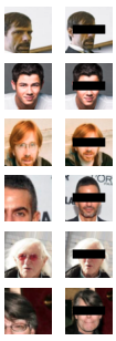
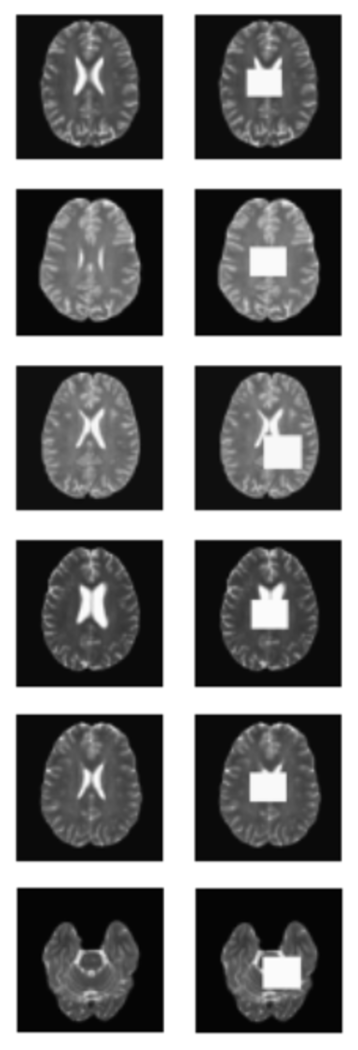
(a) CelebA	(b) IXI

Figure 6: (a) - Left column: anchor image. Right column: augmented image after applying our custom random-erasing transformation. (b) - Left column: anchor image. Right column: augmented image after applying our custom random-erasing transformation.

B.3 MRI Datasets

• IXI IXI dataset comprises 560 pairs of T1 and T2-weighted brain MRI scans. From the 560 pairs, 158 samples are used for testing and the remaining data is divided into 5 folds of 358 training samples and 44 validation samples for cross-validation.

• BraTS21 Menze et al. [2014], Bakas et al. [2017], Baid et al. [2021] dataset comprises 1251 brain MRI scans of four different weightings (T1, T1-CE, T2, FLAIR). The data is split into an unhealthy validation set of 100 samples and an unhealthy test set of 1151 samples.

• MSLUB Lesjak et al. [2018] dataset comprises brain MRI scans of 30 patients with Multiple Sclerosis (MS). For each patient, T1, T2, and FLAIR-weighted scans are available. The data is split into an unhealthy validation set of 10 samples and an unhealthy test set of 20 samples.

Following Behrendt et al. [2024], we utilized T2-weighted images from all datasets across our experiments, as well as performed some pre-processing steps involving brain registration, skull stripping and downsampling. Please refer to Behrendt et al. [2024] for more detailed information on this pre-processing steps.

Appendix C Additional Results

Figure 7 shows the histograms plots of class-label distributions amongst MSE, SSIM and LPIPS on CelebA for the evaluated methods (Diff-AE, SepVAE and Ours).

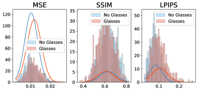
(a) Diff-AE Preechakul et al. [2022]

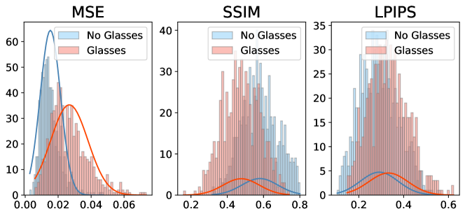
(b) SepVAE Louiset et al. [2023]

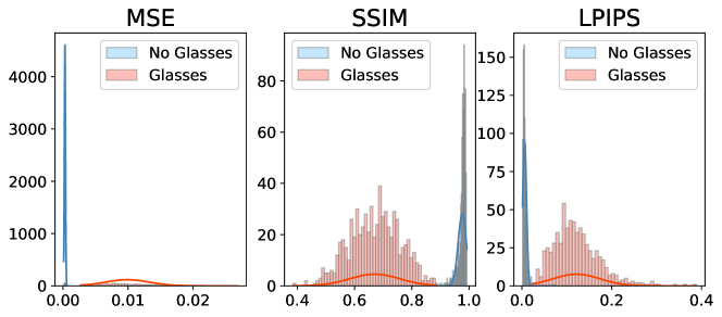
(c) Ours (w/ RE)

Figure 7: Histogram of MSE, SSIM, and LPIPS for CelebA for NEG and EG samples.

The ROC curves on CelebA for MSE, SSIM and LPIPS are illustrated in Figure 8.

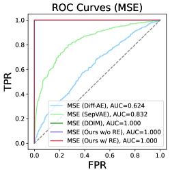
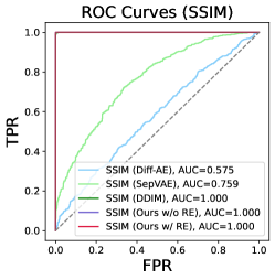
(a) MSE	(b) SSIM	(c) LPIPS

Figure 8: ROC curve on CelebA for (a) MSE, (b) SSIM and (c) LPIPS.

Figure 9 depicts examples of images generated by DDIM using the setp-wise denoining process $p_{\theta}(x_{t-1}|x_{t},z_{bg})$, conditioned on the common latent feature $z_{bg}$.

Figure 9: Identity-conditional generation using the latent representation $z_{bg}$ of the query image. Incorporating random-erasing (RE) during encoder training encourages class-invariance (Section 4.1), as demonstrated by the close-up on the eyes region, where w/o RE the eyes appear uniformly occluded.

Appendix D Ablation Studies

D.1 Sampling Facial Images at Different Timesteps

Figure 10 shows the results for three facial images. We noticed that when choosing a $t>350$, the image gradually loses background (common) information. Conversely, $t<100$ fails to effectively replace eyeglasses, especially if they are sunglasses occluding the eyes (subject of first row). However, for normal eyeglasses without occluding the eyes (subject of last row), $t=100$ proves to be an optimal choice.

Figure 10: Predicted $\textrm{x}_{0}$ at different time steps. The predicted image gradually looses details and is altered as the level of noise increases.

D.2 Instance-alignment and Class-invariant of Common Features Encoder

To assess the influence of $\epsilon$ on both subject identification accuracy and EG/NEG classification accuracy, we conducted an ablation study on $\epsilon$ to verify the instance-alignment and class-invariance properties of our encoder (Section 4.1). The results are reported in Table 4. Specifically, for instance classification, we employed a $k$-NN classifier ($k=3$) and calculated the cosine similarity between the latent representation of each test sample and the remaining test samples. For EG/NEG classification, a logistic regression classifier was trained on the extracted latent features of images to distinguish between EG and NEG examples.

Table 4: Results (Accuracy in %) of Instance Classification and EG/NEG Classification tasks on CelebA.

$\epsilon$	w/o RE		w/ RE
	EG/NEG Class. (%)	Instance Class. (%) ($3-NN$)	EG/NEG Class. (%)	Instance Class. (%) ($3-NN$)
0.0	80.219	24.14	76.715	22.55
0.25	84.599	24.73	74.307	22.80
0.5	82.993	26.32	74.088	22.72
1.0	83.431	25.48	72.336	23.72
1.5	82.555	22.97	72.701	23.05
2.0	84.453	23.47	72.190	23.72
2.5	80.876	24.06	70.949	22.72
3.0	80.657	23.72	71.679	20.54
3.5	80.803	24.48	68.686	21.29
4.0	78.978	22.13	69.270	21.71
4.5	78.467	23.22	68.832	19.87
5.0	77.883	21.71	67.299	20.28
6.0	78.686	23.81	64.161	19.95
7.0	75.036	22.05	62.263	19.20
8.0	73.358	20.54	62.774	20.12
Diff-AE Preechakul et al. [2022] Target Accuracy: 87.664

D.3 Reconstructed Brain MRI images

In Figure 11, the reconstruction version of brain MRIs are depicted for the evaluated methods. Notably, the combination Ours+$p$DDPM achieved the lowest reconstruction $l1$ error. Ablation results on $\epsilon$ are present in Table 5.

Figure 11: Reconstruction results of MRI images using different methods.

Table 5: Ablation results on $\epsilon$ for the combination of our encoder with the evaluated models on brain MRI datasets. The best results are highlighted in bold, and the second-best results are underlined. * denotes that the results were obtained by reproducing the method. The coloured values between brackets indicate the improvement/decrease w.r.t. the correspondent method. The reported results for all metrics correspond to the mean $\pm$ standard deviation across the different folds.

Model	BraTS21		MSLUB		IXI
	DICE (%)$\;\uparrow$	AUPRC (%)$\;\uparrow$	DICE (%)$\;\uparrow$	AUPRC (%)$\;\uparrow$	$l1(1e-3)\downarrow$
AE  Baur et al. [2021]	$32.87$$\pm 1.25$	$31.07$$\pm 1.75$	$7.10$$\pm 0.68$	$5.58$$\pm 0.26$	$30.55$$\pm 0.27$
VAE Baur et al. [2021]	$31.11$$\pm 1.50$	$28.80$$\pm 1.92$	$6.89$$\pm 0.09$	$5.00$$\pm 0.40$	$31.28$$\pm 0.71$
SVAE Behrendt et al. [2022]	$33.32$$\pm 0.14$	$33.14$$\pm 0.20$	$5.76$$\pm 0.44$	$5.04$$\pm 0.13$	$28.08$$\pm 0.02$
DAE Kascenas et al. [2022]	$37.05$$\pm 1.42$	${44.99}$$\pm 1.72$	$3.56$$\pm 0.91$	$5.35$$\pm 0.45$	$10.12$$\pm 0.26$
f-AnoGAN Schlegl et al. [2019]	$24.16$$\pm 2.94$	$22.05$$\pm 3.05$	$4.18$$\pm 1.18$	$4.01$$\pm 0.90$	$45.30$$\pm 2.98$
DDPM* Wyatt et al. [2022]	$39.25$$\pm 1.01$	$47.79$$\pm 1.28$	$5.43$$\pm 1.71$	$7.25$$\pm 0.79$	$14.10$$\pm 1.64$
pDDPM* Behrendt et al. [2024]	$49.47$$\pm 0.91$	$54.68$$\pm 1.02$	$9.17$$\pm 1.29$	10.35$\pm 0.80$	$11.31$$\pm 0.91$
mDDPM* Iqbal et al. [2023]	51.77$\pm 0.18$	$57.49$$\pm 0.41$	$5.03$$\pm 0.37$	$9.47$$\pm 0.02$	$\underline{7.28}$$\pm 0.00$
Ours (Common Features Encoder $+$ DDPM)
$\epsilon=0.5$	$38.68$$\pm 0.85$ (-0.57)	$48.49$$\pm 1.47$ (+0.70)	$6.47$$\pm 1.51$ (+1.04)	$7.69$$\pm 1.30$ (+0.44)	$13.78$$\pm 0.52$ (+0.32)
$\epsilon=1.0$	$39.01$$\pm 0.60$ (-0.24)	$48.01$$\pm 1.30$ (+0.22)	$5.44$$\pm 2.06$ (+0.01)	$7.97$$\pm 0.99$ (+0.72)	$13.85$$\pm 0.60$ (+0.25)
$\epsilon=2.0$	$39.25$$\pm 0.55$ (+0.00)	$48.58$$\pm 1.06$ (+0.79)	$5.39$$\pm 1.13$ (-0.04)	$7.29$$\pm 0.23$ (+0.04)	$13.72$$\pm 0.56$ (+0.38)
$\epsilon=3.0$	$39.21$$\pm 0.36$ (-0.04)	$48.08$$\pm 1.57$ (+0.29)	$5.35$$\pm 1.25$ (-0.08)	$7.38$$\pm 0.81$ (+0.13)	$13.79$$\pm 0.42$ (+0.31)
Ours (Common Features Encoder $+$ pDDPM)
$\epsilon=0.5$	$48.93$$\pm 1.42$ (-0.54)	$54.06$$\pm 1.54$ (-0.62)	10.55$\pm 1.42$ (+1.38)	$9.94$$\pm 0.92$ (-0.41)	$11.15$$\pm 0.01$ (+0.16)
$\epsilon=1.0$	$49.26$$\pm 0.74$ (-0.21)	$54.65$$\pm 0.86$ (-0.03)	$9.29$$\pm 2.25$ (+0.12)	$9.90$$\pm 1.22$ (-0.45)	$11.13$$\pm 0.02$ (+0.18)
$\epsilon=2.0$	$48.84$$\pm 0.61$ (-0.63)	$53.96$$\pm 0.75$ (-0.72)	$9.62$$\pm 0.97$ (+0.45)	$9.71$$\pm 0.44$ (-0.64)	$11.12$$\pm 0.02$ (+0.19)
$\epsilon=3.0$	$49.36$$\pm 0.53$ (-0.11)	$54.60$$\pm 0.60$ (-0.08)	$\underline{10.48}$$\pm 2.19$ (+1.31)	$\underline{10.26}$$\pm 0.67$ (-0.09)	$11.11$$\pm 0.01$ (+0.20)
Ours (Common Features Encoder $+$ mDDPM)
$\epsilon=0.5$	$\underline{51.76}$$\pm 0.85$ (-0.01)	$\underline{57.56}$$\pm 0.96$ (+0.07)	$8.66$$\pm 1.40$ (+3.63)	$9.34$$\pm 1.24$ (-0.13)	$7.36$$\pm 0.00$ (-0.08)
$\epsilon=1.0$	$51.66$$\pm 0.04$ (-0.11)	$57.27$$\pm 0.03$ (-0.22)	$8.69$$\pm 0.33$ (+3.66)	$9.51$$\pm 0.15$ (+0.04)	7.24$\pm 0.79$ (+0.04)
$\epsilon=2.0$	$51.50$$\pm 0.58$ (-0.27)	$57.15$$\pm 0.57$ (-0.34)	$8.75$$\pm 0.96$ (+3.72)	$9.22$$\pm 0.42$ (-0.25)	$7.39$$\pm 0.00$ (-0.11)
$\epsilon=3.0$	$51.69$$\pm 0.17$ (-0.08)	57.58$\pm 0.17$ (+0.09)	$9.47$$\pm 0.18$ (+4.44)	$9.44$$\pm 0.48$ (-0.03)	$7.47$$\pm 0.00$ (-0.19)

Appendix E Potential Impact on Clinical Workflow

The ability to reconstruct normal representations of input images, regardless of the presence of abnormalities, holds considerable significance in the disease diagnosis process. Early detection of diseases is aided by comparing the original image with its reconstructed healthy counterpart. Discrepancies between the images may signify the existence of anomalies or abnormalities, such as tumors. The development of an AI tool designed to assist healthcare practitioners in promptly identifying diseases or abnormalities by comparing two images enables timely intervention and treatment. Additionally, providing clinicians with reconstructed healthy images for comparison purposes can contribute to the reduction of diagnostic errors by providing clearer visualization of abnormalities and assisting in the process of differential diagnosis.

References

- [1] IXI Dataset. URL https://brain-development.org/ixi-dataset/. Accessed: December 6, 2023.
- Abid et al. [2018] Abubakar Abid, Martin J Zhang, Vivek K Bagaria, and James Zou. Exploring patterns enriched in a dataset with contrastive principal component analysis. Nature Communications, 9(1):2134, 2018.
- Baid et al. [2021] Ujjwal Baid, Satyam Ghodasara, Suyash Mohan, Michel Bilello, Evan Calabrese, Errol Colak, Keyvan Farahani, Jayashree Kalpathy-Cramer, Felipe C Kitamura, Sarthak Pati, et al. The RSNA-ASNR-MICCAI BraTS 2021 Benchmark on Brain Tumor Segmentation and Radiogenomic Classification. arXiv preprint arXiv:2107.02314, 2021.
- Bakas et al. [2017] Spyridon Bakas, Hamed Akbari, Aristeidis Sotiras, Michel Bilello, Martin Rozycki, Justin S Kirby, John B Freymann, Keyvan Farahani, and Christos Davatzikos. Advancing The Cancer Genome Atlas glioma MRI collections with expert segmentation labels and radiomic features. Scientific Data, 4(1):1–13, 2017.
- Barbano et al. [2023] Carlo Alberto Barbano, Benoit Dufumier, Enzo Tartaglione, Marco Grangetto, and Pietro Gori. Unbiased supervised contrastive learning. In The Eleventh International Conference on Learning Representations (ICLR), 2023. URL https://openreview.net/forum?id=Ph5cJSfD2XN.
- Baur et al. [2021] Christoph Baur, Stefan Denner, Benedikt Wiestler, Nassir Navab, and Shadi Albarqouni. Autoencoders for unsupervised anomaly segmentation in brain MR images: a comparative study. Medical Image Analysis, 69:101952, 2021.
- Behrendt et al. [2022] Finn Behrendt, Marcel Bengs, Debayan Bhattacharya, Julia Krüger, Roland Opfer, and Alexander Schlaefer. Capturing inter-slice dependencies of 3D brain MRI-scans for unsupervised anomaly detection. In Proceedings of the Medical Imaging with Deep Learning, 2022.
- Behrendt et al. [2024] Finn Behrendt, Debayan Bhattacharya, Julia Krüger, Roland Opfer, and Alexander Schlaefer. Patched Diffusion Models for Unsupervised Anomaly Detection in Brain MRI. In Proceedings of the International Conference on Medical Imaging with Deep Learning (MIDL), pages 1019–1032. PMLR, 2024.
- Bishop and Bishop [2024] Christopher M. Bishop and Hugh Bishop. Deep Learning: Foundations and Concepts. Springer, 2024.
- Carton et al. [2024] Florence Carton, Robin Louiset, and Pietro Gori. Double InfoGAN for Contrastive Analysis. arXiv preprint arXiv:2401.17776, 2024.
- Chen et al. [2020] Ting Chen, Simon Kornblith, Mohammad Norouzi, and Geoffrey Hinton. A Simple Framework for Contrastive Learning of Visual Representations. In International Conference on Machine Learning, pages 1597–1607. PMLR, November 2020. URL http://proceedings.mlr.press/v119/chen20j.html. ISSN: 2640-3498.
- Dhariwal and Nichol [2021] Prafulla Dhariwal and Alexander Nichol. Diffusion Models Beat GANs on Image Synthesis. Advances in Neural Information Processing Systems, 34:8780–8794, 2021.
- Dufumier et al. [2023] Benoit Dufumier, Carlo Alberto Barbano, Robin Louiset, Edouard Duchesnay, and Pietro Gori. Integrating prior knowledge in contrastive learning with kernel. In 40 th International Conference on Machine Learning (ICML), 2023.
- Hadsell et al. [2006] R. Hadsell, S. Chopra, and Y. LeCun. Dimensionality Reduction by Learning an Invariant Mapping. In CVPR, volume 2, pages 1735–1742. IEEE, 2006.
- Ho et al. [2020] Jonathan Ho, Ajay Jain, and Pieter Abbeel. Denoising Diffusion Probabilistic Models. Advances in Neural Information Processing Systems, 33:6840–6851, 2020.
- Iqbal et al. [2023] Hasan Iqbal, Umar Khalid, Chen Chen, and Jing Hua. Unsupervised Anomaly Detection in Medical Images Using Masked Diffusion Model. In Proceedings of the International Workshop on Machine Learning in Medical Imaging (MLMI), pages 372–381. Springer, 2023.
- Kascenas et al. [2022] Antanas Kascenas, Nicolas Pugeault, and Alison Q O’Neil. Denoising autoencoders for unsupervised anomaly detection in brain MRI. In Proceedings of the International Conference on Medical Imaging with Deep Learning (MIDL), pages 653–664, 2022.
- Khosla et al. [2020] Prannay Khosla, Piotr Teterwak, Chen Wang, Aaron Sarna, Yonglong Tian, Phillip Isola, Aaron Maschinot, Ce Liu, and Dilip Krishnan. Supervised contrastive learning. volume 33, pages 18661–18673. Curran Associates, Inc., 2020. URL https://proceedings.neurips.cc/paper/2020/file/d89a66c7c80a29b1bdbab0f2a1a94af8-Paper.pdf.
- Lesjak et al. [2018] Žiga Lesjak, Alfiia Galimzianova, Aleš Koren, Matej Lukin, Franjo Pernuš, Boštjan Likar, and Žiga Špiclin. A novel public MR image dataset of multiple sclerosis patients with lesion segmentations based on multi-rater consensus. Neuroinformatics, 16:51–63, 2018.
- Liu et al. [2015] Ziwei Liu, Ping Luo, Xiaogang Wang, and Xiaoou Tang. Deep learning face attributes in the wild. In Proceedings of International Conference on Computer Vision (ICCV), December 2015.
- Louiset et al. [2023] Robin Louiset, Edouard Duchesnay, Antoine Grigis, Benoit Dufumier, and Pietro Gori. SepVAE: a contrastive VAE to separate pathological patterns from healthy ones. arXiv preprint arXiv:2307.06206, 2023.
- Menze et al. [2014] Bjoern H Menze, Andras Jakab, Stefan Bauer, Jayashree Kalpathy-Cramer, Keyvan Farahani, Justin Kirby, Yuliya Burren, Nicole Porz, Johannes Slotboom, Roland Wiest, et al. The Multimodal Brain Tumor Image Segmentation Benchmark (BRATS). IEEE Transactions on Medical Imaging, 34(10):1993–2024, 2014.
- Oord et al. [2019] Aaron van den Oord, Yazhe Li, and Oriol Vinyals. Representation Learning with Contrastive Predictive Coding. arXiv:1807.03748 [cs, stat], January 2019. URL http://arxiv.org/abs/1807.03748. arXiv: 1807.03748.
- Patrício et al. [2023] Cristiano Patrício, João C Neves, and Luís F Teixeira. Explainable Deep Learning Methods in Medical Image Classification: A Survey. ACM Computing Surveys, 56(4):1–41, 2023.
- Preechakul et al. [2022] Konpat Preechakul, Nattanat Chatthee, Suttisak Wizadwongsa, and Supasorn Suwajanakorn. Diffusion Autoencoders: Toward a Meaningful and Decodable Representation. In Proceedings of the IEEE/CVF Conference on Computer Vision and Pattern Recognition (CVPR), pages 10619–10629, 2022.
- Ronneberger et al. [2015] Olaf Ronneberger, Philipp Fischer, and Thomas Brox. U-Net: Convolutional Networks for Biomedical Image Segmentation. In Proceedings of the Medical Image Computing and Computer-Assisted Intervention (MICCAI), pages 234–241. Springer, 2015.
- Schlegl et al. [2019] Thomas Schlegl, Philipp Seeböck, Sebastian M Waldstein, Georg Langs, and Ursula Schmidt-Erfurth. f-AnoGAN: Fast unsupervised anomaly detection with generative adversarial networks. Medical Image Analysis, 54:30–44, 2019.
- Schroff et al. [2015] Florian Schroff, Dmitry Kalenichenko, and James Philbin. Facenet: A unified embedding for face recognition and clustering. In Proceedings of the IEEE conference on computer vision and pattern recognition, pages 815–823, June 2015. doi: 10.1109/CVPR.2015.7298682. URL http://arxiv.org/abs/1503.03832. arXiv: 1503.03832.
- Song et al. [2021] Jiaming Song, Chenlin Meng, and Stefano Ermon. Denoising Diffusion Implicit Models. In Proceedings of the International Conference on Learning Representations (ICLR), 2021.
- Tian et al. [2020] Yonglong Tian, Dilip Krishnan, and Phillip Isola. Contrastive Multiview Coding. In Andrea Vedaldi, Horst Bischof, Thomas Brox, and Jan-Michael Frahm, editors, Computer Vision – ECCV 2020, Lecture Notes in Computer Science, pages 776–794, Cham, 2020. Springer International Publishing. ISBN 978-3-030-58621-8. doi: 10.1007/978-3-030-58621-8_45. tex.ids= tian_contrastive_2020 arXiv: 1906.05849.
- Wang et al. [2004] Zhou Wang, A.C. Bovik, H.R. Sheikh, and E.P. Simoncelli. Image quality assessment: from error visibility to structural similarity. IEEE Transactions on Image Processing, 13(4):600–612, 2004.
- Weinberger et al. [2022] Ethan Weinberger, Nicasia Beebe-Wang, and Su-In Lee. Moment matching deep contrastive latent variable models. arXiv preprint arXiv:2202.10560, 2022.
- Wyatt et al. [2022] Julian Wyatt, Adam Leach, Sebastian M. Schmon, and Chris G. Willcocks. AnoDDPM: Anomaly Detection with Denoising Diffusion Probabilistic Models using Simplex Noise. In Proceedings of the IEEE/CVF Conference on Computer Vision and Pattern Recognition Workshops (CVPRW), pages 649–655, 2022.
- Zhang et al. [2018] Richard Zhang, Phillip Isola, Alexei A Efros, Eli Shechtman, and Oliver Wang. The unreasonable effectiveness of deep features as a perceptual metric. In Proceedings of the IEEE Conference on Computer Vision and Pattern Recognition (CVPR), pages 586–595, 2018.
- Zhong et al. [2020] Zhun Zhong, Liang Zheng, Guoliang Kang, Shaozi Li, and Yi Yang. Random Erasing Data Augmentation. In Proceedings of the AAAI Conference on Artificial Intelligence, volume 34, pages 13001–13008, 2020.
- Zou et al. [2013] James Y Zou, Daniel J Hsu, David C Parkes, and Ryan P Adams. Contrastive Learning Using Spectral Methods. Advances in Neural Information Processing Systems, 26, 2013.