Ensemble Deep Random Vector Functional Link Neural Network Based on Fuzzy Inference System
Abstract
The ensemble deep random vector functional link (edRVFL) neural network has demonstrated the ability to address the limitations of conventional artificial neural networks. However, since edRVFL generates features for its hidden layers through random projection, it can potentially lose intricate features or fail to capture certain non-linear features in its base models (hidden layers). To enhance the feature learning capabilities of edRVFL, we propose a novel edRVFL based on fuzzy inference system (edRVFL-FIS). The proposed edRVFL-FIS leverages the capabilities of two emerging domains, namely deep learning and ensemble approaches, with the intrinsic IF-THEN properties of fuzzy inference system (FIS) and produces rich feature representation to train the ensemble model. Each base model of the proposed edRVFL-FIS encompasses two key feature augmentation components: a) unsupervised fuzzy layer features and b) supervised defuzzified features. The edRVFL-FIS model incorporates diverse clustering methods (R-means, K-means, Fuzzy C-means) to establish fuzzy layer rules, resulting in three model variations (edRVFL-FIS-R, edRVFL-FIS-K, edRVFL-FIS-C) with distinct fuzzified features and defuzzified features. Within the framework of edRVFL-FIS, each base model utilizes the original, hidden layer and defuzzified features to make predictions. Experimental results, statistical tests, discussions and analyses conducted across UCI and NDC datasets consistently demonstrate the superior performance of all variations of the proposed edRVFL-FIS model over baseline models.
Index Terms:
Ensemble Learning, Deep Learning, Random Vector Functional Link (RVFL) Network, Ensemble Deep RVFL, Fuzzy Inference System, Big Data.I Introduction
The efficacy of neural network-based models stems from their ability to discern intricate latent patterns within input and output vectors, leveraging their inherent ability to capture complex relationships in data. This attribute facilitates superior learning and predictive capabilities in diverse applications such as in health care [1], stock market predictions [2], Alzheimer’s disease diagnosis [3], solving mathematical differential equations [4] and so on.
Neural networks (NNs) aim to discover a hypothesis function, denoted as , within the hypothesis space , to effectively approximate a target function defined on a domain . The primary objective in learning is to minimize generalization error by closely aligning the approximation with the true, albeit unknown, function. serves as a mapping from input space to corresponding target labels or classes. Mathematically, , where and are the input and output vectors, respectively. The set encompasses the learning parameters associated with the hypothesis function . The accuracy of the hypothesis in approximating the real function is contingent upon the efficacy of determining/computing the parameters .
In traditional NNs, the backpropagation (BP) algorithm iteratively seeks to optimize model parameters () by comparing predicted outputs to true outputs. However, in BP-based NNs, several challenges arise during the training process, such as potential slowness, susceptibility to local optima [5], and the critical influence of factors such as learning rate and initialization point. Training conventional NNs on large datasets demands significant computational resources and time due to the gradient-based iterative process of the BP algorithm.
Randomized NNs (RNNs) [6], introduced as an alternative to BP-based NNs, address the abovementioned limitations of conventional NNs. In RNNs, certain parameters are fixed during the training process, and the output layer’s parameters are calculated using an iterative process or closed-form solution. The random vector functional link (RVFL) neural network [7, 8] is a shallow feed-forward RNN characterized by randomly initialized hidden layer parameters that remain fixed throughout the training process. RVFL distinguishes itself from other RNNs through direct link incorporation between input and output layers. Direct links enhance the learning performance of the RVFL by behaving as an implicit regularization technique [9, 10]. Utilizing the Pseudo-inverse or least-squares approach, RVFL provides a closed-form solution to determine optimal output parameters, demonstrating universal approximation capability [11]. This methodology minimizes the need for extensive computational resources, offering efficient learning with fewer adjustable settings.
The shallow RVFL model is associated with certain limitations, notably an unstable classifier [12], and its reliance on a single hidden layer hinders its ability to effectively capture the intricate hidden relationships present in the data. To overcome those limitations, within the standard RVFL model, notable enhancements have been implemented using two distinct research frameworks: ensemble learning [13] and deep learning [14]. Shi et al. [15] proposed deep RVFL (dRVFL) and ensemble dRVFL (edRVFL) networks. The dRVFL introduces a deep architecture that can accommodate multiple hidden layers and captures complex relationships within the dataset. The edRVFL network is based on implicit ensemble learning and leverages each hidden layer as a classifier to form an ensemble. The incorporation of multiple RVFL models (base models) within the edRVFL framework enhances its stability and effectiveness compared to the shallow RVFL model.
Over the years, several variants based on the edRVFL architecture have been developed. The original edRVFL lacks provisions for online learning. Recognizing this gap, Gao et al. [16] introduced the dynamic edRVFL, a variant that introduces three crucial online components: online decomposition, online training, and online dynamic ensemble. In the field of cognitive research, Li et al. [17] proposed the spectral-edRVFL (SedRVFL) network, which specializes in feature learning from electroencephalogram (EEG) data to enhance passive brain-computer interface (pBCI) classification tasks. In [18], authors focused on medical imaging, where they combined magnetic resonance imaging (MRI) and positron emission tomography (PET) scans using a convolutional neural network (CNN) and an ensemble of non-iterative RVFL models for diagnosing Alzheimer’s disease. Cheng et al. [19] contributed an edRVFL variant tailored for predictive analytics, specifically in the context of ship order book dynamics. He et al. [20] presented the model-embedded self-supervised edRVFL (ME-SedRVFL) network for underwater signal processing, particularly in estimating the direction-of-arrival (DOA) of acoustic signals. These advancements underscore the versatility of the edRVFL model across various domains, ranging from cognitive neuroscience to signal processing.
Fuzzy logic [21] represents a mathematical approach that addresses uncertain and imprecise information nuances. Within this framework, fuzzy inference system (FIS) [22] is a computational model employing fuzzy logic principles. The FIS operates by integrating fuzzy sets, linguistic variables, and a set of rules to emulate human-like IF-THEN reasoning [23]. Its fundamental components include fuzzification, rule evaluation, and defuzzification [24]. In the fuzzification phase, precise input values are transformed into fuzzy sets. Rule evaluation involves applying a set of conditional statements expressed in linguistic terms to generate fuzzy output values. The subsequent defuzzification process converts these fuzzy outputs into precise and actionable outcomes. FIS finds applications across diverse domains, including control systems [25], pattern identification [26], finance [27], weather forecasting [28], classification [23, 24] and so on.
The performance of NN-based models heavily relies on the generation of hidden layers’ features, which influence the subsequent propagation of information to the output layers. Since the edRVFL generates its hidden layers’ features through random projection, therefore, certain salient features may be lost during hidden layer formation, or some non-linear features may got uncaptured by the edRVFL’s base models (hidden layers). The studies suggest that the augmentation of feature enhancement in RVFL-based variants [29, 30, 31] markedly enhances their performance by capturing nuanced patterns and relationships in the data. However, the feature enhancement techniques remain largely unexplored in the context of edRVFL-based models.
Motivated by the successful implementation of feature enhancement techniques in RVFL-based models and considering the dynamic nature of feature enhancement capability of FIS through the generation of the number of fuzzy centres, as many as necessary (refer to Section III), to facilitate the learning process and improve the model’s overall effectiveness; we propose an ensemble deep RVFL based on a fuzzy inference system (edRVFL-FIS). Within this architecture, input samples traverse a fuzzy layer employing fuzzification. Subsequently, the original input features are concatenated with fuzzy features, forming an extended feature layer and contributing to the generation of hidden layers’ features. Each base model utilizes both the hidden layers and defuzzified features (obtained through the defuzzification process) to make predictions. This ensemble framework leverages the synergy between deep learning and fuzzy logic to enhance the model’s capacity to capture intricate patterns in the data.
As the fuzzy layer is constructed based on fuzzy rule centers, and it interacts with hidden layers and defuzzified layer, the significance of fuzzy centers becomes evident in the generation of hidden features of the proposed edRVFL-FIS model. Thus, it can be inferred that different clustering techniques excel in distinct scenarios, contributing to the overall versatility and effectiveness of the proposed edRVFL-FIS model. Therefore, we propose three variants of the edRVFL-FIS model by incorporating diverse clustering approaches—randomly initialized centers (R-means), K-means, and Fuzzy C-means—to establish fuzzy layer centers. This yields three model variations, namely, edRVFL-FIS-R, edRVFL-FIS-K, and edRVFL-FIS-C, respectively.
The paper’s key highlights are as follows:
-
1.
We propose the edRVFL-FIS model, in which each hidden layer’s features are generated on the ground of enhanced feature space (obtained through the concatenation of original and fuzzy features).
-
2.
Each base model of the proposed edRVFL-FIS comprises two main feature enhancement components: a) unsupervised fuzzy layer feature and b) supervised defuzzified features.
-
3.
We propose three variants of the proposed edRVFL-FIS models, namely, edRVFL-FIS-R, edRVFL-FIS-K, and edRVFL-FIS-C based on R- means, K-means, and Fuzzy C-means clustering techniques for fuzzy layer generation. Thus, each variant generates distinct sets of fuzzified and defuzzified features. These assorted combinations enhance the overall performance of the edRVFL-FIS model.
-
4.
The ensemble structure of the proposed edRVFL-FIS utilizes diverse defuzzified features for each base model, capitalizing on inherent diversity. This enables rich feature extraction in the output prediction process by leveraging original, hidden, and defuzzified features.
-
5.
The performance evaluation of the proposed edRVFL-FIS model involves testing on benchmark UCI datasets originating from diverse domains and exhibiting varying sizes against existing baseline models. Additionally, experiments are conducted on NDC datasets to demonstrate the effectiveness of the proposed model for big data.
The succeeding sections of this paper are structured as follows: Section II introduces RVFL, edRVFL, and the Takagi-Sugeno-Kang (TSK) neuro-fuzzy inference system. Section III details the mathematical framework of the proposed edRVFL-FIS model. Experimental results and statistical analyses of proposed and existing models are discussed in Section IV. The discussions based on the empirical findings are done in Section V with conclusive remarks and future research directions provided in Section VI.
II Related Works
Before delving into the structure and mathematical framework of the proposed edRVFL-FIS model, it is necessary to go through the mathematical frameworks of RVFL and edRVFL models to establish a foundational knowledge base. Additionally, defining the Takagi-Sugeno-Kang (TSK) FIS is crucial as it forms the core component in our proposed edRVFL-FIS model (refer to Section III). Thus, firstly, we fix some notations and discuss the framework of RVFL (in Section S.I of the supplementary material) and edRVFL, followed by the TSK fuzzy systems.
II-A Notations
Let be the total number of training samples. Let and be the collection of all input and target vectors, and , respectively, for . Then and , where is the transpose operator. denotes the number of hidden
layers, and denotes the number of hidden layer nodes. and denote the Kronecker product and the Concatenation operator, respectively and are defined below. For , and , then and
II-B Ensemble Deep RVFL (edRVFL) [15]
Derived from the principles of deep representation learning, the deep RVFL (dRVFL) represents an advancement of the shallow RVFL structure. This extension involves stacking multiple enhancement layers, creating a framework for profound representation learning. Each enhancement layer processes the input features to guide the generation of random features, fostering the creation of a varied feature set through hierarchical structures. By integrating ensemble learning into the architecture of dRVFL, ensemble deep RVFL (edRVFL) was proposed, leveraging both ensemble and deep learning frameworks. Diverging from common deep learning models characterized by a single output layer, the edRVFL undertakes the training of multiple output layers, utilizing all hidden layers to create a base model.
In an edRVFL network comprising enhancement layers, each layer contains enhancement nodes. Let the hidden matrix of the layer be denoted as , for . is calculated as:
| (1) |
where is the randomly initialized weights matrix, , is the bias vector and is the activation function. is calculated as:
| (2) |
Here, denotes the weights matrix and the bias vector in the layer. The enhancement features, formed by concatenating the input and hidden features, serve as input to the respective output layer. The calculation of follows the identical procedure used in RVFL. The classification is attained by consolidating the outcomes from all base models (hidden layers) through averaging or majority voting methods.
II-C Takagi-Sugeno-Kang (TSK) Neuro-Fuzzy Inference System (FIS) [32]
The TSK neuro-FIS [32] is an efficacious approach for modeling intricate systems in uncertainty. TSK exhibits the ability to capture nonlinear relationships transparently through the amalgamation of fuzzy sets, fuzzy rules, and local linear models. Its broad applicability and practicality render it a widely adopted choice in diverse real-world scenarios in the realms of fuzzy logic and deep learning [33]. The TSK operates on a collection of IF-THEN fuzzy rules and is commonly formulated as:
where is a fuzzy set, is the system input (), and is the number of fuzzy rules. Here, the function in a fuzzy system is often described as any relevant function capable of properly describing the output within the given range of fuzzy rules. Nevertheless, in practical terms, is presumed to take the form of a linear polynomial in the input variables within the context of a fuzzy system. The rule’s fire strength is calculated as:
| (3) |
where is the membership function corresponding to the
fuzzy set .
The defuzzification of the TSK model is carried out as follows:
| (4) |
The above-discussed related works not only enhance our understanding of existing models but also pave the way for proposing the edRVFL-FIS model.
III The Proposed Ensemble Deep RVFL Based on a Fuzzy Inference System (RVFL-FIS)
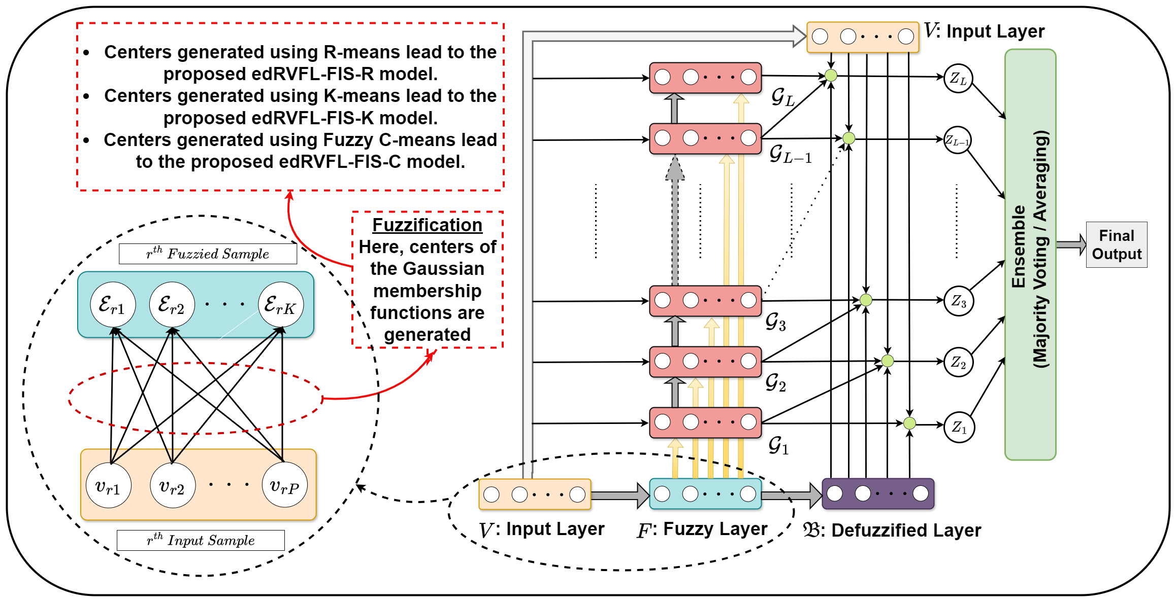
In this section, we fuse the fuzzy inference system, (i.e., TSK) with the edRVFL structure and propose a hybrid edRVFL-FIS model that has a reach feature representation. The architecture of the proposed edRVFL-FIS is represented in Figure 1. In the edRVFL-FIS model, input samples undergo a fuzzification process and form a fuzzy layer. Further, the generation of a defuzzified layer takes place via the defuzzification process. The subsequent hidden layer is formed by the input, fuzzified, and preceding hidden layers (except for the first hidden layer), utilizing random projection. Each hidden layer within the model operates as an autonomous base model (RVFL). We refer to the hidden layer features, original input features, and defuzzified features collectively as enhanced fuzzified features. The sample with enhanced features for the base model serves as an input and propagates to the output layer of the model. Each base model within the edRVFL-FIS framework behaves as RVFL models that incorporate distinct input features. This architecture of the proposed edRVFL-FIS allows for a structured and modular processing of data, where each hidden layer operates as its own self-contained model within the larger network architecture. Moreover, the ensemble structure leverages diverse supervised defuzzified features for each base model, enhancing richness in feature extraction during output prediction.
First of all, we describe the general structure of the proposed edRVFL-FIS model, and then the subsequent subsections discuss the method of fuzzification and defuzzification, which will be incorporated in the proposed edRVFL-FIS model for feature enhancement.
III-A Proposed Model: A Framework
Suppose denotes the total number of fuzzy rules in the fuzzy layer. Let be the fuzzy layer’s matrix and be the defuzzified matrix corresponding to all the training samples.
Hidden layer formations and their corresponding outputs:
hidden layer and output: The training input matrix and the fuzzified matrix traverse the first hidden layer, , through random projection followed by non-linear transformation by employing the activation function . Therefore
| (5) |
where and are the randomly generated weight matrix and bias vector, respectively, for the hidden layer. The first hidden layer generates the first base model for the ensembling. The enhancement features (formed by the input, hidden, and defuzzified features) serve as input to the first output layer. Therefore, the first layer’s output matrix is defined as:
| (6) |
where is the unknown weight matrix connecting the input layer and the hidden layer to the output layer and .
hidden layer and output for : The training input matrix , the previous hidden layer’s matrix and the fuzzified samples matrix traverse the hidden layer, . Therefore,
| (7) |
where and are the randomly generated hidden layer weight matrix and bias vector, respectively, for the hidden layer. The hidden layer behaves as a base model (RVFL) and the corresponding output matrix is defined as:
| (8) |
where is the unknown weight matrix connecting the input layer and the hidden layer to the output layer and .
The anticipated output matrices ’s (for ) are combined through majority voting or averaging to find the final predicted output. However, how to find the fuzzy layer’s matrix , the defuzzified matrix , and the weights matrix connecting the base models (hidden layers) to the output layer remains to answer. We discuss answers to the aforementioned questions in the subsequent subsections.
III-B Fuzzification Process for the Proposed Model
The proposed edRVFL-FIS model uses fuzzified matrix into the generation of the hidden layer process. Therefore, each and every training sample is fuzzified using the TSK FIS. For this, let be the fuzzy set with the membership function of component of fuzzy rule of the fuzzy layer, where , .
then, by considering the first-order TSK fuzzy system, we get
Here are the randomly generated coefficients.
The weighted fire strength of the fuzzy rule in the fuzzy layer is given as:
| (9) |
In our work, we consider the Gaussian membership function within fuzzy sets of the fuzzy layer. The membership value of for the fuzzy rule is defined as :
| (10) |
where is the center and is the standard deviation in the fuzzy rule. The number of fuzzy rules in the fuzzy layer is equal to the number of centers.
In the proposed edRVFL-FIS model, we generate the centers in the fuzzy layer using three different clustering methods, which are:
-
1.
Randomly initialized centers (say R-means).
-
2.
Using K-means clustering.
-
3.
Using Fuzzy C-means clustering.
Remark: Three distinct variants of edRVFL-FIS arise from the application of three different center initialization approaches, thereby enhancing the diversity within our proposed model. The variations of the proposed edRVFL-FIS initialized with R-means, K-means, and Fuzzy C-means clustering techniques are denoted as edRVFL-FIS-R, edRVFL-FIS-K, and edRVFL-FIS-C, respectively.
Now, the unsupervised fuzzified vector of the training sample is given as:
| (11) |
The fuzzified matrix corresponding to the input matrix is given as:
| (12) |
III-C Defuzzification Process for the Proposed Model
Here, we articulate the defuzzification process for the fuzzified vectors. This process enables the defuzzified output from the fuzzy layer of our proposed edRVFL-FIS model to contribute to the anticipation of the final output layers alongside the original features (via direct links) and the hidden layers. Since the target matrix has classes, therefore the output of each fuzzy layer must have features. The defuzzified output of the sample is defined as follows:
| (13) |
where , and is the parameter
used in THEN part of the fuzzy inference system used in the proposed edRVFL-FIS model. ’s are the unknown parameters and are calculated along with the output layer weights of the edRVFL-FIS model in the subsection III-D. Therefore, for the input matrix , the defuzzified matrix is given as:
| (14) |
| (15) |
Here represents the componentwise matrix multiplication,
| (16) |
III-D Output Layers Parameters for Each Base Model of the Proposed Model
To get the output of the base models, we put the value of from Eq. (15) in (6) and (8), we get
| (17) |
| (18) | ||||
| (19) |
Here, if and if .
To get the output of each base model of the edRVFL-FIS, is the matrix of unknowns that need to be found. The resultant optimization problem of Eq. (17) is given as:
| (20) |
The weight matrix is computed as follows:
| (21) |
where is an identity matrix of conformal dimension.
III-E Final Output: Test Condition
For an unknown sample , the output of the base model is
| (22) |
The base model outputs, , are combined using majority voting to get the final output as follows:
| (23) |
where is the indicator function that evaluates to if , and otherwise.
III-F Further Takeaways from the Defuzzification Matrix of the Proposed Model
Let denote the number of rows in the matrix , be a matrix of dimension with all the entries equal zero and as an identity matrix of dimension . Since,
| (24) |
multiplying (from left) both sides by the matrix , we get
| (25) |
Eq. (25) implies that the matrix holds distinct values for each base model (hidden layer ) within the ensemble, emphasizing the uniqueness of each model’s contribution. The ensemble structure strategically harnesses the diverse supervised defuzzified matrices across multiple base models, capitalizing on the inherent diversity embedded within the proposed edRVFL-FIS model. Consequently, the proposed edRVFL-FIS demonstrates rich feature extraction capability achieved by leveraging original (through direct link), hidden layer, and defuzzified features.
Source code link: https://github.com/mtanveer1/edRVFL-FIS.
III-G Time and Space Complexity of the Proposed edRVFL-FIS Models
The complexity of the proposed edRVFL-FIS models primarily depends on two components: (a) clustering technique and (b) requirement of matrix inversion in (21).
The number of hidden layers for the edRVFL-FIS has taken (see Section S.II of the supplementary materials), which is very small compared to other variables; therefore, we generally do not give much attention to in the computational complexity.
Time/Temporal Complexity: Following [34], the time complexity of K-means and Fuzzy C-means are and , respectively, where “” represents the number of iterations. The time complexity of R-means is . Following [15], time complexity in computing inverse in (21) is , where if or if . Therefore, total time complexity for edRVFL-FIS-R, edRVFL-FIS-K, and edRVFL-FIS-C are , and , respectively.
Space/Spatial Complexity: Following [35], the space complexity of Fuzzy C-means is and the space complexity of K-means and R-means is .
Following [15], space complexity in computing inverse in (21) is , where if or if . Therefore, total space complexity for edRVFL-FIS-R, edRVFL-FIS-K, and edRVFL-FIS-C are , and , respectively.
IV Experiments and Results
The section presents comprehensive details on the datasets, the compared models, and the experimental configuration in Section S.II of the supplementary material. Subsequently, we delve into the experimental results and conduct statistical analyses on both UCI and NDC datasets. Finally, we examine the influence of fuzzy rules, hidden layers and robustness of the proposed edRVFL-FIS models.
IV-A Datasets
To evaluate the efficacy of the proposed edRVFL-FIS models, we employ datasets from UCI [36] and NDC [37]. We categorize UCI datasets into two groups: Category-1 with sample sizes ranging from 100 to 1000, and Category-2 with sample sizes between 1000 and 10000. These datasets span diverse domains and sizes, with detailed statistics provided in supplementary Tables S.IV and S.V. The NDC dataset, generated using David Musicant’s NDC Data Generator [37], spans from 10 thousand to 1 million samples, consistently featuring 32 features.
IV-B Compared Models
We compare the proposed edRVFL-FIS models with eight baseline and state-of-the-art RNN-based models. The enumerated models under examination include:
-
1.
RVFL: Standard shallow RVFL model [7].
-
2.
ELM: Standard shallow ELM model [38].
-
3.
BLS: Broad learning system [39].
-
4.
H-ELM: Hierarchical ELM model [40].
-
5.
dRVFL: Deep RVFL model [15].
-
6.
edRVFL: Ensemble deep RVFL model [15].
-
7.
Fuzzy BLS: Neuro-Fuzzy-based BLS model [41].
-
8.
edEGERVFL: Ensemble deep extended graph embedded RVFL [42].
-
9.
edRVFL-FIS-R: The proposed ensemble deep RVFL based on FIS with R-means clustering.
-
10.
edRVFL-FIS-K: The proposed ensemble deep RVFL based on FIS with K-means clustering.
-
11.
edRVFL-FIS-C: The proposed ensemble deep RVFL based on FIS with fuzzy C-means clustering.
IV-C Experimental Results, Discussions and Statistical Analysis on Category-1 UCI Dataset
| Dataset Model | RVFL [7] | ELM [38] | BLS [39] | H-ELM [40] | dRVFL [15] | edRVFL [15] | Fuzzy BLS [41] | edEGERVFL [42] | edRVFL-FIS-R† | edRVFL-FIS-K† | edRVFL-FIS-C† |
|---|---|---|---|---|---|---|---|---|---|---|---|
| balance_scale | 98.24 | 98.24 | 98.08 | 91.68 | 95.68 | 95.36 | 98.4 | 97.76 | 98.56 | 98.56 | 98.88 |
| breast_cancer_wisc | 89.4193 | 89.7061 | 87.703 | 87.5622 | 87.9887 | 87.8458 | 91.1367 | 89.1326 | 89.8489 | 89.4234 | 89.8479 |
| dermatology | 96.9974 | 97.264 | 97.8119 | 97.264 | 96.99 | 97.2677 | 97.5454 | 96.9937 | 97.5417 | 97.8082 | 97.8156 |
| echocardiogram | 83.9031 | 83.9031 | 86.2108 | 84.6724 | 84.6724 | 84.6724 | 81.6239 | 80.114 | 86.9801 | 86.2108 | 86.2108 |
| ecoli | 60.6146 | 60.9131 | 60.9175 | 59.4293 | 60.3205 | 61.2116 | 60.0176 | 56.734 | 61.5101 | 60.9131 | 61.216 |
| energy_y1 | 88.4034 | 88.5341 | 88.2828 | 88.2718 | 89.5807 | 90.3591 | 89.3209 | 88.6741 | 91.9226 | 92.3173 | 92.3164 |
| energy_y2 | 91.1451 | 91.6645 | 89.8413 | 88.0129 | 90.6222 | 90.494 | 91.4048 | 87.6292 | 92.3164 | 92.1857 | 92.5787 |
| flags | 52.6046 | 51.5924 | 53.6437 | 53.1309 | 53.1174 | 52.0648 | 52.6451 | 56.1673 | 54.143 | 54.6829 | 54.6559 |
| heart_switzerland | 44.8667 | 46.4333 | 48.1333 | 44.0667 | 44.8 | 43.2 | 44.8 | 50.4667 | 49.7 | 47.3667 | 47.3333 |
| iris | 65.3333 | 65.3333 | 76 | 62.6667 | 74 | 72 | 71.3333 | 74.6667 | 74.6667 | 76 | 76 |
| led_display | 72.7 | 72.6 | 72.1 | 73.4 | 72.3 | 72.3 | 73.1 | 71.9 | 72.9 | 73.2 | 73.1 |
| lymphography | 84.3908 | 84.4138 | 85.7241 | 86.4598 | 85.7241 | 83.7241 | 85.7011 | 85.7931 | 87.1264 | 87.0805 | 86.4138 |
| mammographic | 79.7134 | 79.0906 | 78.6739 | 78.3609 | 79.9196 | 79.3998 | 79.9207 | 79.3998 | 79.9212 | 80.231 | 80.2315 |
| pittsburg_bridges_REL_L | 59.0476 | 63.1905 | 64.1429 | 51.8095 | 64.2381 | 61.4286 | 63.381 | 75.2381 | 72.9524 | 69 | 64.0952 |
| pittsburg_bridges_T_OR_D | 86.1429 | 86.1429 | 90.1429 | 86.1429 | 86.1429 | 86.1429 | 89.1429 | 91.1429 | 90.1905 | 86.1429 | 89.1429 |
| statlog_heart | 80.7407 | 80.7407 | 82.2222 | 79.6296 | 81.4815 | 81.8519 | 81.1111 | 80.7407 | 81.8519 | 83.3333 | 83.3333 |
| statlog_vehicle | 81.6777 | 82.032 | 82.3871 | 78.7219 | 82.7428 | 82.1504 | 78.8402 | 79.9053 | 82.2694 | 82.7421 | 83.5698 |
| tic_tac_toe | 89.9651 | 91.0046 | 97.5982 | 65.3125 | 99.0587 | 99.0581 | 82.4493 | 99.0581 | 99.1623 | 98.3257 | 99.3717 |
| zoo | 92 | 93 | 96 | 92 | 94 | 94 | 95 | 96 | 96 | 95 | 96 |
| Average Accuracy | 78.8371 | 79.2526 | 80.8219 | 76.2418 | 80.1779 | 79.7122 | 79.3092 | 80.9219 | 82.0823 | 81.6065 | 81.6901 |
| Average Rank | 8.08 | 7.58 | 5.58 | 9.03 | 6.66 | 7.42 | 6.47 | 6.42 | 2.84 | 3.39 | 2.53 |
| Average Standard Deviation | 9.4561 | 9.4534 | 7.8729 | 12.3956 | 8.2826 | 8.8473 | 9.1811 | 7.822 | 7.397 | 7.7797 | 7.4692 |
| The boldface in each row denotes the performance of the best model corresponding to the datasets. represents the proposed models. | |||||||||||
| Proposed | edRVFL-FIS-R† | edRVFL-FIS-K† | edRVFL-FIS-C† | |||||||||
|---|---|---|---|---|---|---|---|---|---|---|---|---|
| Baseline | p-value |
|
p-value |
|
p-value |
|
||||||
| RVFL [7] | 0.0001399 | Rejected | 0.0002086 | Rejected | 0.0001404 | Rejected | ||||||
| ELM [38] | 0.0001393 | Rejected | 0.0004145 | Rejected | 0.0001417 | Rejected | ||||||
| BLS [39] | 0.007266 | Rejected | 0.03689 | Rejected | 0.003439 | Rejected | ||||||
| H-ELM [40] | 0.0002573 | Rejected | 0.0002737 | Rejected | 0.0002246 | Rejected | ||||||
| dRVFL [15] | 0.0004542 | Rejected | 0.0007756 | Rejected | 0.0002084 | Rejected | ||||||
| edRVFL [15] | 0.0002111 | Rejected | 0.0004056 | Rejected | 0.0001367 | Rejected | ||||||
| NF-BLS [41] | 0.0005302 | Rejected | 0.003003 | Rejected | 0.0004466 | Rejected | ||||||
| edEGERVFL [42] | 0.002058 | Rejected | 0.01842 | Rejected | 0.00565 | Rejected | ||||||
| Dataset Model | RVFL [7] | ELM [38] | BLS [39] | H-ELM [40] | dRVFL [15] | edRVFL [15] | Fuzzy BLS [41] | edRVFL-FIS-R† | edRVFL-FIS-K† | edRVFL-FIS-C† |
|---|---|---|---|---|---|---|---|---|---|---|
| car | 71.4687 | 70.6027 | 72.3922 | 70.0139 | 70.0139 | 70.0139 | 73.203 | 72.5083 | 72.0446 | 70.0139 |
| cardiotocography_10clases | 70.4619 | 70.0388 | 65.8545 | 69.1944 | 70.0388 | 70.5563 | 65.006 | 70.9328 | 69.945 | 71.1205 |
| cardiotocography_3clases | 86.2208 | 86.0801 | 85.8438 | 85.1394 | 86.3146 | 86.2683 | 86.1263 | 85.8921 | 86.8781 | 86.8325 |
| chess_krvkp | 79.1959 | 78.9764 | 77.9114 | 81.698 | 85.6394 | 81.9801 | 70.1194 | 81.1355 | 81.4174 | 84.8274 |
| contrac | 40.5221 | 41.1352 | 41.0006 | 39.0981 | 41.0679 | 40.654 | 40.3224 | 41.3324 | 41.8727 | 42.0138 |
| mushroom | 99.8646 | 99.9138 | 98.6459 | 95.0394 | 99.8768 | 99.7168 | 99.7661 | 99.9138 | 100 | 100 |
| titanic | 77.0992 | 77.0992 | 77.9168 | 77.3259 | 77.3259 | 77.0992 | 77.3264 | 77.9168 | 77.9168 | 77.0992 |
| wine_quality_red | 59.663 | 59.9138 | 60.1658 | 58.9111 | 59.4765 | 60.1648 | 59.6011 | 60.7884 | 60.4142 | 60.6652 |
| yeast | 56.7395 | 56.941 | 56.8052 | 56.1996 | 57.7507 | 57.9518 | 56.2012 | 57.9536 | 58.0198 | 58.2892 |
| Average Accuracy | 71.2484 | 71.189 | 70.7262 | 70.2911 | 71.9449 | 71.6006 | 69.7413 | 72.0415 | 72.0565 | 72.318 |
| Average Rank | 6.5 | 6.06 | 6.44 | 8.44 | 5.28 | 5.67 | 7.11 | 3.39 | 3.06 | 3.06 |
| The boldface in each row denotes the performance of the best model corresponding to the datasets. represents the proposed models. | ||||||||||
| Proposed | edRVFL-FIS-R† | edRVFL-FIS-K† | edRVFL-FIS-C† | |||||||||
|---|---|---|---|---|---|---|---|---|---|---|---|---|
| Baseline | p-value |
|
p-value |
|
p-value |
|
||||||
| RVFL [7] | 0.03781 | Rejected | 0.02414 | Rejected | 0.04156 | Rejected | ||||||
| ELM [38] | 0.02488 | Rejected | 0.01246 | Rejected | 0.02977 | Rejected | ||||||
| BLS [39] | 0.01368 | Rejected | 0.02471 | Rejected | 0.09691 | Not Rejected | ||||||
| H-ELM [40] | 0.01489 | Rejected | 0.01498 | Rejected | 0.02957 | Rejected | ||||||
| dRVFL [15] | 0.285 | Not Rejected | 0.09661 | Not Rejected | 0.06802 | Not Rejected | ||||||
| edRVFL [15] | 0.09544 | Not Rejected | 0.07428 | Not Rejected | 0.02201 | Rejected | ||||||
| Fuzzy BLS [41] | 0.02812 | Rejected | 0.02021 | Rejected | 0.07454 | Not Rejected | ||||||
The proposed edRVFL-FIS models are evaluated against existing baseline models using category-1 datasets from the UCI repository. The accuracy of the models based on category-1 datasets is reported in Table I, and the corresponding standard deviation, rank, and best hyperparameter settings are reported in the supplementary Tables S.VI, S.VII, and S.VIII, respectively. The results presented in Table I indicate that the accuracy of all the proposed models surpasses that of the baseline models. Notably, edRVFL-FIS-R achieved the highest average accuracy with ; whereas edRVFL-FIS-C and edRVFL-FIS-K following closely with average accuracy and , respectively. As per the last row of Table I, the proposed edRVFL-R, edRVFL-FIS-C, and edRVFL-K models demonstrate the lowest average standard deviation compared to other models under consideration. The proposed edRVFL-FIS demonstrate exceptional generalization performance, characterized by consistently higher accuracy and low standard deviation, indicating a high level of confidence in their learning process. The results imply that the edRVFL-FIS models excel in feature extraction by leveraging fuzzy and defuzzification processes.
Evaluating model performance solely based on average accuracy can be misleading, as it may mask variations in performance across diverse datasets. Following the recommendations of Demšar [43], we employed a suite of nonparametric statistical tests to compare classifiers developed on multiple datasets, especially when the conditions for applying parametric tests are not met. These tests included the ranking, Friedman, and Wilcoxon-signed-rank tests, allowing for a comprehensive evaluation and comparison of the classifiers’ performance. In the ranking approach, models are ranked based on their performance across individual datasets, assigning higher ranks to poorer performers and lower ranks to top performers. Consider a scenario with models assessed across datasets, where the rank of the model on the dataset is denoted as . Mathematically, the model’s average rank can be computed as follows: . The models’ average ranks, presented in the second-to-last row of Table I, highlight a consistent trend. The proposed models consistently secure the lowest average ranks, emphasizing their superior generalization performance. Specifically, edRVFL-FIS-C achieves the lowest average rank at , followed by edRVFL-FIS-R at and edRVFL-FIS-K at . In contrast, H-ELM performs least favourably, with an average rank of . This underscores the clear superiority of the proposed edRVFL-FIS models over existing shallow and deep state-of-the-art variants of the RNN family.
Moreover, the Friedman test [44] is applied for further statistical insights to compare models’ average ranks and determine significant differences based on their rankings. Using a chi-squared statistic () with degrees of freedoms (DoFs), the test is formulated as follows: Iman and Davenport [45] pointed out that Friedman’s statistic might be overly cautious. To address this, they introduced an enhanced statistic called the statistic, calculated as:
The statistic’s distribution has and DoFs. In our experiment, and , therefore, we get and . Referring to the -distribution table, we note that at a 5% significance level. The null hypothesis is rejected because , indicating significant differences among the models. Now, we employ the Wilcoxon-signed-rank test to assess the pairwise significant distinction between the proposed edRVFL-FIS models and existing baseline models. This test operates on the assumption that baseline models and the proposed edRVFL-FIS models exhibit equivalence performance under the null hypothesis. For each dataset, the absolute difference in ranks between the two models is ranked, considering the sign of the differences. If the p-value of the model comparison falls below , the null hypothesis is rejected, indicating that the model with the lower rank is statistically superior to the one with the higher rank. In Table II, the p-values and the corresponding status of the null hypothesis are shown. The pairwise comparisons between the proposed edRVFL-FIS models and baseline models underscore a compelling narrative, i.e., the consistent rejection of the null hypothesis signifies a statistical superiority of all three proposed models, i.e., edRVFL-FIS-R, edRVFL-FIS-K, and edRVFL-FIS-C over state-of-the-art RNN models. This analysis solidifies the commendable performance and statistical excellence of the proposed edRVFL-FIS models across the board.
IV-D Experimental Results, Discussions and Statistical Analysis on Category-2 UCI Dataset
The performance evaluation of models based on category-2 datasets is detailed in Table III. Supplementary Tables S.IX and S.X provide the optimal hyperparameter settings and ranks, respectively. Among the models assessed, the proposed edRVFL-FIS-C, edRVFL-FIS-K, and edRVFL-FIS-R exhibit the highest average accuracies at , , and , respectively. In contrast, the neuro-fuzzy-based BLS model, i.e., Fuzzy BLS, displays the lowest accuracy among all compared models. This underscores the significance of the learning process and adaptation of fuzzy rules within the FIS framework, as their efficacy directly impacts model performance. The analysis affirms that the proposed edRVFL-FIS models adeptly extract deep features from dataset samples by effectively employing fuzzification and defuzzification processes. A parallel observation emerges when considering the average ranks of the models, as outlined in the final row of Table III. The proposed edRVFL-FIS-K and edRVFL-FIS-C models boast the lowest ranks, standing at , while the edRVFL-FIS-R model follows closely with a rank of . In contrast, Fuzzy BLS lags behind with the least favorable ranking, averaging .
In our experiment, where and , we obtained and . From -distribution table, we get at a 5% significance level. The rejection of the null hypothesis is warranted, as the observed value exceeds the critical value , indicating substantial differences among the models. To delve deeper into these distinctions, we employed the Wilcoxon-signed-rank test to assess pairwise significance between the proposed edRVFL-FIS models and existing baseline models. The corresponding p-values are presented in Table IV.
Upon closer examination, it becomes evident that the proposed edRVFL-FIS-R and edRVFL-FIS-K models exhibit greater statistical significance than all other baseline models, except for edRVFL and dRVFL. The proposed edRVFL-FIS outperforms RVFL, ELM, H-ELM, and edRVFL, showcasing its statistical superiority. The Wilcoxon test fails to reveal a significant distinction between the proposed edRVFL-FIS-C model and BLS, dRVFL, and Fuzzy BLS models. However, it is crucial to highlight that despite the absence of clear statistical differences in certain comparisons, all proposed edRVFL-FIS models consistently achieve the lowest rank. This underscores their superior generalization performance across the evaluated models.
IV-E Experimental Results, Discussions, Statistical Analysis on NDC Dataset
| Dataset Model | RVFL [7] | ELM [38] | BLS [39] | H-ELM [40] | dRVFL [15] | edRVFL [15] | edRVFL-FIS-R† | edRVFL-FIS-K† | edRVFL-FIS-C† |
|---|---|---|---|---|---|---|---|---|---|
| NDC-10K | 94.15 | 93.85 | 92.4 | 86.5 | 97.35 | 97.55 | 97.65 | 98.3 | 98 |
| NDC-25K | 95.15 | 95.25 | 92.65 | 85.45 | 97.15 | 97.05 | 97.1 | 98.2 | 97.8 |
| NDC-50K | 94.15 | 94.2 | 92.4 | 85.5 | 97.5 | 96.8 | 97.9 | 97.8 | 97.65 |
| NDC-75K | 94.05 | 94 | 92.05 | 86 | 97.2 | 96.95 | 97.8 | 97.95 | 97.6 |
| NDC-100K | 93.65 | 93.7 | 92.5 | 85.15 | 97.15 | 97.5 | 97.2 | 97.85 | 97.5 |
| NDC-500K | 94.25 | 94 | 92.35 | 86.25 | 97.2 | 97.25 | 97.05 | 98 | 97.6 |
| NDC-1M | 93.4 | 93.5 | 91.55 | 85.55 | 96.95 | 97 | 97.45 | 97.4 | 97.7 |
| Average Accuracy | 94.1143 | 94.0714 | 92.2714 | 85.7714 | 97.2143 | 97.1571 | 97.45 | 97.9286 | 97.6929 |
| Average Rank | 6.57 | 6.43 | 8 | 9 | 4.29 | 4.07 | 3 | 1.43 | 2.21 |
| Average Standard Deviation | 0.9755 | 1.2417 | 1.0932 | 2.1709 | 0.7085 | 1.0171 | 0.9512 | 0.6952 | 0.7788 |
| The boldface in each row denotes the performance of the best model corresponding to the datasets. represents the proposed models. | |||||||||
Our experiments are conducted on big datasets generated using David Musicant’s NDC Data Generator [37]. This experiment provides a comprehensive understanding of the performance of the proposed edRVFL-FIS models across a varied range of data samples, spanning from to million. Following the methodology outlined in [46], we set the regularization parameter for all the models to a fixed value of for experiments with NDC datasets. For example, NDC-10K, NDC-75K, and NDC-1M indicate that the dataset comprises and million data samples, respectively. The results, presented in Table V, offer insights into the performance of the models on NDC datasets. Tables S.XI, S.XII, and S.XIII of supplementary materials present each model’s standard deviation, rank, and best hyperparameter, respectively, on NDC datasets. Table S.III in the supplementary material presents the training times for all the proposed models. Our comparison excludes models with an average accuracy lower than in the category-2 datasets, ensuring a focus on models that meet a certain performance threshold.
Upon analysis of Table V, it’s evident that the proposed edRVFL-FIS-K model excels as the top performer, achieving the highest average accuracy at . Following suit, edRVFL-FIS-C and edRVFL-FIS-R secure the second and third positions with average accuracies of and , respectively. This consistent trend is reaffirmed by their average ranks, where edRVFL-FIS-K, edRVFL-FIS-C, and edRVFL-FIS-R outshine all other models with ranks of , , and , respectively. Furthermore, regarding average standard deviation, the proposed models demonstrate their confidence, holding the first, third, and fourth positions. This compelling performance underscores the efficacy of our ensemble-based edRVFL-FIS models, particularly over extended feature layers. They adeptly leverage fuzzification and defuzzification features to significantly enhance generalization performance, especially on large datasets such as NDC. This establishes the proposed edRVFL models’ superiority over competing models and highlights the reliability of our proposed approach in handling substantial and complex data sets. Furthermore, the Win-tie-loss outcomes for each individual proposed model against existing baselines are detailed in Section S.III and in Table S.I of the supplementary material.
V Discussion, Sensitivity Analysis and Erosion Experiment
In this section, firstly, we discuss some noteworthy remarks about the proposed models based on the above experiments and results. Then, we discuss the importance of hyperparameter setting in the proposed edRVFL-FIS model in the following manner: sensitivity analysis based on the number of fuzzy rules (in Section V-C) and the number of hidden layer selections (in Section S.IV of the supplementary material). In Section S.V of the supplementary material, we perform the erosion experiment by introducing the Gaussian noise at different levels—, , , and —to corrupt the features of the datasets to assess the robustness of the proposed model.
V-A Discussions Based on the Results on Category-1 Datasets
-
•
The proposed edRVFL-FIS models excel in both average accuracy and average ranks on category-1 datasets.
-
•
All the proposed edRVFL-FIS models have the highest degree of confidence in terms of decision-making, as evidenced by their minimal standard deviation.
-
•
Statistical analyses, including the Friedman and Wilcoxon-signed-rank tests, affirm the proposed models’ statistical superiority over existing baseline models.
-
•
The findings suggest that the proposed model can be preferred over the state-of-the-art graph-based deep model, i.e., edEGERVFL, due to its superior performance in accuracy, ranking, and standard deviation.
V-B Discussions Based on the Results on Category-2 Datasets
-
•
The proposed edRVFL-FIS models excel in extracting nuanced information from the augmented feature space, achieved through concatenating original and fuzzy features. This underscores the effectiveness of their fuzzification and defuzzification processes. In contrast, the diminished performance of Fuzzy BLS highlights its limitations in learning fuzzy rules compared to the proposed edRVFL-FIS models.
-
•
The RVFL family, including existing and proposed models, outperforms the ELM and BLS family-based models in terms of average accuracy. This trend emphasizes the superior generalization performance of RVFL models over other RNN counterparts on category-2 datasets.
V-C Number of Fuzzy Rules (Clusters) V/S Performance of edRVFL-FIS Models
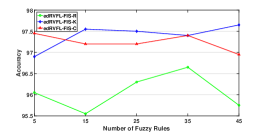
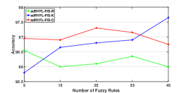
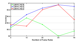
To examine the impact of fuzzy rules (clusters) on the performance of the proposed edRVFL-FIS models with varying sample sizes in the datasets, we conducted experiments by varying the number of fuzzy rules (). The resulting accuracy of the edRVFL-FIS models is investigated and visualized in Figure 2 w.r.t. the NDC datasets of size K, K, and M.
The noteworthy analyses are as follows:
-
1.
edRVFL-FIS-K: The accuracy of edRVFL-FIS-K shows a notable increase with the rise in fuzzy rules. Notably, tuning the fuzzy rules for edRVFL-FIS-K around or beyond tends to yield optimal performance.
-
2.
edRVFL-FIS-C: The optimal performance range for edRVFL-FIS-C is generally observed between fuzzy rules to . Fine-tuning in the neighborhood of tends to yield the highest accuracy.
-
3.
edRVFL-FIS-R: The performance pattern for edRVFL-FIS-R exhibits variations. For NDC-10K datasets, the optimal performance is at ; for NDC-100K, it peaks at ; for NDC-1M, the best performance is at . The mixed patterns in edRVFL-FIS-R highlight the dataset-dependent nature of optimal fuzzy rule selection.
Observations reveal discernible patterns in the performance of the proposed edRVFL-FIS-K and edRVFL-FIS-C models based on fuzzy rule variations. However, the performance varies across datasets and applications in accordance with the No Free Lunch Theorem [47]. Hence, a tailored approach to tuning fuzzy rules is recommended for optimizing the generalization performance of the proposed edRVFL-FIS models.
VI Conclusion and Future Work
We proposed the edRVFL-FIS model, a result of the seamless adaptation of FIS systems with edRVFL, meticulously crafted through a rigorous mathematical framework. The edRVFL-FIS model adeptly harnesses the synergy of deep learning, ensemble learning, and fuzzy logic, empowering the ensemble model to extract rich features effectively and enhance the learning process. The proposed edRVFL-FIS model integrates two significant feature components in each base model: unsupervised fuzzified features and supervised defuzzified features. Utilizing diverse clustering methods (R-means, K-means, Fuzzy C-means), it establishes fuzzy layer rules, resulting in three model variations (edRVFL-FIS-R, edRVFL-FIS-K, edRVFL-FIS-C) with unique fuzzified features. In addition, the ensemble structure utilizes diverse supervised defuzzified features for each base model, which improves the depth of feature extraction when making final predictions. The efficacy of the novel edRVFL-FIS models is showcased through extensive experimentation across multiple UCI datasets that cover a wide range of domains and sizes. Furthermore, we conducted experiments on big datasets using the NDC dataset. This experiment offers a comprehensive insight into the performance of the proposed edRVFL-FIS models across a diverse spectrum of data samples, ranging from to million. The empirical results demonstrate that the proposed edRVFL-FIS adaptably leverages fuzzification and defuzzification features to enhance generalization performance on large datasets. Additionally, we explored the influence of varying numbers of fuzzy rules (clusters) and hidden layers on the performance of the proposed edRVFL-FIS model. Moreover, we analyze the robustness of the proposed edRVFL-FIS models.
Within this study, we formulated an enhanced feature space incorporating both original and fuzzy features. Consequently, the presence of redundant features may contribute to increased computational complexity in the proposed models. This issue necessitates further discussion in the future. Moreover, we aim to advance our research by extending this work to regression problems and their application to biomedical domains such as brain age prediction. The source codes of the proposed models are available at https://github.com/mtanveer1/edRVFL-FIS.
Acknowledgment
This project is supported by the Indian government through grants from the Department of Science and Technology (DST) and the Ministry of Electronics and Information Technology (MeitY). The funding includes DST/NSM/R&D_HPC_Appl/2021/03.29 for the National Supercomputing Mission and MTR/2021/000787 for the Mathematical Research Impact-Centric Support (MATRICS) scheme. Furthermore, M. Sajid’s research fellowship is funded by the Council of Scientific and Industrial Research (CSIR), New Delhi, under the grant 09/1022(13847)/2022-EMR-I.
References
- Nandy et al. [2023] S. Nandy, M. Adhikari, V. Balasubramanian, V. G. Menon, X. Li, and M. Zakarya, “An intelligent heart disease prediction system based on swarm-artificial neural network,” Neural Computing and Applications, vol. 35, no. 20, pp. 14 723–14 737, 2023.
- Kurani et al. [2023] A. Kurani, P. Doshi, A. Vakharia, and M. Shah, “A comprehensive comparative study of artificial neural network (ann) and support vector machines (svm) on stock forecasting,” Annals of Data Science, vol. 10, no. 1, pp. 183–208, 2023.
- Sajid et al. [2023] M. Sajid, A. Malik, and M. Tanveer, “Intuitionistic fuzzy broad learning system: Enhancing robustness against noise and outliers,” arXiv preprint arXiv:2307.08713, 2023.
- Li et al. [2020] Z. Li, N. Kovachki, K. Azizzadenesheli, B. Liu, A. Stuart, K. Bhattacharya, and A. Anandkumar, “Multipole graph neural operator for parametric partial differential equations,” Advances in Neural Information Processing Systems, vol. 33, pp. 6755–6766, 2020.
- Gori and Tesi [1992] M. Gori and A. Tesi, “On the problem of local minima in backpropagation,” IEEE Transactions on Pattern Analysis and Machine Intelligence, vol. 14, pp. 76–86, 1992.
- Schmidt et al. [1992] W. F. Schmidt, M. A. Kraaijveld, and R. P. Duin, “Feed forward neural networks with random weights,” in International Conference on Pattern Recognition. IEEE Computer Society Press, 1992, pp. 1–1.
- Pao et al. [1994] Y.-H. Pao, G.-H. Park, and D. J. Sobajic, “Learning and generalization characteristics of the random vector functional-link net,” Neurocomputing, vol. 6, no. 2, pp. 163–180, 1994.
- Malik et al. [2023] A. K. Malik, R. Gao, M. A. Ganaie, M. Tanveer, and P. N. Suganthan, “Random vector functional link network: Recent developments, applications, and future directions,” Applied Soft Computing, vol. 143, p. 110377, 2023.
- Zhang and Suganthan [2016] L. Zhang and P. N. Suganthan, “A comprehensive evaluation of random vector functional link networks,” Information Sciences, vol. 367, pp. 1094–1105, 2016.
- Ganaie et al. [2024, doi:10.1109/TNNLS.2024.3353531] M. A. Ganaie, M. Sajid, A. K. Malik, and M. Tanveer, “Graph embedded intuitionistic fuzzy random vector functional link neural network for class imbalance learning,” IEEE Transactions on Neural Networks and Learning Systems, 2024, doi:10.1109/TNNLS.2024.3353531.
- Igelnik and Pao [1995] B. Igelnik and Y.-H. Pao, “Stochastic choice of basis functions in adaptive function approximation and the functional-link net,” IEEE Transactions on Neural Networks, vol. 6, no. 6, pp. 1320–1329, 1995.
- Hu et al. [2021] Y. Hu, B. Qu, J. Wang, J. Liang, Y. Wang, K. Yu, Y. Li, and K. Qiao, “Short-term load forecasting using multimodal evolutionary algorithm and random vector functional link network based ensemble learning,” Applied Energy, vol. 285, p. 116415, 2021.
- Qiu et al. [2018] X. Qiu, P. N. Suganthan, and G. A. Amaratunga, “Ensemble incremental learning random vector functional link network for short-term electric load forecasting,” Knowledge-Based Systems, vol. 145, pp. 182–196, 2018.
- Nayak et al. [2020] D. R. Nayak, R. Dash, B. Majhi, R. B. Pachori, and Y. Zhang, “A deep stacked random vector functional link network autoencoder for diagnosis of brain abnormalities and breast cancer,” Biomedical Signal Processing and Control, vol. 58, p. 101860, 2020.
- Shi et al. [2021] Q. Shi, R. Katuwal, P. N. Suganthan, and M. Tanveer, “Random vector functional link neural network based ensemble deep learning,” Pattern Recognition, vol. 117, p. 107978, 2021.
- Gao et al. [2023] R. Gao, R. Li, M. Hu, P. Suganthan, and K. F. Yuen, “Online dynamic ensemble deep random vector functional link neural network for forecasting,” Neural Networks, vol. 166, pp. 51–69, 2023.
- Li et al. [2023] R. Li, R. Gao, P. N. Suganthan, J. Cui, O. Sourina, and L. Wang, “A spectral-ensemble deep random vector functional link network for passive brain–computer interface,” Expert Systems with Applications, vol. 227, p. 120279, 2023.
- Sharma et al. [2023] R. Sharma, T. Goel, M. Tanveer, P. N. Suganthan, I. Razzak, and R. Murugan, “Conv-eRVFL: Convolutional neural network based ensemble rvfl classifier for alzheimer’s disease diagnosis,” IEEE Journal of Biomedical and Health Informatics, vol. 27, no. 10, pp. 4995–5003, 2023.
- Cheng et al. [2024] R. Cheng, R. Gao, and K. F. Yuen, “Ship order book forecasting by an ensemble deep parsimonious random vector functional link network,” Engineering Applications of Artificial Intelligence, vol. 133, p. 108139, 2024.
- He et al. [2023] J. He, X. Li, P. Liu, L. Wang, H. Zhou, J. Wang, and R. Tang, “Ensemble deep random vector functional link for self-supervised direction-of-arrival estimation,” Engineering Applications of Artificial Intelligence, vol. 120, p. 105831, 2023.
- Zadeh [1988] L. A. Zadeh, “Fuzzy logic,” Computer, vol. 21, no. 4, pp. 83–93, 1988.
- Sabri et al. [2013] N. Sabri, S. Aljunid, M. Salim, R. Badlishah, R. Kamaruddin, and M. Malek, “Fuzzy inference system: Short review and design,” Int. Rev. Autom. Control, vol. 6, no. 4, pp. 441–449, 2013.
- Xue et al. [2022] G. Xue, Q. Chang, J. Wang, K. Zhang, and N. R. Pal, “An adaptive neuro-fuzzy system with integrated feature selection and rule extraction for high-dimensional classification problems,” IEEE Transactions on Fuzzy Systems, 2022.
- Xie et al. [2023] R. Xie, C.-M. Vong, and S. Wang, “Doubly interpretable fuzzy apriori classifier by successive stacking and one-step wide calculation,” IEEE Transactions on Fuzzy Systems, 2023.
- Lee and Hu [2016] D. Lee and J. Hu, “Local model predictive control for T–S fuzzy systems,” IEEE Transactions on Cybernetics, vol. 47, no. 9, pp. 2556–2567, 2016.
- Wu et al. [2022] Y. Wu, H. Guo, H. Song, and R. Deng, “Fuzzy inference system application for oil-water flow patterns identification,” Energy, vol. 239, p. 122359, 2022.
- Vlasenko et al. [2019] A. Vlasenko, N. Vlasenko, O. Vynokurova, Y. Bodyanskiy, and D. Peleshko, “A novel ensemble neuro-fuzzy model for financial time series forecasting,” Data, vol. 4, no. 3, p. 126, 2019.
- Dosdoğru [2019] A. T. Dosdoğru, “Improving weather forecasting using de-noising with maximal overlap discrete wavelet transform and ga based neuro-fuzzy controller,” International Journal on Artificial Intelligence Tools, vol. 28, no. 03, p. 1950012, 2019.
- Zhang and Yang [2020] P.-B. Zhang and Z.-X. Yang, “A new learning paradigm for random vector functional-link network: RVFL+,” Neural Networks, vol. 122, pp. 94–105, 2020.
- Vuković et al. [2018] N. Vuković, M. Petrović, and Z. Miljković, “A comprehensive experimental evaluation of orthogonal polynomial expanded random vector functional link neural networks for regression,” Applied Soft Computing, vol. 70, pp. 1083–1096, 2018.
- Malik et al. [2022, https://doi.org/10.1109/TCSS.2022.3187461] A. K. Malik, M. A. Ganaie, M. Tanveer, and P. N. Suganthan, “Extended features based random vector functional link network for classification problem,” IEEE Transactions on Computational Social Systems, pp. 1–10, 2022, https://doi.org/10.1109/TCSS.2022.3187461.
- Takagi and Sugeno [1985] T. Takagi and M. Sugeno, “Fuzzy identification of systems and its applications to modeling and control,” IEEE Transactions on Systems, Man, and Cybernetics, no. 1, pp. 116–132, 1985.
- Talpur et al. [2023] N. Talpur, S. J. Abdulkadir, H. Alhussian, M. H. Hasan, N. Aziz, and A. Bamhdi, “Deep neuro-fuzzy system application trends, challenges, and future perspectives: A systematic survey,” Artificial Intelligence Review, vol. 56, no. 2, pp. 865–913, 2023.
- Ghosh and Dubey [2013] S. Ghosh and S. K. Dubey, “Comparative analysis of k-means and fuzzy c-means algorithms,” International Journal of Advanced Computer Science and Applications, vol. 4, no. 4, 2013.
- Havens et al. [2012] T. C. Havens, J. C. Bezdek, C. Leckie, L. O. Hall, and M. Palaniswami, “Fuzzy c-means algorithms for very large data,” IEEE Transactions on Fuzzy Systems, vol. 20, no. 6, pp. 1130–1146, 2012.
- Dua and Graff [2017] D. Dua and C. Graff, “UCI machine learning repository,” 2017.
- Musicant [1998] D. Musicant, “NDC: normally distributed clustered datasets,” Computer Sciences Department, University of Wisconsin, Madison, 1998.
- Huang et al. [2006] G.-B. Huang, Q.-Y. Zhu, and C.-K. Siew, “Extreme learning machine: theory and applications,” Neurocomputing, vol. 70, no. 1-3, pp. 489–501, 2006.
- Chen and Liu [2017] C. P. Chen and Z. Liu, “Broad learning system: An effective and efficient incremental learning system without the need for deep architecture,” IEEE Transactions on Neural Networks and Learning Systems, vol. 29, no. 1, pp. 10–24, 2017.
- Tang et al. [2015] J. Tang, C. Deng, and G.-B. Huang, “Extreme learning machine for multilayer perceptron,” IEEE Transactions on Neural Networks and Learning Systems, vol. 27, no. 4, pp. 809–821, 2015.
- Feng and Chen [2018] S. Feng and C. P. Chen, “Fuzzy broad learning system: A novel neuro-fuzzy model for regression and classification,” IEEE Transactions on Cybernetics, vol. 50, no. 2, pp. 414–424, 2018.
- Malik and Tanveer [2022, https://doi.org/10.1109/TCBB.2022.3202707] A. K. Malik and M. Tanveer, “Graph embedded ensemble deep randomized network for diagnosis of alzheimer’s disease,” IEEE/ACM Transactions on Computational Biology and Bioinformatics, pp. 1–13, 2022, https://doi.org/10.1109/TCBB.2022.3202707.
- Demšar [2006] J. Demšar, “Statistical comparisons of classifiers over multiple data sets,” The Journal of Machine Learning Research, vol. 7, pp. 1–30, 2006.
- Friedman [1937] M. Friedman, “The use of ranks to avoid the assumption of normality implicit in the analysis of variance,” Journal of the American Statistical Association, vol. 32, no. 200, pp. 675–701, 1937.
- Iman and Davenport [1980] R. L. Iman and J. M. Davenport, “Approximations of the critical region of the fbietkan statistic,” Communications in Statistics-Theory and Methods, vol. 9, no. 6, pp. 571–595, 1980.
- Kumar and Gopal [2009] M. A. Kumar and M. Gopal, “Least squares twin support vector machines for pattern classification,” Expert Systems with Applications, vol. 36, no. 4, pp. 7535–7543, 2009.
- Adam et al. [2019] S. P. Adam, S.-A. N. Alexandropoulos, P. M. Pardalos, and M. N. Vrahatis, “No free lunch theorem: A review,” Approximation and Optimization: Algorithms, Complexity and Applications, pp. 57–82, 2019.