On the Addams family of discrete frailty distributions for modelling multivariate case I interval-censored data
Abstract
Random effect models for time-to-event data, also known as frailty models, provide a conceptually appealing way of quantifying association between survival times and of representing heterogeneities resulting from factors which may be difficult or impossible to measure. In the literature, the random effect is usually assumed to have a continuous distribution. However, in some areas of application, discrete frailty distributions may be more appropriate. The present paper is about the implementation and interpretation of the Addams family of discrete frailty distributions. We propose methods of estimation for this family of densities in the context of shared frailty models for the hazard rates for case I interval-censored data. Our optimization framework allows for stratification of random effect distributions by covariates. We highlight interpretational advantages of the Addams family of discrete frailty distributions and the -point distribution as compared to other frailty distributions. A unique feature of the Addams family and the -point distribution is that the support of the frailty distribution depends on its parameters. This feature is best exploited by imposing a model on the distributional parameters, resulting in a model with non-homogeneous covariate effects that can be analysed using standard measures such as the hazard ratio. Our methods are illustrated with applications to multivariate case I interval-censored infection data.
Keywords Discrete distributions; Frailty; Heterogeneity; Infectious diseases; Multivariate survival data
1 Introduction
Multivariate time-to-event data are commonly encountered in the life sciences. An example is the time to occurrence of multiple non-lethal events within the same individual. In this setting, the individual can be thought of as forming a cluster in which event times are likely to be correlated. An alternative point of view is that there is heterogeneity across individuals (or clusters) due to characteristics that may be difficult or impossible to measure. Random effect (RE) models for time-to-event data, also known as frailty models, offer a conceptually appealing approach to quantify these associations within clusters and to model unobserved heterogeneity across individuals (or clusters) (Duchateau and Janssen,, 2008; Hougaard,, 2000; Wienke,, 2010).
While the majority of the existing literature assumes continuous frailty distributions, such as the gamma (), inverse Gaussian, or log-normal, for some applications discrete frailty distributions may be more appropriate. One such application is the study of infectious diseases transmitted via close contact, where unobserved heterogeneity with respect to becoming infected with pathogens of interest may be represented and analysed by latent risk groups.
This paper discusses the interpretation of discrete frailty models with parameter dependent support. We propose interpreting the discrete frailties as ordered latent risk categories. We extend this analysis by allowing the parameters of the discrete frailty distribution to depend on covariates. The ordered nature of discrete frailty facilitates comparing latent risk categories within or across different strata (as defined by covariate values) using hazard ratios, along with probabilities of belonging to specific risk categories. This approach facilitates the analysis of non-homogeneous populations or non-homogeneous covariate effects, which might lead to a deeper understanding of the problem under study.
In this context we discuss the “Addams” family () of discrete frailty distributions introduced by Farrington et al., (2012). This family is homogeneous in the sense that it consists of discrete distributions, except for the continuous distribution, which serves as a reference case of constant association within clusters over time. The discrete distributions within the are scaled variants of negative binomial, shifted negative binomial, binomial, and Poisson distributions. For this family, we investigate the hazard ratios conditional on risk group membership within or across different strata. Furthermore, we introduce estimation routines for the in the context of case I interval-censored data (Sun,, 2007). Our optimization framework allows for stratification of frailty distributions along covariates. We apply the to data from a serological survey of human papillomaviruses (Mollema et al.,, 2009; Scherpenisse et al.,, 2012).
The structure of the paper is as follows: Section 2 presents the time-invariant shared frailty model and reviews the literature on discrete frailty models, comparing the to other discrete frailty distributions. We further discuss the interpretation of discrete frailty models for which the support is parameter dependent. Section 3 examines the conditional time-to-event model resulting from the of distributions. Section 4 outlines the estimation framework and optimization algorithm. In Section 5, the is applied to multivariate serological survey data. Finally, Section 6 offers concluding remarks.
2 Discrete Frailty Models
Let refer to a cluster, , and let be the number of clusters observed. Each cluster contains units, and denotes the time-to-event random variable (RV) for the unit, , within the cluster. All indices are unique, such that and . The random vectors and are independent given the covariates and . Within a cluster, and are independent given the random and unobservable time-invariant cluster-specific frailty and covariates. The non-negative RV has density or probability mass function , where the index is relevant only if the distribution or its parameters depend on (a subset of) covariates denoted by . Technically, could include unit-specific covariates. However, as is shared within the cluster , will typically also be shared within the cluster , without containing covariates that differ across the units. For unit-specific covariates, correlated frailties (Hens et al.,, 2009) may be more appropriate, where the correlation parameter between the frailties of a cluster may depend on cluster-invariant covariates, while unit-specific frailty parameters may depend on unit-specific covariates. Given covariates, and are independent. We do not distinguish in language between the random and a realisation and refer to both as frailty or RE.
The conditional hazard rate, is assumed to be of the form
| (1) |
with cluster- and unit-specific covariate vector , and parameters , as well as unit-specific baseline hazard rate . Note that for brevity, the dependence of quantities, such as hazard rates or densities, on or is indicated by a superscript or subscript , respectively.
In much of the existing literature, is typically considered a continuous random variable, with common choices being the log-normal or distributions. Nonetheless, discrete frailty distributions have also been explored for both univariate and multivariate data. A prominent choice is the -point distribution (Palloni and Beltrán-Sánchez,, 2017; Bijwaard,, 2014; Begun et al.,, 2000; Gasperoni et al.,, 2020; Pickles and Crouchley,, 1994; Choi and Huang,, 2012; Choi et al.,, 2014; Troncoso-Ponce,, 2018), i.e. a frailty distribution with (ordered) support parameters and corresponding probability parameters for , and (Wienke,, 2010). Other choices are the binomial () (Ata and Özel,, 2013), negative binomial () (Ata and Özel,, 2013; Caroni et al.,, 2010), geometric (Caroni et al.,, 2010; Cancho et al.,, 2021; Choi and Huang,, 2012; Choi et al.,, 2014), Poisson () (Ata and Özel,, 2013; Caroni et al.,, 2010; Cancho et al., 2020b, ; Choi and Huang,, 2012; Choi et al.,, 2014), and the hyper-Poisson distributions (Mohseni et al.,, 2020; de Souza et al.,, 2017). The framework of the zero-inflated and zero-modified power series (ZMPS) distributions, where the probability of is modified by an additional parameter as compared to the discrete reference distribution, has been investigated by Cancho et al., (2018); Cancho et al., 2020a and Molina et al., (2021), respectively. In particular, the zero-inflated geometric, and logarithmic distributions and the zero-modified geometric and distributions are investigated. The Addams family (), as conceptualised by Farrington et al., (2012), includes (shifted and) scaled , as well as scaled and distributions, and the distribution as a continuous special case.
Modelling a whole family of distributions, such as the , is preferable to modelling a given (discrete) distribution, such as the , since the latter strategy typically severely limits the patterns of heterogeneity as measured by the relative frailty variance (, ) to either monotonically increasing or monotonically decreasing trajectories over time; for examples see Farrington et al., (2012) and Bardo and Unkel, (2023). It can be shown that the long-term trajectory of the RFV (or association, as measured by the cross-ratio function []) is determined with positive probability by the smallest value of the frailty distribution (). Specifically, if , and approach infinity as time approaches infinity. Conversely, if , the RFV approaches zero and the CRF approaches one. Therefore, the choice of a discrete frailty distribution has an enormous impact on the model, even if or is very small, and even more so if the model’s trajectory of RFV is monotone. The achieves greater flexibility in the trajectory of heterogeneity and association by incorporating discrete frailty distributions for which and frailty distributions for which , and is thus able to induce increasing and decreasing trajectories of the RFV (CRF). Thus, in the case of , the trajectory of the RFV can be informed by the data in the fitting process. This is a rare property among frailty distributions, and for the discrete distributions mentioned above it is only possible for the -point distribution and the ZMPS. However, in these cases the decision between a decreasing or increasing long-term trajectory lies on the edge of the parameter space (Bardo and Unkel,, 2023), which is not the case for the . As optimising on the edge of the parameter space is usually difficult, this is an advantage when using the . Note, however, that the -point distribution and the ZMPS are able to induce non-monotone trajectories of the RFV (CRF), which is not the case for the . We will discuss the and its special cases in Section 3.
From an interpretive point of view, the and -point distributions offer a unique perspective because the support is also subject to estimation. The support of other discrete frailty distributions is usually the natural number including zero (). Therefore, the interpretation of discrete frailty models often focuses on the cure rate, i.e. those who are not susceptible to the event of interest (see e.g. de Souza et al., (2017); Cancho et al., (2018); Cancho et al., 2020a ; Cancho et al., 2020b ; Mohseni et al., (2020); Cancho et al., (2021); Molina et al., (2021)). Subject-related interpretations are also common. Caroni et al., (2010) suggest interpreting discrete frailties as the unobservable number of flaws in a unit or exposure to damage on an unknown number of occasions. Similar interpretations can be found in Ata and Özel, (2013) for time-to-event models on earthquake data. Both studies consider discrete frailty distributions with support on . However, due to the latent nature of the frailty, such concrete interpretations are difficult because the hazard ratio (HR) of, say, two events versus one event would be fixed by the model structure at if the support is fixed at . However, if the true HR is less than two, the probability mass of frailty could be shifted to the right relative to the distribution of the number of hits. Consequently, a more abstract interpretation such as the “effective” number of harms would be more appropriate. The -point frailty distributions are often interpreted as representing sub-populations, such as unobservable carriers of certain disease genotypes (e.g., Pickles and Crouchley, (1994); Begun et al., (2000); Wienke, (2010); Bijwaard, (2014)). Palloni and Beltrán-Sánchez, (2017) interpret a delayed binary frailty as the effect of adverse early life conditions on adult mortality. Using the -point distribution, where is also subject to estimation, Gasperoni et al., (2020) interpret the discrete frailties as (an unknown number of) latent sub-populations. They suggest calculating HRs between these sub-populations, which is interpretable as the support being subject to estimation.
In the present paper, we endorse the interpretation of discrete frailties as latent sub-populations and expand upon it. Note that we focus on discrete frailty distributions for which the support is parameter dependent, which is mainly the case for the -point distribution and, although more restricted, the , as will be seen in Section 3. Let , with and , represent the support of discrete RV , where the distribution parameters might depend on . We define that constitutes a stratum of the population. We also consider as the conditional hazard-determining value for an individual in the risk category (RC) within the stratum which is defined by .
For discrete frailty distributions for which the support depends on parameters, the within-stratum hazard ratio, , might be analysed. The compares the hazard of the and RC of stratum . This is in line with Gasperoni et al., (2020), except for the presence of different strata for the distribution of the frailty, i.e. the might differ for and . Moreover, due to the presence of different strata for the frailty distribution, an across-stratum analysis can be conducted by computing the across-stratum hazard ratio, , for , and equality in the remaining covariates. If the support between stratum and is very different, it might be more desirable to analyse for all for which or the closest quantiles of if no such exists. In order to put the analysis of the and into context, they should always be accompanied by reporting the distribution of the RCs. This allows for a separate but accompanying analysis of the distribution of individual heterogeneity via the distribution of RCs and the magnitude related impact of the RCs on the hazard rates.
The approach of imposing a model on the distribution parameters of the frailty has some similarity to generalized additive models for location, scale, and shape parameters for the population time-to-event distribution, i.e. for the time-to-event distribution with the frailty marginalized out. However, modelling the determinants of the randomness of hazard rates via covariates might be more intuitive, as the hazard rates are usually the standard approach for modelling time-to-event data. This approach is not new per se. It can be found, for example, in Aalen et al., (2008) and is also quite common in the field of discrete frailty modelling (Choi and Huang,, 2012; Choi et al.,, 2014; Molina et al.,, 2021; Cancho et al.,, 2018; Cancho et al., 2020a, ), and random slopes could also be interpreted in this way. What is new, however, is the type of analysis with within-stratum and across-stratum hazard ratios. Note that this type of analysis has no counterpart for continuous frailty distributions, as there is no RC. Nor does such an analysis make sense for discrete frailty models where the support of the frailty distribution is set by assumption, e.g. to , as this would fix the and by assumption. Therefore, an analysis via the and is unique to discrete frailty models, where the support of the frailty distribution varies with (a subset of) distribution parameters that may depend on stratum membership. In this case, the data inform the support of the frailty distribution by likelihood criteria making it suitable to represent latent RCs. This allows the analysis of non-homogeneous covariate effects using common measures such as HRs as described above and probabilities of belonging to a particular RC. This might in particular be helpful in communicating the results of heterogeneous (covariate) effects to an audience outside of statistics such as medical doctors.
3 The Addams Family of Discrete Frailty Distributions
Let denote the cumulative baseline hazard rate . Moreover, . We further ignore that the parameters of the frailty distribution may depend on in the first part of this section and come back to this issue in the latter part of this section.
The RFV that induces the equals , with , and . As shown in Farrington et al., (2012), the Laplace transform of the equals
| (2) |
Note that may be set to one for identification purposes. Hence, the is a two parameter distribution. We will keep in the notation, however, as we will explicitly model the parameter via , where is an additional set of parameters which is usually interpreted as proportional hazard factor on the baseline hazard rate.
| Parameters | Distribution Parameters | Support | |
|---|---|---|---|
| (number of successes), | |||
| (success probability) | |||
| (shape), (rate) | |||
| (rate) | |||
| (number of successes), | |||
| (success probability) | |||
| (number of trials), | |||
| (success probability) |
The Laplace transform uniquely determines the distribution of , as shown in Table 1 (Farrington et al.,, 2012). The consists of different scaled and possibly shifted discrete distributions. The scaling parameter of the corresponding discrete distributions is equal to , and the parameter selects one of the distributions of the . If , the scaled and shifted negative binomial () is chosen, where the support is shifted to the right by the parameter , resulting in a model without a latent non-susceptible sub-population. If , a frailty distribution is chosen that includes a non-susceptible latent sub-population. For , the non-shifted scaled negative binomial () and for the scaled Poisson () distribution is selected. In the case of , the frailty distribution is scaled binomial (), resulting in a model with an upper bound of the frailty that limits the maximum deviation of RC-conditioned survival curves between the susceptible latent sub-populations and a finite number of RCs including a non-susceptible group. Note that for the case , has to be an integer in order for to be a valid Laplace transform (Farrington et al.,, 2012). The continuous exception in the is the distribution, which results from .
The parameter plays a unique role in the context of discrete shared frailty modelling. For discrete shared frailty models the RFV (CRF) either approaches zero (one) or infinity (Bardo and Unkel,, 2023). Therefore, it is desirable to have a continuous exception within a family of discrete shared frailty distributions for which the RFV (CRF) does not approach zero (one) or infinity with time approaching infinity. Within the context of the this is the which arises for . In that case the RFV (CRF) is constant, a shape that is impossible for a discrete shared frailty model to generate. The nested structure might be utilized to test for a constant RFV (CRF) within the .
Moreover, the can choose between a monotonically decreasing or increasing trajectory of the RFV (CRF) through the sign of . This is unprecedented in the context of discrete shared frailty models. Though the ZMPS distribution is able to create decreasing trajectories of the RFV (CRF), this involves the edge of the parameter space for its deflation/inflation parameter. The opposite is true for the -point distribution: its RFV (CRF) approaches zero (one) in the long run unless is equal to zero, which again involves the edge of the parameter space. For the , the parameter chooses between a decreasing or increasing RFV (CRF) by determining the support of the discrete distribution without involving the edge of parameter space. If , and a cure fraction exists. This induces an increasing trajectory of the RFV (CRF). If instead, and no cure fraction exists. This induces a decreasing trajectory of the RFV (CRF); see Bardo and Unkel, (2023) for a discussion of the shape of the RFV (CRF) for discrete frailty models.
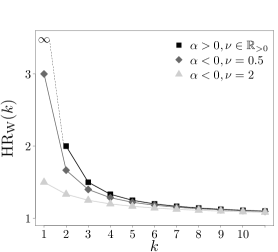
The feature of the support being dependent on the distribution parameters offers the possibility of a meaningful interpretation of the . Figure 11(a) shows examples of the for and . If , and for . Note that there may be an upper bound on the RCs if is chosen. In this case, the upper bound of the frailty as well as the number of RCs chosen through the fitting procedure may be the main component of the analysis, e.g. by comparing the RC-related survival curve of the upper bound versus another RC. If , which approaches for large . So there is reasonable flexibility for the first few within-stratum HRs and the focus may be on , where the model is more flexible than for later RCs. This is less flexible than the -point distribution is, provided that is large enough, which may even show a non-monotone trajectory of the . However, modelling the -point distribution with a large is difficult given that this involves parameters for a latent distribution, especially if the cluster size is small. On the contrary, within the one is remunerated with (except for the case) which can be important for extreme observations where events occur very early in the lifespan. However, the parametric constraints of the on the trajectory of should always be taken in consideration and challenged by the -point distribution whenever possible.
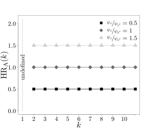
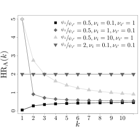
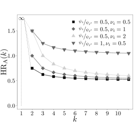
This analysis can be extended to the across-stratum HR, , if there is a model for the distribution of individual heterogeneity within the . For that purpose, we allow the parameters to depend on a stratum-specifying set of covariates , which determine the parameters of individual heterogeneity , with each parameter in the vectors being an element of . For the sake of brevity, we denote and by and , respectively. Figure 1 shows the for varying scenarios of and . For (Figure 11(b)), the for all and is undefined for . However, for (Figure 11(c)), the , which approaches a constant ratio for large . Note that the might be greater or less than one for all , but can also cross the threshold of one with increasing . If is for example an experimental treatment indicator (in a univariate context), the represents a heterogeneous treatment effect which might identify sub-groups within the population for which the treatment is harmful. For (Figure 11(d)), , as for stratum there is a latent sub-population that is not susceptible to the event of interest, whereas for stratum all latent sub-populations are susceptible. For and . Another scenario, not explicitly shown in Figure 1(b) and 1(d), is that one or both strata ( and ) might have (different) upper bounds of frailty in the case. In such a case, the stratum with the larger upper bound (which could still be ), say , could be considered more vulnerable, since that stratum has a higher proportion of individuals who are expected to experience the event very early, namely those with a frailty value greater than .
Note that the parameters in the formulæ of and (and hence the parameters as specified in the legends of Figure 1) do not uniquely identify the parameters of the frailty distribution, i.e. for a given trajectory of there is an infinite set of or and , respectively, that induce the same trajectory but with a different distributions of the RCs which did not need to be specified for Figure 1. This shows that the analysis of the frailty model has always two branches. The first branch is the analysis of HRs, which indicate the meaning of being in a particular latent RC (in a particular stratum) relative to another latent RC or to another observable stratum in the same latent RC. On the one hand, can help to assess the importance of individual heterogeneity, e.g. if is large, then latent RC membership has a large effect on expected survival. On the other hand, comparing across strata or analysing the gives an account of random covariate effects where, e.g., covariates with a beneficial effect on survival or covariates with partly beneficial, partly detrimental effects might be detected. The second branch of the analysis is the distribution of RCs across strata, which may indicate differences in the distribution of risk-taking behaviour and predisposition across strata, e.g. by indicating a stratum with a heavier tail of vulnerable RCs. Taken together, the analysis of HRs and the distribution of RCs can provide thorough analytical explanations in terms of selection and random covariate effects that can help to explain the trajectories of population survival curves (where the RCs are marginalised out), i.e. explanations for why the survival curves of two strata come closer or even cross over time.
4 Estimation
In this section, all time-dependent quantities are evaluated at the monitored (censored or uncensored) event times of the individuals. We delete the argument from the expression and indicate the corresponding quantity with a subscript, e.g. . Furthermore, let , where denotes the power set. Then, and . Note that we define and .
We develop estimation routines for case I interval-censored data. In the case of case I interval-censored data it is only known whether the event occurred during follow-up or not but the exact event time is unknown. For multivariate cases () it is easier to understand the likelihood if one starts by exploiting the conditional independence assumption of and , given :
| (3) |
where is the observational unit and target-specific event indicator (equal to one if the event occurred during the follow-up, zero otherwise), and is the set of targets on which the observational unit had an event. The vector contains all parameters of the baseline hazard rates, , and .
Quasi-Newton optimization routines were applied for optimizing the corresponding log-likelihood based on (3). We choose BFGS as the standard method, as implemented in R version 4.2.2 (R Core Team,, 2022). Standard errors (SE) are obtained via the Hessian of the log-likelihood, which is approximated by Richardson extrapolation as implemented by Gilbert and Varadhan, (2019). The delta method was applied where necessary to obtain SE: confidence intervals (CIs) are based on or transformations if the parameter of interest is greater than zero or between zero and one respectively, and are then transformed back to the scale of interest.
We provide algorithms that are able to fit univariate and multivariate frailty models for case I interval-censored data. The frailty distributions can be stratified by a (multi-level) factor. The frailty distribution might either be or from the power variance family (both parameters can be estimated). The baseline hazard can be chosen to be piecewise-constant or the parametric generalized gamma distribution (Cox et al.,, 2007) or one of its special cases, respectively. Covariates can be added in proportional hazards manner. Overdispersion parameters might be added by means of the Dirichlet compound multinomial distribution. Implementations are available on GitHub (https://github.com/time-to-MaBo/Addamsfamily/).
5 Applications
We illustrate the in the context of multivariate case I interval-censored data on the human papillomavirus (HPV), obtained from a serological survey in the Netherlands (PIENTER-2); see Mollema et al., (2009) for details on PIENTER-2 and Scherpenisse et al., (2012) for an investigation of the respective HPV dataset. The data were collected in the years 2006 and 2007 and cover people aged 0 to 79. Participants were asked to complete a questionnaire and to provide a blood sample (Mollema et al.,, 2009). By means of the blood samples, the level of antibodies regarding the high-risk HPV types 16, 18, 31, 33, 45, 52, and 58 were determined in order to detect past infections. Therefore, at the time of observation, it is only known whether the study participants have had an infection in the past or not, but it is never known exactly when the potential infection occurred, resulting in case I interval-censored data, also known as current status data (Sun,, 2007). Note that at the time of data collection the Dutch national immunization programme did not include a vaccine against HPV.
We analysed the nationwide sample including oversampled migrants and applied weighting factors to make the sample representative for the Dutch population. We excluded individuals in their first year of life from the analysis, as maternal antibodies could be transmitted to the infant transplacentally or through breastfeeding (Rintala et al.,, 2005). This left us with a sample size of individuals aged 2 to 80. The weighted proportion of females in the dataset is % (unweighted: %).
The observed time is the individuals’ age at the date of serological monitoring. The event indicator means that individual is seropositive with respect to pathogen , , and seronegative and still susceptible if . Seroprevalence is interpreted as a proxy for past infections. Note, however, that there is a time-lag between the infection and the time of seroconversion, as well as a difference in the number of individuals who were infected with HPV and those who seroconverted: in previous studies, antibodies could not be detected for about 20-50% of females who were carriers of HPV DNA. However, antibody responses are relatively stable over time and hence, the study of the population’s seroprevalence might yield important insights; see Scherpenisse et al., (2012) for a discussion.
We consider the following models for the individual hazard rates, , , where the target-specific baseline hazard is either sex-stratified (sex-stratified baseline hazard model), or non-stratified (non-stratified baseline hazard model). The purpose of stratifying baseline hazards by sex is twofold. The first is to investigate whether it is justified to estimate baseline hazards jointly for both sexes, and the second is to investigate whether a potential difference in the distribution is better explained by stratified baseline hazards than by different distributions of individual heterogeneity. In any case the target (and potentially sex) specific hazard rate is piecewise constant with a unique parameter within the intervals , , , , , , , . The frailty is either sex-stratified, i.e. (sex-stratified RE model), or non-stratified, i.e. (non-stratified RE model). Note that in both cases , except for the stratified-hazard model where is also set to one for the sake of identifiability. The stratified RE model might be better able to reflect differing patterns in individual heterogeneity due to biological and environmental predisposition as well as a different distribution of risk-related behaviour across males and females. We combine the stratification status of the baseline hazard with the stratification status of the RE.
An HPV infection can be transmitted via skin-to-skin contact, often - though not exclusively (see, e.g., Syrjänen, (2010), Rintala et al., (2005) or Meyers et al., (2014)) - via sexual intercourse (Gavillon et al.,, 2010). Therefore, individual – and typically unobserved – behaviour is an important determinant of an individual’s risk of contracting HPV. Frailty models have been used previously to incorporate unobservable individual heterogeneity in the transmission of infectious diseases (see, e.g., Unkel et al., (2014) or Hens et al., (2009)). Moreover, we suspect that there may be distinct jumps in the individual hazard rates due to differences in individual behaviour that are relevant for transmission, e.g. comparing individuals who have no sex at all to individuals who have (see, e.g., Richardson et al., (2000), Burchell et al., (2006)), or whether the individuals use condoms or not (see, for example, Lam et al., (2014) or Nielson et al., (2010)). More formally, non-Gaussian and discrete omitted covariates may be the most important drivers of individual heterogeneity, and thus a discrete frailty model may be particularly appropriate here.
We start with a bivariate analysis including HPV16 and HPV18. An extension to higher variate data with data on seven types of HPV follows.
5.1 Bivariate Data Analysis
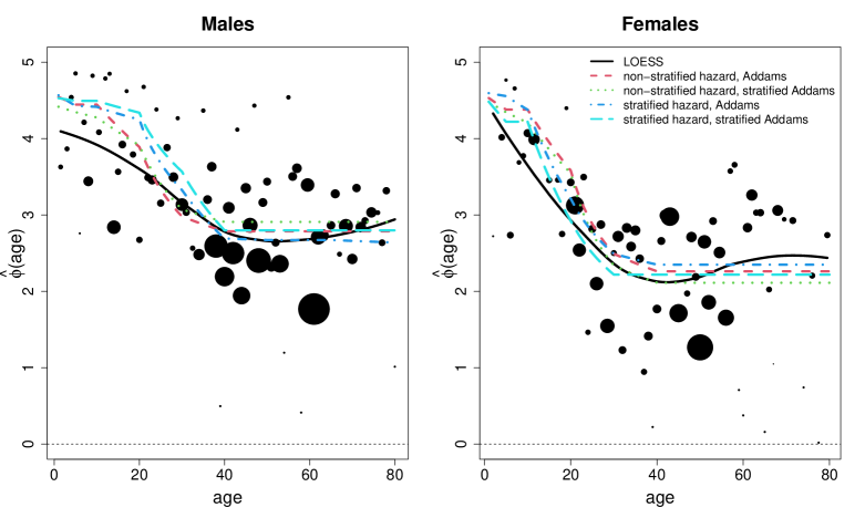
We begin by exploiting the nested structure of the models for model selection. The stratification of the RE is statistically significant on conventional levels by means of a likelihood ratio test (LRT) no matter the stratification status of the baseline hazard. The null-hypothesis is : vs. . Note that the expectation parameter is not included in the hypothesis. In the case of non-stratified baseline hazards the LRT test statistic equals 29.700 on 2 degrees of freedom (p-value 0). In the case of sex-stratified baseline hazards the LRT test statistic equals 30.822 on 2 degrees of freedom (p-value 0). Better performance of stratified RE models is also suggested by the -plot which can be seen in Figure 2(a). The measure is an association measure for bivariate current status data introduced by Unkel and Farrington, (2012), indicates positive and negative association. Additionally, tracks with a time-lag. It can be observed that the association between HPV16 and HPV18 is higher for females early in life, but declines more strongly than for males. This is likely to be the reason for the success of stratified RE models here as those models are able to choose a distinct intercept and slope of the RFV across the sexes. We choose the sex-stratified RE model for further analysis.
In terms of AIC, the non-stratified baseline hazard model , performs better than sex-stratified-baseline hazard model (9647 vs. 9656). Thus, we choose the non-stratified baseline hazard, stratified RE model for further analysis.
A LRT for a constant RFV (CRF), i.e. vs. for males and females, yields a test-statistic of 93.514 on 2 degrees of freedom (p-value ). Hence, the hypothesis on a constant RFV (CRF) can also be rejected. A constant pattern of the RFV is also not suggested by Figure 2(a), where it can be observed that association is constantly falling up to the age of around . Considering all tests and pairwise AIC comparisons we choose the non-stratified baseline hazard, stratified model for final analysis.
| male | female | |
|---|---|---|
| \hdashline | ||
| RC | males | females | males | females | ||
|---|---|---|---|---|---|---|
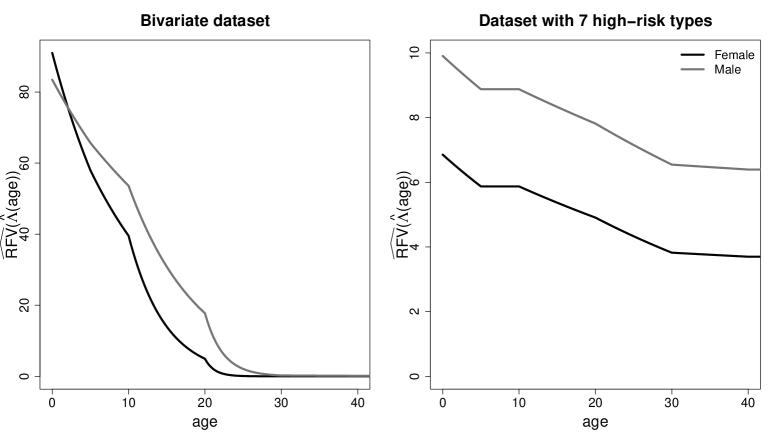
The RFV parameter estimates for the stratified RE, non-stratified baseline hazard models can be seen in Table 2. The estimated RFV (CRF) is decreasing for both sexes. The estimated RFV parameters indicate higher heterogeneity across clusters or association within a cluster for females early on, as indicated by the intercept of the RFV (). However, the descent is more strongly for females () and consequently it is estimated that heterogeneity/association is stronger for males from the 4 year of life onwards; see left-hand panel of Figure 2(b). These results are also supported by the non-parametric estimates of in Figure 2(a).
The estimated distribution corresponds to a for males and females. The mean parameter and is highly insignificant as indicated by the -CI. The resulting distribution parameters can also be found in Table 2. The estimated mean indicates lower expected frailty (and therefore lower population hazard) for females initially. However, the mean parameter has to be interpreted in the context of its distribution. Let . The limit of the conditional expectation of the frailty is . With the estimates from Table 2, 0.01 0.006 follows and the initial order of the expectations is reversed. In this example, this leads to the estimated population seroprevalence being higher for males early in life but from 12 years of life onwards, females start to catch up and finally cross the curve of males at 25 years of life (not shown). We will discuss the reason for the switching order of , and that finally leads to crossing seroprevalence curves by analysing the distribution of the frailties in the paragraphs below.
Table 3 shows an excerpt of the distribution of the RCs. We interpret the distribution of the RCs as the distribution of stratum-relative risk-related behaviour and predisposition. The bulk of the population is estimated to be in the lowest RC, though there is more probability to the right of the lowest RC for males. The ratio of the cumulative probabilities between females and males is always above one, also indicating a more heavy tail for males. The heavier tale of the distribution of latent RCs for males is the reason for .
The numerical value of the frailties then assigns a magnitude related interpretation to the distinct RCs. The estimated support shows that females have a higher category-related hazard in each RC (see the last column Table 3). Across strata, given the RC, the conditional or RC-related HR, , is 1.684 in the important first category. In this case, the approaches its limit (with respect to ), 1.883, fast due to small values of . Higher RC-related hazard for females is the reason for surpassing with time progressing: the individuals belonging to the tale of the distribution of the RCs start to seroconvert early. This selection effect is more pronounced for males due to the heavier tale of the distribution of RCs. Due to extreme individuals within the male population seroconverting more quickly, the higher RC-related hazard for females causes from 12 years of life onwards.
Within stratum, for females and for males, i.e. being in the second instead of the lowest RC is estimated to be more hazardous for females than for males even from a relative perspective. The then approaches its limit immediately because is small for males and females.
Differences in unobserved heterogeneity across the sexes are reflected by the support and the distribution of the RCs. Given that HPV is a sexually transmitted disease, the membership to a certain RC is partly governed by stratum-relative (sexual) behaviour in that sense, that having, for example, a higher number of sexual partners than some stratum reference should put one in a higher RC than the reference individual. It is tempting to interpret the difference in magnitude of a given RC on the conditional hazard rate across the sexes. For the human immunodeficiency viruses, for example, it is known that male to female transmission is more likely than female to male transmission (see Nicolosi et al., (1994) or European Study Group on Heterosexual Transmission of HIV, (1992)). Assuming that each RC comprises the same set of sexual behaviour across the sexes, for all , could also hint on a higher susceptibility of females with respect to an infection with HPV16 and HPV18 per relevant contact. However, the RCs are anchored in the stratum and do not necessarily imply the same behaviour across the sexes. Hence, this interpretation is highly speculative and assumption based.
5.2 Higher Variate Analysis
When including all seven high-risk types of HPV for which we have data, the direction of interpretation is largely similar to that of the bivariate case, and mainly the magnitude changes. The estimated RFV parameters are , , , . The heterogeneity/association is less extreme than in the bivariate case early in life. However, the association remains at larger levels compared to the bivariate case, as shown in Figure 2(b), indicating that association remains high throughout life. It can also be seen that the RFV (CRF) of females is always below that of males, indicating greater heterogeneity due to individual factors for males throughout the entire time period. As the level of association differs strongly between the bivariate case above and the higher variate case with seven high-risk HPV types, a shared frailty model might be seen as inadequate to capture the patterns of association between the various types of HPV. Therefore, a correlated frailty model may be more appropriate. The shared frailty model might be chosen for its simplicity, however, if the specific types of HPV are less relevant to the research question but, for example, the prognostic factor of one “anonymous” high-risk type on another “anonymous” high-risk type is investigated.
The (initial) expectation of the frailty is virtually identical for males and females; . In the higher variate case the distribution of the RCs is not as much focused on the lower categories. The tail is again more heavy for males (not shown). The for all again indicates higher RC-related hazard for females. The is less extreme in the higher variate case than in the bivariate case: for females and for males. Note that the order of for males and females changes when comparing this to the bivariate scenario.
6 Conclusion
In this paper, we discuss the Addams family of discrete frailty distributions, which has been conceptualised by Farrington et al., (2012) for modelling individual heterogeneity in time-to-event models. We further examine the properties of the conditional time-to-event model induced by the Addams family and develop estimation routines for multivariate case I interval-censored data.
For discrete frailty distributions, the RFV (CRF) approaches either infinity or zero (one) over the course of time, where the distinction is made by the minimum of the support of the frailty being zero or greater than zero respectively. Few discrete frailty distributions are able to manipulate the support via its parameters to choose the long-term behaviour of the two functions accordingly, but this typically involves the edge of the parameter space; see Bardo and Unkel, (2023) for a discussion. For the Addams family of discrete frailty distributions, the minimum of the support can either be zero, resulting in a cure rate model, or greater than zero without involving the edge of the parameter space. Consequently, the RFV (CRF) is either monotonically increasing or monotonically decreasing, again without involving the edge of the parameter space. Through the introduction of a scaling parameter, the Addams family is also able to increase or flatten the slope of the RFV (CRF) and might even approach a constant by approaching its continuous exception, a shape that is impossible for discrete shared frailty model to generate. This makes the Addams family a useful general-purpose modelling approach.
A unique feature of the Addams family is that the support of the discrete frailty distribution varies with its parameters and is hence subject to estimation. We suggest interpreting the support as ordered latent risk categories. This feature allows for a unique analysis of the latent model through calculating hazard ratios across different latent risk categories. We call this the within-stratum hazard ratio. If a model is imposed on the distribution parameters of the Addams family, this analysis can be enriched by the across-stratum hazard ratio, i.e. the hazard ratio of a given latent risk category for different strata that are defined by covariates. This type of analysis could also be performed with the discrete -point distribution. However, there is no counterpart to this analysis for continuous frailty distributions, or for discrete frailty distributions for which the support is fixed. Thus, the Addams family and the -point distribution offer the possibility to analyse the latent model, which may include heterogeneous covariate effects, more thoroughly.
The analysis of the latent model via the within-stratum hazard ratio might help to understand the importance of individual heterogeneity. In that sense, individual heterogeneity might be regarded as important if the within-stratum hazard ratios are large and vice versa. The analysis of the across-stratum hazard ratio may reveal structural differences in individual heterogeneity across covariates, prompting a discussion of the reasons for this. Furthermore, it is an advantage that this analysis can be carried out via the analysis of time-invariant hazard ratios, which is arguably the most common way to analyse data in time-to-event analysis. Hence, we think the interpretation of the within-stratum and across-stratum hazard ratios is a particular suitable way to communicate with an audience outside of statistics. Due to the discrete latent random variables, the analysis can further be enriched with probabilities of belonging to a certain risk category (conditional on survival up to ) and the corresponding differences across strata, which should be straightforward to communicate.
We applied the Addams family to multivariate case I interval-censored infection data and allowed the distribution of individual heterogeneity to differ for males and females. Males are found to have a higher probability for more hazardous categories, possibly reflecting a more cautious behaviour in the female population compared to males. However, the estimated hazard in each risk category is higher for females than for males, which might reflect a higher biological burden with respect to the susceptibility of HPV. There was no evidence for the existence of a non-susceptible sub-group, neither in the bivariate data set, including HPV 16 and HPV 18, nor in the data set containing seven high-risk types of HPV.
Competing interests
No competing interest is declared.
Acknowledgments
We are grateful to Fiona van der Klis and Liesbeth Mollema from the Dutch National Institute for Public Health and the Environment (RIVM), for giving us permission to use the data from the second PIENTER study. The authors also thank the anonymous reviewers for their valuable suggestions. This work was supported by the Deutsche Forschungsgemeinschaft (DFG; German Research Foundation) [grant number UN 400/2-1].
References
- Aalen et al., (2008) Aalen, O. O., Borgan, Ø., and Gjessing, H. K. (2008). Event History Analysis: A Process Point of View. Statistics for Biology and Health. Springer, Dordrecht.
- Ata and Özel, (2013) Ata, N. and Özel, G. (2013). Survival functions for the frailty models based on the discrete compound poisson process. Journal of Statistical Computation and Simulation, 83(11):2105–2116.
- Bardo and Unkel, (2023) Bardo, M. and Unkel, S. (2023). The shape of the relative frailty variance induced by discrete random effect distributions in univariate and multivariate survival models. https://arxiv.org/pdf/2303.04915, pages 1–25.
- Begun et al., (2000) Begun, A. Z., Iachine, I. A., and Yashin, A. I. (2000). Genetic nature of individual frailty: comparison of two approaches. Twin Research and Human Genetics, 3(1):51–57.
- Bijwaard, (2014) Bijwaard, G. (2014). Multistate event history analysis with frailty. Demographic Research, 30:1591–1620.
- Burchell et al., (2006) Burchell, A. N., Winer, R. L., de Sanjosé, S., and Franco, E. L. (2006). Chapter 6: Epidemiology and transmission dynamics of genital hpv infection. Vaccine, 24 Suppl 3:S3/52–61.
- Cancho et al., (2021) Cancho, V. G., Barriga, G., Leão, J., and Saulo, H. (2021). Survival model induced by discrete frailty for modeling of lifetime data with long-term survivors and change-point. Communications in Statistics - Theory and Methods, 50(5):1161–1172.
- (8) Cancho, V. G., Macera, M. A. C., Suzuki, A. K., Louzada, F., and Zavaleta, K. E. C. (2020a). A new long-term survival model with dispersion induced by discrete frailty. Lifetime Data Analysis, 26(2):221–244.
- (9) Cancho, V. G., Suzuki, A. K., Barriga, G. D. C., and do Espirito Santo, Ana P. J. (2020b). A multivariate survival model induced by discrete frailty. Communications in Statistics - Simulation and Computation, pages 1–19.
- Cancho et al., (2018) Cancho, V. G., Zavaleta, K. E. C., Macera, M. A. C., Suzuki, A. K., and Louzada, F. (2018). A bayesian cure rate model with dispersion induced by discrete frailty. Communications for Statistical Applications and Methods, 25(5):471–488.
- Caroni et al., (2010) Caroni, C., Crowder, M., and Kimber, A. (2010). Proportional hazards models with discrete frailty. Lifetime Data Analysis, 16(3):374–384.
- Choi and Huang, (2012) Choi, S. and Huang, X. (2012). A general class of semiparametric transformation frailty models for nonproportional hazards survival data. Biometrics, 68(4):1126–1135.
- Choi et al., (2014) Choi, S., Huang, X., and Chen, Y.-H. (2014). A class of semiparametric transformation models for survival data with a cured proportion. Lifetime Data Analysis, 20(3):369–386.
- Cox et al., (2007) Cox, C., Chu, H., Schneider, M. F., and Muñoz, A. (2007). Parametric survival analysis and taxonomy of hazard functions for the generalized gamma distribution. Statistics in Medicine, 26(23):4352–4374.
- de Souza et al., (2017) de Souza, D., Cancho, V. G., Rodrigues, J., and Balakrishnan, N. (2017). Bayesian cure rate models induced by frailty in survival analysis. Statistical Methods in Medical Research, 26(5):2011–2028.
- Duchateau and Janssen, (2008) Duchateau, L. and Janssen, P. (2008). The Frailty Model. Springer, Dordrecht.
- European Study Group on Heterosexual Transmission of HIV, (1992) European Study Group on Heterosexual Transmission of HIV (1992). Comparison of female to male and male to female transmission of hiv in 563 stable couples. european study group on heterosexual transmission of hiv. BMJ (Clinical research ed.), 304(6830):809–813.
- Farrington et al., (2012) Farrington, C. P., Unkel, S., and Anaya-Izquierdo, K. (2012). The relative frailty variance and shared frailty models. Journal of the Royal Statistical Society. Series B (Statistical Methodology), 74(4):673–696.
- Gasperoni et al., (2020) Gasperoni, F., Ieva, F., Paganoni, A. M., Jackson, C. H., and Sharples, L. (2020). Non-parametric frailty cox models for hierarchical time-to-event data. Biostatistics (Oxford, England), 21(3):531–544.
- Gavillon et al., (2010) Gavillon, N., Vervaet, H., Derniaux, E., Terrosi, P., Graesslin, O., and Quereux, C. (2010). Papillomavirus humain (hpv) : comment ai-je attrapé ça ? Gynecologie, obstetrique & fertilite, 38(3):199–204.
- Gilbert and Varadhan, (2019) Gilbert, P. and Varadhan, R. (2019). numderiv: Accurate numerical derivatives. https://cran.r-project.org/web/packages/numDeriv/.
- Hens et al., (2009) Hens, N., Wienke, A., Aerts, M., and Molenberghs, G. (2009). The correlated and shared gamma frailty model for bivariate current status data: an illustration for cross-sectional serological data. Statistics in Medicine, 28(22):2785–2800.
- Hougaard, (2000) Hougaard, P. (2000). Analysis of Multivariate Survival Data. Springer, New York.
- Lam et al., (2014) Lam, J. U. H., Rebolj, M., Dugué, P.-A., Bonde, J., von Euler-Chelpin, M., and Lynge, E. (2014). Condom use in prevention of human papillomavirus infections and cervical neoplasia: systematic review of longitudinal studies. Journal of Medical Screening, 21(1):38–50.
- Meyers et al., (2014) Meyers, J., Ryndock, E., Conway, M. J., Meyers, C., and Robison, R. (2014). Susceptibility of high-risk human papillomavirus type 16 to clinical disinfectants. The Journal of Antimicrobial Chemotherapy, 69(6):1546–1550.
- Mohseni et al., (2020) Mohseni, N., Maboudi, A. A. K., Baghestani, A., and Saeedi, A. (2020). A cure rate model with discrete frailty on hodgkin lymphoma patients after diagnosis. Archives of Advances in Biosciences, 11(4):15–22.
- Molina et al., (2021) Molina, K. C., Calsavara, V. F., Tomazella, V. D., and Milani, E. A. (2021). Survival models induced by zero-modified power series discrete frailty: application with a melanoma data set. Statistical Methods in Medical Research, 30(8):1874–1889.
- Mollema et al., (2009) Mollema, L., de Melker, H. E., Hahne, S. J., van Weert, J. W., Berbers, G. A., and van der Klis, F. R. (2009). PIENTER 2-project: second research project on the protection against infectious diseases offered by the national immunization programme in the Netherlands (Report 230421001/2009). Rijksinstituut voor Volksgezondheid en Milieu RIVM.
- Nicolosi et al., (1994) Nicolosi, A., Maria Léa Corrêa Leite, Musicco, M., Arici, C., Gavazzeni, G., and Lazzarin, A. (1994). The efficiency of male-to-female and female-to-male sexual transmission of the human immunodeficiency virus: a study of 730 stable couples. Epidemiology, 5(6):570–575.
- Nielson et al., (2010) Nielson, C. M., Harris, R. B., Nyitray, A. G., Dunne, E. F., Stone, K. M., and Giuliano, A. R. (2010). Consistent condom use is associated with lower prevalence of human papillomavirus infection in men. The Journal of Infectious Diseases, 202(3):445–451.
- Palloni and Beltrán-Sánchez, (2017) Palloni, A. and Beltrán-Sánchez, H. (2017). Discrete barker frailty and warped mortality dynamics at older ages. Demography, 54(2):655–671.
- Pickles and Crouchley, (1994) Pickles, A. and Crouchley, R. (1994). Generalizations and applications of frailty models for survival and event data. Statistical Methods in Medical Research, 3(3):263–278.
- R Core Team, (2022) R Core Team (2022). R: A Language and Environment for Statistical Computing. R Foundation for Statistical Computing, Vienna, Austria.
- Richardson et al., (2000) Richardson, H., Franco, E., Pintos, J., Bergeron, J., Arella, M., and Tellier, P. (2000). Determinants of low-risk and high-risk cervical human papillomavirus infections in montreal university students. Sexually Transmitted Diseases, 27(2):79–86.
- Rintala et al., (2005) Rintala, M. A. M., Grénman, S. E., Puranen, M. H., Isolauri, E., Ekblad, U., Kero, P. O., and Syrjänen, S. M. (2005). Transmission of high-risk human papillomavirus (hpv) between parents and infant: a prospective study of hpv in families in finland. Journal of Clinical Microbiology, 43(1):376–381.
- Scherpenisse et al., (2012) Scherpenisse, M., Mollers, M., Schepp, R. M., Boot, H. J., de Melker, H. E., Meijer, C. J. L. M., Berbers, G. A. M., and van der Klis, F. R. M. (2012). Seroprevalence of seven high-risk hpv types in the Netherlands. Vaccine, 30(47):6686–6693.
- Sun, (2007) Sun, J. (2007). The Statistical Analysis of Interval Censored Failure Time Data. Springer, New York.
- Syrjänen, (2010) Syrjänen, S. (2010). Current concepts on human papillomavirus infections in children. APMIS, 118(6-7):494–509.
- Troncoso-Ponce, (2018) Troncoso-Ponce, D. (2018). Estimation of competing risks duration models with unobserved heterogeneity using hsmlogit. https://doi.org/10.2139/ssrn.3114159.
- Unkel and Farrington, (2012) Unkel, S. and Farrington, C. P. (2012). A new measure of time-varying association for shared frailty models with bivariate current status data. Biostatistics (Oxford, England), 13(4):665–679.
- Unkel et al., (2014) Unkel, S., Farrington, C. P., Whitaker, H. J., and Pebody, R. (2014). Time varying frailty models and the estimation of heterogeneities in transmission of infectious diseases. Journal of the Royal Statistical Society. Series C (Applied Statistics), 63(1):141–158.
- Wienke, (2010) Wienke, A. (2010). Frailty Models in Survival Analysis. Chapman & Hall/CRC, Boca Raton.