Lasso Bandit with Compatibility Condition on Optimal Arm

Abstract

We consider a stochastic sparse linear bandit problem where only a sparse subset of context features affects the expected reward function, i.e., the unknown reward parameter has sparse structure. In the existing Lasso bandit literature, the compatibility conditions together with additional diversity conditions on the context features are imposed to achieve regret bounds that only depend logarithmically on the ambient dimension $d$. In this paper, we demonstrate that even without the additional diversity assumptions, the compatibility condition only on the optimal arm is sufficient to derive a regret bound that depends logarithmically on $d$, and our assumption is strictly weaker than those used in the lasso bandit literature under the single parameter setting. We propose an algorithm that adapts the forced-sampling technique and prove that the proposed algorithm achieves $\mathcal{O}(\text{poly}\log dT)$ regret under the margin condition. To our knowledge, the proposed algorithm requires the weakest assumptions among Lasso bandit algorithms under a single parameter setting that achieve $\mathcal{O}(\text{poly}\log dT)$ regret. Through the numerical experiments, we confirm the superior performance of our proposed algorithm.

1 Introduction

Linear contextual bandit (Abe and Long, 1999; Auer, 2002; Chu et al., 2011; Lattimore and Szepesvári, 2020) is a generalization of the classical Multi-Armed Bandit problem (Robbins, 1952; Lai and Robbins, 1985). In this sequential decision-making problem, the decision-making agent is provided with a context in the form of feature vector for each arm in each round, and the expected reward of the arm is a linear function of the context vector for an arm and the unknown reward parameter. To be specific, in each round $t\in[T]:=\{1,...,T\}$, the agent observes feature vectors of arms $\{\mathbf{x}_{t,k}\in\mathbb{R}^{d}:k\in[K]\}$. Then, the agent selects an arm $a_{t}\in[K]$ and observes a sample of a stochastic reward with mean $\mathbf{x}_{t,a_{t}}^{\top}\boldsymbol{\beta}^{*}$, where $\boldsymbol{\beta}^{*}\in\mathbb{R}^{d}$ is a fixed parameter that is unknown to the agent. Linear contextual bandits are applicable in various problem domains, including online advertisement, recommender system, and healthcare applications (Chu et al., 2011; Li et al., 2016; Zeng et al., 2016; Tewari and Murphy, 2017). In many applications, the feature space may exhibit high dimensionality ($d\gg 1$); however, only a small subset of features typically affects the expected reward while the remainder of the features may not influence the reward at all. Specifically, the unknown parameter vector $\boldsymbol{\beta}^{*}$ is said to be sparse when only the elements corresponding to pertinent features possess non-zero values. The sparsity of $\boldsymbol{\beta}^{*}$ is represented by the sparsity index $s_{0}=\|\boldsymbol{\beta}^{*}\|_{0}<d$, where $\|\mathbf{x}\|_{0}$ denotes the number of non-zero entries in vector $\mathbf{x}$. Such a problem setting is called the sparse linear contextual bandit.

There has been a large body of literature addressing the sparse linear contextual bandit problem (Abbasi-Yadkori et al., 2012; Gilton and Willett, 2017; Wang et al., 2018; Kim and Paik, 2019; Bastani and Bayati, 2020; Hao et al., 2020b; Li et al., 2021; Oh et al., 2021; Ariu et al., 2022; Chen et al., 2022; Li et al., 2022; Chakraborty et al., 2023). To efficiently take advantage of the sparse structure, the Lasso (Tibshirani, 1996) estimator is widely used to estimate the unknown parameter vector. Utilizing the $\ell_{1}$-error bound of Lasso estimation, many Lasso-based linear bandit algorithms achieve sharp regret bounds that only depends logarithmically on the ambient dimension $d$. Furthermore, a margin condition (see Assumption 2) is often utilized to derive even poly-logarithmic regret in the time horizon, hence achieving (poly-)logarithmic dependence on both $d$ and $T$ simultaneously (Bastani and Bayati, 2020; Wang et al., 2018; Li et al., 2021; Ariu et al., 2022; Li et al., 2022; Chakraborty et al., 2023).

While these algorithms attain sharper regret bounds, there is no free lunch. The analysis of the existing results achieving $\mathcal{O}(\text{poly}\log dT)$ regret heavily depends on the various stochastic assumptions on the context vectors, whose relative strengths often remain unchecked. The regret analysis of the Lasso-based bandit algorithms necessitates satisfying the compatibility condition (Van De Geer and Bühlmann, 2009) for the empirical Gram matrix $\sum_{t}\mathbf{x}_{t,a_{t}}\mathbf{x}_{t,a_{t}}^{\top}$ constructed from previously selected arms. Ensuring this compatibility—or an alternative form of regularity, such as the restricted eigenvalue condition—for the empirical Gram matrices requires an underlying assumption about the compatibility of the theoretical Gram matrix, e.g., $\frac{1}{K}\mathbb{E}[\sum_{k}\mathbf{x}_{t,k}\mathbf{x}_{t,k}^{\top}]$. Moreover, to establish regret bounds, additional assumptions regarding the diversity of context vectors — e.g., anti-concentration, relaxed symmetry, balanced covariance — are made (refer to Table 1 for a comprehensive comparison). Many of these assumptions are needed solely for technical purposes, and their complexity often obscures the relative strength of one assumption over another. Thus, the following research question arises:

Question: Is it possible to construct weaker conditions than the existing conditions to achieve $\mathcal{O}(\text{poly}\log dT)$ regret in the sparse linear contextual bandit (with a single parameter setting)?

In this paper, we provide an affirmative answer to the above question. We show that (i) the compatibility condition only on the optimal arm is sufficient to derive $\mathcal{O}(\text{poly}\log dT)$ regret. This condition is a novel sufficient condition for deriving regret bound for a Lasso bandit algorithm. We demonstrate that (ii) the compatibility condition on the optimal arm is strictly weaker than the existing stochastic conditions imposed on context vectors for $\mathcal{O}(\text{poly}\log dT)$ regret in the sparse linear bandit literature with a single parameter setting. That is, the existing conditions in the relevant literature imply our proposed compatibility condition on the optimal arm, but the converse does not hold (refer to Figure 1). Therefore, to the best of our knowledge, the compatibility condition on the optimal arm that we study in this work — combined with the margin condition — is the mildest condition that allows $\mathcal{O}(\text{poly}\log dT)$ regret for the sparse linear contextual bandit (with a single parameter) (Oh et al., 2021; Li et al., 2021; Ariu et al., 2022; Chakraborty et al., 2023).

Our contributions are summarized as follows:

• We propose a forced-sampling-based algorithm for sparse linear contextual bandits: FS-WLasso. The proposed algorithm utilizes the Lasso estimator for dependent data based on the compatibility condition on the optimal arm. FS-WLasso explores for a number of rounds by uniformly sampling context features and then exploits the Lasso estimated by weighted mean squared error with $\ell_{1}$-penalty. We establish that the regret bound of our proposed algorithm is $\mathcal{O}(\text{poly}\log dT)$.

• One of the key challenges in the regret analysis for bandit algorithms using Lasso is ensuring that the empirical Gram matrix satisfies the compatibility condition. Most existing sparse bandit algorithms based on Lasso not only assume the compatibility condition on the expected Gram matrix, but also impose the additional diversity condition for context features (e.g., anti-concentration, relaxed symmetry & balanced covariance), facilitating automatic feature space exploration. However, we show that the compatibility condition only on the optimal arm is sufficient to achieve $\mathcal{O}(\text{poly}\log dT)$ regret under the margin condition, and demonstrate that our assumption on context distribution is strictly weaker than those used in the existing sparse linear bandit literature that achieve $\mathcal{O}(\text{poly}\log dT)$ regret. We believe that the compatibility condition on the optimal arm studied in our work can be of interest in the future Lasso bandit research.

• To establish the regret bounds in Theorems 1 and 2, we introduce a novel analysis technique based on high-probability analysis that utilizes mathematical induction, which captures the cyclic structure of optimal arm selection and the resulting small estimation errors. We believe that this new technique can be utilized in analyses of other bandit algorithms and therefore can be of independent interest (See discussions in Section 3.3).

• We evaluate our algorithms through numerical experiments and demonstrate its consistent superiority over existing methods. Specifically, even in cases where the context features of all arms except for the optimal arm are fixed (thus, assumptions such as anti-concentration are not valid), our proposed algorithms outperform the existing algorithms.

1.1 Related Literature

Table 1: Comparisons with the existing high-dimensional linear bandits with a single parameter setting. For algorithms using the margin condition, we present regret bounds for the $1$-margin (for simple exposition). We define $\boldsymbol{\Sigma}:=\frac{1}{K}\mathbb{E}[\sum_{k=1}^{K}\mathbf{x}_{t,k}\mathbf{x}_{t,k}^{\top}]$, $\boldsymbol{\Sigma}_{k}:=\mathbb{E}[\mathbf{x}_{t,k}\mathbf{x}_{t,k}^{\top}]$ for each $k\in[K]$, $\boldsymbol{\Sigma}^{*}_{\Gamma}:=\mathbb{E}[\mathbf{x}_{t,a_{t}^{*}}\mathbf{x}_{t,a_{t}^{*}}^{\top}\mid\mathbf{x}_{t,a_{t}^{*}}^{\top}\boldsymbol{\beta}^{*}\geq\max_{k\neq a_{t}^{*}}\mathbf{x}_{t,k}^{\top}\boldsymbol{\beta}^{*}+\Delta_{*}]$, and $\boldsymbol{\Sigma}^{*}:=\mathbb{E}[\mathbf{x}_{t,a_{t}^{*}}\mathbf{x}_{t,a_{t}^{*}}^{\top}]$.

Paper	Compatibility or Eigenvalue	Margin	Additional Diversity	Regret
Kim and Paik (2019)	Compatibility on $\boldsymbol{\Sigma}$	✗	✗	$\mathcal{O}(s_{0}\sqrt{T}\log(dT))$
Hao et al. (2020b)	Minimum eigenvalue of $\boldsymbol{\Sigma}$	✗	✗	$\mathcal{O}((s_{0}T\log d)^{\frac{2}{3}})$
Oh et al. (2021)	Compatibility on $\boldsymbol{\Sigma}$	✗	Relaxed symmetry & balanced covariance	$\mathcal{O}(s_{0}\sqrt{T\log(dT)})$
Li et al. (2021)	Bounded sparse eigenvalue of $\boldsymbol{\Sigma}^{*}_{\Gamma}$	✓	Anti-concentration	$\mathcal{O}(s_{0}^{2}(\log(dT))\log T)$
Ariu et al. (2022)	Compatibility on $\boldsymbol{\Sigma}$	✓	Relaxed symmetry & Balanced covariance	$\mathcal{O}(s_{0}^{2}\log dT)$${\dagger}$
Chakraborty et al. (2023)	Maximum sparse eigenvalue of $\boldsymbol{\Sigma}_{k}$	✓	Anti-concentration	$\mathcal{O}(s_{0}^{2}(\log(dT))\log T)$
This work	Compatibility on $\boldsymbol{\Sigma}^{*}$	✓	✗	$\mathcal{O}(s_{0}^{2}(\log(dT))\log T)$

• ${\dagger}$ Ariu et al. (2022) show a regret bound of $\mathcal{O}(s_{0}^{2}\log d+s_{0}(\log s_{0})^{\frac{3}{2}}\log T)$, but they implicitly assume that the $\ell_{2}$ norm of feature is bounded by $s_{A}$ when applying the Cauchy-Schwarz inequality in their proof of Lemma 5.8. We display the regret bound when only the $\ell_{\infty}$ norms of features are bounded.

Although significant research has been conducted on linear bandits (Abe and Long, 1999; Auer, 2002; Dani et al., 2008; Rusmevichientong and Tsitsiklis, 2010; Abbasi-Yadkori et al., 2011; Chu et al., 2011; Agrawal and Goyal, 2013; Abeille and Lazaric, 2017; Kveton et al., 2020a) and generalized linear bandits (Filippi et al., 2010; Li et al., 2017; Faury et al., 2020; Kveton et al., 2020b; Abeille et al., 2021; Faury et al., 2022), applying them to high-dimensional linear contextual bandits faces challenges in leveraging the sparse structure within the unknown reward parameter. Consequently, it might lead to a regret bound that scales with the ambient dimension $d$ rather than the sparse set of features of cardinality $s_{0}$. To overcome such challenges, high-dimensional linear contextual bandits have been investigated under the sparsity assumption and attracted significant attention under different problem settings. Bastani and Bayati (2020) consider a multiple-parameter setting where each arm has its own underlying parameter and propose Lasso Bandit that uses the forced sampling technique (Goldenshluger and Zeevi, 2013) and the Lasso estimator (Tibshirani, 1996). They establish a regret bound of $\mathcal{O}(Ks_{0}^{2}(\log dT)^{2})$ where $K$ is the number of arms. Under the same problem setting with Bastani and Bayati (2020), Wang et al. (2018) propose MCP-Bandit that uses the uniform exploration for $\mathcal{O}(s_{0}^{2}\log(dT))$ rounds and the minimax concave penalty (MCP) estimator (Zhang, 2010). They show the improved regret bound of $\mathcal{O}(s_{0}^{2}(\log d+s_{0})\log T)$.

On the other hand, there also has been amount of work in the setting where $K$ different contexts are generated for each arm at each round and the reward of all arms are determined by one shared parameter. Kim and Paik (2019) leverage a doubly-robust technique (Bang and Robins, 2005) from the missing data literature to develop DR Lasso Bandit, achieving a regret upper bound of $\mathcal{O}(s_{0}\sqrt{T}\log(dT))$. Oh et al. (2021) present SA LASSO BANDIT, which requires neither knowledge of the sparsity index nor an exploration phase, enjoying the regret upper bound of $\mathcal{O}(s_{0}\sqrt{T}\log(dT))$. Ariu et al. (2022) design TH Lasso Bandit, adapting the idea of Lasso with thresholding originating from Zhou (2010). This algorithm estimates the unknown reward parameter with its support, achieving a regret bound of $\mathcal{O}(s_{0}^{2}\log dT)$ under the $1$-margin condition (Assumption 2). All the aforementioned algorithms rely on the compatibility condition of the expected Gram matrix of the averaged arm , denoted as $\boldsymbol{\Sigma}:=\frac{1}{K}\mathbb{E}[\sum_{k\in[K]}\mathbf{x}_{k}\mathbf{x}_{k}^{\top}]$. Moreover, Oh et al. (2021); Ariu et al. (2022) impose strong conditions on the context distribution, such as relaxed symmetry and balanced covariance (Refer to Assumption 7 & 8). There is another line of work that combines the Lasso estimator with exploration techniques in the linear bandit literature, such as the upper confidence bound (UCB) or Thompson sampling (TS). Li et al. (2021) introduce an algorithm that constructs an $\ell_{1}$-confidence ball centered at the Lasso estimator, then selects an optimistic arm from the confidence set. Chakraborty et al. (2023) propose a Thompson sampling algorithm that utilizes the sparsity-inducing prior suggested by Castillo et al. (2015) for posterior sampling. Under assumptions such as the general margin condition, bounded sparse eigenvalues of the expected Gram matrix for each arm, and anti-concentration conditions on context features, both Li et al. (2021) and Chakraborty et al. (2023) achieve a $\mathcal{O}(\text{poly}\log dT)$ regret bound. Hao et al. (2020b) propose ESTC, an explore-then-commit paradigm algorithm that achieves a regret bound of $\mathcal{O}((s_{0}T\log d)^{\frac{2}{3}})$ under the fixed arm set setting. Li et al. (2022) introduce a unified algorithm framework named Explore-the-Structure-Then-Commit for various high-dimensional stochastic bandit problems. They establish a regret bound of $\mathcal{O}(s_{0}^{\frac{1}{3}}T^{\frac{2}{3}}\sqrt{\log(dT)})$ for the Lasso bandit problem. Chen et al. (2022) propose SPARSE-LINUCB algorithm, which estimates the reward parameter using the best subset selection method based on generalized support recovery.

2 Preliminaries

2.1 Notations

For a positive number $N$, we denote $[N]$ by a set containing positive integers up to $N$, i.e., $[N]:=\{1,\ldots,N\}$. For a vector $\mathbf{v}\in\mathbb{R}^{d}$, we denote its $j$-th component by $v_{j}$ for $j\in[d]$, its transpose by $\mathbf{v}^{\top}$, its $\ell_{0}$-norm by $\|\mathbf{v}\|_{0}=\sum_{j\in[d]}\mathds{1}\{v_{j}\neq 0\}$, its $\ell_{2}$-norm by $\|\mathbf{v}\|_{2}=\sqrt{\mathbf{v}^{\top}\mathbf{v}}$, and its $\ell_{\infty}$-norm by $\|\mathbf{v}\|_{\infty}=\max_{j\in[d]}|v_{j}|$. For each $I\subset[d]$ and $\mathbf{v}\in\mathbb{R}^{d}$, $\mathbf{v}_{I}=[v_{1,I},\ldots,v_{d,I}]^{\top}$ where for all $j\in[d]$, $v_{j,I}=v_{j}\mathds{1}\{j\in I\}$. Please refer to Table 2 for a more detailed explanation of the notations.

2.2 Problem Setting

We consider a linear stochastic contextual bandit problem where $T$ is the number of rounds, and $K(\geq 3)$ is the number of arms. In each round $t\in[T]$, the learning agent observes a set of context feature for all arms $\{\mathbf{x}_{t,i}\in\mathcal{X}:i\in[K]\}\subset\mathbb{R}^{d}$ drawn i.i.d. from an unknown joint distribution, chooses an arm $a_{t}\in[K]$, and receives a reward $r_{t,a_{t}}$ , which is generated according the the following linear model:

$$r_{t,a_{t}}=\mathbf{x}_{t,a_{t}}^{\top}\boldsymbol{\beta}^{*}+\eta_{t}\,,$$

where $\boldsymbol{\beta}^{*}\in\mathbb{R}^{d}$ is the unknown reward parameter and $\eta_{t}$ are independent $\sigma$-sub-Gaussian random variables such that $\mathbb{E}[\eta_{t}|\mathcal{F}_{t-1}]=0$ for the sigma-algebra $\mathcal{F}_{t}$ generated by $(\{\mathbf{x}_{\tau,i}\}_{\tau\in[t],i\in[K]}$, $\{a_{\tau}\}_{\tau\in[t]},\{r_{\tau,a_{\tau}}\}_{\tau\in[t-1]})$, i.e., $\mathbb{E}\left[e^{s\eta_{t}}|\mathcal{F}_{t}\right]\leq e^{s^{2}\sigma^{2}/2}$ for all $s\in\mathbb{R}$. We assume $\{\mathbf{x}_{t,1},\ldots,\mathbf{x}_{t,K}\}_{t\geq 1}$ is a sequence of i.i.d. samples from some unknown distribution $\mathcal{D}_{\mathcal{X}}$ with respect to the Lebesgue measure. Note that dependency across arms in a given round is allowed. We also denote the active set $S_{0}=\{j:\boldsymbol{\beta}^{*}_{j}\neq 0\}$ as the set of indices $j$ for which $\boldsymbol{\beta}^{*}_{j}$ is non-zero. Let $s_{0}:=|S_{0}|$ denote the cardinality of the active set $S_{0}$, which satisfies $s_{0}\ll d$.

Define $a_{t}^{*}:=\mathop{\mathrm{argmax}}_{k\in[K]}\mathbf{x}_{t,k}^{\top}\boldsymbol{\beta}^{*}$ as the optimal arm in round $t$. Then, the goal of the agent is to minimize the following cumulative regret:

$$R(T)=\sum_{t=1}^{T}\left(\mathbf{x}_{t,a_{t}^{*}}^{\top}\boldsymbol{\beta}^{*}-\mathbf{x}_{t,a_{t}}^{\top}\boldsymbol{\beta}^{*}\right)\,.$$

2.3 Assumptions

We present a list of assumptions used for the regret analysis later in Section 3.2.

Assumption 1 (Boundedness).

For absolute constants $x_{\max},b>0$, we assume $\|\mathbf{x}\|_{\infty}\leq x_{\max}$ for all $\mathbf{x}\in\mathcal{X}$, and $\|\boldsymbol{\beta}^{*}\|_{1}\leq b$, where $b$ may be unknown.

Assumption 2 ($\alpha$-margin condition).

Let $\Delta_{t}=\mathbf{x}_{t,a_{t}^{*}}^{\top}\boldsymbol{\beta}^{*}-\max_{k\neq a_{t}^{*}}\mathbf{x}_{t,k}^{\top}\boldsymbol{\beta}^{*}$ be the instantaneous gap at time $t$. For $\alpha>0$, there exists a constant $\Delta_{*}>0$ such that for any $h>0$ and for all $t\in[T]$,

$$\mathbb{P}\left(\Delta_{t}\leq h\right)\leq\left(\frac{h}{\Delta_{*}}\right)^{\alpha}\,.$$

Assumption 3 (Compatibility condition on the optimal arm).

For a matrix $\mathbf{M}\in\mathbb{R}^{d\times d}$ and a set $I\subseteq[d]$, the compatibility constant $\phi(\mathbf{M},I)$ is defined as

$$\phi^{2}(\mathbf{M},I):=\min_{\boldsymbol{\beta}}\left\{\frac{|I|\boldsymbol{\beta}^{\top}\mathbf{M}\boldsymbol{\beta}}{\|\boldsymbol{\beta}_{I}\|_{1}^{2}}:\|\boldsymbol{\beta}_{I^{\mathsf{c}}}\|_{1}\leq 3\|\boldsymbol{\beta}_{I}\|_{1}\neq 0\right\}\,.$$

Let us denote $\mathbf{x}_{t,a_{t}^{*}}$ the context feature for the optimal arm in round $t$. Then, we assume that the expected Gram matrix of the optimal arm $\boldsymbol{\Sigma}^{*}:=\mathbb{E}[\mathbf{x}_{t,a_{t}^{*}}\mathbf{x}_{t,a_{t}^{*}}^{\top}]$ satisfies the compatibility condition with $\phi_{*}>0$, i.e., $\phi^{2}(\boldsymbol{\Sigma}^{*},S_{0})\geq\phi_{*}^{2}$. Note that $\boldsymbol{\Sigma}^{*}$ is time-invariant since the set of features are drawn i.i.d. for each round.

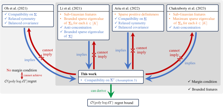
Figure 1: Illustration of relationships among distributional assumptions on context used in the sparse linear contextual bandit literature. The blue arrows represent implication relationships while the red arrows represent infeasible implication relationships. The conditions written in blue with the check bullet ✓ in the figure imply the compatibility on the optimal arm (Assumption 3), serving as sufficient conditions, while the conditions written in orange indicate additional assumptions necessary to achieve the existing methods’ regret guarantees, but not needed by our analysis. The case where all sub-optimal arms are fixed serves as a counter-example for the infeasible implication relationships. We provide the proofs of the implication relationship in Appendix B which may be of independent interest.

Discussion of assumptions.

Assumption 1 is a standard regularity assumption commonly used in the sparse linear bandit literature (Bastani and Bayati, 2020; Hao et al., 2020b; Ariu et al., 2022; Li et al., 2022; Chakraborty et al., 2023). It indicates that both the context features and the true parameter are bounded.

Assumption 2 restricts the probability of the expected reward of the optimal arm being near to the sub-optimal arms. To our best knowledge, the margin condition in the bandit setting was first introduced in Goldenshluger and Zeevi (2013) and is widely used in linear bandit literature (Wang et al., 2018; Bastani and Bayati, 2020; Papini et al., 2021; Li et al., 2021; Bastani et al., 2021; Ariu et al., 2022; Chakraborty et al., 2023). Unlike the minimum gap condition (Abbasi-Yadkori et al., 2011; Papini et al., 2021), which prohibits the instantaneous gap to be smaller than a fixed constant, the margin condition allows a probability of a small gap. The case where $\alpha=0$ imposes no additional constraints, while the case where $\alpha=\infty$ is equivalent to the minimum gap condition. The margin condition with general $\alpha$ smoothly bridges the cases with and without the minimum gap.

Assumption 3 is related to the compatibility condition used to guarantee the convergence property of sparse estimator in the high-dimensional statistic literature (Bühlmann and Van De Geer, 2011). Since the compatibility condition ensures that the Lasso estimator approaches its true value as the number of samples grows large, many pieces of high-dimensional bandit literature (Wang et al., 2018; Kim and Paik, 2019; Bastani and Bayati, 2020; Oh et al., 2021; Ariu et al., 2022) assume the condition. Kim and Paik (2019); Oh et al. (2021); Ariu et al. (2022) assume the compatibility condition on $\boldsymbol{\Sigma}:=\frac{1}{K}\mathbb{E}[\sum_{k}\mathbf{x}_{t,k}\mathbf{x}_{t,k}^{\top}]$. Li et al. (2021) assume the minimum sparse eigenvalue of the expected Gram matrix of the optimal arm when the instantaneous gap is greater than a constant $\Delta_{*}$, whose definition slightly differs from ours. Unlike previous works, we assume the compatibility condition only on the optimal arm without any constraints. Under this assumption, a theoretical guarantee about the convergence of the Lasso estimator can be derived only if the sufficient selections of the optimal arms is guaranteed, which necessitates more technical analysis. On the other hand, most of the previous work in sparse linear bandit that achieves poly-logarithmic regret under the margin condition implicitly assumes Assumption 3, indicating that our assumptions are strictly weaker than others. For instance, Oh et al. (2021); Ariu et al. (2022) assume relaxed symmetry and balanced covariance of the context feature, while other literature, such as Li et al. (2021); Chakraborty et al. (2023) assume an anti-concentration condition of the feature vectors. These conditions imply that estimation error reduces when data is obtained by a greedy policy, or in some case, any policy. Since choosing the optimal arm is also a greedy policy with respect to the true parameter, their assumptions imply ours, therefore our assumption is strictly weaker than the ones in the relevant literature with a single parameter setting. For detailed discussion about Assumption 3, refer to Appendix B.

3 Forced Sampling then Weighted Loss Lasso

3.1 Algorithm: FS-WLasso

Algorithm 1 FS-WLasso (Forced-Sampling then Weighted Loss Lasso)

1:Input: Number of exploration $M_{0}$, Weight $w$, Regularization parameters $\{\lambda_{t}\}_{t\geq 0}$

2:for $t=1,2,...,T$ do

3:     Observe $\{\mathbf{x}_{t,k}\}_{k=1}^{K}$

4:     if $t\leq M_{0}$ then $\triangleright$ Forced sampling stage

5:         Choose $a_{t}\sim\text{Unif}(\mathcal{A})$ and observe $r_{t,a_{t}}$

6:     else$\triangleright$ Greedy selection stage

7:         Compute $\hat{\boldsymbol{\beta}}_{t-1}$ as in (1)

8:         Select $a_{t}=\mathop{\mathrm{argmax}}_{k\in[K]}\mathbf{x}_{t,k}^{\top}\hat{\boldsymbol{\beta}}_{t-1}$ and observe $r_{t,a_{t}}$

9:     end if

10:end for

In this section, we present FS-WLasso (Forced Sampling then Weighted Loss Lasso) that adapts the forced-sampling technique (Goldenshluger and Zeevi, 2013; Bastani and Bayati, 2020). FS-WLasso consists of two stages: Forced sampling stage & Greedy selection stage. First, during the Forced sampling stage the agent chooses an arm uniformly at random for $M_{0}$ rounds. Then, for $t$ in the Greedy selection stage, the agent computes the Lasso estimator given by

$$\hat{\boldsymbol{\beta}}_{t-1}=\mathop{\mathrm{argmin}}_{\boldsymbol{\beta}}wL_{0}(\boldsymbol{\beta})+L_{t-1}(\boldsymbol{\beta})+\lambda_{t-1}\|\boldsymbol{\beta}\|_{1}\,,$$ (1)

where $L_{0}(\boldsymbol{\beta}):=\sum_{i=1}^{M_{0}}(\mathbf{x}_{i,a_{i}}^{\top}\boldsymbol{\beta}-r_{i,a_{i}})^{2}$ is the sum of squared errors over the samples acquired through random sampling, $L_{t-1}(\boldsymbol{\beta}):=\sum_{i=M_{0}+1}^{t-1}(\mathbf{x}_{i,a_{i}}^{\top}\boldsymbol{\beta}-r_{i,a_{i}})^{2}$ is the sum of squared errors over the samples observed in the Greedy selection stage, $w$ is the weight between the two loss functions, and $\lambda_{t-1}>0$ is the regularization parameter. The agent chooses the arm that maximizes the inner product of the feature vector and the Lasso estimator. FS-WLasso is summarized in Algorithm 1.

Remark 1.

Both FS-WLasso and ESTC (Hao et al., 2020b) have exploration stages, where the agent randomly selects arms for some initial rounds. However, the commit stages are very different. ESTC estimates the reward parameter only using the samples obtained during the exploration stage and does not update the parameters during the commit stage, whereas FS-WLasso continues to update the parameter using the samples obtained during the greedy selection stage. Therefore, our algorithm demonstrates superior statistical performance, achieving lower regret (and thus higher reward) by fully utilizing all accessible data.

Remark 2.

The minimization problem (1) takes the sum of squared errors, whereas the standard Lasso estimator takes the average. While $\lambda_{t}$ is typically chosen to be proportional to $\sqrt{1/t}$ in the existing literature (Bastani and Bayati, 2020; Oh et al., 2021; Ariu et al., 2022; Li et al., 2021), this slight difference leads to $\lambda_{t}$ being proportional to $\sqrt{t}$ in Theorems 1 and 2.

3.2 Regret Bound of FS-WLasso

Definition 1 (Compatibility constant ratio).

Let $\boldsymbol{\Sigma}:=\frac{1}{K}\mathbb{E}[\sum_{k\in[K]}\mathbf{x}_{t,k}\mathbf{x}_{t,k}^{\top}]$ be the expected Gram matrix of the averaged arm. We define the constant $\rho:=\phi_{*}^{2}/\phi^{2}(\boldsymbol{\Sigma},S_{0})$ as the ratio of the compatibility constant for $\boldsymbol{\Sigma}^{*}$ to compatibility constant for $\boldsymbol{\Sigma}$.

Remark 3.

By the definition of $\boldsymbol{\Sigma}$, it holds that $\boldsymbol{\Sigma}=\frac{1}{K}\mathbb{E}[\mathbf{x}_{t,a_{t}^{*}},\mathbf{x}_{t,a_{t}^{*}}^{\top}]+\frac{1}{K}\mathbb{E}[\sum_{k\neq a_{t}^{*}}\mathbf{x}_{t,k}\mathbf{x}_{t,k}^{\top}]\succeq\frac{1}{K}\mathbb{E}[\mathbf{x}_{t,a_{t}^{*}},\mathbf{x}_{t,a_{t}^{*}}^{\top}]$, which implies $\phi^{2}(\boldsymbol{\Sigma},S_{0})\geq\phi^{2}(\boldsymbol{\Sigma}^{*},S_{0})/K\geq\phi_{*}^{2}/K>0$. Hence, $\rho$ is well-defined with $0<\rho\leq K$.

Clearly, the compatibility conditions on the optimal arm implies the compatibility condition on the average arm. However, it is important to note that under the margin condition the entire stochastic context assumption (e.g., the compatibility condition along with additional diversity assumptions) in the previous literature imply the compatibility condition on the optimal arm, as clearly illustrated in Figure 1.

We present the regret upper bound of Algorithm 1. A formal version of the theorem and proof are deferred to Appendix C.2

Theorem 1 (Regret Bound of FS-WLasso).

Suppose Assumptions 1-3 hold. For $\delta\in(0,1]$, let $\tau$ be a constant that depends on $x_{\max},s_{0},\phi_{*},\sigma,\alpha,\Delta_{*},\log d,\log\delta$. If we set the input parameters of Algorithm 1 by

$$M_{0}=\bar{C}_{1}\max\big{\{}\rho^{2}x_{\max}^{4}s_{0}^{2}\phi_{*}^{-4}\log(d/\delta)\,,\rho^{2}\sigma^{2}x_{\max}^{4+\frac{4}{\alpha}}s_{0}^{2+\frac{2}{\alpha}}\Delta_{*}^{-2}\phi_{*}^{-4-\frac{4}{\alpha}}\left(\log\log\tau+\log(d/\delta)\right)\big{\}}\,,$$

$$\lambda_{t}=\bar{C}_{2}\sigma x_{\max}\bigg{(}\sqrt{(t-M_{0})\log\left(d(\log(t-M_{0}))^{2}/\delta\right)}+\sqrt{w^{2}M_{0}\log(d/\delta)}\bigg{)}\,,w=\sqrt{\tau/M_{0}}\,,$$

for some universal constants $\bar{C}_{1},\bar{C}_{2}>0$, then with probability at least $1-\delta$, Algorithm 1 achieves the following cumulative regret:

$$R(T)\leq 2x_{\max}bM_{0}+I_{\tau}+I_{T}\,,$$

where $I_{\tau}=\mathcal{O}\left(\sigma^{2}\Delta_{*}^{-1}\left(x_{\max}^{2}s_{0}/\phi_{*}^{2}\right)^{1+\frac{1}{\alpha}}\log(d/\delta)\right)$ and

$$I_{T}=\begin{cases}\mathcal{O}\left(\frac{\left(\sigma x_{\max}^{2}s_{0}/\phi_{*}^{2}\right)^{1+\alpha}}{\Delta_{*}^{\alpha}(1-\alpha)}T^{\frac{1-\alpha}{2}}\left(\log d+\log\frac{\log T}{\delta}\right)^{\frac{1+\alpha}{2}}\right)&\text{ for }\alpha\in\left(0,1\right)\,,\\ \mathcal{O}\left(\frac{\left(\sigma x_{\max}^{2}s_{0}/\phi_{*}^{2}\right)^{2}}{\Delta_{*}}\log{T}\left(\log d+\log\frac{\log T}{\delta}\right)\right)&\text{ for }\alpha=1\,,\\ \mathcal{O}\left(\frac{\alpha}{(\alpha-1)^{2}}\cdot\frac{\sigma^{2}\left(x_{\max}^{2}s_{0}/\phi_{*}^{2}\right)^{1+\frac{1}{\alpha}}}{\Delta_{*}}\left(\log d+\log\frac{1}{\delta}\right)\right)&\text{ for }1<\alpha\leq\infty\,.\end{cases}$$

Discussion of Theorem 1.

In terms of key problem instances ($s_{0},d$, and $T$), Theorem 1 establishes the regret bounds that scale poly-logarithmically on $d$ and $T$, specifically, $\mathcal{O}(s_{0}^{\alpha+1}T^{\frac{1-\alpha}{2}}(\log d+\log\log T)^{\frac{\alpha+1}{2}})$ for $\alpha\in(0,1)$, $\mathcal{O}(s_{0}^{2}\log T(\log d+\log\log T))$ for $\alpha=1$, and $\mathcal{O}(s_{0}^{2+\frac{2}{\alpha}}\log d)$ for $\alpha>1$.  Li et al. (2021) constructs a regret lower bound of $\mathcal{O}(T^{\frac{1-\alpha}{2}}\left(\log d\right)^{\frac{\alpha+1}{2}}+\log T)$ when $\alpha\in[0,1]$, which our algorithm achieves up to a $\log T$ factor. The expected regret for Algorithm 1 also can be obtained by taking $\delta=1/T$. For the $T$-agnostic setting, we derive FS-Lasso, which uses forced samples adaptively, and establish the same regret bound as in Theorem 1 (Appendix D).

Existing Lasso bandit literature that achieves $\mathcal{O}(\text{poly}\log dT)$ regret under the single parameter setting necessitates stronger assumptions on the context distribution (e.g., relaxed symmetry & balanced covariance or anti-concentration), which are non-verifiable in practical scenarios. In addition, when context distributions do not satisfy the strong assumptions employed in the previous literature, the existing algorithms can critically undermine regret performance, with no recourse for adjustment nor guarantees provided. That is, there is nothing one can do when such strong context assumptions are not satisfied in the existing literature. However, we show that the compatibility condition only on the optimal arm is sufficient to achieve poly-logarithmic regret under the margin condition, and demonstrate that our assumption is strictly weaker than those used in other Lasso bandit literature under the single parameter setting.

Our result also improves the known regret bound for low-dimensional setting, where $s_{0}$ may be replaced with $d$. In this case, Assumption 3 becomes equivalent to the HLS condition (Hao et al., 2020a; Papini et al., 2021). Under the HLS condition and the minimum gap condition, Papini et al. (2021) show that LinUCB achieves a constant regret bound independent of $T$ with high probability. However, when the margin condition (Assumption 2) is assumed, their result guarantees $O(\log T)$ regret bound only when $\alpha>2$. Our algorithm achieves a constant regret bound with high probability when $\alpha>1$, expanding the range of $\alpha$ that the constant regret is attainable.

Remark 4.

In practice, $M_{0}$ in Algorithm 1 is a tunable hyper-parameter. Similar hyper-parameters exist in many of the previous Lasso-based bandit algorithms (Bastani and Bayati, 2020; Hao et al., 2020b; Li et al., 2021; Oh et al., 2021; Ariu et al., 2022; Chakraborty et al., 2023). Although $M_{0}$ theoretically depends on $s_{0}$, $\rho$ and sub-Gaussian parameter $\sigma$ in Theorem 1, we however do not need to specify each of those problem parameters separately in practice. Rather, $M_{0}$ is tuned as a whole. Theorem 2 suggests that small $M_{0}$ may suffices by presenting a setting where $M_{0}=0$ is valid. Furthermore, we observe that that our algorithm is not sensitive to the choice of $M_{0}$ in numerical experiments. Refer to Appendix G for more details.

In most sparse linear bandit algorithm regret analyses under the single parameter setting (Kim and Paik, 2019; Li et al., 2021; Oh et al., 2021; Ariu et al., 2022; Chakraborty et al., 2023), the maximum regret is incurred during the burn-in phase, where the compatibility condition of the empirical Gram matrix is not guaranteed. The compatibility condition after the burn-in phase is ensured by additional diversity assumptions on context features (e.g., anti-concentration (Li et al., 2021; Chakraborty et al., 2023), relaxed symmetry & balanced covariance (Oh et al., 2021; Ariu et al., 2022)), rather than explicit exploration of the algorithms. Therefore, the Lasso estimator calculation (Oh et al., 2021; Ariu et al., 2022) or explicit exploration (UCB in Li et al. (2021) or TS in Chakraborty et al. (2023)) during their burn-in phases does not contribute to the regret bound.
On the other hand, our forced sampling stage does not compute parameters but acquires diverse samples without requiring diversity assumptions on context features beyond the compatibility condition on the optimal arm, making it more efficient during the burn-in phases. If additional diversity assumptions (Li et al., 2021; Oh et al., 2021; Ariu et al., 2022; Chakraborty et al., 2023) are also applied to our algorithm, we show that $\mathcal{O}(\text{poly}\log T)$ regret is achieved without the forced sampling stage in Algorithm 1.

Theorem 2.

Suppose that Assumptions 1-3 hold, and further assume either the anti-concentration (Assumption 4) or relaxed symmetry & balanced covariance (Assumption 6-8) assumptions. Let $\phi_{\text{G}}$ be an appropriate constant that is determined by the employed assumptions, and $\tau$ be a constant that depends on $\sigma$, $x_{\max}$, $s_{0}$, $\Delta_{*}$, $\phi_{*}$, $\phi_{\text{G}}$, $\alpha$, $\log d$, and $\log\delta$. If we set the input parameters of Algorithm 1 by $M_{0}=0$, i.e. no forced-sampling stage, and $\lambda_{t}=\bar{C}_{2}\sigma x_{\max}\sqrt{t\log\left(d(\log t)^{2}/\delta\right)}$, where $\bar{C}_{2}$ is the same universal constant as in Theorem 1, then with probability at least $1-\delta$, Algorithm 1 achieves the following cumulative regret with probability at least $1-\delta$:

$$R(T)\leq\begin{cases}I_{b}+I_{2}(T)&T\leq\tau\\ I_{b}+I_{2}(\tau)+I_{T}&T>\tau\,,\end{cases}$$

where $I_{T}$ takes the same value as in Theorem 1, and

$$I_{b}=\mathcal{O}\left(x_{\max}^{5}bs_{0}^{2}\phi^{-4}_{\text{G}}\left(\log(x_{\max}s_{0}\phi^{-1}_{\text{G}})+\log d-\log\delta\right)\right)\,,$$

$$I_{2}(T)=\begin{cases}\mathcal{O}\left(\frac{\left(\sigma x_{\max}^{2}s_{0}/\phi_{\text{G}}^{2}\right)^{1+\alpha}}{\Delta_{*}^{\alpha}(1-\alpha)}T^{\frac{1-\alpha}{2}}\left(\log d+\log\frac{\log T}{\delta}\right)^{\frac{1+\alpha}{2}}\right)&\text{ for }\alpha\in\left[0,1\right)\,,\\ \mathcal{O}\left(\frac{\left(\sigma x_{\max}^{2}s_{0}/\phi_{\text{G}}^{2}\right)^{2}}{\Delta_{*}}\log{T}\left(\log d+\log\frac{\log T}{\delta}\right)\right)&\text{ for }\alpha=1\,,\\ \mathcal{O}\left(\frac{\alpha^{2}}{(\alpha-1)^{2}}\cdot\frac{\left(\sigma x_{\max}^{2}s_{0}/\phi_{\text{G}}^{2}\right)^{2}}{\Delta_{*}}\left(\log d+\log\frac{1}{\delta}\right)\right)&\text{ for }1<\alpha\leq\infty\,.\end{cases}$$

Discussion of Theorem 2.

Theorem 2 offers that random exploration of Algorithm 1 may not be required if the additional diversity assumptions on context features are given. This result indicates that the number of exploration may be tuned according to the specific problem instance. The assumptions of the Theorem 2 are still weaker than, or equally strong as Oh et al. (2021); Li et al. (2021); Chakraborty et al. (2023), while the regret bounds are not greater than theirs. We slightly improve the regret bound of Li et al. (2021) when $1<\alpha\leq\infty$. Specifically, a term proportional to $s_{0}^{2}/(\Delta_{*}\phi_{*}^{4})$ in Li et al. (2021) is sharpened to $s_{0}^{1+\frac{1}{\alpha}}/(\Delta_{*}\phi_{*}^{2+\frac{2}{\alpha}})$ in our result. We also achieve a tighter regret bound than Chakraborty et al. (2023), which is proportional to $K^{4}$. Our result is proportional to at most $K^{2}$ since $\phi_{*}^{2}\geq\Omega(\frac{1}{K})$ holds under their assumptions, which is shown in Lemma 1.

3.3 Sketch of Proofs

To establish the regret bounds stated in Theorems 1 and 2, we design a novel high-probability analysis that utilizes mathematical induction. Under our assumptions, a small estimation error of $\hat{\boldsymbol{\beta}}_{t}$ is ensured when the optimal arms have been chosen a sufficient number of times. On the other hand, the small estimation error results in a higher probability of choosing the optimal arm at the next round. This observation reveals the cyclic structure regarding the selection of the optimal arms. We observe that it is not a circular reasoning, but is a domino-like phenomenon that propagates forward in time. Existing methods of analyzing the sparse linear bandits (Bastani and Bayati, 2020; Oh et al., 2021; Li et al., 2021; Ariu et al., 2022; Chakraborty et al., 2023) fail to capture this phenomenon. Those methods have difficulties handling the strong dependencies across the selected arms, since they rely on automatic exploration facilitated by the diversity conditions, regardless of the previously selected arms. We meticulously analyze the cyclic structure of the good events and derive a novel mathematical induction argument that guarantees that the good events hold true indefinitely with a small probability of failure, where the good events are described by small estimation errors and small numbers of sub-optimal arms selections.

There are three main difficulties that lie in the way of constructing the induction argument. First, the initial condition of the induction must be satisfied, in other words, the cycle must begin. We guarantee the initial condition through random exploration (Theorem 1) or additional diversity assumptions (Theorem 2). We show that after the initial stages, the algorithm attains a sufficiently accurate estimator, which starts the cycle. Second, the algorithm must be able to propagate the good event to the next round. A small estimation error does not always guarantee the choice of the optimal arm. Instead, we show that it induces a bounded ratio of sub-optimal selections through time. The compatibility condition on the optimal arms implies that if the optimal arms constitute a large portion of observed data, the algorithm attains a small estimation error. We build an induction argument upon these relationships. Lastly, due to the stochastic nature of the problem, the algorithm suffers a small probability of failing to propagate the good event at every round. Without careful analysis, the sum of such probabilities easily exceeds 1, invalidating the whole proof. We bound the sum to be small by carefully constructing high-probability events that occur independently of the induction argument, then prove that the induction argument always holds under the events. The complete proof is illustrated in Appendix C.

4 Numerical Experiments

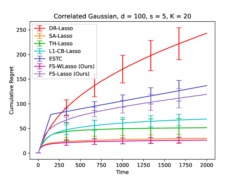
(a) Experiment 1

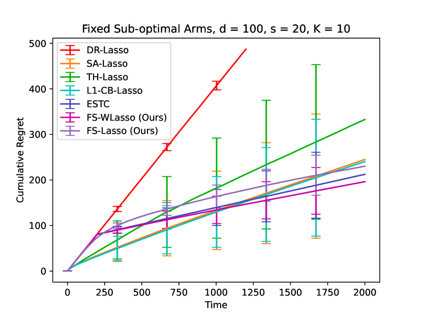
(b) Experiment 2

Figure 2: The evaluations of Lasso bandit algorithms under a single parameter setting are presented. Figure 2(a) shows results where all context feature vectors are sampled from a correlated Gaussian distribution. Figure 2(b) shows results where the context feature vectors of sub-optimal arms are fixed throughout time, and only the feature vector of the optimal arm has randomness.

We perform numerical evaluations on synthetic datasets. We compare our algorithms, FS-WLasso and FS-Lasso, with sparse linear bandit algorithms including DR Lasso Bandit (Kim and Paik, 2019), SA Lasso BANDIT (Oh et al., 2021), TH Lasso Bandit (Ariu et al., 2022), $\ell_{1}$-Confidence Ball Based Algorithm (L1-CB-Lasso) (Li et al., 2021), and ESTC (Hao et al., 2020b). We plot the mean and standard deviation of cumulative regret across 100 runs for each algorithm.

The results clearly demonstrate that our proposed algorithms outperform the existing sparse linear bandit methods we evaluated. In particular, even in cases where the context features of all arms, except for the optimal arm, are fixed (rendering assumptions such as anti-concentration invalid), our proposed algorithms surpass the performance of existing ones. More details are presented in Appendix F.

5 Conclusion

In this work, we study the stochastic context conditions under which the Lasso bandit algorithm can achieve a poly-logarithmic regret. We present rigorous comparisons on the relative strengths of the conditions utilized in the sparse linear bandit literature, which provide insights that can be of independent interest. Our regret analysis shows that the proposed algorithms establish a poly-logarithmic dependency on the feature dimension and time horizon.

Appendix A Notations & Definitions

We introduce some additional notations that are necessary for the analysis. Denote $\text{reg}_{t}=\mathbf{x}_{t,a_{t}^{*}}^{\top}\boldsymbol{\beta}^{*}-\mathbf{x}_{t,a_{t}}^{\top}\boldsymbol{\beta}^{*}$ as the instantaneous regret at time $t$. For $I\subset[d]$, define $\mathbb{C}(I)$ to be the set $\left\{\mathbf{v}\in\mathbb{R}^{d}:\|\mathbf{v}_{I^{\mathsf{c}}}|_{1}\leq 3\|\mathbf{v}_{I}\|_{1}\right\}$. Then, the definition of compatibility constant in Assumption 3 can be rewritten as $\phi^{2}(\mathbf{M},I)=\inf_{\mathbf{v}\in\mathbb{C}(I)\setminus\{\mathbf{0}_{d}\}}\frac{s_{0}\mathbf{v}^{\top}\mathbf{M}\mathbf{v}}{\|\mathbf{v}_{I}\|_{1}^{2}}$. We define the probability space $(\Omega,\mathcal{F},\mathbb{P})$, where $\Omega$ is the sample space, $\mathcal{F}$ is the event set, and $\mathbb{P}$ is the probability measure.

We provide tables of notations used in this paper. Table 2 organizes the notations related to the problem of this paper with proper sub-categories. We present the notations generally used beyond the field of this paper in Table 3.

Table 2: Table of notions specific to this paper

Linear Bandit
$\boldsymbol{\beta}^{*}$	True parameter vector
$\mathbf{x}_{t,k}$	Context feature vector at time $t$, arm $k$
$\mathcal{X}$	Set of all possible context feature vectors
$\mathcal{D}_{\mathcal{X}}$	Distribution of context vectors tuple $\{\mathbf{x}_{t,k}\}_{k=1}^{K}$
$a_{t}$	Chosen arm at time $t$
$a_{t}^{*}$	Optimal arm at time $t$
$\eta_{t}$	Zero-mean sub-Gaussian noise at time $t$
$\sigma$	Variance proxy of $\eta_{t}$
$r_{t,a_{t}}$	Observed reward at time $t$
$\text{reg}_{t}$	Instantaneous regret at time $t$
$d$	Dimension of feature and true parameter vectors
$K$	Number of arms
$T$	Time horizon
High-Dimensional Statistics
$S_{0}$	Active set, i.e. $\left\{j\in[d]:\left(\boldsymbol{\beta}^{*}\right)_{j}\neq 0\right\}$
$s_{0}$	Sparsity index, $\left|S_{0}\right\|$
$v_{j,S_{0}}$	$v_{j}\mathds{1}\left\{j\in S_{0}\right\}$
$\mathbf{v}_{S_{0}}$	$[v_{1,S_{0}},\ldots,v_{d,S_{0}}]^{\top}$
$\mathbf{v}_{S_{0}^{\mathsf{c}}}$	$\mathbf{v}_{[d]\setminus S_{0}}$
$\mathbb{C}(S_{0})$	$\left\{\mathbf{v}\in\mathbb{R}^{d}:\|\mathbf{v}_{S_{0}^{\mathsf{c}}}\|_{1}\leq 3\|\mathbf{v}_{S_{0}}\|_{1}\right\}$
$\phi^{2}\left(\mathbf{M},S_{0}\right)$	Compatibility constant of matrix $\mathbf{M}$ over set $S_{0}$
Assumptions
$x_{\max}$	$\ell_{\infty}$ norm upper bound of $\mathbf{x}\in\mathcal{X}$
$b$	$\ell_{1}$ norm upper bound of $\boldsymbol{\beta}^{*}$
$\Delta_{t}$	Instantaneous gap, i.e. $\max_{a\neq a_{t}^{*}}\mathbf{x}_{t,a_{t}^{*}}^{\top}\boldsymbol{\beta}^{*}-\mathbf{x}_{t,a}^{\top}\boldsymbol{\beta}^{*}$
$\Delta_{*}$	Margin constant, or relaxed minimum gap
$\alpha$	Margin condition parameter
$\mathbf{x}_{*}$	Optimal arm feature as random vector
$\boldsymbol{\Sigma}^{*}$	Expected Gram matrix of optimal arm, i.e. $\mathbb{E}\left[\mathbf{x}_{*}\mathbf{x}_{*}^{\top}\right]$
$\phi_{*}$	Lower bound of $\phi^{2}\left(\boldsymbol{\Sigma}^{*},S_{0}\right)$
Algorithm
$M_{0}$	Number of random exploration rounds
$w$	Weight between square errors of random samples and greedy samples
$\lambda_{t}$	Lasso regularization parameter
$\hat{\boldsymbol{\beta}}_{t}$	Lasso estimate of $\boldsymbol{\beta}^{*}$
Analysis
$\delta$	Probability of failure
$\boldsymbol{\Sigma}$	Theoretical Gram matrix of all arms, i.e. $\frac{1}{K}\mathbb{E}\left[\sum_{k=1}^{K}\mathbf{x}_{t,k}\mathbf{x}_{t,k}^{\top}\right]$
$\boldsymbol{\Sigma}_{\Gamma}^{*}$	Theoretical Gram matrix of optimal arm with large gap, $\mathbb{E}\left[\mathbf{x}_{*}\mathbf{x}_{*}\mid\Delta_{t}>\Delta_{*}\right]$
$\boldsymbol{\Sigma}_{k}$	Theoretical Gram matrix of arm $k$, i.e. $\mathbb{E}\left[\mathbf{x}_{t,k}\mathbf{x}_{t,k}^{\top}\right]$
$\rho$	Compatibility constant ratio
$\hat{\mathbf{V}}_{M_{0}+\tau}$	(Weighted) Empirical Gram matrix, $\sum_{t=1}^{M_{0}}w\mathbf{x}_{t,a_{t}}\mathbf{x}_{t,a_{t}}^{\top}+\sum_{t=M_{0}+1}^{M_{0}+\tau}\mathbf{x}_{t,a_{t}}\mathbf{x}_{t,a_{t}}^{\top}$
$N_{\tau_{1}}(t^{\prime})$	Number of sub-optimal selections during $t=M_{0}+\tau_{1}+1$ to $M_{0}+\tau_{1}+t^{\prime}$
$\overline{\Delta}_{t}$	Upper bound of $2x_{\max}\|\boldsymbol{\beta}^{*}-\hat{\boldsymbol{\beta}}_{t}\|_{1}$
$\mathcal{F}_{t}$	$\sigma$-algebra generated by $\{\mathbf{x}_{\tau,i}\}_{\tau\in[t],i\in[K]},\{a_{\tau}\}_{\tau\in[t]},\{r_{\tau,a_{\tau}}\}_{\tau\in[t-1]}$
$\mathcal{F}_{t}^{+}$	$\sigma$-algebra generated by $\{\mathbf{x}_{\tau,i}\}_{\tau\in[t],i\in[K]},\{a_{\tau}\}_{\tau\in[t]},\{r_{\tau,a_{\tau}}\}_{\tau\in[t]}$

Table 3: Table of generic notations

Sets and functions
$\mathbb{N}$	Set of natural numbers, starting with $1$
$\mathbb{N}_{0}$	Set of natural numbers, together with $0$
$[N]$	Set of natural numbers up to $N$, i.e. $\left\{1,2,\ldots,N\right\}$
$\mathbb{R}$	Set of real numbers
$\mathbb{R}_{\geq 0}$	Set of non-negative real numbers
$\mathds{1}$	Indicator function
Vector and matrices
$\|\cdot\|_{0}$	$\ell_{0}$ norm of a vector, i.e. number of non-zero elements
$\|\cdot\|_{2}$	$\ell_{2}$ norm of a vector
$\|\cdot\|_{\infty}$	$\ell_{\infty}$ norm of a vector or a matrix, i.e. maximum absolute value of elements
$(\cdot)_{j}$	$j$-th element of a vector
$(\cdot)_{ij}$	$ij$-th element of a matrix
$\mathbf{0}_{d}$	Zero vector in $\mathbb{R}^{d}$
$\mathbf{I}_{d}$	Identity matrix in $\mathbb{R}^{d\times d}$
Probability
$\left(\Omega,\mathcal{F},\mathbb{P}\right)$	Probability space
$\mathbb{E}$	Expectation

Appendix B Discussion for the Compatibility Condition on the Optimal Arm (Assumption 3)

We introduce some of the assumptions made in related works about sparse linear bandit. We show that these assumptions imply Assumption 3, proving that our assumptions are strictly weaker than others.

Assumption 4 (Anti-concentration (Li et al., 2021; Chakraborty et al., 2023)).

There exists a positive constant $\xi$ such that for each $k\in[K]$, $t\in[T]$, $\mathbf{v}\in\left\{\mathbf{u}\in\mathbb{R}^{d}\mid\left\|\mathbf{u}\right\|_{0}\leq C_{d}\right\}$, and $h>0$, $\mathbb{P}((\mathbf{x}_{t,k}^{\top}\mathbf{v})^{2}\leq h\|\mathbf{v}\|_{2}^{2})\leq\xi h$. $C_{d}$ equals $d$ in Li et al. (2021) and is a big enough constant that depends on $\xi$, $K$, $s_{0}$ and more in Chakraborty et al. (2023).

Assumption 5 (Sparse eigenvalue of the optimal arm (Li et al., 2021)).

Let $\Gamma=\left\{\omega\in\Omega:\Delta_{t}\geq 2^{-\frac{1}{\alpha}}\Delta_{*}\right\}$ be the event that the instantaneous gap is large enough, and $\boldsymbol{\Sigma}_{\Gamma}^{*}=\mathbb{E}\left[\mathbf{x}_{t}^{*}{\mathbf{x}_{t}^{*}}^{\top}\mid\Gamma\right]$ be the expected Gram matrix of the optimal arm conditioned on the event $\Gamma$. Then, there exists a constant $\phi_{1}>0$ such that

$$\inf_{\begin{subarray}{c}\mathbf{v}\in\mathbb{R}^{d}\setminus\left\{\mathbf{0}_{d}\right\}\\ \left\|\mathbf{v}\right\|_{0}\leq C^{*}s_{0}+1\end{subarray}}\frac{\mathbf{v}^{\top}\boldsymbol{\Sigma}_{\Gamma}^{*}\mathbf{v}}{\left\|\mathbf{v}\right\|_{2}^{2}}\geq\phi_{1}^{2}\,,$$ (2)

where $C^{*}$ is a big enough constant that depends on $\xi$ (in Assumption 4), $K$, and more.

Assumption 6 (Compatibility condition on the averaged arm (Oh et al., 2021; Ariu et al., 2022)).

Let $\boldsymbol{\Sigma}=\mathbb{E}_{\left\{\mathbf{x}_{t,k}\right\}_{k=1}^{K}\sim\mathcal{D}_{\mathcal{X}}}\left[\frac{1}{K}\sum_{k=1}^{K}\mathbf{x}_{t,k}\mathbf{x}_{t,k}^{\top}\right]$ be the expected Gram matrix of the averaged arm. Then there exists a constant $\phi_{2}>0$ such that $\phi^{2}\left(\boldsymbol{\Sigma},S_{0}\right)\geq\phi_{2}$.

Assumption 7 (Relaxed symmetry (Oh et al., 2021; Ariu et al., 2022)).

For the context distribution $\mathcal{P}_{\mathcal{X}}$, there exists a constant $1\leq\nu<\infty$ such that $0<\frac{\mathcal{P}_{\mathcal{X}}(-\mathbf{x})}{\mathcal{P}_{\mathcal{X}}(\mathbf{x})}\leq\nu$ for any $\mathbf{x}\in\mathcal{X}$ with $\mathcal{P}_{\mathcal{X}}(\mathbf{x})\neq 0$.

Assumption 8 (Balanced covariance (Oh et al., 2021; Ariu et al., 2022)).

There exists $0<C_{\mathcal{X}}<\infty$ such that for any permutation $(i_{1},\ldots,i_{K})$ of $(1,\ldots,K)$, any $k\in\{2,\ldots,K-1\}$, and any fixed $\boldsymbol{\beta}\in\mathbb{R}^{d}$, it holds that

$$\mathbb{E}\left[\mathbf{x}_{i_{k}}\mathbf{x}_{i_{k}}^{\top}\mathds{1}\{\mathbf{x}_{i_{1}}^{\top}\boldsymbol{\beta}<\ldots<\mathbf{x}_{i_{K}}^{\top}\boldsymbol{\beta}\}\right]\preceq C_{\mathcal{X}}\mathbb{E}\left[(\mathbf{x}_{i_{1}}\mathbf{x}_{i_{1}}^{\top}+\mathbf{x}_{i_{K}}\mathbf{x}_{i_{K}}^{\top})\mathds{1}\{\mathbf{x}_{i_{1}}^{\top}\boldsymbol{\beta}<\ldots<\mathbf{x}_{i_{K}}^{\top}\boldsymbol{\beta}\}\right]\,.$$

We show that some of the assumptions imply the following property, which we name the greedy diversity.

Definition 2 (Greedy diversity).

For any fixed $\boldsymbol{\beta}\in\mathbb{R}^{d}$, define the greedy policy with respect to an estimator $\boldsymbol{\beta}$ as $\pi_{\boldsymbol{\beta}}\left(\left\{\mathbf{x}_{k}\right\}_{k=1}^{K}\right)=\mathop{\mathrm{argmax}}_{k\in[K]}\mathbf{x}_{k}^{\top}\boldsymbol{\beta}$. Denote the chosen feature vector with respect to the greedy policy as $\mathbf{x}_{\boldsymbol{\beta}}=\mathbf{x}_{\pi_{\boldsymbol{\beta}}\left(\left\{\mathbf{x}_{k}\right\}_{k=1}^{K}\right)}$. The context distribution $\mathcal{D}_{\mathcal{X}}$ satisfies the greedy diversity if there exists a constant $\phi_{\text{G}}>0$ such that for any $\boldsymbol{\beta}\in\mathbb{R}^{d}$,

$$\phi^{2}\left(\mathbb{E}_{\left\{\mathbf{x}_{k}\right\}_{k=1}^{K}\sim\mathcal{D}_{\mathcal{X}}}\left[\mathbf{x}_{\boldsymbol{\beta}}{\mathbf{x}_{\boldsymbol{\beta}}}^{\top}\right],S_{0}\right)\geq\phi_{\text{G}}^{2}\,.$$ (3)

Remark 5.

Note that $\mathbf{x}_{\boldsymbol{\beta}^{*}}=\mathbf{x}_{*}$. Under the greedy diversity, Assumption 3 holds with $\phi_{*}=\phi_{\text{G}}$ by plugging in $\boldsymbol{\beta}=\boldsymbol{\beta}^{*}$. Therefore, the greedy diversity implies the compatibility condition on the optimal arm.

Anti-concentration to ours:

The following lemma shows that anti-concentration implies the greedy diversity, hence it implies Assumption 3. While Li et al. (2021) and Chakraborty et al. (2023) use $\epsilon$-net argument to ensure the compatibility condition of the empirical Gram matrix, we follow a slightly different approach to ensure the compatibility condition of the expected Gram matrix. Another point to note is that Li et al. (2021); Chakraborty et al. (2023) employ additional assumptions, such as sub-Gaussianity of feature vectors and maximum sparse eigenvalue condition, to upper bound the diagonal elements of the empirical Gram matrix. To make the analysis simpler, we replace the upper bound by $x_{\max}^{2}$.

Lemma 1.

If Assumption 4 holds with $C_{d}\geq 64x_{\max}^{2}\xi Ks_{0}+1$, then the greedy diversity is satisfied with $\phi_{\text{G}}^{2}\geq\frac{1}{4\xi K}$.

Proof of Lemma 1.

We first show that $\mathbb{E}\left[\mathbf{x}_{\beta}\mathbf{x}_{\beta}^{\top}\right]$ has positive minimum sparse eigenvalue, then use the Transfer principle (Lemma 29) adopted in Li et al. (2021) and Chakraborty et al. (2023). Let $\mathbf{v}\in\mathbb{R}^{d}$ be a vector with $\left\|\mathbf{v}\right\|_{2}=1$ and $\left\|\mathbf{v}\right\|_{0}\leq C_{d}$. For a fixed value of $h\geq 0$, $\left({\mathbf{x}_{\beta}}^{\top}\mathbf{v}\right)^{2}\leq h$ implies that there exists at least one $k\in[K]$ such that $(\mathbf{x}_{k}^{\top}\mathbf{v})^{2}\leq h$ holds. Then, we infer that

$$\mathbb{P}\left(\left({\mathbf{x}_{\beta}}^{\top}\mathbf{v}\right)^{2}\leq h\right) \leq\mathbb{P}\left(\exists k\in[K]:(\mathbf{x}_{k}^{\top}\mathbf{v})^{2}\leq h\right)$$

$$\leq\sum_{k=1}^{K}\mathbb{P}\left((\mathbf{x}_{k}^{\top}\mathbf{v})^{2}\leq h\right)$$

$$\leq\xi Kh\,,$$

where the second inequality is the union bound, and the last inequality is from Assumption 4. Then, using that $\left({\mathbf{x}_{\beta}}^{\top}\mathbf{v}\right)^{2}=\mathbf{v}^{\top}\left({\mathbf{x}_{\beta}}{\mathbf{x}_{\beta}}^{\top}\right)\mathbf{v}$, we bound the minimum sparse eigenvalue of the expected Gram matrix.

$$\mathbb{E}\left[\mathbf{v}^{\top}\left({\mathbf{x}_{\beta}}{\mathbf{x}_{\beta}}^{\top}\right)\mathbf{v}\right] =\int_{0}^{\infty}\mathbb{P}\left(\mathbf{v}^{\top}\left({\mathbf{x}_{\beta}}{\mathbf{x}_{\beta}}^{\top}\right)\mathbf{v}\geq x\right)\,dx$$

$$\geq\int_{0}^{\frac{1}{\xi K}}\mathbb{P}\left(\mathbf{v}^{\top}\left({\mathbf{x}_{\beta}}{\mathbf{x}_{\beta}}^{\top}\right)\mathbf{v}\geq x\right)\,dx$$

$$\geq\int_{0}^{\frac{1}{\xi K}}(1-\xi Kx)\,dx$$

$$=\frac{1}{2\xi K}\,.$$ (4)

Now, we use the Transfer principle. Let $\hat{\boldsymbol{\Sigma}}=\mathbb{E}\left[\mathbf{x}_{\beta}\mathbf{x}_{\beta}^{\top}\right]$ and $\bar{\boldsymbol{\Sigma}}=\frac{1}{\xi K}\mathbf{I}_{d}$. Inequality (4) shows that for $\left\|\mathbf{v}\right\|_{0}\leq C_{d}$, it holds that

$$\mathbf{v}^{\top}\hat{\boldsymbol{\Sigma}}\mathbf{v}\geq\frac{1}{2}\mathbf{v}^{\top}\bar{\boldsymbol{\Sigma}}\mathbf{v}\,.$$

For any $j\in[d]$, we have $\hat{\boldsymbol{\Sigma}}_{jj}=\mathbb{E}\left[\left(\mathbf{x}_{\boldsymbol{\beta}}\right)_{j}^{2}\right]\leq x_{\max}^{2}$. Then the conditions of Lemma 29 hold with $\eta=\frac{1}{2}$, $\mathbf{D}=x_{\max}^{2}\mathbf{I}_{d}$, and $m=C_{d}$. Suppose $\mathbf{u}\in\mathbb{C}(S_{0})$. By Lemma 29, we have

$$\mathbf{u}^{\top}\mathbb{E}\left[\mathbf{x}_{\boldsymbol{\beta}}\mathbf{x}_{\boldsymbol{\beta}}^{\top}\right]\mathbf{u}\geq\frac{1}{2\xi K}\left\|\mathbf{u}\right\|_{2}^{2}-\frac{\left\|\mathbf{D}^{\frac{1}{2}}\mathbf{u}\right\|_{1}^{2}}{C_{d}-1}\,.$$ (5)

The first term is lower bounded as the following:

$$\frac{1}{2\xi K}\left\|\mathbf{u}\right\|_{2}^{2} \geq\frac{1}{2\xi K}\left\|\mathbf{u}_{S_{0}}\right\|_{2}^{2}$$

$$\geq\frac{1}{2\xi Ks_{0}}\left\|\mathbf{u}_{S_{0}}\right\|_{1}^{2}\,,$$ (6)

where the second inequality is the Cauchy-Schwarz inequality. The second term is upper bounded as the following:

$$\frac{\left\|\mathbf{D}^{\frac{1}{2}}\mathbf{u}\right\|_{1}^{2}}{C_{d}-1} =\frac{\left\|x_{\max}\mathbf{u}\right\|_{1}^{2}}{64x_{\max}^{2}\xi Ks_{0}}$$

$$=\frac{\left\|\mathbf{u}\right\|_{1}^{2}}{64\xi Ks_{0}}$$

$$\leq\frac{16\left\|\mathbf{u}_{S_{0}}\right\|_{1}^{2}}{64\xi Ks_{0}}$$

$$=\frac{\left\|\mathbf{u}_{S_{0}}\right\|_{1}^{2}}{4\xi Ks_{0}}\,,$$ (7)

where the inequality holds by $\left\|\mathbf{u}\right\|_{1}=\left\|\mathbf{u}_{S_{0}}\right\|_{1}+\|\mathbf{u}_{S_{0}^{\mathsf{c}}}\|_{1}\leq 4\left\|\mathbf{u}_{S_{0}}\right\|_{1}$ when $\mathbf{u}\in\mathbb{C}(S_{0})$. Putting inequalities (5), (6), and (7) together, we obtain

$$\mathbf{u}^{\top}\mathbb{E}\left[\mathbf{x}_{\boldsymbol{\beta}}\mathbf{x}_{\boldsymbol{\beta}}^{\top}\right]\mathbf{u}\geq\frac{\left\|\mathbf{u}_{S_{0}}\right\|_{1}^{2}}{4\xi Ks_{0}}\,,$$ (8)

which implies $\phi^{2}(\mathbb{E}\left[\mathbf{x}_{\beta}\mathbf{x}_{\beta}^{\top}\right],S_{0})\geq\frac{1}{4\xi K}$. ∎

Sparse eigenvalue to ours:

Assumption 5 does not imply the greedy diversity, but still implies compatibility condition on the optimal arm. As in the previous subsection, we replace the upper bound of the diagonal entries of the Gram matrix obtained in Li et al. (2021) with $x_{\max}^{2}$ for simpler analysis.

Lemma 2.

Suppose Assumptions 2, 4, and 5 hold with $C^{*}=64x_{\max}^{2}\xi K$. Then Assumption 3 holds with $\phi_{*}^{2}\geq\frac{\phi_{1}^{2}}{3}$.

Proof of Lemma 2.

Lemma 1 shows that Assumption 4 implies compatibility condition on the optimal arm with $\phi_{*}^{2}\geq\frac{1}{4\xi K}$. If $\frac{\phi_{1}^{2}}{3}\leq\frac{1}{4\xi K}$, then the proof is complete. Suppose $\frac{\phi_{1}^{2}}{3}\geq\frac{1}{4\xi K}$.
By the margin condition, the probability of the event $\Gamma$ is at least $\mathbb{P}\left(\Gamma\right)=1-\mathbb{P}\left(\Delta_{t}<2^{-\frac{1}{\alpha}}\Delta_{*}\right)\geq 1-\left(2^{-\frac{1}{\alpha}}\right)^{\alpha}=\frac{1}{2}$. Then, we have

$$\phi^{2}\left(\boldsymbol{\Sigma}^{*},S_{0}\right) =\phi^{2}\left(\mathbb{E}\left[\mathbf{x}_{*}\mathbf{x}_{*}^{\top}\mathds{1}\left\{\Gamma\right\}\right]+\mathbb{E}\left[\mathbf{x}_{*}\mathbf{x}_{*}^{\top}\mathds{1}\left\{\Gamma^{\mathsf{c}}\right\}\right],S_{0}\right)$$

$$\geq\phi^{2}\left(\mathbb{E}\left[\mathbf{x}_{*}\mathbf{x}_{*}^{\top}\mathds{1}\left\{\Gamma\right\}\right],S_{0}\right)$$

$$=\phi^{2}\left(\mathbb{E}\left[\mathbf{x}_{*}\mathbf{x}_{*}^{\top}\mid\Gamma\right]\mathbb{P}\left(\Gamma\right),S_{0}\right)$$

$$\geq\frac{1}{2}\phi^{2}\left(\boldsymbol{\Sigma}_{\Gamma}^{*},S_{0}\right)\,,$$ (9)

where the first inequality holds by concavity of the compatibility constant (Lemma 18) and $\phi^{2}\left(\mathbb{E}\left[\mathbf{x}_{*}\mathbf{x}_{*}^{\top}\mathds{1}\left\{\Gamma^{\mathsf{c}}\right\}\right],S_{0}\right)\geq 0$ (Lemma 19). By Assumption 5, for all $\mathbf{v}\in\mathbb{R}^{d}$ with $\left\|\mathbf{v}\right\|_{0}\leq C^{*}s_{0}+1$, it holds that

$$\mathbf{v}^{\top}\boldsymbol{\Sigma}_{\Gamma}^{*}\mathbf{v}\geq\mathbf{v}^{\top}\left(\phi_{1}^{2}\mathbf{I}_{d}\right)\mathbf{v}\,.$$

By invoking Lemma 29 with $\hat{\boldsymbol{\Sigma}}=\boldsymbol{\Sigma}_{\Gamma}^{*}$, $(1-\eta)\bar{\boldsymbol{\Sigma}}=\phi_{1}^{2}\mathbf{I}_{d}$, $\mathbf{D}=x_{\max}^{2}\mathbf{I}_{d}$, and $m=C^{*}s_{0}+1$, we obtain

$$\forall\mathbf{u}\in\mathbb{C}\left(S_{0}\right),\mathbf{u}^{\top}\boldsymbol{\Sigma}_{\Gamma}^{*}\mathbf{u}\geq\phi_{1}^{2}\left\|\mathbf{u}\right\|_{2}^{2}-\frac{\left\|\mathbf{D}^{\frac{1}{2}}\mathbf{u}\right\|_{1}^{2}}{C^{*}s_{0}}\,.$$

Following the proof of Lemma 1, especially inequalities (6) and (7), we derive that for all $\mathbf{u}\in\mathbb{C}\left(S_{0}\right)$,

$$\mathbf{u}^{\top}\boldsymbol{\Sigma}_{\Gamma}^{*}\mathbf{u}\geq\frac{\phi_{1}^{2}}{s_{0}}\left\|\mathbf{u}_{S_{0}}\right\|_{1}^{2}-\frac{1}{4\xi Ks_{0}}\left\|\mathbf{u}_{S_{0}}\right\|_{1}^{2}\,.$$ (10)

Since we supposed that $\frac{1}{4\xi K}\leq\frac{\phi_{1}^{2}}{3}$, we deduce that

$$\frac{s_{0}\mathbf{u}^{\top}\boldsymbol{\Sigma}_{\Gamma}^{*}\mathbf{u}}{\left\|\mathbf{u}_{S_{0}}\right\|_{1}^{2}} \geq\phi_{1}^{2}-\frac{1}{4\xi K}$$

$$\geq\frac{2\phi_{1}^{2}}{3}\,,$$ (11)

which proves $\phi^{2}\left(\boldsymbol{\Sigma}_{\Gamma}^{*},S_{0}\right)\geq\frac{2\phi_{1}^{2}}{3}$. Together with inequality (9), we obtain $\phi^{2}\left(\boldsymbol{\Sigma}^{*},S_{0}\right)\geq\frac{\phi_{1}^{2}}{3}$. ∎

Relaxed symmetry & Balanced covariance to ours:

The following lemma shows that assumptions from Oh et al. (2021); Ariu et al. (2022) imply the greedy diversity, hence they imply Assumption 3.

Lemma 3.

If Assumption 6-8 hold, then the greedy diversity holds with $\phi_{\text{G}}^{2}=\frac{\phi_{2}^{2}}{2\nu C_{\mathcal{X}}}$.

Proof of Lemma 3.

See Lemma 10 of Oh et al. (2021) and the paragraph followed by its statement. ∎

Appendix C Regret Bound of FS-WLasso

In this section, we provide proofs for Theorems 1 and 2. We briefly mention some trivial implications of Assumptions 1 and 2. Under Assumption 1, we have $\text{reg}_{t}=\mathbf{x}_{t,a_{t}^{*}}^{\top}\boldsymbol{\beta}^{*}-\mathbf{x}_{t,a_{t}}^{\top}\boldsymbol{\beta}^{*}\leq\|\mathbf{x}_{t,a_{t}^{*}}-\mathbf{x}_{t,a_{t}}\|_{\infty}\|\boldsymbol{\beta}^{*}\|_{1}\leq 2x_{\max}b$, where the Cauchy-Schwarz inequality and the triangle inequality are applied. The fact that the instantaneous regret is at most $2x_{\max}b$ implies that $\Delta_{*}\leq 2x_{\max}b$, since otherwise $\mathbb{P}(\Delta_{t}>2x_{\max}b)\geq 1-(2x_{\max}b/\Delta_{*})^{\alpha}>0$ by Assumption 2.

C.1 Proposition 1

We introduce a proposition that establishes the core parts of the proofs for Theorem 1 and 2.

Proposition 1.

Suppose Assumptions 1-3 hold. Let $\delta\in(0,1]$ and $\tau_{1}\in\mathbb{N}_{0}$ be given. Let $\tau_{2}$ be a constant that satisfies

$$\tau_{2}\geq\max\left\{C_{2}\log\frac{7d}{\delta}+2C_{2}\log\log\frac{28dC_{2}^{2}}{\delta},\tau_{1}+\frac{2048x_{\max}^{4}s_{0}^{2}}{\phi_{*}^{4}}\left(\log\frac{d^{2}}{\delta}+2\log\frac{64x_{\max}^{2}s_{0}}{\phi_{*}^{2}}\right),2\tau_{1},w^{2}M_{0}\right\}\,,$$

where $C_{2}=\max\left\{2,\left(\frac{400\sigma x_{\max}^{2}s_{0}}{\Delta_{*}\phi_{*}^{2}}\right)^{2}\left(\frac{80x_{\max}^{2}s_{0}}{\phi_{*}^{2}}\right)^{\frac{2}{\alpha}}\right\}$. Suppose the agent runs Algorithm 1 with $\lambda_{t}$ as follows:

$$\lambda_{t}=4\sigma x_{\max}\left(\sqrt{2w^{2}M_{0}\log\frac{2d}{\delta}}+2^{\frac{3}{4}}\sqrt{(t-M_{0})\log\frac{7d(\log 2(t-M_{0}))^{2}}{\delta}}\right)\,.$$

Define the (weighted) empirical Gram matrix as $\hat{\mathbf{V}}_{M_{0}+n}=\sum_{t=1}^{M_{0}}w\mathbf{x}_{t,a_{t}}\mathbf{x}_{t,a_{t}}^{\top}+\sum_{t=M_{0}+1}^{M_{0}+n}\mathbf{x}_{t,a_{t}}\mathbf{x}_{t,a_{t}}^{\top}$. If the compatibility constant of $\hat{\mathbf{V}}_{M_{0}+\tau_{1}}$ satisfies

$$\phi^{2}\left(\hat{\mathbf{V}}_{M_{0}+\tau_{1}},S_{0}\right)\geq\max\left\{\frac{4x_{\max}s_{0}}{\Delta_{*}}\left(\frac{80x_{\max}^{2}s_{0}}{\phi_{*}^{2}}\right)^{\frac{1}{\alpha}}\lambda_{M_{0}+\tau_{2}},64x_{\max}^{2}s_{0}\log\frac{1}{\delta}\right\}\,,$$ (12)

then with probability $1-4\delta$, the estimation error of $\hat{\boldsymbol{\beta}}_{t}$ satisfies the following for all $t\geq M_{0}+\tau_{2}+1$:

$$\left\|\boldsymbol{\beta}^{*}-\hat{\boldsymbol{\beta}}_{t}\right\|_{1}\leq\frac{200\sigma x_{\max}s_{0}}{\phi_{*}^{2}}\sqrt{\frac{2\log\log 2(t-M_{0})+\log\frac{7d}{\delta}}{t-M_{0}}}\,.$$

Furthermore, under the same event, the cumulative regret from $t=M_{0}+\tau_{1}+1$ to $T$ with $T\geq M_{0}+\tau_{2}$ is bounded as the following:

$$\sum_{t=M_{0}+\tau_{1}+1}^{T}\text{reg}_{t}\leq I_{\tau_{2}}+I_{T}$$

where

$$I_{\tau_{2}}=\frac{5\Delta_{*}}{4}\left(\frac{80x_{\max}^{2}s_{0}}{\phi_{*}^{2}}\right)^{-1-\frac{1}{\alpha}}\left(\tau_{2}-\tau_{1}+1\right)+4\Delta_{*}\log\frac{1}{\delta}\,,$$

$$I_{T}=\begin{cases}\mathcal{O}\left(\frac{1}{\Delta_{*}^{\alpha}(1-\alpha)}\left(\frac{\sigma x_{\max}^{2}s_{0}}{\phi_{*}^{2}}\right)^{1+\alpha}T^{\frac{1-\alpha}{2}}\left(\log d+\log\frac{\log T}{\delta}\right)^{\frac{1+\alpha}{2}}\right)&\alpha\in\left(0,1\right)\,,\\ \mathcal{O}\left(\frac{1}{\Delta_{*}}\left(\frac{\sigma x_{\max}^{2}s_{0}}{\phi_{*}^{2}}\right)^{2}(\log{T})\left(\log d+\log\frac{\log T}{\delta}\right)\right)&\alpha=1\,,\\ \mathcal{O}\left(\frac{\alpha}{(\alpha-1)^{2}}\cdot\frac{\sigma^{2}}{\Delta_{*}}\left(\frac{x_{\max}^{2}s_{0}}{\phi_{*}^{2}}\right)^{1+\frac{1}{\alpha}}\left(\log d+\log\frac{1}{\delta}\right)\right)&\alpha>1\,.\end{cases}$$

Proof of Proposition 1.

Let $N_{\tau_{1}}(t^{\prime})=\sum_{i=M_{0}+\tau_{1}+1}^{M_{0}+\tau_{1}+t^{\prime}}\mathds{1}\left\{a_{i}\neq a_{i}^{*}\right\}$ be the number of sub-optimal arm selections during $t^{\prime}$ greedy selections, starting from $t=M_{0}+\tau_{1}+1$. Define the following events :

$$\mathcal{E}_{e}=\left\{\omega\in\Omega:\max_{j\in[d]}\left|\sum_{i=1}^{M_{0}}\eta_{i}\left(\mathbf{x}_{i,a_{i}}\right)_{j}\right|\leq\sigma x_{\max}\sqrt{2M_{0}\log\frac{d}{\delta}}\right\}\,,$$

$$\mathcal{E}_{g}=\left\{\omega\in\Omega:\forall n\geq 1,\max_{j\in[d]}\left|\sum_{i=M_{0}+1}^{M_{0}+n}\eta_{i}\left(\mathbf{x}_{i,a_{i}}\right)_{j}\right|\leq 2^{\frac{3}{4}}\sigma x_{\max}\sqrt{n\log\frac{7d\left(\log 2n\right)^{2}}{\delta}}\right\}\,,$$

$$\mathcal{E}_{N}(\tau_{1})=\left\{\omega\in\Omega:\forall t^{\prime}\geq 0,N_{\tau_{1}}(t^{\prime})\leq\frac{5}{4}\sum_{i=M_{0}+\tau_{1}+1}^{M_{0}+\tau_{1}+t^{\prime}}\min\left\{1,\left(\frac{2x_{\max}}{\Delta_{*}}\left\|\boldsymbol{\beta}^{*}-\boldsymbol{\beta}_{i-1}\right\|_{1}\right)^{\alpha}\right\}+4\log\frac{1}{\delta}\right\}\,,$$

$$\mathcal{E}^{*}(\tau_{1},\tau_{2})=\left\{\omega\in\Omega:\forall t^{\prime}\geq\tau_{2}-\tau_{1}+1,\phi^{2}\left(\sum_{t=M_{0}+\tau_{1}+1}^{M_{0}+\tau_{1}+t^{\prime}}\mathbf{x}_{t,a_{t}^{*}}\mathbf{x}_{t,a_{t}^{*}}^{\top}\right)\geq\frac{\phi_{*}^{2}t^{\prime}}{2}\right\}\,.$$

The first two events are concentration inequalities of the noise, which are necessary to guarantee the error bound of the Lasso estimator. The third event is upper boundedness of the number of sub-optimal arm selections conditioned on the estimation errors, and the event occurs with high probability by the margin condition. The last event is that the compatibility constant of the empirical Gram matrix of the optimal feature vectors from time $t=M_{0}+\tau_{1}+1$ being bounded below, which holds with high probability by concentration inequality of matrices and Assumption 3. In Appendix C.4.1, we show that each event happens with probability at least $1-\delta$. By the union bound, all the events happens with probability at least $1-4\delta$, and we assume that these events are valid for the rest of the proof.
We first present a lemma that bounds the estimation errors at time $t=M_{0}+\tau_{1}+1\ldots M_{0}+\tau_{2}$.

Lemma 4.

For all $t^{\prime}=0,\ldots\tau_{2}-\tau_{1}$, the estimation error of $\hat{\boldsymbol{\beta}}_{M_{0}+\tau_{1}+t^{\prime}}$ is bounded as the following:

$$\left\|\boldsymbol{\beta}^{*}-\hat{\boldsymbol{\beta}}_{M_{0}+\tau_{1}+t^{\prime}}\right\|_{1}\leq\frac{\Delta_{*}}{2x_{\max}}\left(\frac{\phi_{*}^{2}}{80x_{\max}^{2}s_{0}}\right)^{\frac{1}{\alpha}}\,.$$

Define $\overline{N}(t^{\prime})=\sum_{t=M_{0}+\tau_{1}+1}^{M_{0}+\tau_{1}+t^{\prime}}\left(\frac{2x_{\max}}{\Delta_{*}}\left\|\boldsymbol{\beta}^{*}-\hat{\boldsymbol{\beta}}_{t-1}\right\|_{1}\right)^{\alpha}$. $\overline{N}(t^{\prime})$ is determined by the errors of the estimators until time $M_{0}+\tau_{1}+t^{\prime}$. The following lemma shows that small $\overline{N}(t^{\prime})$ implies small estimation error at time $M_{0}+\tau_{1}+t^{\prime}+1$ when $t^{\prime}\geq\tau_{2}-\tau_{1}+1$.

Lemma 5.

Suppose $t^{\prime}\geq\tau_{2}-\tau_{1}+1$ and $\overline{N}(t^{\prime})\leq\frac{\phi_{*}^{2}}{80x_{\max}^{2}s_{0}}t^{\prime}$. Then, the following holds:

$$\left\|\boldsymbol{\beta}^{*}-\hat{\boldsymbol{\beta}}_{M_{0}+\tau_{1}+t^{\prime}}\right\|_{1}\leq\frac{200\sigma x_{\max}s_{0}}{\phi_{*}^{2}}\sqrt{\frac{2\log\log 2(\tau_{1}+t^{\prime})+\log\frac{7d}{\delta}}{\tau_{1}+t^{\prime}}}\,.$$

Combining the two lemmas and using mathematical induction leads to the following lemma :

Lemma 6.

$\overline{N}(t^{\prime})\leq\frac{\phi_{*}^{2}}{80x_{\max}^{2}s_{0}}t^{\prime}$ holds for all $t^{\prime}\geq 0$.

Combining Lemma 5 and Lemma 6, and by setting $t=M_{0}+\tau_{1}+t^{\prime}$, we obtain that for all $t\geq M_{0}+\tau_{2}+1$, it holds that

$$\left\|\boldsymbol{\beta}^{*}-\hat{\boldsymbol{\beta}}_{t}\right\|_{1}\leq\frac{200\sigma x_{\max}s_{0}}{\phi_{*}^{2}}\sqrt{\frac{2\log\log 2(t-M_{0})+\log\frac{7d}{\delta}}{t-M_{0}}}\,,$$

which proves the first part of the proposition.

To prove the second part of the proposition, define $\overline{\Delta}_{t}$ as the following:

$$\overline{\Delta}_{t}=\begin{cases}\Delta_{*}\left(\frac{\phi_{*}^{2}}{80x_{\max}^{2}s_{0}}\right)^{\frac{1}{\alpha}}&t\leq M_{0}+\tau_{2}\\ \frac{400\sigma x_{\max}^{2}s_{0}}{\phi_{*}^{2}}\sqrt{\frac{2\log\log 2(t-M_{0})+\log\frac{7d}{\delta}}{t-M_{0}}}&t\geq M_{0}+\tau_{2}+1\end{cases}\,.$$

Note that by Lemmas 4, 5 and 6, for all $t\geq M_{0}+\tau_{1}$ it holds that $2x_{\max}\left\|\boldsymbol{\beta}^{*}-\hat{\boldsymbol{\beta}}_{t}\right\|_{1}\leq\overline{\Delta}_{t}$. We utilize the following lemma.

Lemma 7.

Let $\tau\in\mathbb{N}_{0}$ be given. Suppose $\left\{\overline{\Delta}_{t}\right\}_{t=0}^{\infty}$ is a non-increasing sequence of real numbers that satisfies $2x_{\max}\left\|\boldsymbol{\beta}^{*}-\hat{\boldsymbol{\beta}}_{t}\right\|_{1}\leq\overline{\Delta}_{t}$ for all $t\geq\tau$. Then, under the event $\mathcal{E}_{N}(\tau)$, the cumulative regret from $t=\tau+1$ to $T$ is bounded as follows:

$$\sum_{t=\tau+1}^{T}\text{reg}_{t}\leq 4\overline{\Delta}_{\tau}\log\frac{1}{\delta}+\frac{5}{4}\sum_{t=\tau}^{T-1}\overline{\Delta}_{t}\min\left\{1,\left(\frac{\overline{\Delta}_{t}}{\Delta_{*}}\right)^{\alpha}\right\}\,.$$

By Lemma 7 with $\tau=\tau_{1}$, we have

$$\sum_{t=M_{0}+\tau_{1}+1}^{T}\text{reg}_{t}\leq 4\overline{\Delta}_{M_{0}+\tau_{1}}\log\frac{1}{\delta}+\frac{5}{4}\sum_{t=M_{0}+\tau_{1}}^{T-1}\frac{\overline{\Delta}_{t}^{1+\alpha}}{\Delta_{*}^{\alpha}}\,.$$ (13)

We are left to bound $\sum_{t=M_{0}+\tau_{1}}^{T-1}\overline{\Delta}_{t}^{1+\alpha}$. We separately bound the summation for cases where $t\leq M_{0}+\tau_{2}$ and $t\geq M_{0}+\tau_{2}+1$. For $M_{0}+\tau_{1}\leq t\leq M_{0}+\tau_{2}$, we have

$$\sum_{t=M_{0}+\tau_{1}}^{M_{0}+\tau_{2}}\overline{\Delta}_{t}^{1+\alpha} =\sum_{t=M_{0}+\tau_{1}}^{M_{0}+\tau_{2}}\Delta_{*}^{1+\alpha}\left(\frac{\phi_{*}^{2}}{80x_{\max}^{2}s_{0}}\right)^{\frac{1+\alpha}{\alpha}}$$

$$=\Delta_{*}^{1+\alpha}\left(\frac{\phi_{*}^{2}}{80x_{\max}^{2}s_{0}}\right)^{\frac{1+\alpha}{\alpha}}(\tau_{2}-\tau_{1}+1)\,.$$

Note that $\overline{\Delta}_{M_{0}+\tau_{1}}=\Delta_{*}\left(\frac{\phi_{*}^{2}}{80x_{\max}^{2}s_{0}}\right)^{\frac{1}{\alpha}}\leq\Delta_{*}$ by Lemma 19. If we set $I_{\tau_{2}}=4\Delta_{*}\log\frac{1}{\delta}+\frac{5\Delta_{*}}{4}\left(\frac{80x_{\max}^{2}s_{0}}{\phi_{*}^{2}}\right)^{-1-\frac{1}{\alpha}}(\tau_{2}-\tau_{1}+1)$, then we have

$$4\overline{\Delta}_{M_{0}+\tau_{1}}\log\frac{1}{\delta}+\frac{5}{4}\sum_{t=M_{0}+\tau_{1}}^{M_{0}+\tau_{2}}\frac{\overline{\Delta}_{t}^{1+\alpha}}{\Delta_{*}^{\alpha}}\leq I_{\tau_{2}}\,.$$ (14)

For $t=M_{0}+\tau_{2}+1,\ldots,T-1$, we have

$$\sum_{t=M_{0}+\tau_{2}+1}^{T-1}\overline{\Delta}_{t}^{1+\alpha} =\sum_{t=M_{0}+\tau_{2}+1}^{T-1}\left(\frac{400\sigma x_{\max}^{2}s_{0}}{\phi_{*}^{2}}\right)^{1+\alpha}\left(\frac{2\log\log 2(t-M_{0})+\log\frac{7d}{\delta}}{t-M_{0}}\right)^{\frac{1+\alpha}{2}}$$

$$=\left(\frac{400\sigma x_{\max}^{2}s_{0}}{\phi_{*}^{2}}\right)^{1+\alpha}\sum_{n=\tau_{2}+1}^{T-M_{0}-1}\left(\frac{2\log\log 2n+\log\frac{7d}{\delta}}{n}\right)^{\frac{1+\alpha}{2}}\,.$$ (15)

By Lemma 24, we have

$$\sum_{n=\tau_{2}+1}^{T-M_{0}-1}\left(\frac{2\log\log 2n+\log\frac{7d}{\delta}}{n}\right)^{\frac{1+\alpha}{2}}\leq\begin{cases}\frac{2}{1-\alpha}T^{\frac{1-\alpha}{2}}\left(2\log\log 2T+\log\frac{7d}{\delta}\right)^{\frac{1+\alpha}{2}}&\alpha\in\left(0,1\right)\\ (\log T)(2\log\log 2T+\log\frac{7d}{\delta})&\alpha=1\\ \frac{4\alpha}{(\alpha-1)^{2}}\cdot\frac{\left(2\log\log 2\tau_{2}+\log\frac{7d}{\delta}\right)^{\frac{\alpha+1}{2}}}{\tau_{2}^{\frac{\alpha-1}{2}}}&\alpha>1\,.\end{cases}$$ (16)

Lemma 24 requires $\tau_{2}\geq 8$, and it is guaranteed by $\tau_{2}\geq\frac{2048x_{\max}^{4}s_{0}}{\phi_{*}^{2}}\left(\log\frac{d}{\delta}+2\log\frac{64x_{\max}^{2}s_{0}}{\phi_{*}^{2}}\right)\geq 8\times\left(\log\frac{d}{\delta}+2\log 4\right)$, where the first inequality holds by the choice of $\tau_{2}$, i.e., $\tau_{2}\geq\tau_{1}+\frac{2048x_{\max}^{4}s_{0}}{\phi_{*}^{2}}\left(\log\frac{d}{\delta}+2\log\frac{64x_{\max}^{2}s_{0}}{\phi_{*}^{2}}\right)$, and the second inequality holds by Lemma 19. We need to check another property of $\tau_{2}$ to simplify the regret when $\alpha>1$. Recall that $\tau_{2}\geq C_{2}\log\frac{7d}{\delta}+2C_{2}\log\log\frac{28dC_{2}^{2}}{\delta}$, where $C_{2}=\max\left\{2,\left(\frac{400\sigma x_{\max}^{2}s_{0}}{\Delta_{*}\phi_{*}^{2}}\right)^{2}\left(\frac{80x_{\max}^{2}s_{0}}{\phi_{*}^{2}}\right)^{\frac{2}{\alpha}}\right\}$. Then, by Lemma 23 with $C=C_{2}$ and $b=\log\frac{7d}{\delta}$, it holds that

$$\forall n\geq\tau_{2},\frac{2\log\log 2n+\log\frac{7d}{\delta}}{n}\leq\left(\frac{400\sigma x_{\max}^{2}s_{0}}{\Delta_{*}\phi_{*}^{2}}\right)^{-2}\left(\frac{80x_{\max}^{2}s_{0}}{\phi_{*}^{2}}\right)^{-\frac{2}{\alpha}}\,.$$ (17)

Therefore, for $\alpha>1$, it holds that

$$\frac{\left(2\log\log 2\tau_{2}+\log\frac{7d}{\delta}\right)^{\frac{\alpha+1}{2}}}{\tau_{2}^{\frac{\alpha-1}{2}}} =\left(\frac{2\log\log 2\tau_{2}+\log\frac{7d}{\delta}}{\tau_{2}}\right)^{\frac{\alpha-1}{2}}\left(2\log\log 2\tau_{2}+\frac{7d}{\delta}\right)$$

$$\leq\left(\frac{400\sigma x_{\max}^{2}s_{0}}{\Delta_{*}\phi_{*}^{2}}\right)^{1-\alpha}\left(\frac{80x_{\max}^{2}s_{0}}{\phi_{*}^{2}}\right)^{\frac{1-\alpha}{\alpha}}\left(2\log\log 2\tau_{2}+\frac{7d}{\delta}\right)\,.$$ (18)

Putting equations (15), (16), and (18) together, we obtain

$$\sum_{t=M_{0}+\tau_{2}+1}^{T-1}\overline{\Delta}_{t}^{1+\alpha}\leq\begin{cases}\frac{2}{1-\alpha}\left(\frac{400\sigma x_{\max}^{2}s_{0}}{\phi_{*}^{2}}\right)^{1+\alpha}T^{\frac{1-\alpha}{2}}\left(2\log\log 2T+\log\frac{7d}{\delta}\right)^{\frac{1+\alpha}{2}}&\alpha\in\left(0,1\right)\\ \left(\frac{400\sigma x_{\max}^{2}s_{0}}{\phi_{*}^{2}}\right)^{2}\left(\log T\right)\left(2\log\log 2T+\log\frac{7d}{\delta}\right)&\alpha=1\\ \frac{4\alpha\Delta_{*}^{\alpha-1}}{(\alpha-1)^{2}}\left(\frac{400\sigma x_{\max}^{2}s_{0}}{\phi_{*}^{2}}\right)^{2}\left(\frac{80x_{\max}^{2}s_{0}}{\phi_{*}^{2}}\right)^{\frac{1}{\alpha}-1}\left(2\log\log 2\tau_{2}+\log\frac{7d}{\delta}\right)&\alpha>1\,.\end{cases}$$

Then, we conclude that

$$\frac{5}{4}\sum_{t=M_{0}+\tau_{2}+1}^{T-1}\frac{\overline{\Delta}_{t}^{1+\alpha}}{\Delta_{*}^{\alpha}}\leq I_{T}\,,$$ (19)

where

$$I_{T}=\begin{cases}\mathcal{O}\left(\frac{1}{(1-\alpha)\Delta_{*}^{\alpha}}\left(\frac{\sigma x_{\max}^{2}s_{0}}{\phi_{*}^{2}}\right)^{1+\alpha}T^{\frac{1-\alpha}{2}}\left(\log d+\log\frac{\log T}{\delta}\right)^{\frac{1+\alpha}{2}}\right)&\alpha\in\left(0,1\right)\\ \mathcal{O}\left(\frac{1}{\Delta_{*}}\left(\frac{\sigma x_{\max}^{2}s_{0}}{\phi_{*}^{2}}\right)^{2}(\log T)\left(\log d+\log\frac{\log T}{\delta}\right)\right)&\alpha=1\\ \mathcal{O}\left(\frac{\alpha}{(\alpha-1)^{2}}\cdot\frac{\sigma^{2}}{\Delta_{*}}\left(\frac{x_{\max}^{2}s_{0}}{\phi_{*}^{2}}\right)^{1+\frac{1}{\alpha}}\left(\log d+\log\frac{1}{\delta}\right)\right)&\alpha>1\,.\end{cases}$$

The proof is complete by combining inequalities (13), (14), and (19).

$$\sum_{t=M_{0}+\tau_{1}+1}^{T}\text{reg}_{t} \leq 4\overline{\Delta}_{M_{0}+\tau_{1}}\log\frac{1}{\delta}+\frac{5}{4}\sum_{t=M_{0}+\tau_{1}}^{M_{0}+\tau_{2}}\frac{\overline{\Delta}_{t}^{1+\alpha}}{\Delta_{*}^{\alpha}}+\frac{5}{4}\sum_{t=M_{0}+\tau_{2}+1}^{T-1}\frac{\overline{\Delta}_{t}^{1+\alpha}}{\Delta_{*}^{\alpha}}$$

$$\leq I_{\tau_{2}}+I_{T}\,.$$

∎

C.2 Proof of Theorem 1

Theorem (Formal version of Theorem 1).

Suppose Assumptions 1-3 hold. For $\delta\in(0,1]$, let $\tau$ be a constant given by

$$\tau=\max\left\{C_{2}\log\frac{7d}{\delta}+2C_{2}\log\log\frac{28dC_{2}^{2}}{\delta},\frac{2048x_{\max}^{4}s_{0}^{2}}{\phi_{*}^{4}}\left(\log\frac{d^{2}}{\delta}+2\log\frac{64x_{\max}^{2}s_{0}}{\phi_{*}^{2}}\right)\right\}\,,$$

where $C_{2}=\max\left\{2,\left(\frac{400\sigma x_{\max}^{2}s_{0}}{\Delta_{*}\phi_{*}^{2}}\right)^{2}\left(\frac{80x_{\max}^{2}s_{0}}{\phi_{*}^{2}}\right)^{\frac{2}{\alpha}}\right\}$. If we set the input parameters of Algorithm 1 by

$$M_{0}=\max\left\{\rho^{2}\left(\frac{100\sigma x_{\max}^{2}s_{0}}{\Delta_{*}\phi_{*}^{2}}\right)^{2}\left(\frac{80x_{\max}^{2}s_{0}}{\phi_{*}^{2}}\right)^{\frac{2}{\alpha}}\left(2\log\log 2\tau+\log\frac{7d}{\delta}\right),\frac{2048\rho^{2}x_{\max}^{4}s_{0}^{2}}{\phi_{*}^{4}}\log\frac{2d^{2}}{\delta}\right\},$$

$$\lambda_{t}=4\sigma x_{\max}\left(\sqrt{2w^{2}M_{0}\log\frac{2d}{\delta}}+2^{\frac{3}{4}}\sqrt{(t-M_{0})\log\frac{7d(\log 2(t-M_{0}))^{2}}{\delta}}\right)\,,$$

$$w=\sqrt{\tau/M_{0}}\,,$$

then with probability at least $1-5\delta$, Algorithm 1 achieves the following total regret,

$$\sum_{t=1}^{T}\text{reg}_{t}\leq 2x_{\max}bM_{0}+I_{\tau}+I_{T}\,,$$

where

$$I_{\tau}=\mathcal{O}\left(\frac{\sigma^{2}}{\Delta_{*}}\left(\frac{x_{\max}^{2}s_{0}}{\phi_{*}^{2}}\right)^{1+\frac{1}{\alpha}}\left(\log d+\log\frac{1}{\delta}\right)\right)\,,$$

$$I_{T}=\begin{cases}\mathcal{O}\left(\frac{1}{(1-\alpha)\Delta_{*}^{\alpha}}\left(\frac{\sigma x_{\max}^{2}s_{0}}{\phi_{*}^{2}}\right)^{1+\alpha}T^{\frac{1-\alpha}{2}}\left(\log d+\log\frac{\log T}{\delta}\right)^{\frac{1+\alpha}{2}}\right)&\alpha\in\left(0,1\right)\,,\\ \mathcal{O}\left(\frac{1}{\Delta_{*}}\left(\frac{\sigma x_{\max}^{2}s_{0}}{\phi_{*}^{2}}\right)^{2}(\log{T})\left(\log d+\log\frac{\log T}{\delta}\right)\right)&\alpha=1\,,\\ \mathcal{O}\left(\frac{\alpha}{(\alpha-1)^{2}}\cdot\frac{\sigma^{2}}{\Delta_{*}}\left(\frac{x_{\max}^{2}s_{0}}{\phi_{*}^{2}}\right)^{1+\frac{1}{\alpha}}\left(\log d+\log\frac{1}{\delta}\right)\right)&\alpha>1\,.\end{cases}$$

Proof of Theorem 1.

We prove Theorem 1 by invoking Proposition 1 with $\tau_{1}=0$ and $\tau_{2}=\tau$. Observe that $\tau$ satisfies the lower bound condition of $\tau_{2}$ in Proposition 1 since $\tau_{1}=0$ and $w^{2}M_{0}=\tau$. We must show that the compatibility constant of $\hat{\mathbf{V}}_{M_{0}}=\sum_{i=1}^{M_{0}}w\mathbf{x}_{i,a_{i}}\mathbf{x}_{i,a_{i}}^{\top}$ satisfies the lower bound constraint of the proposition. Let $\hat{\boldsymbol{\Sigma}}_{e}=\frac{1}{M_{0}}\sum_{t=1}^{M_{0}}\mathbf{x}_{t,a_{t}}\mathbf{x}_{t,a_{t}}^{\top}$. Since $a_{t}\sim\text{Unif}([K])$ for $t\leq M_{0}$, the expected value of $\hat{\boldsymbol{\Sigma}}_{e}$ is

$$\mathbb{E}\left[\hat{\boldsymbol{\Sigma}}_{e}\right]=\mathop{\mathbb{E}}_{\begin{subarray}{c}\left\{\mathbf{x}_{k}\right\}_{k=1}^{K}\sim\mathcal{D}_{\mathcal{X}}\\ a\sim\text{Unif}([K])\end{subarray}}\left[\mathbf{x}_{a}\mathbf{x}_{a}^{\top}\right]\,.$$

By the definition of $\rho$, we have $\phi^{2}\left(\mathbb{E}_{\begin{subarray}{c}\left\{\mathbf{x}_{k}\right\}_{k=1}^{K}\sim\mathcal{D}_{\mathcal{X}}\\ a\sim\text{Unif}([K])\end{subarray}}\left[\mathbf{x}_{a}\mathbf{x}_{a}^{\top}\right]\right)\geq\frac{\phi_{*}^{2}}{\rho}$. By Lemma 20, with probability at least $1-2d^{2}\exp\left(\frac{\phi_{*}^{2}M_{0}}{2048\rho^{2}x_{\max}^{4}s_{0}^{2}}\right)$, it holds that

$$\phi^{2}\left(\hat{\boldsymbol{\Sigma}}_{e}\right)\geq\frac{\phi_{*}^{2}}{2\rho}\,.$$ (20)

Since $M_{0}\geq\frac{2048\rho^{2}x_{\max}^{4}s_{0}^{2}}{\phi_{*}^{2}}\log\frac{2d^{2}}{\delta}$, inequality (20) holds with probability at least $1-\delta$. Note that $\hat{\mathbf{V}}_{M_{0}}=\sum_{i=1}^{M_{0}}w\mathbf{x}_{i,a_{i}}\mathbf{x}_{i,a_{i}}^{\top}=wM_{0}\hat{\boldsymbol{\Sigma}}_{e}$. Therefore, with probability at least $1-\delta$, the compatibility constant of $\hat{\mathbf{V}}_{M_{0}}$ is lower bounded as the following:

$$\phi^{2}\left(\hat{\mathbf{V}}_{M_{0}}\right)\geq\frac{\phi_{*}^{2}}{2\rho}wM_{0}\,.$$ (21)

By the choice of $\tau$ and $w$, we obtain an upper bound of $\lambda_{M_{0}+\tau}$.

$$\lambda_{M_{0}+\tau} =4\sigma x_{\max}\left(\sqrt{2w^{2}M_{0}\log\frac{d}{\delta}}+2^{\frac{3}{4}}\sqrt{\tau\left(2\log\log 2\tau+\log\frac{7d}{\delta}\right)}\right)$$

$$\leq 4\sigma x_{\max}\left(\sqrt{2w^{2}M_{0}\left(2\log\log 2\tau+\log\frac{7d}{\delta}\right)}+2^{\frac{3}{4}}\sqrt{w^{2}M_{0}\left(2\log\log 2\tau+\log\frac{7d}{\delta}\right)}\right)$$

$$\leq\frac{25\sigma x_{\max}w}{2}\sqrt{M_{0}\left(2\log\log 2\tau+\log\frac{7d}{\delta}\right)}\,,$$ (22)

where the first inequality is due to $\log\frac{d}{\delta}\leq 2\log\log 2\tau+\log\frac{7d}{\delta}$ and $\tau=w^{2}M_{0}$, and the last inequality is $4\times\left(\sqrt{2}+2^{\frac{3}{4}}\right)\leq\frac{25}{2}$. Then, it holds that

$$\frac{4x_{\max}s_{0}}{\Delta_{*}}\left(\frac{80x_{\max}^{2}s_{0}}{\phi_{*}^{2}}\right)^{\frac{1}{\alpha}}\lambda_{M_{0}+\tau} \leq\frac{50\sigma x_{\max}^{2}s_{0}w}{\Delta_{*}}\left(\frac{80x_{\max}^{2}s_{0}}{\phi_{*}^{2}}\right)^{\frac{1}{\alpha}}\sqrt{M_{0}\left(2\log\log 2\tau+\log\frac{7d}{\delta}\right)}$$ (23)

$$\leq\frac{\phi_{*}^{2}}{2\rho}wM_{0}$$

$$\leq\phi^{2}\left(\hat{\mathbf{V}}_{M_{0}}\right)\,,$$ (24)

where the first inequality comes from inequality (22), the second inequality holds by the choice of $M_{0}\geq\rho^{2}\left(\frac{100\sigma x_{\max}^{2}s_{0}}{\Delta_{*}\phi_{*}^{2}}\right)^{2}\left(\frac{80x_{\max}^{2}s_{0}}{\phi_{*}^{2}}\right)^{\frac{2}{\alpha}}\left(2\log\log 2\tau+\log\frac{7d}{\delta}\right)$, and the last inequality follows by (21).

On the other hand, by the choice of $w=\sqrt{\frac{\tau}{M_{0}}}$, $\tau\geq\frac{2048x_{\max}^{4}s_{0}^{2}}{\phi_{*}^{4}}\log\frac{2d^{2}}{\delta}$, and $M_{0}\geq\frac{2048\rho^{2}x_{\max}^{4}s_{0}^{2}}{\phi_{*}^{4}}\log\frac{2d^{2}}{\delta}$, it holds that

$$wM_{0} =\sqrt{\tau M_{0}}$$

$$\geq\sqrt{\left(\frac{2048x_{\max}^{4}s_{0}^{2}}{\phi_{*}^{4}}\log\frac{2d^{2}}{\delta}\right)\left(\frac{2048\rho^{2}x_{\max}^{4}s_{0}^{2}}{\phi_{*}^{4}}\log\frac{2d^{2}}{\delta}\right)}$$

$$=\frac{2048\rho x_{\max}^{4}s_{0}}{\phi_{*}^{4}}\log\frac{2d^{2}}{\delta}\,.$$

Then, we have

$$\phi^{2}\left(\hat{\mathbf{V}}_{M_{0}}\right) \geq\frac{\phi_{*}^{2}}{2\rho}wM_{0}$$ (25)

$$\geq\frac{1024x_{\max}^{4}s_{0}^{2}}{\phi_{*}^{2}}\log\frac{2d^{2}}{\delta}$$

$$\geq 64x_{\max}^{2}s_{0}\log\frac{2d^{2}}{\delta}$$

$$\geq 64x_{\max}^{2}s_{0}\log\frac{1}{\delta}\,,$$ (26)

where the third inequality holds by Lemma 19. Putting (23)-(24) and (25)-(26) together, we obtain

$$\phi^{2}\left(\hat{\mathbf{V}}_{M_{0}}\right)\geq\max\left\{\frac{4x_{\max}s_{0}}{\Delta_{*}}\left(\frac{80x_{\max}^{2}s_{0}}{\phi_{*}^{2}}\right)^{\frac{1}{\alpha}}\lambda_{M_{0}+\tau},64x_{\max}^{2}s_{0}\log\frac{1}{\delta}\right\}\,.$$

Then, the conditions of Proposition 1 is met with $\tau_{1}=0$ and $\tau_{2}=\tau$. Take the union bound over the event that $\phi^{2}\left(\hat{\mathbf{V}}_{M_{0}}\right)\geq\frac{\phi_{*}^{2}}{2\rho}wM_{0}$ holds and the event of Proposition 1, which happen with probability at least $1-\delta$ and $1-4\delta$ respectively. Then, with probability at least $1-5\delta$, the cumulative regret from $t=M_{0}+1$ to $T$ is bounded by $I_{\tau_{2}}+I_{T}$ in Proposition 1. Since we know the value of $\tau_{2}-\tau_{1}+1=\tau+1=\mathcal{O}\left(\frac{\sigma^{2}}{\Delta_{*}^{2}}\left(\frac{x_{\max}^{2}s_{0}}{\phi_{*}^{2}}\right)^{2+\frac{2}{\alpha}}\left(\log d+\log\frac{1}{\delta}\right)\right)$, we further bound $I_{\tau_{2}}$ as follows:

$$I_{\tau_{2}} =2\Delta_{*}\left(\frac{80x_{\max}^{2}s_{0}}{\phi_{*}^{2}}\right)^{-1-\frac{1}{\alpha}}(\tau_{2}-\tau_{1}+1)+\log\frac{1}{\delta}$$

$$=\mathcal{O}\left(\frac{\sigma^{2}}{\Delta_{*}}\left(\frac{x_{\max}^{2}s_{0}}{\phi_{*}^{2}}\right)^{1+\frac{1}{\alpha}}\left(\log d+\log\frac{1}{\delta}\right)\right)\,.$$

The cumulative regret of the first $M_{0}$ rounds is bounded by $2x_{\max}bM_{0}$, which is the maximum regret possible. The proof is complete by renaming $I_{\tau_{2}}$ to $I_{\tau}$. ∎

C.3 Proof of Theorem 2

Theorem (Formal version of Theorem 2).

Suppose Assumptions 1-3 hold. Further assume that either Assumption 4 or Assumptions 6-8 hold. Let $\phi_{\text{G}}>0$ be a constant that depends on the employed assumptions, specifically,

$$\phi_{\text{G}}^{2}=\begin{cases}\frac{1}{4\xi K}&\text{Under Assumption\leavevmode\nobreak\ \ref{assm:anti-concentration},}\\ \frac{\phi_{2}^{2}}{2\nu C_{\mathcal{X}}}&\text{Under Assumptions\leavevmode\nobreak\ \ref{assm:Compatibility on all arms}-\ref{assm:balanced covariance}.}\end{cases}$$

For $\delta\in\left(0,1\right]$, let $\tau$ be the least even integer that satisfies

$$\tau\geq\max\left\{C_{3}\log\frac{7d}{\delta}+2C_{3}\log\log\frac{28dC_{3}^{2}}{\delta},\frac{4096x_{\max}^{4}s_{0}^{2}}{\phi_{\text{G}}^{4}}\left(\log\frac{d^{2}}{\delta}+2\log\frac{64x_{\max}^{2}s_{0}}{\phi_{\text{G}}^{2}}\right)+2\right\}\,,$$

where $C_{3}=\max\left\{2,\left(\frac{108\sigma x_{\max}^{2}s_{0}}{\Delta_{*}\phi_{\text{G}}^{2}}\right)^{2}\left(\frac{80x_{\max}^{2}s_{0}}{\phi_{*}^{2}}\right)^{\frac{2}{\alpha}}\right\}$. If we set the input parameters of Algorithm 1 by $M_{0}=0$ and $\lambda_{t}=2^{\frac{11}{4}}\sigma x_{\max}\sqrt{t\log\frac{7d(\log 2t)^{2}}{\delta}}$, then with probability at least $1-5\delta$, Algorithm 1 achieves the following total regret.

$$\sum_{t=1}^{T}\text{reg}_{t}\leq\begin{cases}I_{b}+I_{2}(T)&T\leq\tau+1\\ I_{b}+I_{2}(\tau+1)+I_{T}&T>\tau+1\,,\end{cases}$$

where

$$I_{b}=2x_{\max}b\left(\frac{2048x_{\max}^{4}s_{0}^{2}}{\phi_{\text{G}}^{2}}\left(\log\frac{d^{2}}{\delta}+2\log\frac{64x_{\max}^{2}s_{0}}{\phi_{\text{G}}^{2}}\right)+4\log\frac{1}{\delta}\right)\,,$$

$$I_{2}(T)=\begin{cases}\mathcal{O}\left(\frac{1}{(1-\alpha)\Delta_{*}^{\alpha}}\left(\frac{\sigma x_{\max}^{2}s_{0}}{\phi_{\text{G}}^{2}}\right)^{1+\alpha}T^{\frac{1-\alpha}{2}}\left(\log d+\log\frac{1}{\delta}\right)^{\frac{1+\alpha}{2}}\right)&\alpha\in\left[0,1\right)\,,\\ \mathcal{O}\left(\frac{\sigma^{2}}{\Delta_{*}}\left(\frac{x_{\max}^{2}s_{0}}{\phi_{\text{G}}^{2}}\right)^{2}(\log T)\left(\log d+\log\frac{\log T}{\delta}\right)\right)&\alpha=1\,,\\ \mathcal{O}\left(\frac{\alpha^{2}}{(\alpha-1)^{2}}\cdot\frac{\sigma^{2}}{\Delta_{*}}\left(\frac{x_{\max}^{2}s_{0}}{\phi_{\text{G}}^{2}}\right)^{2}\left(\log d+\log\frac{1}{\delta}\right)\right)&\alpha>1\,,\end{cases}$$

$$I_{T}=\begin{cases}\mathcal{O}\left(\frac{1}{(1-\alpha)\Delta_{*}^{\alpha}}\left(\frac{\sigma x_{\max}^{2}s_{0}}{\phi_{*}^{2}}\right)^{1+\alpha}T^{\frac{1-\alpha}{2}}\left(\log d+\log\frac{\log T}{\delta}\right)^{\frac{1+\alpha}{2}}\right)&\alpha\in\left(0,1\right)\,,\\ \mathcal{O}\left(\frac{1}{\Delta_{*}}\left(\frac{\sigma x_{\max}^{2}s_{0}}{\phi_{*}^{2}}\right)^{2}(\log{T})\left(\log d+\log\frac{\log T}{\delta}\right)\right)&\alpha=1\,,\\ \mathcal{O}\left(\frac{\alpha}{(\alpha-1)^{2}}\cdot\frac{\sigma^{2}}{\Delta_{*}}\left(\frac{x_{\max}^{2}s_{0}}{\phi_{*}^{2}}\right)^{1+\frac{1}{\alpha}}\left(\log d+\log\frac{1}{\delta}\right)\right)&\alpha>1\,.\end{cases}$$

Proof of Theorem 2.

From Lemma 1 and Lemma 3, we know that the greedy diversity, defined in Definition 2, holds with compatibility constant $\phi_{\text{G}}$. Let $\tau_{0}=\frac{2048x_{\max}^{4}s_{0}^{2}}{\phi_{\text{G}}^{4}}\left(\log\frac{d^{2}}{\delta}+2\log\frac{64x_{\max}^{2}s_{0}}{\phi_{\text{G}}^{2}}\right)$. We present a lemma about the greedy diversity.

Lemma 8.

Under the greedy diversity (Definition 2), suppose Algorithm 1 runs with $M_{0}=0$. Define the empirical Gram matrix as $\hat{\mathbf{V}}_{t}=\sum_{i=1}^{t}\mathbf{x}_{i,a_{i}}\mathbf{x}_{i,a_{i}}^{\top}$. For $\delta\in\left(0,1\right]$, let $\mathcal{E}_{GD}$ be the event that the compatibility constant of the empirical Gram matrix being lower bounded for big enough $t$. Specifically,

$$\mathcal{E}_{GD}=\left\{\omega\in\Omega:\forall t\geq\tau_{0}+1,\phi^{2}\left(\hat{\mathbf{V}}_{t},S_{0}\right)\geq\frac{\phi_{\text{G}}^{2}t}{2}\right\}\,.$$

Then, we have $\mathbb{P}\left(\mathcal{E}_{GD}\right)\geq 1-\delta$.

We prove the lemma under the events $\mathcal{E}_{GD}$, $\mathcal{E}_{g}$, $\mathcal{E}_{N}\left(\tau_{0}\right)$, $\mathcal{E}_{N}(\tau)$, and $\mathcal{E}^{*}(\frac{1}{2}\tau,\tau)$. By Lemma 8 and Lemma 11-13, each of the events holds with probability at least $1-\delta$, and by the union bound, all the events happen with probability at least $1-5\delta$. Next lemma states the regret bound of Algorithm 1 independent of the constant $\phi_{*}^{2}$.

Lemma 9.

Suppose Assumptions 1, 2 hold and $\mathcal{D}_{\mathcal{X}}$ satisfies the greedy diversity (Definition 2). Suppose Algorithm 1 runs as in Theorem 2. Then, under the events $\mathcal{E}_{\text{GD}}$, $\mathcal{E}_{g}$, and $\mathcal{E}_{N}(\tau_{0})$, the cumulative regret is bounded as the following:

$$\sum_{t=1}^{T}\text{reg}_{t}\leq I_{b}+I_{2}(T)\,,$$

where

$$I_{b}=2x_{\max}b\left(\frac{2048x_{\max}^{4}s_{0}^{2}}{\phi_{\text{G}}^{2}}\left(\log\frac{d^{2}}{\delta}+2\log\frac{64x_{\max}^{2}s_{0}}{\phi_{\text{G}}^{2}}\right)+4\log\frac{1}{\delta}\right)\,,$$

$$I_{2}(T)=\begin{cases}\mathcal{O}\left(\frac{1}{(1-\alpha)\Delta_{*}^{\alpha}}\left(\frac{\sigma x_{\max}^{2}s_{0}}{\phi_{\text{G}}^{2}}\right)^{1+\alpha}T^{\frac{1-\alpha}{2}}\left(\log d+\log\frac{1}{\delta}\right)^{\frac{1+\alpha}{2}}\right)&\alpha\in\left[0,1\right)\,,\\ \mathcal{O}\left(\frac{1}{\Delta_{*}}\left(\frac{\sigma x_{\max}^{2}s_{0}}{\phi_{\text{G}}^{2}}\right)^{2}(\log T)\left(\log d+\log\frac{\log T}{\delta}\right)\right)&\alpha=1\,,\\ \mathcal{O}\left(\frac{\alpha^{2}}{(\alpha-1)^{2}\Delta_{*}}\left(\frac{\sigma x_{\max}^{2}s_{0}}{\phi_{\text{G}}^{2}}\right)^{2}\left(\log d+\log\frac{1}{\delta}\right)\right)&\alpha>1\,.\end{cases}$$

We can assume that $\phi_{*}^{2}\geq\phi_{\text{G}}^{2}$ by the Remark 5. If $\phi_{*}\approx\phi_{\text{G}}$, or specifically, $\phi_{*}^{2}\leq 8\phi_{\text{G}}^{2}$, then Theorem 2 reduces to Lemma 9 by replacing $\phi_{*}$ with $\phi_{\text{G}}$ and adjusting the constant factors appropriately. Lemma 9 is also sufficient to prove the theorem when $T\leq\tau+1$. We suppose $\phi_{*}^{2}\geq 8\phi_{\text{G}}^{2}$ and $T>\tau+1$ from now on.
We invoke Proposition 1 with $\tau_{1}=\frac{1}{2}\tau$ and $\tau_{2}=\tau$. We must first show that $\tau$ satisfies the lower bound condition of $\tau_{2}$ in Proposition 1. Since we suppose $\phi_{*}^{2}\geq 8\phi_{\text{G}}^{2}$, $C_{3}$ in the statement of Theorem 2 is greater than $C_{2}$ in the statement of Proposition 1. Hence, we have $\tau\geq C_{2}\log\frac{7d}{\delta}+2C_{2}\log\log\frac{28dC_{2}^{2}}{\delta}$. $\tau$ trivially satisfies the rest of the lower bound conditions of $\tau_{2}$ when $\tau_{1}=\frac{1}{2}\tau$ and $M_{0}=0$. Now, we must show that $\phi^{2}\left(\hat{\mathbf{V}}_{\frac{1}{2}\tau},S_{0}\right)$ satisfies the lower bound constraint in Proposition 1. As we have chosen $\tau$ to satisfy $\tau\geq\frac{4096x_{\max}^{4}s_{0}^{2}}{\phi_{\text{G}}^{4}}\left(\log\frac{d^{2}}{\delta}+2\log\frac{64x_{\max}^{2}s_{0}}{\phi_{\text{G}}^{2}}\right)+2$, we have $\frac{1}{2}\tau\geq\frac{2048x_{\max}^{4}s_{0}^{2}}{\phi_{\text{G}}^{4}}\left(\log\frac{d^{2}}{\delta}+2\log\frac{64x_{\max}^{2}s_{0}}{\phi_{\text{G}}^{2}}\right)+1=\tau_{0}+1$. Then, under the event $\mathcal{E}_{\text{GD}}$, $\phi^{2}\left(\hat{\mathbf{V}}_{\frac{1}{2}\tau}\right)\geq\frac{\phi_{\text{G}}^{2}\tau}{4}$ holds. By the choice of $\tau$ and Lemma 23, we have

$$\frac{2\log\log 2\tau+\log\frac{7d}{\delta}}{\tau}\leq\left(\frac{\Delta_{*}\phi_{\text{G}}^{2}}{108\sigma x_{\max}^{2}s_{0}}\right)^{2}\left(\frac{\phi_{*}^{2}}{80x_{\max}^{2}s_{0}}\right)^{\frac{2}{\alpha}}\,.$$

Then, we have

$$\lambda_{\tau} =2^{\frac{11}{4}}\sigma x_{\max}\sqrt{\tau\log\frac{7d(\log 2\tau)^{2}}{\delta}}$$

$$=2^{\frac{11}{4}}\sigma x_{\max}\tau\sqrt{\frac{2\log\log 2\tau+\log\frac{7d}{\delta}}{\tau}}$$

$$\leq 2^{\frac{11}{4}}\sigma x_{\max}\tau\left(\frac{\Delta_{*}\phi_{\text{G}}^{2}}{108\sigma x_{\max}^{2}s_{0}}\right)\left(\frac{\phi_{*}^{2}}{80x_{\max}^{2}s_{0}}\right)^{\frac{1}{\alpha}}$$

$$=\frac{\Delta_{*}\phi_{\text{G}}^{2}\tau}{16x_{\max}s_{0}}\left(\frac{\phi_{*}^{2}}{80x_{\max}^{2}s_{0}}\right)^{\frac{1}{\alpha}}\,.$$

Therefore, it holds that

$$\frac{4x_{\max}s_{0}}{\Delta_{*}}\left(\frac{80x_{\max}^{2}s_{0}}{\phi_{*}^{2}}\right)^{\frac{1}{\alpha}}\lambda_{\tau} \leq\frac{\phi_{\text{G}}^{2}\tau}{4}$$ (27)

$$\leq\phi^{2}\left(\hat{\mathbf{V}}_{\frac{1}{2}\tau}\right)\,.$$ (28)

On the other hand, by $\tau\geq\frac{4096x_{\max}^{4}s_{0}}{\phi_{\text{G}}^{4}}\left(\log\frac{d^{2}}{\delta}+2\log\frac{64x_{\max}^{2}s_{0}}{\phi_{\text{G}}^{2}}\right)$, we have

$$\phi^{2}\left(\hat{\mathbf{V}}_{\frac{1}{2}\tau}\right) \geq\frac{\phi_{\text{G}}^{2}\tau}{4}$$ (29)

$$\geq\frac{1024x_{\max}^{4}s_{0}^{2}}{\phi_{\text{G}}^{2}}\left(\log\frac{d^{2}}{\delta}+2\log\frac{64x_{\max}^{2}s_{0}}{\phi_{\text{G}}^{2}}\right)$$ (30)

$$\geq 64x_{\max}^{2}s_{0}\log\frac{1}{\delta}\,,$$ (31)

where the last inequality holds by Lemma 19. Putting inequalities (27)-(28) and (29)-(31) together, we obtain

$$\phi^{2}\left(\hat{\mathbf{V}}_{\frac{1}{2}\tau}\right)\geq\max\left\{\frac{4x_{\max}s_{0}}{\Delta_{*}}\left(\frac{80x_{\max}^{2}s_{0}}{\phi_{*}^{2}}\right)^{\frac{1}{\alpha}}\lambda_{\tau},64x_{\max}^{2}s_{0}\log\frac{1}{\delta}\right\}\,.$$

Then, the conditions of Proposition 1 hold with $\tau_{1}=\frac{1}{2}\tau$ and $\tau_{2}=\tau$. By the first part of Proposition 1, we obtain

$$\left\|\boldsymbol{\beta}^{*}-\hat{\boldsymbol{\beta}}_{t}\right\|_{1}\leq\frac{200\sigma x_{\max}s_{0}}{\phi_{*}^{2}}\sqrt{\frac{2\log\log t+\frac{7d}{\delta}}{t}}$$

for $t>\tau$. On the other hand, by Eq. (45) from the proof of Lemma 9, we obtain

$$\left\|\boldsymbol{\beta}^{*}-\hat{\boldsymbol{\beta}}_{t}\right\|_{1}\leq\frac{27\sigma x_{\max}s_{0}}{\phi_{\text{G}}^{2}}\sqrt{\frac{2\log\log 2t+\log\frac{7d}{\delta}}{t}}\,$$

for $t\geq\tau_{0}+1$. Define $\overline{\Delta}_{t}$ as follows:

$$\overline{\Delta}_{t}=\begin{cases}\frac{54\sigma x_{\max}^{2}s_{0}}{\phi_{\text{G}}^{2}}\sqrt{\frac{2\log\log 2t+\log\frac{7d}{\delta}}{t}}&t\leq\tau\\ \frac{400\sigma x_{\max}^{2}s_{0}}{\phi_{*}^{2}}\sqrt{\frac{2\log\log t+\frac{7d}{\delta}}{t}}&t>\tau\,.\end{cases}$$

Then, $2x_{\max}\left\|\boldsymbol{\beta}^{*}-\hat{\boldsymbol{\beta}}_{t}\right\|_{1}\leq\overline{\Delta}_{t}$ holds for all $t\geq\tau_{0}+1$, and $\overline{\Delta}_{t}$ is decreasing in $t$ since we assumed that $\phi_{*}^{2}\geq 8\phi_{\text{G}}^{2}$. By Lemma 7, it holds that

$$\sum_{t=\tau_{0}+1}^{T}\text{reg}_{t}\leq 4\overline{\Delta}_{\tau_{0}}\log\frac{1}{\delta}+\frac{5}{4}\sum_{t=\tau_{0}}^{T-1}\overline{\Delta}_{t}\min\left\{1,\left(\frac{\overline{\Delta}_{t}}{\Delta_{*}}\right)^{\alpha}\right\}\,.$$ (32)

Following the proof of Proposition 1, especially inequality (19), we obtain that

$$\frac{5}{4}\sum_{t=\tau+1}^{T-1}\overline{\Delta}_{t}\left(\frac{\overline{\Delta}_{t}}{\Delta_{*}}\right)^{\alpha}\leq I_{T}\,.$$

Following the proof of Lemma 9, we observe that

$$\sum_{t=1}^{\tau}\text{reg}_{t} \leq\sum_{t=1}^{\tau_{0}}\text{reg}_{t}+4\overline{\Delta}_{\tau_{0}}\log\frac{1}{\delta}+\frac{5}{4}\sum_{t=\tau_{0}}^{\tau}\overline{\Delta}_{t}\min\left\{1,\left(\frac{\overline{\Delta}_{t}}{\Delta_{*}}\right)^{\alpha}\right\}$$

$$\leq 2x_{\max}b\left(\tau_{0}+4\log\frac{1}{\delta}\right)+I_{2}(\tau+1)\,.$$ (33)

Combining Eq. (32) and (33), we conclude that

$$\sum_{t=1}^{T}\text{reg}_{t}\leq 2x_{\max}b\left(\tau_{0}+4\log\frac{1}{\delta}\right)+I_{2}(\tau+1)+I_{T}\,.$$

∎

C.4 Proof of Technical Lemmas in Appendix C.1-C.3

C.4.1 High Probability Events

We prove that the events assumed in the proof of Proposition 1 hold with high probability. Recall the definitions of the events.

$$\mathcal{E}_{e}=\left\{\omega\in\Omega:\max_{j\in[d]}\left|\sum_{i=1}^{M_{0}}\eta_{i}\left(\mathbf{x}_{i,a_{i}}\right)_{j}\right|\leq\sigma x_{\max}\sqrt{2M_{0}\log\frac{d}{\delta}}\right\}\,,$$ (34)

$$\mathcal{E}_{g}=\left\{\omega\in\Omega:\forall n\geq 1,\max_{j\in[d]}\left|\sum_{i=M_{0}+1}^{M_{0}+n}\eta_{i}\left(\mathbf{x}_{i,a_{i}}\right)_{j}\right|\leq 2^{\frac{3}{4}}\sigma x_{\max}\sqrt{n\log\frac{7d\left(\log 2n\right)^{2}}{\delta}}\right\}\,,$$ (35)

$$\mathcal{E}_{N}(n)=\left\{\omega\in\Omega:\forall t^{\prime}\geq 0,N_{n}(t^{\prime})\leq\frac{5}{4}\sum_{i=M_{0}+n+1}^{M_{0}+n+t^{\prime}}\min\left\{1,\left(\frac{2x_{\max}}{\Delta_{*}}\left\|\boldsymbol{\beta}^{*}-\boldsymbol{\beta}_{i-1}\right\|_{1}\right)^{\alpha}\right\}+4\log\frac{1}{\delta}\right\}\,,$$ (36)

$$\mathcal{E}^{*}(\tau_{1},\tau_{2})=\left\{\omega\in\Omega:\forall t^{\prime}\geq\tau_{2}-\tau_{1}+1,\phi^{2}\left(\sum_{t=M_{0}+\tau_{1}+1}^{M_{0}+\tau_{1}+t^{\prime}}\mathbf{x}_{t,a_{t}^{*}}\mathbf{x}_{t,a_{t}^{*}}^{\top}\right)\geq\frac{\phi_{*}^{2}t^{\prime}}{2}\right\}\,.$$ (37)

Lemma 10.

We have $\mathbb{P}\left(\mathcal{E}_{e}\right)\geq 1-\delta$.

Proof of Lemma 10.

Recall that $\mathcal{F}_{t}$ is the $\sigma$-algebra generated by $\left(\{\mathbf{x}_{\tau,i}\}_{\tau\in[t],i\in[K]},\{a_{\tau}\}_{\tau\in[t]},\{r_{\tau,a_{\tau}}\}_{\tau\in[t-1]}\right)$. Fix $j\in[d]$. By sub-Gaussianity of $\eta_{t}$, $\mathbb{E}\left[e^{s\eta_{t}}\mid\mathcal{F}_{t}\right]\leq e^{\frac{s^{2}\sigma^{2}}{2}}$ for all $s\in\mathbb{R}$. Since $(\mathbf{x}_{t,a_{t}})_{j}$ is $\mathcal{F}_{t}$-measurable, we get $\mathbb{E}\left[e^{s\eta_{t}(\mathbf{x}_{t,a_{t}})_{j}}\mid\mathcal{F}_{t}\right]\leq e^{s^{2}(\mathbf{x}_{t,a_{t}})_{j}^{2}\sigma^{2}/2}\leq e^{s^{2}x_{\max}^{2}\sigma^{2}/2}$. Therefore, $\left\{\eta_{t}(\mathbf{x}_{t,a_{t}})_{j}\right\}_{t=1}^{M_{0}}$ is a sequence of conditionally $\sigma x_{\max}$-sub-Gaussian random variables. Then, by the Azuma-Hoeffding’s inequality, we have

$$\mathbb{P}\left(\left|\sum_{t=1}^{M_{0}}\eta_{t}(\mathbf{x}_{t,a_{t}})_{j}\right|\leq\sigma x_{\max}\sqrt{2M_{0}\log\frac{2}{\delta}}\right)\leq\delta\,.$$

Take the union bound over $j\in[d]$ and obtain

$$\mathbb{P}\left(\mathcal{E}_{e}^{\mathsf{c}}\right) =\mathbb{P}\left(\max_{j\in[d]}\left|\sum_{t=1}^{M_{0}}\eta_{t}(\mathbf{x}_{t,a_{t}})_{j}\right|\leq\sigma x_{\max}\sqrt{2M_{0}\log\frac{2d}{\delta}}\right)$$

$$\leq\sum_{j=1}^{d}\mathbb{P}\left(\left|\sum_{t=1}^{M_{0}}\eta_{t}(\mathbf{x}_{t,a_{t}})_{j}\right|\leq\sigma x_{\max}\sqrt{2M_{0}\log\frac{2d}{\delta}}\right)$$

$$\leq\delta\,.$$

∎

Lemma 11.

We have $\mathbb{P}\left(\mathcal{E}_{g}\right)\geq 1-\delta$.

Proof of Lemma 11.

Fix $j\in[d]$. Following the same argument as in the proof of Lemma 10, $\left\{\eta_{t}(\mathbf{x}_{t,a_{t}})_{j}\right\}_{t=M_{0}+1}^{\infty}$ is a sequence of conditionally $\sigma x_{\max}$-sub-Gaussian random variables. By Lemma 25, it holds that

$$\mathbb{P}\left(\left|\sum_{i=M_{0}+1}^{M_{0}+t^{\prime}}\eta_{i}(\mathbf{x}_{i,a_{i}})_{j}\right|\geq 2^{\frac{3}{4}}\sigma x_{\max}\sqrt{t^{\prime}\log\frac{7(\log 2t^{\prime})^{2}}{\delta}}\right)\leq\delta\,.$$

Taking the union bound over $j\in[d]$ concludes the proof. ∎

Lemma 12.

For any $n\in\mathbb{N}_{0}$, we have $\mathbb{P}\left(\mathcal{E}_{N}(n)\right)\geq 1-\delta$.

Proof of Lemma 12.

Let $Y_{i}=\mathds{1}\left\{a_{M_{0}+n+i}\neq a_{M_{0}+n+i}^{*}\right\}$. Define $\mathcal{F}_{t}^{+}$ to be the $\sigma$-algebra generated by $\left(\{\mathbf{x}_{\tau,i}\}_{\tau\in[t],i\in[K]},\{a_{\tau}\}_{\tau\in[t]},\{r_{\tau,a_{\tau}}\}_{\tau\in[t]}\right)$. Note that the only difference between $\mathcal{F}_{t}$ and $\mathcal{F}_{t}^{+}$ is that $\mathcal{F}_{t}^{+}$ is also generated by $r_{t,a_{t}}$. $Y_{i}$ is $\mathcal{F}_{M_{0}+n+i}^{+}$-measurable. By Lemma 27, with probability at least $1-\delta$, the following holds that for all $t^{\prime}\geq 1$:

$$\sum_{i=1}^{t^{\prime}}Y_{i}\leq\frac{5}{4}\sum_{i=1}^{t^{\prime}}\mathbb{E}\left[Y_{i}\mid\mathcal{F}_{M_{0}+n+i-1}^{+}\right]+4\log\frac{1}{\delta}\,.$$ (38)

By Lemma 22, $Y_{i}=1$ happens only when $\Delta_{t_{i}}\leq 2x_{\max}\left\|\boldsymbol{\beta}^{*}-\hat{\boldsymbol{\beta}}_{t_{i}-1}\right\|_{1}$, where $t_{i}=M_{0}+n+i$. By Assumption 2, $\mathbb{P}\left(\Delta_{t_{i}}\leq 2x_{\max}\left\|\boldsymbol{\beta}^{*}-\hat{\boldsymbol{\beta}}_{t_{i}-1}\right\|_{1}\mid\mathcal{F}_{t_{i}-1}^{+}\right)\leq\left(\frac{2x_{\max}}{\Delta_{*}}\left\|\boldsymbol{\beta}^{*}-\hat{\boldsymbol{\beta}}_{t_{i}-1}\right\|_{1}\right)^{\alpha}$, where we use the fact that $\hat{\boldsymbol{\beta}}_{t_{i}-1}$ is $\mathcal{F}_{t_{i}-1}^{+}$-measurable and $\Delta_{t}$ is independent of $\mathcal{F}_{t_{i}-1}^{+}$. Then, we have

$$\mathbb{E}\left[Y_{i}\mid\mathcal{F}_{t_{i}-1}^{+}\right] =\mathbb{P}\left(Y_{i}=1\mid\mathcal{F}_{t_{i}-1}^{+}\right)$$

$$\leq\mathbb{P}\left(\Delta_{t_{i}}\leq 2x_{\max}\left\|\boldsymbol{\beta}^{*}-\hat{\boldsymbol{\beta}}_{t_{i}-1}\right\|_{1}\mid\mathcal{F}_{t_{i}-1}^{+}\right)$$

$$\leq\left(\frac{2x_{\max}}{\Delta_{*}}\left\|\boldsymbol{\beta}^{*}-\hat{\boldsymbol{\beta}}_{t_{i}-1}\right\|_{1}\right)^{\alpha}\,.$$

On the other hand, $\mathbb{E}\left[Y_{i}\mid\mathcal{F}_{t_{i}-1}^{+}\right]$ has a trivial upper bound of $1$. Therefore, we deduce that

$$\mathbb{E}\left[Y_{i}\mid\mathcal{F}_{t_{i}-1}^{+}\right]\leq\min\left\{1,\left(\frac{2x_{\max}}{\Delta_{*}}\left\|\boldsymbol{\beta}^{*}-\hat{\boldsymbol{\beta}}_{t_{i}-1}\right\|_{1}\right)^{\alpha}\right\}$$ (39)

Plug in inequality (39) to (38) and we obtain the desired result. ∎

Lemma 13.

If $\tau_{2}\geq\tau_{1}+\frac{2048x_{\max}^{4}s_{0}^{2}}{\phi_{*}^{4}}\left(\log\frac{d^{2}}{\delta}+2\log\frac{64x_{\max}^{2}s_{0}}{\phi_{*}^{2}}\right)$, then we have $\mathbb{P}\left(\mathcal{E}^{*}(\tau_{1},\tau_{2})\right)\geq 1-\delta$.

Proof of Lemma 13.

Denote $\hat{\mathbf{V}}_{t^{\prime}}^{*}=\sum_{t=M_{0}+\tau_{1}+1}^{M_{0}+\tau_{1}+t^{\prime}}\mathbf{x}_{t,a_{t}^{*}}\mathbf{x}_{t,a_{t}^{*}}^{\top}$. Note that

$$\mathbb{E}\left[\hat{\mathbf{V}}_{t^{\prime}}^{*}\right]=\sum_{t=M_{0}+\tau_{1}+1}^{M_{0}+\tau_{1}+t^{\prime}}\mathbb{E}\left[\mathbf{x}_{*}\mathbf{x}_{*}^{\top}\right]=t^{\prime}\Sigma^{*}\,.$$

By Assumption 3, $\phi^{2}\left(\mathbb{E}\left[\hat{\mathbf{V}}_{t^{\prime}}^{*}\right],S_{0}\right)\geq\phi_{*}^{2}t^{\prime}$ . By Lemma 21, with probability at least $1-\delta$, $\phi^{2}\left(\hat{\mathbf{V}}_{t^{\prime}}^{*},S_{0}\right)\geq\frac{\phi_{*}^{2}t^{\prime}}{2}$ holds for all $t^{\prime}\geq\frac{2048x_{\max}^{4}s_{0}^{2}}{\phi_{*}^{4}}\left(\log\frac{d^{2}}{\delta}+2\log\frac{64x_{\max}^{2}s_{0}}{\phi_{*}^{2}}\right)+1$. Since $\tau_{2}\geq\tau_{1}+\frac{2048x_{\max}^{4}s_{0}^{2}}{\phi_{*}^{4}}\left(\log\frac{d^{2}}{\delta}+2\log\frac{64x_{\max}^{2}s_{0}}{\phi_{*}^{2}}\right)$, $t^{\prime}\geq\tau_{2}-\tau_{1}+1$ implies $t^{\prime}\geq\frac{2048x_{\max}^{4}s_{0}^{2}}{\phi_{*}^{4}}\left(\log\frac{d^{2}}{\delta}+2\log\frac{64x_{\max}^{2}s_{0}}{\phi_{*}^{2}}\right)+1$. Therefore, we conclude that $\mathcal{E}^{*}(\tau_{1},\tau_{2})\geq 1-\delta$. ∎

C.4.2 Proof of Lemma 4

Proof of Lemma 4.

We apply Lemma 17, using the constraints of $\phi^{2}\left(\hat{\mathbf{V}}_{M_{0}+\tau_{1}},S_{0}\right)$. Under the events $\mathcal{E}_{e}$ and $\mathcal{E}_{g}$, it holds that for $t\geq M_{0}$,

$$\max_{j\in[d]}\left|\sum_{i=1}^{M_{0}}w\eta_{i}(\mathbf{x}_{i,a_{i}})_{j}+\sum_{i=M_{0}+1}^{t}\eta_{i}(\mathbf{x}_{i,a_{i}})_{j}\right|$$

$$\leq\max_{j\in[d]}w\left|\sum_{i=1}^{M_{0}}\eta_{i}(\mathbf{x}_{i,a_{i}})_{j}\right|+\max_{j\in[d]}\left|\sum_{i=M_{0}+1}^{t}\eta_{i}(\mathbf{x}_{i,a_{i}})_{j}\right|$$

$$\leq\sigma x_{\max}\left(w\sqrt{2M_{0}\log\frac{2d}{\delta}}+2^{\frac{3}{4}}\sqrt{(t-M_{0})\log\frac{7d(\log 2(t-M_{0}))^{2}}{\delta}}\right)\,,$$

which implies

$$\max_{j\in[d]}\left|\sum_{i=1}^{M_{0}}w\eta_{i}(\mathbf{x}_{i,a_{i}})_{j}+\sum_{i=M_{0}+1}^{t}\eta_{i}(\mathbf{x}_{i,a_{i}})_{j}\right|\leq\frac{\lambda_{t}}{4}\,.$$ (40)

For $t^{\prime}\geq 0$, we have $\phi^{2}\left(\hat{\mathbf{V}}_{M_{0}+\tau_{1}+t^{\prime}},S_{0}\right)\geq\phi^{2}\left(\hat{\mathbf{V}}_{M_{0}+\tau_{1}},S_{0}\right)\geq\frac{4x_{\max}s_{0}}{\Delta_{*}}\left(\frac{80x_{\max}^{2}s_{0}}{\phi_{*}^{2}}\right)^{\frac{1}{\alpha}}\lambda_{M_{0}+\tau_{2}}$ by the condition of Proposition 1. By Lemma 17, it holds that

$$\left\|\boldsymbol{\beta}^{*}-\hat{\boldsymbol{\beta}}_{M_{0}+\tau_{1}+t^{\prime}}\right\|_{1} \leq\frac{2s_{0}\lambda_{M_{0}+\tau_{1}+t^{\prime}}}{\frac{4x_{\max}s_{0}}{\Delta_{*}}\left(\frac{80x_{\max}^{2}s_{0}}{\phi_{*}^{2}}\right)^{\frac{1}{\alpha}}\lambda_{M_{0}+\tau_{2}}}$$

$$\leq\frac{2s_{0}}{\frac{4x_{\max}s_{0}}{\Delta_{*}}\left(\frac{80x_{\max}^{2}s_{0}}{\phi_{*}^{2}}\right)^{\frac{1}{\alpha}}}$$

$$=\frac{\Delta_{*}}{2x_{\max}}\left(\frac{\phi_{*}^{2}}{80x_{\max}^{2}s_{0}}\right)^{\frac{1}{\alpha}}\,,$$

where the second inequality holds since $\lambda_{t}$ is increasing in $t$ and $t^{\prime}\leq\tau_{2}-\tau_{1}$. ∎

C.4.3 Proof of Lemma 5

Proof of Lemma 5.

Decompose $\hat{\mathbf{V}}_{M_{0}+\tau_{1}+t^{\prime}}$ as follows:

$$\hat{\mathbf{V}}_{M_{0}+\tau_{1}+t^{\prime}} =\hat{\mathbf{V}}_{M_{0}+\tau_{1}}+\sum_{i=M_{0}+\tau_{1}+1}^{M_{0}+\tau_{1}+t^{\prime}}\mathbf{x}_{i,a_{i}}\mathbf{x}_{i,a_{i}}^{\top}$$

$$=\hat{\mathbf{V}}_{M_{0}+\tau_{1}}+\sum_{i=M_{0}+\tau_{1}+1}^{M_{0}+\tau_{1}+t^{\prime}}\left(\mathbf{x}_{i,a_{i}}\mathbf{x}_{i,a_{i}}^{\top}-\mathbf{x}_{i,a_{i}^{*}}\mathbf{x}_{i,a_{i}^{*}}^{\top}\right)+\sum_{i=M_{0}+\tau_{1}+1}^{M_{0}+\tau_{1}+t^{\prime}}\mathbf{x}_{i,a_{i}^{*}}\mathbf{x}_{i,a_{i}^{*}}^{\top}$$

$$=\hat{\mathbf{V}}_{M_{0}+\tau_{1}}+\sum_{i=M_{0}+\tau_{1}+1}^{M_{0}+\tau_{1}+t^{\prime}}\mathds{1}\left\{a_{i}\neq a_{i}^{*}\right\}\left(\mathbf{x}_{i,a_{i}}\mathbf{x}_{i,a_{i}}^{\top}-\mathbf{x}_{i,a_{i}^{*}}\mathbf{x}_{i,a_{i}^{*}}^{\top}\right)+\sum_{i=M_{0}+\tau_{1}+1}^{M_{0}+\tau_{1}+t^{\prime}}\mathbf{x}_{i,a_{i}^{*}}\mathbf{x}_{i,a_{i}^{*}}^{\top}$$

$$=\hat{\mathbf{V}}_{M_{0}+\tau_{1}}+\sum_{i=M_{0}+\tau_{1}+1}^{M_{0}+\tau_{1}+t^{\prime}}\mathds{1}\left\{a_{i}\neq a_{i}^{*}\right\}\mathbf{x}_{i,a_{i}}\mathbf{x}_{i,a_{i}}^{\top}-\sum_{i=M_{0}+\tau_{1}+1}^{M_{0}+\tau_{1}+t^{\prime}}\mathds{1}\left\{a_{i}\neq a_{i}^{*}\right\}\mathbf{x}_{i,a_{i}^{*}}\mathbf{x}_{i,a_{i}^{*}}^{\top}$$

$$\qquad+\sum_{i=M_{0}+\tau_{1}+1}^{M_{0}+\tau_{1}+t^{\prime}}\mathbf{x}_{i,a_{i}^{*}}\mathbf{x}_{i,a_{i}^{*}}^{\top}\,.$$

Note that $\phi^{2}\left(\hat{\mathbf{V}}_{M_{0}+\tau_{1}},S_{0}\right)\geq 64x_{\max}^{2}s_{0}\log\frac{1}{\delta}$ holds by the assumption of Proposition 1. By Lemma 19, $\phi^{2}\left(\sum_{i=M_{0}+\tau_{1}+1}^{M_{0}+\tau_{1}+t^{\prime}}\mathds{1}\left\{a_{i}\neq a_{i}^{*}\right\}\mathbf{x}_{i,a_{i}}\mathbf{x}_{i,a_{i}}^{\top},S_{0}\right)$ and $\phi^{2}\left(-\sum_{i=M_{0}+\tau_{1}+1}^{M_{0}+\tau_{1}+t^{\prime}}\mathds{1}\left\{a_{i}\neq a_{i}^{*}\right\}\mathbf{x}_{i,a_{i}^{*}}\mathbf{x}_{i,a_{i}^{*}}^{\top},S_{0}\right)$ are lower bounded by $0$ and $-16x_{\max}^{2}s_{0}N_{\tau_{1}}(t^{\prime})$ respectively. Under the event $\mathcal{E}^{*}(\tau_{1},\tau_{2})$, $\phi^{2}\left(\sum_{i=M_{0}+\tau_{1}+1}^{M_{0}+\tau_{1}+t^{\prime}}\mathbf{x}_{i,a_{i}^{*}}\mathbf{x}_{i,a_{i}^{*}}^{\top},S_{0}\right)\geq\frac{\phi_{*}^{2}t^{\prime}}{2}$ holds when $t^{\prime}>\tau_{2}-\tau_{1}$. By combining the lower bounds and by concavity of compatibility constant (Lemma 18), we have

$$\phi^{2}\left(\hat{\mathbf{V}}_{M_{0}+\tau_{1}+t^{\prime}}\right)\geq 64x_{\max}^{2}s_{0}\log\frac{1}{\delta}-16x_{\max}^{2}s_{0}N_{\tau_{1}}(t^{\prime})+\frac{\phi_{*}^{2}t^{\prime}}{2}\,.$$ (41)

Under the event $\mathcal{E}_{N}(\tau_{1})$, we have $N_{\tau_{1}}(t^{\prime})\leq\frac{5}{4}\overline{N}(t^{\prime})+4\log\frac{1}{\delta}$. We supposed that $\overline{N}(t^{\prime})\leq\frac{\phi_{*}^{2}}{80x_{\max}^{2}s_{0}}t^{\prime}$. Combining these facts, we have $N_{\tau_{1}}(t^{\prime})\leq\frac{\phi_{*}^{2}}{64x_{\max}^{2}s_{0}}t^{\prime}+4\log\frac{1}{\delta}$. Then, together with Eq. (41), $\phi^{2}\left(\hat{\mathbf{V}}_{M_{0}+\tau_{1}+t^{\prime}}\right)\geq\frac{\phi_{*}^{2}}{4}t^{\prime}$ holds.

On the other hand, since $t^{\prime}>\tau_{2}-\tau_{1}\geq\tau_{1}$, it holds that $t^{\prime}\geq\frac{\tau_{1}+t^{\prime}}{2}$. Then, we obtain the following lower bound of $\phi^{2}\left(\hat{\mathbf{V}}_{M_{0}+\tau_{1}+t^{\prime}}\right)$:

$$\phi^{2}\left(\hat{\mathbf{V}}_{M_{0}+\tau_{1}+t^{\prime}}\right)\geq\phi^{2}\left(\hat{\mathbf{V}}_{M_{0}+\tau_{1}+\frac{\tau_{1}+t^{\prime}}{2}}\right)\geq\frac{\phi_{*}^{2}}{8}(\tau_{1}+t^{\prime})\,.$$

As shown in (40), under the events $\mathcal{E}_{e}$, $\mathcal{E}_{g}$, it holds that $\max_{j\in[d]}\left|\sum_{i=1}^{M_{0}}w\eta_{i}(\mathbf{x}_{i,a_{i}})_{j}+\sum_{i=M_{0}+1}^{t}\eta_{i}(\mathbf{x}_{i,a_{i}})_{j}\right|\leq\frac{\lambda_{t}}{4}$. Therefore, by Lemma 17, we have that

$$\left\|\boldsymbol{\beta}^{*}-\hat{\boldsymbol{\beta}}_{M_{0}+\tau_{1}+t^{\prime}}\right\|_{1} \leq\frac{2s_{0}\lambda_{M_{0}+\tau_{1}+t^{\prime}}}{\frac{\phi_{*}^{2}}{8}(\tau_{1}+t^{\prime})}$$

$$=\frac{64\sigma x_{\max}s_{0}}{\phi_{*}^{2}(\tau_{1}+t^{\prime})}\left(\sqrt{2w^{2}M_{0}\log\frac{2d}{\delta}}+2^{\frac{3}{4}}\sqrt{(\tau_{1}+t^{\prime})(2\log\log 2(\tau_{1}+t^{\prime})+\log\frac{7d}{\delta}}\right)\,.$$

From $w^{2}M_{0}\leq\tau_{2}\leq\tau_{1}+t^{\prime}$ and $\log\frac{2d}{\delta}\leq 2\log\log 2(\tau_{1}+t^{\prime})+\log\frac{7d}{\delta}$, we obtain

$$\left\|\boldsymbol{\beta}^{*}-\hat{\boldsymbol{\beta}}_{M_{0}+\tau_{1}+t^{\prime}}\right\|_{1} \leq\frac{64\sigma x_{\max}s_{0}}{\phi_{*}^{2}(\tau_{1}+t^{\prime})}\left(\sqrt{2w^{2}M_{0}\log\frac{2d}{\delta}}+2^{\frac{3}{4}}\sqrt{(\tau_{1}+t^{\prime})(2\log\log 2(\tau_{1}+t^{\prime})+\log\frac{7d}{\delta}}\right)$$

$$\leq\frac{64\sigma x_{\max}s_{0}}{\phi_{*}^{2}(\tau_{1}+t^{\prime})}\left(\left(\sqrt{2}+2^{\frac{3}{4}}\right)\sqrt{(\tau_{1}+t^{\prime})(2\log\log 2(\tau_{1}+t^{\prime})+\log\frac{7d}{\delta}}\right)$$

$$\leq\frac{200\sigma x_{\max}s_{0}}{\phi_{*}^{2}}\sqrt{\frac{2\log\log 2(\tau_{1}+t^{\prime})+\log\frac{7d}{\delta}}{\tau_{1}+t^{\prime}}}\,,$$

where the last inequality used the fact $64\times\left(\sqrt{2}+2^{\frac{3}{4}}\right)\leq 200$. ∎

C.4.4 Proof of Lemma 6

Proof of Lemma 6.

By Lemma 4, for $1\leq t^{\prime}\leq\tau_{2}-\tau_{1}+1$, it holds that

$$\overline{N}(t^{\prime}) \leq\sum_{t=M_{0}+\tau_{1}+1}^{M_{0}+\tau_{1}+t^{\prime}}\left(\frac{2x_{\max}}{\Delta_{*}}\left\|\boldsymbol{\beta}^{*}-\hat{\boldsymbol{\beta}}_{t-1}\right\|_{1}\right)^{\alpha}$$

$$\leq\sum_{t=M_{0}+\tau_{1}+1}^{M_{0}+\tau_{1}+t^{\prime}}\frac{\phi_{*}^{2}}{80x_{\max}^{2}s_{0}}$$

$$=\frac{\phi_{*}^{2}}{80x_{\max}^{2}s_{0}}t^{\prime}\,.$$

To prove that the inequality holds for $t^{\prime}\geq\tau_{2}-\tau_{1}+1$, we use mathematical induction on $t^{\prime}$. Suppose $\overline{N}(t^{\prime})\leq\frac{\phi_{*}^{2}}{80x_{\max}^{2}s_{0}}t^{\prime}$ holds for some $t^{\prime}\geq\tau_{2}-\tau_{1}+1$. We must prove that it implies $\overline{N}(t^{\prime}+1)\leq\frac{\phi_{*}^{2}}{80x_{\max}^{2}s_{0}}(t^{\prime}+1)$. By Lemma 5, we have

$$\left\|\boldsymbol{\beta}^{*}-\hat{\boldsymbol{\beta}}_{M_{0}+\tau_{1}+t^{\prime}}\right\|_{1}\leq\frac{200\sigma x_{\max}s_{0}}{\phi_{*}^{2}}\sqrt{\frac{2\log\log 2(\tau_{1}+t^{\prime})+\log\frac{7d}{\delta}}{\tau_{1}+t^{\prime}}}\,.$$

Note that for $\tau_{2}\leq n$, $\frac{2\log\log 2n+\log\frac{7d}{\delta}}{n}\leq\left(\frac{\Delta_{*}\phi_{*}^{2}}{400\sigma x_{\max}^{2}s_{0}}\right)^{2}\left(\frac{\phi_{*}^{2}}{80x_{\max}^{2}s_{0}}\right)^{\frac{2}{\alpha}}$ holds, which is shown in (17). Since $\tau_{1}+t^{\prime}\geq\tau_{2}$, we have

$$\left\|\boldsymbol{\beta}^{*}-\hat{\boldsymbol{\beta}}_{M_{0}+\tau_{1}+t^{\prime}}\right\|_{1}\leq\frac{\Delta_{*}}{2x_{\max}}\left(\frac{80x_{\max}^{2}s_{0}}{\phi_{*}^{2}}\right)^{\frac{1}{\alpha}}\,.$$

Therefore, we have

$$\overline{N}(t^{\prime}+1) =\overline{N}(t^{\prime})+\left(\frac{2x_{\max}}{\Delta_{*}}\left\|\boldsymbol{\beta}^{*}-\hat{\boldsymbol{\beta}}_{M_{0}+\tau_{1}+t^{\prime}}\right\|_{1}\right)^{\alpha}$$

$$\leq\frac{\phi_{*}^{2}}{80x_{\max}^{2}s_{0}}t^{\prime}+\frac{\phi_{*}^{2}}{80x_{\max}^{2}s_{0}}$$

$$=\frac{\phi_{*}^{2}}{80x_{\max}^{2}s_{0}}(t^{\prime}+1)\,.$$

By mathematical induction, $\overline{N}(t^{\prime})\leq\frac{\phi_{*}^{2}}{80x_{\max}^{2}s_{0}}t^{\prime}$ holds for all $t^{\prime}\geq\tau_{2}-\tau_{1}+1$. ∎

C.4.5 Proof of Lemma 7

Proof of Lemma 7.

By Lemma 22, the instantaneous regret at time $t\geq\tau+1$ is at most $\overline{\Delta}_{t-1}$, i.e., $\text{reg}_{t}\leq 2x_{\max}\|\boldsymbol{\beta}^{*}-\hat{\boldsymbol{\beta}}_{t-1}\|_{1}\leq\overline{\Delta}_{t-1}$. Define $N_{\tau}(t)=\sum_{i=\tau+1}^{\tau+t}\mathds{1}\left\{a_{i}\neq a_{i}^{*}\right\}$. The cumulative regret from time $t=\tau+1$ to $T$ is bounded as the following:

$$\sum_{t=\tau+1}^{T}\text{reg}_{t} \leq\sum_{t=\tau+1}^{T}\overline{\Delta}_{t-1}\mathds{1}\left\{a_{t}\neq a_{t}^{*}\right\}$$

$$=\sum_{t=\tau+1}^{T}\overline{\Delta}_{t-1}\left(N_{\tau}(t-\tau)-N_{\tau}(t-\tau-1)\right)$$ (42)

$$=\sum_{t^{\prime}=1}^{T-\tau}\overline{\Delta}_{\tau+t^{\prime}-1}\left(N_{\tau}(t^{\prime})-N_{\tau}(t^{\prime}-1)\right)\,.$$ (43)

We rewrite Eq. (43) using the summation by parts technique as follows:

$$\sum_{t^{\prime}=1}^{T-\tau}\overline{\Delta}_{\tau+t^{\prime}-1}\left(N_{\tau}(t^{\prime})-N_{\tau}(t^{\prime}-1)\right) =\sum_{t^{\prime}=1}^{T-\tau}\overline{\Delta}_{\tau+t^{\prime}-1}N_{\tau}(t^{\prime})-\sum_{t^{\prime}=0}^{T-\tau-1}\overline{\Delta}_{\tau+t^{\prime}}N_{\tau}(t^{\prime})$$

$$=\overline{\Delta}_{T-1}N_{\tau}(T-\tau)+\sum_{t^{\prime}=1}^{T-\tau-1}\left(\overline{\Delta}_{\tau+t^{\prime}-1}-\overline{\Delta}_{\tau+t^{\prime}}\right)N_{\tau}(t^{\prime})\,.$$ (44)

Since $\overline{\Delta}_{t}$ is non-increasing, we have $\overline{\Delta}_{\tau+t^{\prime}-1}-\overline{\Delta}_{\tau+t^{\prime}}\geq 0$. One can observe that the value of Eq. (44) increases when $N_{\tau}(t^{\prime})$ is replaced by a larger value for $t^{\prime}\geq 1$. Under the event $\mathcal{E}_{N}(\tau)$, it holds that $N_{\tau}(t^{\prime})\leq\frac{5}{4}\sum_{i=\tau+1}^{\tau+t^{\prime}}\min\left\{1,\left(\frac{\overline{\Delta}_{i-1}}{\Delta_{*}}\right)^{\alpha}\right\}+4\log\frac{1}{\delta}$ for all $t^{\prime}\geq 1$. Replace $N_{\tau}(t^{\prime})$ by $\frac{5}{4}\sum_{i=\tau+1}^{\tau+t^{\prime}}\min\left\{1,\left(\frac{\overline{\Delta}_{i-1}}{\Delta_{*}}\right)^{\alpha}\right\}+4\log\frac{1}{\delta}$ for $t^{\prime}\geq 1$ in Eq. (43) and obtain the desired upper bound.

$$\sum_{t^{\prime}=1}^{T-\tau}\overline{\Delta}_{\tau+t^{\prime}-1}\left(N_{\tau}(t^{\prime})-N_{\tau}(t^{\prime}-1)\right)$$

$$\leq\overline{\Delta}_{\tau}\left(\frac{5}{4}\min\left\{1,\left(\frac{\overline{\Delta}_{\tau}}{\Delta_{*}}\right)^{\alpha}\right\}+4\log\frac{1}{\delta}\right)+\sum_{t=\tau+2}^{T}\overline{\Delta}_{t-1}\cdot\frac{5}{4}\min\left\{1,\left(\frac{\Delta_{t-1}}{\Delta_{*}}\right)^{\alpha}\right\}$$

$$=4\overline{\Delta}_{\tau}\log\frac{1}{\delta}+\frac{5}{4}\sum_{t=\tau}^{T-1}\overline{\Delta}_{t}\min\left\{1,\left(\frac{\Delta_{t-1}}{\Delta_{*}}\right)^{\alpha}\right\}\,.$$

∎

C.4.6 Proof of Lemma 8

Proof of Lemma 8.

Define $\mathcal{F}_{t}^{+}$ to be the $\sigma$-algebra generated by $\left(\{\mathbf{x}_{\tau,i}\}_{\tau\in[t],i\in[K]},\{a_{\tau}\}_{\tau\in[t]},\{r_{\tau,a_{\tau}}\}_{\tau\in[t]}\right)$. Then, $\mathbf{x}_{t,a_{t}}$ and $\hat{\boldsymbol{\beta}}_{t}$ are $\mathcal{F}_{t}^{+}$-measurable. Under the greedy diversity, we have that for all $t\geq 1$,

$$\phi^{2}\left(\mathbb{E}\left[\mathbf{x}_{t,a_{t}}\mathbf{x}_{t,a_{t}}^{\top}\mid\mathcal{F}_{t-1}^{+}\right],S_{0}\right) =\phi^{2}\left(\mathbb{E}\left[\mathbf{x}_{\hat{\boldsymbol{\beta}}_{t-1}}\mathbf{x}_{\hat{\boldsymbol{\beta}}_{t-1}}^{\top}\mid\mathcal{F}_{t-1}^{+}\right],S_{0}\right)$$

$$\geq\phi_{\text{G}}^{2}\,.$$

By Lemma 21, with probability at least $1-\delta$, $\phi^{2}\left(\hat{\mathbf{V}}_{t},S_{0}\right)\geq\frac{\phi_{\text{G}}^{2}t}{2}$ holds for all $t\geq\frac{2048x_{\max}^{4}s_{0}^{2}}{\phi_{\text{G}}^{4}}\left(\log\frac{d^{2}}{\delta}+2\log\frac{64x_{\max}^{2}s_{0}}{\phi_{\text{G}}^{2}}\right)+1=\tau_{0}+1$. ∎

C.4.7 Proof of Lemma 9

Proof of Lemma 9.

By Lemma 17, under the events $\mathcal{E}_{g}$ and $\mathcal{E}_{\text{GD}}$, the estimation error of $\hat{\boldsymbol{\beta}}_{t}$ for $t\geq\tau_{0}+1$ is bounded as follows:

$$\left\|\boldsymbol{\beta}^{*}-\hat{\boldsymbol{\beta}}_{t}\right\|_{1} \leq\frac{2s_{0}\lambda_{t}}{\frac{\phi_{\text{G}}^{2}t}{2}}$$

$$=\frac{2^{\frac{19}{4}}\sigma x_{\max}s_{0}}{\phi_{\text{G}}^{2}}\sqrt{\frac{2\log\log 2t+\log\frac{7d}{\delta}}{t}}$$

$$\leq\frac{27\sigma x_{\max}s_{0}}{\phi_{\text{G}}^{2}}\sqrt{\frac{2\log\log 2t+\log\frac{7d}{\delta}}{t}}\,.$$ (45)

Define $\overline{\Delta}_{t}$ as follows:

$$\overline{\Delta}_{t}=\frac{54\sigma x_{\max}^{2}s_{0}}{\phi_{\text{G}}^{2}}\sqrt{\frac{2\log\log 2t+\log\frac{7d}{\delta}}{t}}\,.$$

Then, $2x_{\max}\left\|\boldsymbol{\beta}^{*}-\hat{\boldsymbol{\beta}}_{t}\right\|_{1}\leq\overline{\Delta}_{t}$ for all $t\geq\tau_{0}+1$, and $\overline{\Delta}_{t}$ is decreasing in $t$. Therefore, we can use Lemma 7 with $\tau=\tau_{0}$, which gives the following upper bound of cumulative regret:

$$\sum_{t=\tau_{0}+1}^{T}\text{reg}_{t}\leq 4\overline{\Delta}_{\tau_{0}}\log\frac{1}{\delta}+\frac{5}{4}\sum_{t=\tau_{0}}^{T-1}\overline{\Delta}_{t}\min\left\{1,\left(\frac{\overline{\Delta}_{t}}{\Delta_{*}}\right)^{\alpha}\right\}\,.$$

We first address the case where $\alpha\leq 1$. Plugging in the definition of $\overline{\Delta}_{t}$, We have

$$\sum_{t=\tau_{0}+1}^{T}\text{reg}_{t} \leq 4\overline{\Delta}_{\tau_{0}}\log\frac{1}{\delta}+\frac{5}{4}\sum_{t=\tau_{0}}^{T-1}\frac{\overline{\Delta}_{t}^{1+\alpha}}{\Delta_{*}^{\alpha}}$$

$$=4\overline{\Delta}_{\tau_{0}}\log\frac{1}{\delta}+\frac{5}{4\Delta_{*}^{\alpha}}\left(\frac{54\sigma x_{\max}^{2}s_{0}}{\phi_{\text{G}}^{2}}\right)^{1+\alpha}\sum_{t=\tau_{0}}^{T-1}\left(\frac{2\log\log 2t+\log\frac{7d}{\delta}}{t}\right)^{\frac{1+\alpha}{2}}\,.$$ (46)

By Lemma 24, we bound the sum as the following:

$$\sum_{t=\tau_{0}}^{T-1}\left(\frac{2\log\log 2t+\log\frac{7d}{\delta}}{t}\right)^{\frac{1+\alpha}{2}}\leq\begin{cases}\frac{2}{1-\alpha}T^{\frac{1-\alpha}{2}}\left(2\log\log 2T+\log\frac{7d}{\delta}\right)&\alpha\in[0,1)\\ (\log T)\left(2\log\log 2T+\log\frac{7d}{\delta}\right)&\alpha=1\,.\end{cases}$$ (47)

By combining inequalities (46) and (47), we conclude that

$$\sum_{t=\tau_{0}+1}^{T}\text{reg}_{t}\leq 4\overline{\Delta}_{\tau_{0}}\log\frac{1}{\delta}+I_{2}(T)\,,$$

where

$$I_{2}(T)=\begin{cases}\mathcal{O}\left(\frac{1}{(1-\alpha)\Delta_{*}^{\alpha}}\left(\frac{\sigma x_{\max}^{2}s_{0}}{\phi_{\text{G}}^{2}}\right)^{1+\alpha}T^{\frac{1-\alpha}{2}}\left(\log d+\log\frac{\log T}{\delta}\right)\right)&\alpha\in[0,1)\,,\\ \mathcal{O}\left(\left(\frac{\sigma x_{\max}^{2}s_{0}}{\phi_{\text{G}}^{2}}\right)^{2}(\log T)\left(\log d+\log\frac{\log T}{\delta}\right)\right)&\alpha=1\,.\end{cases}$$

Now, suppose $\alpha>1$. We need more sophisticated analysis to bound the regret in this case. Let $\tau_{0}^{\prime}$ be a constant that satisfies the following:

$$\forall n\geq\tau_{0}^{\prime},\quad\frac{2\log\log 2\tau_{0}^{\prime}+\log\frac{7d}{\delta}}{\tau_{0}^{\prime}}\leq\left(\frac{54\sigma x_{\max}^{2}s_{0}}{\Delta_{*}\phi_{\text{G}}^{2}}\right)^{-2}\,.$$ (48)

By Lemma 23, it is sufficient to take $\tau_{0}^{\prime}=C_{0}^{\prime}\log\frac{7d}{\delta}+2C_{0}^{\prime}\log\log\frac{28d{C_{0}^{\prime}}^{2}}{\delta}$, where $C_{0}^{\prime}=\max\left\{2,\left(\frac{54\sigma x_{\max}^{2}s_{0}}{\Delta_{*}\phi_{\text{G}}^{2}}\right)^{2}\right\}$. Now, we bound the cumulative regret as the following:

$$\sum_{t=\tau_{0}+1}^{T}\text{reg}_{t}\leq 4\overline{\Delta}_{\tau_{0}}\log\frac{1}{\delta}+\frac{5}{4}\sum_{t=\tau_{0}}^{\tau_{0}^{\prime}}\overline{\Delta}_{t}+\frac{5}{4}\sum_{t=\tau_{0}^{\prime}+1}^{T-1}\frac{\overline{\Delta}_{t}^{1+\alpha}}{\Delta_{*}^{\alpha}}\,,$$ (49)

where the sum $\sum_{t=\tau_{0}}^{\tau_{0}^{\prime}}\overline{\Delta}_{t}$ is treated as $0$ when $\tau_{0}>\tau_{0}^{\prime}$. Plug the definition of $\overline{\Delta}_{t}$ into the first summation and obtain

$$\sum_{t=\tau_{0}}^{\tau_{0}^{\prime}}\overline{\Delta}_{t}=\frac{54\sigma x_{\max}^{2}s_{0}}{\phi_{\text{G}}^{2}}\sum_{t=\tau_{0}}^{\tau_{0}^{\prime}}\sqrt{\frac{2\log\log 2t+\log\frac{7d}{\delta}}{t}}\,.$$

By Lemma 24 with $r=\frac{1}{2}$, we have

$$\sum_{t=\tau_{0}}^{\tau_{0}^{\prime}}\sqrt{\frac{2\log\log 2t+\log\frac{7d}{\delta}}{t}} \leq 2\sqrt{\tau_{0}^{\prime}\left(2\log\log 2\tau_{0}^{\prime}+\log\frac{7d}{\delta}\right)}$$

$$=2\tau_{0}^{\prime}\sqrt{\frac{2\log\log 2\tau_{0}^{\prime}+\log\frac{7d}{\delta}}{\tau_{0}^{\prime}}}\,.$$

By constraint (48) of $\tau_{0}^{\prime}$, we achieve

$$\frac{5}{4}\sum_{t=\tau_{0}}^{\tau_{0}^{\prime}}\overline{\Delta}_{t} \leq\frac{5}{4}\left(\frac{54\sigma x_{\max}^{2}s_{0}}{\phi_{\text{G}}^{2}}\right)\cdot 2\tau_{0}^{\prime}\sqrt{\frac{2\log\log 2\tau_{0}^{\prime}+\log\frac{7d}{\delta}}{\tau_{0}^{\prime}}}$$

$$\leq\frac{5\tau_{0}^{\prime}}{2}\left(\frac{54\sigma x_{\max}^{2}s_{0}}{\phi_{\text{G}}^{2}}\right)\left(\frac{54\sigma x_{\max}^{2}s_{0}}{\Delta_{*}\phi_{\text{G}}^{2}}\right)^{-1}$$

$$\leq\frac{5\Delta_{*}\tau_{0}^{\prime}}{2}$$

$$=\mathcal{O}\left(\frac{1}{\Delta_{*}}\left(\frac{\sigma x_{\max}^{2}s_{0}}{\phi_{\text{G}}^{2}}\right)^{2}\left(\log d+\log\frac{1}{\delta}\right)\right)\,.$$ (50)

For the last summation in inequality (49), we have

$$\sum_{t=\tau_{0}^{\prime}+1}^{T-1}\overline{\Delta}_{t}^{1+\alpha} =\left(\frac{54\sigma x_{\max}^{2}s_{0}}{\phi_{\text{G}}^{2}}\right)^{1+\alpha}\sum_{t=\tau_{0}^{\prime}+1}^{T-1}\left(\frac{2\log\log 2t+\log\frac{7d}{\delta}}{t}\right)^{\frac{1+\alpha}{2}}$$

$$\leq\left(\frac{54\sigma x_{\max}^{2}s_{0}}{\phi_{\text{G}}^{2}}\right)^{1+\alpha}\cdot\frac{4\alpha}{(\alpha-1)^{2}}\cdot\frac{\left(2\log\log 2\tau_{0}^{\prime}+\log\frac{7d}{\delta}\right)^{\frac{\alpha+1}{2}}}{{\tau_{0}^{\prime}}^{\frac{\alpha-1}{2}}}\,,$$

where the equality holds by the definition of $\overline{\Delta}_{t}$, and the inequality comes from Lemma 24. Again by constraint (48), we have

$$\frac{\left(2\log\log 2\tau_{0}^{\prime}+\frac{7d}{\delta}\right)^{\frac{\alpha+1}{2}}}{{\tau_{0}^{\prime}}^{\frac{\alpha-1}{2}}}\leq\left(\frac{54\sigma x_{\max}^{2}s_{0}}{\Delta_{*}\phi_{\text{G}}^{2}}\right)^{1-\alpha}\left(2\log\log 2\tau_{0}^{\prime}+\log\frac{7d}{\delta}\right)\,.$$

Then, we have

$$\frac{5}{4}\sum_{t=\tau_{0}^{\prime}+1}^{T-1}\frac{\overline{\Delta}_{t}^{1+\alpha}}{\Delta_{*}^{\alpha}} \leq\frac{5\alpha}{(\alpha-1)^{2}}\left(\frac{54\sigma x_{\max}^{2}s_{0}}{\phi_{\text{G}}^{2}}\right)^{2}\left(2\log\log 2\tau_{0}^{\prime}+\log\frac{7d}{\delta}\right)$$

$$=\mathcal{O}\left(\frac{\alpha}{(\alpha-1)^{2}\Delta_{*}}\left(\frac{\sigma x_{\max}^{2}s_{0}}{\phi_{\text{G}}^{2}}\right)^{2}\left(\log d+\log\frac{1}{\delta}\right)\right)\,.$$ (51)

Plugging in inequalities of Eq. (50) and Eq. (51) into Eq. (49) yields

$$\sum_{t=\tau_{0}+1}^{T}\text{reg}_{t}\leq 4\overline{\Delta}_{\tau_{0}}\log\frac{1}{\delta}+I_{2}(T)\,,$$

where

$$I_{2}(T)=\mathcal{O}\left(\frac{\alpha^{2}}{(\alpha-1)^{2}\Delta_{*}}\left(\frac{\sigma x_{\max}^{2}s_{0}}{\phi_{\text{G}}^{2}}\right)^{2}\left(\log d+\log\frac{1}{\delta}\right)\right)\,$$

in case $\alpha>1$.
Putting all together, for any $\alpha\geq 0$, we obtain

$$\sum_{t=\tau_{0}+1}^{T}\text{reg}_{t}\leq 4\Delta_{\tau_{0}}\log\frac{1}{\delta}+I_{2}(T)\,,$$ (52)

where

$$I_{2}(T)=\begin{cases}\mathcal{O}\left(\frac{1}{(1-\alpha)\Delta_{*}^{\alpha}}\left(\frac{\sigma x_{\max}^{2}s_{0}}{\phi_{\text{G}}^{2}}\right)^{1+\alpha}T^{\frac{1-\alpha}{2}}\left(\log d+\log\frac{\log T}{\delta}\right)\right)&\alpha\in\left[0,1\right]\,,\\ \mathcal{O}\left(\left(\frac{\sigma x_{\max}^{2}s_{0}}{\phi_{\text{G}}^{2}}\right)^{2}(\log T)\left(\log d+\log\frac{\log T}{\delta}\right)\right)&\alpha=1\,,\\ \mathcal{O}\left(\frac{\alpha^{2}}{(\alpha-1)^{2}\Delta_{*}}\left(\frac{\sigma x_{\max}^{2}s_{0}}{\phi_{\text{G}}^{2}}\right)^{2}\left(\log d+\log\frac{1}{\delta}\right)\right)&\alpha>1\,.\end{cases}$$

We bound the cumulative regret of first $\tau_{0}$ rounds by $2x_{\max}b\tau_{0}$, which is the maximum regret possible. We also bound $\overline{\Delta}_{\tau_{0}}\leq 2x_{\max}b$, since $\overline{\Delta}_{\tau_{0}}$ represents the maximum instantaneous regret at time $t=\tau_{0}+1$. Together with Eq. (52), we obtain

$$\sum_{t=1}^{T}\text{reg}_{t}\leq 2\max b\left(\tau_{0}+4\log\frac{1}{\delta}\right)+I_{2}(T)\,.$$

∎

Appendix D Forced Sampling with Lasso (FS-Lasso)

In this section, we present FS-Lasso, an algorithm that uses forced-sampling adaptively. We prove that FS-Lasso is capable of bounding the expected regret even when $T$ is unknown. The regret bound matches the regret bound of FS-WLasso.

Forced-sampling algorithms in the existing literature (Goldenshluger and Zeevi, 2013; Bastani and Bayati, 2020) are designed for the multiple parameter setting where each arm has its own hidden parameter and one context feature vector is given at each round. Additionally, the compatibility assumptions employed by Bastani and Bayati (2020) (Assumption 4 in (Bastani and Bayati, 2020)) involve the compatibility condition of the expected Gram matrix of the optimal context vectors when the gap is large enough (measured by $h$ in (Bastani and Bayati, 2020)). This assumption enables a more straightforward regret analysis because it implies that a small estimation error is guaranteed if the agent chooses the optimal arm only when it is clearly distinguishable from the others. However, our assumption (Assumption 3) does not imply such a convenient guarantee. Furthermore, Bastani and Bayati (2020) make an additional assumption (Assumption 3 in (Bastani and Bayati, 2020)), stating that some subset of arms is always sub-optimal with a gap of at least $h$ (denoted by $\mathcal{K}_{\text{sub}}$ in (Bastani and Bayati, 2020)), and the probability of observing an optimal context corresponding to the rest of the arms with a sub-optimality gap $h$ is lower-bounded by $p^{*}$.

We consider the single parameter setting where there is one unknown reward parameter vector and multiple feature vectors for each arm are given at each round. We emphasize that directly translating assumptions or theoretical guarantees across these different settings is either not trivial or not optimal, or usually both. Under Assumptions 1-3, we show that FS-Lasso achieves the same regret bound as FS-WLasso without constraining the expected Gram matrix of the optimal arms only to cases where the sub-optimalilty gap is large, or a lower bound on the probability of observing such large sub-optimalilty gap.

D.1 Algorithm: FS-Lasso

Algorithm 2 FS-Lasso (Forced Sampling with Lasso)

1:Input: Forced sampling function $q:\mathbb{N}_{0}\rightarrow\mathbb{R}_{\geq 0}$, localization parameter $h>0$, regularization parameters $\lambda_{1},\{\lambda_{2,t}\}_{t\geq 1}$

2:Initialize: ${\mathcal{T}}_{e}(1)={\mathcal{T}}_{g}(1)=\emptyset$, $\widetilde{\boldsymbol{\beta}}_{0}=\hat{\boldsymbol{\beta}}_{0}=\mathbf{0}_{d}$

3:for $t=1,2,...,T$ do

4:     Observe $\{\mathbf{x}_{t,k}\}_{k=1}^{K}$

5:     if $|{\mathcal{T}}_{e}(t)|\leq q(|{\mathcal{T}}_{g}(t)|)$ then

6:         Choose $a_{t}\sim\text{Unif}(\mathcal{A})$ and observe $r_{t,a_{t}}$

7:         ${\mathcal{T}}_{e}(t+1)={\mathcal{T}}_{e}(t)\cup\{t\}$

8:         $\widetilde{\boldsymbol{\beta}}_{|{\mathcal{T}}_{e}(t+1)|}=\mathop{\mathrm{argmin}}_{\boldsymbol{\beta}}L_{{\mathcal{T}}_{e}(t+1)}(\boldsymbol{\beta})+\lambda_{1}\|\boldsymbol{\beta}\|_{1}$

9:     else

10:         $\widetilde{a}_{t}=\mathop{\mathrm{argmax}}_{k\in[K]}\mathbf{x}^{\top}_{t,k}\widetilde{\boldsymbol{\beta}}_{|{\mathcal{T}}_{e}(t)|}$

11:         if $\mathbf{x}_{t,\widetilde{a}_{t}}^{\top}\widetilde{\boldsymbol{\beta}}_{|{\mathcal{T}}_{e}(t)|}>\max_{k\neq\widetilde{a}_{t}}\mathbf{x}_{t,k}^{\top}\widetilde{\boldsymbol{\beta}}_{|{\mathcal{T}}_{e}(t)|}+h$  then

12:              Choose $a_{t}=\widetilde{a}_{t}$

13:         else

14:              Choose $a_{t}=\mathop{\mathrm{argmax}}_{k\in[K]}\mathbf{x}_{t,k}^{\top}\hat{\boldsymbol{\beta}}_{|{\mathcal{T}}_{g}(t)|}$

15:         end if

16:         Observe $r_{t,a_{t}}$

17:         ${\mathcal{T}}_{g}(t+1)={\mathcal{T}}_{g}(t)\cup\{t\}$

18:         Update $\hat{\boldsymbol{\beta}}_{|{\mathcal{T}}_{g}(t+1)|}=\mathop{\mathrm{argmin}}_{\boldsymbol{\beta}}L_{{\mathcal{T}}_{g}(t+1)}+\lambda_{2,t}\|\boldsymbol{\beta}\|_{1}$

19:     end if

20:end for

For a non-empty set of index $\mathcal{I}$, let us define $L_{\mathcal{I}}(\boldsymbol{\beta})$ as follows:

$$L_{\mathcal{I}}(\boldsymbol{\beta}):=\frac{1}{|\mathcal{I}|}\sum_{i\in\mathcal{I}}\left(\mathbf{x}_{i,a_{i}}^{\top}\boldsymbol{\beta}-r_{i,a_{i}}\right)^{2}$$

D.2 Regret Bound of FS-Lasso

Theorem 3.

Suppose Assumptions 1-3 hold. If the agent runs Algorithm 2 with the input parameters as

$$q(n)=\frac{512\rho^{2}x_{\max}^{4}s_{0}^{2}\log 2d^{2}(n+1)^{3}}{\phi_{*}^{4}}\max\left\{4,\frac{4\sigma^{2}}{\Delta_{*}^{2}}\left(\frac{128x_{\max}^{2}s_{0}}{\phi_{*}^{2}}\right)^{\frac{2}{\alpha}}\right\}\,,h=\frac{\Delta_{*}}{2}\left(\frac{\phi_{*}^{2}}{128x_{\max}^{2}s_{0}}\right)^{\frac{1}{\alpha}}\,,$$

$$\lambda_{1}=\frac{\phi_{*}^{2}h}{2\rho x_{\max}s_{0}}\,,\quad\lambda_{2,t}=4\sigma x_{\max}\sqrt{\frac{2\log 4d(|{\mathcal{T}}_{g}(t)|+1)^{2}}{t}}\,,$$

then, the expected cumulative regret is bounded as the following:

$$\mathbb{E}\left[\sum_{t=1}^{T}\text{reg}_{t}\right]\leq 2x_{\max}bI_{0}+I_{T}\,,$$

where

$$I_{0}=\mathcal{O}\left(q(T)+\frac{x_{\max}^{4}s_{0}^{2}}{\phi_{*}^{4}}\log d\right)\,,$$

$$I_{T}\leq\begin{cases}\mathcal{O}\left(\frac{1}{(1-\alpha)\Delta_{*}^{\alpha}}\left(\frac{\sigma x_{\max}^{2}s_{0}}{\phi_{*}^{2}}\right)^{1+\alpha}T^{\frac{1-\alpha}{2}}\left(\log d+\log T\right)^{\frac{1+\alpha}{2}}\right)&\alpha\in\left(0,1\right)\,,\\ \mathcal{O}\left(\frac{1}{\Delta_{*}}\left(\frac{\sigma x_{\max}^{2}s_{0}}{\phi_{*}^{2}}\right)(\log T)(\log d+\log T)\right)&\alpha=1\,,\\ \mathcal{O}\left(\frac{1}{(\alpha-1)\Delta_{*}}\left(\frac{\sigma x_{\max}^{2}s_{0}}{\phi_{*}^{2}}\right)^{2}(\log d+\log T)\right)&\alpha>1\,.\end{cases}$$

D.3 Proof of Theorem  3

Proof of Theorem  3.

We denote ${\mathcal{T}}_{g}$ as the set of all rounds that take greedy actions, and ${\mathcal{T}}_{e}$ as the set of all rounds that take random actions. We define $n_{g}(t)=|{\mathcal{T}}_{g}\cap[t]|$ to be the number of greedy selections until time $t$, and $n_{e}(t)=|{\mathcal{T}}_{e}\cap[t]|$ to be the number of random selections until time $t$.
We first bound the estimation error of $\widetilde{\boldsymbol{\beta}}$, the estimator obtained by forced-sampled arms.

Lemma 14.

Suppose $q(n)$ and $\lambda_{1}$ of Algorithm 2 satisfy

$$q(n)\geq\frac{\rho^{2}x_{\max}^{4}s_{0}^{2}}{\phi_{*}^{4}}\max\left\{2048\log 2d^{2}(n+1)^{3},\frac{512\sigma^{2}}{h^{2}}\log 2d(n+1)^{3}\right\}\,,\>\lambda_{1}=\frac{\phi_{*}^{2}h}{4\rho x_{\max}s_{0}}\,.$$

Define an event $\Gamma_{e}(t)=\left\{\omega\in\Omega:\left\|\boldsymbol{\beta}^{*}-\widetilde{\boldsymbol{\beta}}_{|{\mathcal{T}}_{e}(t)|}\right\|_{1}\leq\frac{h}{2x_{\max}}\right\}$. Then, for all $t\in{\mathcal{T}}_{g}$, $\mathbb{P}\left(\Gamma_{e}(t)^{\mathsf{c}}\right)\leq\frac{2}{n_{g}(t)^{3}}$.

We further define a set ${\mathcal{T}}_{g}^{-}(t)=\left\{i\in{\mathcal{T}}(t+1)\mid n_{g}(i)\geq\left\lfloor\frac{n_{g}(t)+1}{2}\right\rfloor+1\right\}$. ${\mathcal{T}}_{g}^{-}(t)$ is the set of rounds that latter half of the greedy actions are made, rounded up. Note that $\left|{\mathcal{T}}_{g}^{-}(t)\right|=\left\lceil\frac{n_{g}(t)}{2}\right\rceil$. We show that the number of sub-optimal arm selections during the latter half of the greedy actions is bounded with high probability.

Lemma 15.

Let $N^{-}(t)=\sum_{\begin{subarray}{c}i\in{\mathcal{T}}_{g}^{-}(t)\end{subarray}}\mathds{1}\left\{a_{i}\neq a_{i}^{*}\right\}$. $N^{-}(t)$ is the number of sub-optimal arm selections during the latter half of the greedy actions. Let $\Gamma_{N^{-}}(t)=\left\{\omega\in\Omega:N^{-}(t)\leq\frac{\phi_{*}^{2}}{64x_{\max}^{2}s_{0}}\left\lceil\frac{n_{g}(t)}{2}\right\rceil\right\}$. If the input parameters of Algorithm 2 satisfy

$$h\leq\frac{\Delta_{*}}{2}\left(\frac{\phi_{*}}{128x_{\max}^{2}s_{0}}\right)^{\frac{1}{\alpha}}\,,\quad\lambda_{1}=\frac{\phi_{*}^{2}h}{4\rho x_{\max}s_{0}}\,,$$

$$q(n)\geq\frac{\rho^{2}x_{\max}^{4}s_{0}^{2}}{\phi_{*}^{4}}\max\left\{2048\log 2d^{2}(n+1)^{3},\frac{512\sigma^{2}}{h^{2}}\log 2d(n+1)^{3}\right\}\log 2d^{2}(n+1)^{3}\,,$$

then $\mathbb{P}\left(\Gamma_{N^{-}}(t)^{\mathsf{c}}\right)\leq\frac{19}{n_{g}(t)^{2}}+\exp\left(-\frac{n_{g}(t)\phi_{*}^{4}}{16384x_{\max}^{4}s_{0}^{2}}\right)$.

Finally, we bound the estimation error of $\hat{\boldsymbol{\beta}}$ when the majority of the samples are attained from greedy actions.

Lemma 16.

Suppose $t\in{\mathcal{T}}_{g}$, $\lambda_{2,t}=4\sigma x_{\max}\sqrt{\frac{2\log 4dn_{g}(t)^{2}}{t}}$, and $n_{g}(t)\geq n_{e}(t)$. Define an event $\Gamma_{g}(t)=\left\{\omega\in\Omega:\left\|\boldsymbol{\beta}^{*}-\hat{\boldsymbol{\beta}}_{|{\mathcal{T}}_{g}(t)|}\right\|_{1}<\frac{128\sigma x_{\max}s_{0}}{\phi_{*}^{2}}\sqrt{\frac{2\log 4dn_{g}(t)^{2}}{t}}\right\}$. Then, $\mathbb{P}\left(\Gamma_{g}(t)^{\mathsf{c}}\right)\leq\frac{20}{n_{g}(t)^{2}}+\exp\left(-\frac{\phi_{*}^{4}n_{g}(t)}{16384x_{\max}^{4}s_{0}^{2}}\right)+2d^{2}\exp\left(-\frac{\phi_{*}^{4}n_{g}(t)}{4096x_{\max}^{4}s_{0}^{2}}\right)$.

Now, we bound the total regret of Algorithm 2. We observe that there are at most $n_{e}(T)$ random actions. We set $T_{0}=\max\left\{n_{e}(T),\frac{8192x_{\max}^{4}s_{0}^{2}}{\phi_{*}^{4}}\log{d}\right\}$. For all the random actions and first $T_{0}$ greedy actions, we bound the incurred regret by $2x_{\max}b\cdot 2T_{0}$, which is the maximum regret possible. Now, we bound the regret incurred by the greedy selections from $n_{g}(t)=T_{0}+1$. We decompose the expected instantaneous regret at time $t$ as follows:

$$\mathbb{E}\left[\text{reg}_{t}\right]\leq\mathbb{E}\left[\text{reg}_{t}\mathds{1}\left\{\Gamma_{e}(t)^{\mathsf{c}}\right\}\right]+\mathbb{E}\left[\text{reg}_{t}\mathds{1}\left\{\Gamma_{g}(t)^{\mathsf{c}}\right\}\right]+\mathbb{E}\left[\text{reg}_{t}\mathds{1}\left\{\text{reg}_{t}>0,\Gamma_{e}(t),\Gamma_{g}(t)\right\}\right]\,.$$

The first two terms are the regret when good events do not hold. We take $2x_{\max}b$ as the upper bound of the instantaneous regret in this case, and bound the terms using Lemmas 14 and 16.

$$\quad\mathbb{E}\left[\text{reg}_{t}\mathds{1}\left\{\Gamma_{e}(t)^{\mathsf{c}}\right\}\right]+\mathbb{E}\left[\text{reg}_{t}\mathds{1}\left\{\Gamma_{g}(t)^{\mathsf{c}}\right\}\right]$$

$$\leq 2x_{\max}b\left(\mathbb{P}\left(\Gamma_{e}(t)^{\mathsf{c}}\right)+\mathbb{P}\left(\Gamma_{g}(t)^{\mathsf{c}}\right)\right)$$

$$\leq 2x_{\max}b\left(\frac{2}{n_{g}(t)^{3}}+\frac{20}{n_{g}(t)^{2}}+\exp\left(-\frac{\phi_{*}^{4}n_{g}(t)}{16384x_{\max}^{4}s_{0}^{2}}\right)+2d^{2}\exp\left(-\frac{\phi_{*}^{4}n_{g}(t)}{4096x_{\max}^{4}s_{0}^{2}}\right)\right)$$

$$\leq 2x_{\max}b\left(\frac{22}{n_{g}(t)^{2}}+\exp\left(-\frac{\phi_{*}^{4}n_{g}(t)}{16384x_{\max}^{4}s_{0}^{2}}\right)+2d^{2}\exp\left(-\frac{\phi_{*}^{4}n_{g}(t)}{4096x_{\max}^{4}s_{0}^{2}}\right)\right)\,.$$

The sum of the expected regret when the good events do not hold is bounded as the following:

$$\quad\sum_{n_{g}(t)=T_{0}+1}^{n_{g}(T)}\mathbb{E}\left[\text{reg}_{t}\mathds{1}\left\{\Gamma_{e}(t)^{\mathsf{c}}\right\}\right]+\mathbb{E}\left[\text{reg}_{t}\mathds{1}\left\{\Gamma_{g}(t)^{\mathsf{c}}\right\}\right]$$

$$\leq\sum_{n_{g}(t)=T_{0}+1}^{n_{g}(T)}2x_{\max}b\left(\frac{22}{n_{g}(t)^{2}}+\exp\left(-\frac{\phi_{*}^{4}n_{g}(t)}{16384x_{\max}^{4}s_{0}^{2}}\right)+2d^{2}\exp\left(-\frac{\phi_{*}^{4}n_{g}(t)}{4096x_{\max}^{4}s_{0}^{2}}\right)\right)$$

$$\leq 88x_{\max}b+2x_{\max}b\int_{T_{0}}^{\infty}\exp\left(-\frac{\phi_{*}^{4}x}{16384x_{\max}^{4}s_{0}^{2}}\right)+2d^{2}\exp\left(-\frac{\phi_{*}^{4}x}{4096x_{\max}^{4}s_{0}^{2}}\right)\,dx$$

$$\leq 88x_{\max}b+2x_{\max}b\left(\frac{16384x_{\max}^{4}s_{0}^{2}}{\phi_{*}^{4}}\exp\left(-\frac{\phi_{*}^{4}T_{0}}{16384x_{\max}^{4}s_{0}^{2}}\right)+\frac{8192d^{2}x_{\max}^{4}s_{0}^{2}}{\phi_{*}^{4}}\exp\left(-\frac{\phi_{*}^{4}T_{0}}{4096x_{\max}^{4}s_{0}^{2}}\right)\right)\,.$$

By the fact that $T_{0}\geq\frac{8192x_{\max}^{4}s_{0}^{2}}{\phi_{*}^{4}}\log d$, the exponential in the last term is bounded by $\exp\left(-\frac{\phi_{*}^{4}T_{0}}{4096x_{\max}^{4}s_{0}^{2}}\right)\leq\frac{1}{d^{2}}$. We obtain the bound of cumulative regret without the good events, which is a constant independent of $T$.

$$\sum_{n_{g}(t)=T_{0}+1}^{n_{g}(T)}\mathbb{E}\left[\text{reg}_{t}\mathds{1}\left\{\Gamma_{e}(t)^{\mathsf{c}}\right\}\right]+\mathbb{E}\left[\text{reg}_{t}\mathds{1}\left\{\Gamma_{g}(t)^{\mathsf{c}}\right\}\right]\leq 88x_{\max}b+\frac{49152x_{\max}^{5}bs_{0}^{2}}{\phi_{*}^{4}}\,.$$

Now, we are left to bound the cumulative regret when the good events $\Gamma_{g}(t),\Gamma_{e}(t)$ hold. We first show that if the agent chooses $a_{t}=\widetilde{a}_{t}$ by the if clause in line 11, since $\mathbf{x}_{t,\widetilde{a}_{t}}^{\top}\widetilde{\boldsymbol{\beta}}_{|{\mathcal{T}}_{e}(t)|}>\max_{k\neq\widetilde{a}_{t}}\mathbf{x}_{t,k}^{\top}\widetilde{\boldsymbol{\beta}}_{|{\mathcal{T}}_{e}(t)|}+h$ is satisfied, then under $\Gamma_{e}(t)$, $a_{t}=a_{t}^{*}$ holds. Suppose not, then we have $\mathbf{x}_{t,\widetilde{a}_{t}}^{\top}\widetilde{\boldsymbol{\beta}}_{n_{e}(t)}>\mathbf{x}_{t,a_{t}^{*}}^{\top}\widetilde{\boldsymbol{\beta}}_{n_{e}(t)}+h$. On the other hand, we have $\mathbf{x}_{t,a_{t}^{*}}^{\top}\boldsymbol{\beta}^{*}-\mathbf{x}_{t,\widetilde{a}_{t}}^{\top}\boldsymbol{\beta}^{*}\geq 0$. Combining these two inequalities, we obtain

$$h <\left(\mathbf{x}_{t,\widetilde{a}_{t}}^{\top}\widetilde{\boldsymbol{\beta}}_{n_{e}(t)}-\mathbf{x}_{t,a_{t}^{*}}^{\top}\widetilde{\boldsymbol{\beta}}_{n_{e}(t)}\right)+\left(\mathbf{x}_{t,a_{t}^{*}}^{\top}\boldsymbol{\beta}^{*}-\mathbf{x}_{t,\widetilde{a}_{t}}^{\top}\boldsymbol{\beta}^{*}\right)$$

$$=\mathbf{x}_{t,\widetilde{a}_{t}}^{\top}\left(\widetilde{\boldsymbol{\beta}}_{n_{e}(t)}-\boldsymbol{\beta}^{*}\right)+\mathbf{x}_{t,a_{t}^{*}}^{\top}\left(\boldsymbol{\beta}^{*}-\widetilde{\boldsymbol{\beta}}_{n_{e}(t)}\right)$$

$$\leq 2x_{\max}\left\|\boldsymbol{\beta}^{*}-\widetilde{\boldsymbol{\beta}}_{n_{e}(t)}\right\|_{1}\,,$$

where we apply the Cauchy-Schwarz inequality for the last inequality. However, under $\Gamma_{e}(t)$, it holds that $\left\|\boldsymbol{\beta}^{*}-\widetilde{\boldsymbol{\beta}}_{n_{e}(t)}\right\|_{1}\leq\frac{h}{2x_{\max}}$, which is a contradiction since $h<h$.
Therefore, under the event $\Gamma_{e}(t)$, $a_{t}\neq A_{t}^{*}$ occurs only when the agent performs a greedy action according to $\hat{\boldsymbol{\beta}}_{|{\mathcal{T}}_{g}(t)|}$ by the else clause in line 13. By Lemma 22, the instantaneous regret is at most $2x_{\max}\left\|\boldsymbol{\beta}^{*}-\hat{\boldsymbol{\beta}}_{|{\mathcal{T}}_{g}(t)|}\right\|_{1}\leq\frac{256\sigma x_{\max}^{2}s_{0}}{\phi_{*}^{2}}\sqrt{\frac{2\log 4dn_{g}(t)^{2}}{t}}$. Lemma 22 further tells us that the regret is greater than $0$ only when $\Delta_{t}\leq\frac{256\sigma x_{\max}^{2}s_{0}}{\phi_{*}^{2}}\sqrt{\frac{2\log 4dn_{g}(t)^{2}}{t}}$. Therefore, we deduce that

$$\quad\mathbb{E}\left[\text{reg}_{t}\mathds{1}\left\{\text{reg}_{t}>0,\Gamma_{e}(t),\Gamma_{g}(t)\right\}\right]$$

$$\leq\mathbb{E}\left[\frac{256\sigma x_{\max}^{2}s_{0}}{\phi_{*}^{2}}\sqrt{\frac{2\log 4dn_{g}(t)^{2}}{t}}\cdot\mathds{1}\left\{\Delta_{t}\leq\frac{256\sigma x_{\max}^{2}s_{0}}{\phi_{*}^{2}}\sqrt{\frac{2\log 4dn_{g}(t)^{2}}{t}}\right\}\right]$$

$$\leq\left(\frac{256\sigma x_{\max}^{2}s_{0}}{\phi_{*}^{2}}\sqrt{\frac{2\log 4dn_{g}(t)^{2}}{t}}\right)\mathbb{P}\left(\Delta_{t}\leq\frac{256\sigma x_{\max}^{2}s_{0}}{\phi_{*}^{2}}\sqrt{\frac{2\log 4dn_{g}(t)^{2}}{t}}\right)$$

$$\leq\left(\frac{256\sigma x_{\max}^{2}s_{0}}{\phi_{*}^{2}}\sqrt{\frac{2\log 4dn_{g}(t)^{2}}{t}}\right)\min\left\{1,\left(\frac{256\sigma x_{\max}^{2}s_{0}}{\Delta_{*}\phi_{*}^{2}}\sqrt{\frac{2\log 4dn_{g}(t)^{2}}{t}}\right)^{\alpha}\right\}$$

$$\leq\left(\frac{256\sigma x_{\max}^{2}s_{0}}{\phi_{*}^{2}}\sqrt{\frac{2\log 4dT^{2}}{n_{g}(t)}}\right)\min\left\{1,\left(\frac{256\sigma x_{\max}^{2}s_{0}}{\Delta_{*}\phi_{*}^{2}}\sqrt{\frac{2\log 4dT^{2}}{n_{g}(t)}}\right)^{\alpha}\right\}\,,$$ (53)

where the third inequality holds by the margin condition, and the last inequality by $n_{g}(t)\leq t\leq T$. We separately deal with the cases $\alpha\leq 1$ and $\alpha>1$. The expected cumulative regret under the good events when $\alpha\leq 1$ is bounded as the following:

$$\quad\sum_{n_{g}(t)=T_{0}+1}^{n_{g}(T)}\mathbb{E}\left[\text{reg}_{t}\mathds{1}\left\{\text{reg}_{t}>0,\Gamma_{e}(t),\Gamma_{g}(t)\right\}\right]$$

$$\leq\sum_{n_{g}(t)=T_{0}+1}^{n_{g}(T)}\left(\frac{256\sigma x_{\max}^{2}s_{0}}{\phi_{*}^{2}}\sqrt{\frac{2\log 4dT^{2}}{t}}\right)\min\left\{1,\left(\frac{256\sigma x_{\max}^{2}s_{0}}{\Delta_{*}\phi_{*}^{2}}\sqrt{\frac{2\log 4dT^{2}}{n_{g}(t)}}\right)^{\alpha}\right\}$$

$$\leq\sum_{n_{g}(t)=T_{0}+1}^{n_{g}(T)}\frac{1}{\Delta_{*}^{\alpha}}\left(\frac{256\sigma x_{\max}^{2}s_{0}}{\phi_{*}^{2}}\sqrt{\frac{2\log 4dT^{2}}{n_{g}(t)}}\right)^{1+\alpha}$$

$$\leq\frac{1}{\Delta_{*}^{\alpha}}\left(\frac{256\sigma x_{\max}^{2}s_{0}\sqrt{2\log 4dT^{2}}}{\phi_{*}^{2}}\right)^{1+\alpha}\sum_{n_{g}(t)=T_{0}+1}^{n_{g}(T)}\frac{1}{n_{g}(t)^{\frac{1+\alpha}{2}}}$$

$$\leq\frac{1}{\Delta_{*}^{\alpha}}\left(\frac{256\sigma x_{\max}^{2}s_{0}\sqrt{2\log 4dT^{2}}}{\phi_{*}^{2}}\right)^{1+\alpha}\sum_{n=T_{0}+1}^{T}\frac{1}{n^{\frac{1+\alpha}{2}}}\,.$$

If $\alpha<1$, we have $\sum_{n=T_{0}+1}^{T}n^{-\frac{1+\alpha}{2}}\leq\frac{2}{1-\alpha}T^{\frac{1-\alpha}{2}}$. If $\alpha=1$, then $\sum_{n=T_{0}+1}^{T}n^{-1}\leq\log T$. Then, we obtain the desired upper bound of the expected cumulative regret under the good events.

$$\quad\sum_{n_{g}(t)=T_{0}+1}^{n_{g}(T)}\mathbb{E}\left[\text{reg}_{t}\mathds{1}\left\{\text{reg}_{t}>0,\Gamma_{e}(t),\Gamma_{g}(t)\right\}\right]\leq$$

$$\begin{cases}\mathcal{O}\left(\frac{1}{(1-\alpha)\Delta_{*}^{\alpha}}\left(\frac{\sigma x_{\max}^{2}s_{0}}{\phi_{*}^{2}}\right)^{1+\alpha}T^{\frac{1-\alpha}{2}}\left(\log d+\log T\right)^{\frac{1+\alpha}{2}}\right)&\alpha\in\left(0,1\right)\\ \mathcal{O}\left(\frac{1}{\Delta_{*}}\left(\frac{\sigma x_{\max}^{2}s_{0}}{\phi_{*}^{2}}\right)(\log T)(\log d+\log T)\right)&\alpha=1\,.\end{cases}$$ (54)

Now, we address the case where $\alpha>1$. Let $T_{1}=\left(\frac{256\sigma x_{\max}^{2}s_{0}}{\Delta_{*}\phi_{*}^{2}}\right)^{2}\cdot\left(2\log 4dT^{2}\right)$. We first sum the regret until $n_{g}(t)=T_{1}$.

$$\quad\sum_{n_{g}(t)=T_{0}+1}^{T_{1}}\mathbb{E}\left[\text{reg}_{t}\mathds{1}\left\{\text{reg}_{t}>0,\Gamma_{e}(t),\Gamma_{g}(t)\right\}\right]$$

$$\leq\sum_{n_{g}(t)=T_{0}+1}^{T_{1}}\left(\frac{256\sigma x_{\max}^{2}s_{0}}{\phi_{*}^{2}}\sqrt{\frac{2\log 4dT^{2}}{n_{g}(t)}}\right)\min\left\{1,\left(\frac{256\sigma x_{\max}^{2}s_{0}}{\Delta_{*}\phi_{*}^{2}}\sqrt{\frac{2\log 4dT^{2}}{n_{g}(t)}}\right)^{\alpha}\right\}$$

$$\leq\sum_{n_{g}(t)=T_{0}+1}^{T_{1}}\frac{256\sigma x_{\max}^{2}s_{0}}{\phi_{*}^{2}}\sqrt{\frac{2\log 4dT^{2}}{n_{g}(t)}}$$

$$=\frac{256\sigma x_{\max}^{2}s_{0}\sqrt{2\log 4dT^{2}}}{\phi_{*}^{2}}\sum_{n_{g}(t)=T_{0}+1}^{T_{1}}\frac{1}{\sqrt{n_{g}(t)}}$$

$$\leq\frac{256\sigma x_{\max}^{2}s_{0}\sqrt{2\log 4dT^{2}}}{\phi_{*}^{2}}\cdot\frac{\sqrt{T_{1}}}{2}$$

$$=\frac{1}{2\Delta_{*}}\left(\frac{256\sigma x_{\max}^{2}s_{0}}{\phi_{*}^{2}}\right)^{2}(2\log 4dT^{2})\,.$$

Then, we bound the sum of regret from $n_{g}(t)=T_{1}+1$ to $T$.

$$\quad\sum_{n_{g}(t)=T_{1}+1}^{n_{g}(T)}\mathbb{E}\left[\text{reg}_{t}\mathds{1}\left\{\text{reg}_{t}>0,\Gamma_{e}(t),\Gamma_{g}(t)\right\}\right]$$

$$\leq\sum_{n_{g}(t)=T_{1}+1}^{T}\left(\frac{256\sigma x_{\max}^{2}s_{0}}{\phi_{*}^{2}}\sqrt{\frac{2\log 4dT^{2}}{n_{g}(t)}}\right)\min\left\{1,\left(\frac{256\sigma x_{\max}^{2}s_{0}}{\Delta_{*}\phi_{*}^{2}}\sqrt{\frac{2\log 4dT^{2}}{n_{g}(t)}}\right)^{\alpha}\right\}$$

$$\leq\sum_{n_{g}(t)=T_{1}+1}^{T}\left(\frac{256\sigma x_{\max}^{2}s_{0}}{\phi_{*}^{2}}\sqrt{\frac{2\log 4dT^{2}}{n_{g}(t)}}\right)\left(\frac{256\sigma x_{\max}^{2}s_{0}}{\Delta_{*}\phi_{*}^{2}}\sqrt{\frac{2\log 4dT^{2}}{n_{g}(t)}}\right)^{\alpha}$$

$$=\frac{1}{\Delta_{*}^{\alpha}}\left(\frac{256\sigma x_{\max}^{2}s_{0}\sqrt{2\log 4dT^{2}}}{\phi_{*}^{2}}\right)^{1+\alpha}\sum_{n_{g}(t)=T_{1}+1}^{T}\frac{1}{n_{g}(t)^{\frac{1+\alpha}{2}}}\,.$$

The summation is upper bounded by

$$\sum_{n_{g}(t)=T_{1}+1}^{T}\frac{1}{n_{g}(t)^{\frac{1+\alpha}{2}}} \leq\int_{T_{1}}^{T}\frac{1}{x^{\frac{1+\alpha}{2}}}\,dx$$

$$\leq\int_{T_{1}}^{\infty}\frac{1}{x^{\frac{1+\alpha}{2}}}\,dx$$

$$\leq\frac{2}{\alpha-1}T_{1}^{\frac{1-\alpha}{2}}$$

$$=\frac{2}{\alpha-1}\left(\frac{256\sigma x_{\max}^{2}s_{0}\sqrt{2\log 4dT^{2}}}{\Delta_{*}\phi_{*}^{2}}\right)^{1-\alpha}\,.$$

Therefore, we obtain that

$$\quad\sum_{n_{g}(t)=T_{1}+1}^{n_{g}(T)}\mathbb{E}\left[\text{reg}_{t}\mathds{1}\left\{\text{reg}_{t}>0,\Gamma_{e}(t),\Gamma_{g}(t)\right\}\right]\leq\frac{2}{(\alpha-1)\Delta_{*}}\left(\frac{256\sigma x_{\max}^{2}s_{0}}{\phi_{*}^{2}}\right)^{2}(2\log 4dT^{2})\,.$$ (55)

Combining inequalities of Eq. (54) and Eq. (55), we obtain that

$$\sum_{n_{g}(t)=T_{0}+1}^{n_{g}(T)}\mathbb{E}\left[\text{reg}_{t}\mathds{1}\left\{\text{reg}_{t}>0,\Gamma_{e}(t),\Gamma_{g}(t)\right\}\right]\leq I_{T}\,,$$

where

$$I_{T}\leq\begin{cases}\mathcal{O}\left(\frac{1}{(1-\alpha)\Delta_{*}^{\alpha}}\left(\frac{\sigma x_{\max}^{2}s_{0}}{\phi_{*}^{2}}\right)^{1+\alpha}T^{\frac{1-\alpha}{2}}\left(\log d+\log T\right)^{\frac{1+\alpha}{2}}\right)&\alpha\in\left(0,1\right)\,,\\ \mathcal{O}\left(\frac{1}{\Delta_{*}}\left(\frac{\sigma x_{\max}^{2}s_{0}}{\phi_{*}^{2}}\right)(\log T)(\log d+\log T)\right)&\alpha=1\,,\\ \mathcal{O}\left(\frac{1}{(\alpha-1)\Delta_{*}}\left(\frac{\sigma x_{\max}^{2}s_{0}}{\phi_{*}^{2}}\right)^{2}(\log d+\log T)\right)&\alpha>1\,.\end{cases}$$

Putting all together, we obtain

$$\mathbb{E}\left[\sum_{t=1}^{T}\text{reg}_{t}\right]\leq 4x_{\max}bT_{0}+88x_{\max}b+\frac{49152x_{\max}^{5}bs_{0}^{2}}{\phi_{*}^{4}}+I_{T}\,.$$

which is the desired result. ∎

D.4 Proof of Technical Lemmas

D.4.1 Proof of Lemma 14

Proof of Lemma 14.

We use Lemma 17 with $w_{t}=\frac{1}{|{\mathcal{T}}_{e}(t)|}$. Define $\hat{\boldsymbol{\Sigma}}_{t}^{g}=\frac{1}{|{\mathcal{T}}_{e}(t)|}\sum_{i\in{\mathcal{T}}_{e}(t)}\mathbf{x}_{i,a_{i}}\mathbf{x}_{i,a_{i}}^{\top}$. The lemma requires two events to hold: lower-boundedness of $\phi^{2}\left(\hat{\boldsymbol{\Sigma}}_{t}^{g},S_{0}\right)$ and
$\max_{j\in[d]}\frac{1}{|{\mathcal{T}}_{e}(t)|}\left|\sum_{i\in{\mathcal{T}}_{e}(t)}\eta_{i}(\mathbf{x}_{i,a_{i}})_{j}\right|\leq\frac{\lambda_{1}}{4}$. Since $\hat{\boldsymbol{\Sigma}}_{t}^{g}$ is the empirical Gram matrix of randomly chosen features, its expectation is $\boldsymbol{\Sigma}=\frac{1}{K}\mathbb{E}\left[\sum_{k=1}^{K}\mathbf{x}_{t,k}\mathbf{x}_{t,k}^{\top}\right]$. Then by Lemma 20, with probability at least $1-2d^{2}\exp\left(-\frac{\phi_{*}^{4}|{\mathcal{T}}_{e}(t)|}{2048\rho^{2}x_{\max}^{4}s_{0}^{2}}\right)$, $\phi^{2}\left(\hat{\boldsymbol{\Sigma}}_{t}^{g},S_{0}\right)\geq\frac{\phi_{*}^{2}}{2\rho}$. Since $\left\{\eta_{i}(\mathbf{x}_{i,a_{i}})_{j}\right\}_{i{\mathcal{T}}_{e}(t)}$ is a sequence of conditionally $\sigma x_{\max}$ sub-Gaussian random variables as shown in the proof of Lemma 10, we apply the Azuma-Hoeffding’s inequality and obtain

$$\mathbb{P}\left(\frac{1}{|{\mathcal{T}}_{e}(t)|}\left|\sum_{i\in{\mathcal{T}}_{e}(t)}\eta_{i}(\mathbf{x}_{i,a_{i}})_{j}\right|\geq\frac{\lambda_{1}}{4}\right)\leq 2\exp\left(-\frac{\lambda_{1}^{2}|{\mathcal{T}}_{e}(t)|}{32\sigma^{2}x_{\max}^{2}}\right)\,.$$

Taking the union bound over $j\in[d]$ and plugging in the definition of $\lambda_{1}$ yields

$$\mathbb{P}\left(\max_{j\in[d]}\frac{1}{|{\mathcal{T}}_{e}(t)|}\left|\sum_{i\in{\mathcal{T}}_{e}(t)}\eta_{i}(\mathbf{x}_{i,a_{i}})_{j}\right|\geq\frac{\lambda_{1}}{4}\right)\leq 2d\exp\left(-\frac{\phi_{*}^{4}h^{2}|{\mathcal{T}}_{e}(t)|}{512\rho^{2}\sigma^{2}x_{\max}^{4}s_{0}^{2}}\right)\,.$$

Lemma 17 guarantees that under the two event, it holds that

$$\left\|\boldsymbol{\beta}^{*}-\widetilde{\boldsymbol{\beta}}_{|{\mathcal{T}}_{e}(t)|}\right\|_{1} \leq\frac{2s_{0}\lambda_{1}}{\frac{\phi_{*}^{2}}{2\rho}}$$

$$=\frac{h}{2x_{\max}}\,.$$

By taking the union bound over the two events, we conclude that

$$\mathbb{P}\left(\Gamma_{e}(t)^{\mathsf{c}}\right)\leq 2d^{2}\exp\left(-\frac{\phi_{*}^{4}|{\mathcal{T}}_{e}(t)|}{2048\rho^{2}x_{\max}^{4}s_{0}^{2}}\right)+2d\exp\left(-\frac{\phi_{*}^{4}h^{2}|{\mathcal{T}}_{e}(t)|}{512\rho^{2}\sigma^{2}x_{\max}^{4}s_{0}^{2}}\right)\,.$$

Since $t\in{\mathcal{T}}_{g}$, we know that $|{\mathcal{T}}_{e}(t)|>q(|{\mathcal{T}}_{g}(t)|)$ and ${\mathcal{T}}_{g}(t)+1=n_{g}(t)$. By $q(n)\geq\frac{\rho^{2}x_{\max}^{4}s_{0}^{2}}{\phi_{*}^{4}}\max\left\{2048\log 2d^{2}(n+1)^{3},\frac{512\sigma^{2}}{h^{2}}\log 2d(n+1)^{3}\right\}$, we obtain

$$\quad 2d^{2}\exp\left(-\frac{\phi_{*}^{4}|{\mathcal{T}}_{e}(t)|}{2048\rho^{2}x_{\max}^{4}s_{0}^{2}}\right)+2d\exp\left(-\frac{\phi_{*}^{4}h^{2}|{\mathcal{T}}_{e}(t)|}{512\rho^{2}\sigma^{2}x_{\max}^{4}s_{0}^{2}}\right)$$

$$\leq 2d^{2}\exp\left(-\frac{\phi_{*}^{4}q(|{\mathcal{T}}_{g}(t)|)}{2048\rho^{2}x_{\max}^{4}s_{0}^{2}}\right)+2d\exp\left(-\frac{\phi_{*}^{4}h^{2}q(|{\mathcal{T}}_{g}(t)|)}{512\rho^{2}\sigma^{2}x_{\max}^{4}s_{0}^{2}}\right)$$

$$\leq 2d^{2}\exp\left(-\log 2d^{2}(|{\mathcal{T}}_{g}(t)|+1)^{3}\right)+2d\exp\left(-\log 2d(|{\mathcal{T}}_{g}(t)|+1)^{3}\right)$$

$$=\frac{1}{(|{\mathcal{T}}_{g}(t)|+1)^{3}}+\frac{1}{(|{\mathcal{T}}_{g}(t)|+1)^{3}}$$

$$=\frac{2}{n_{g}(t)^{3}}\,,$$

which is the desired result. ∎

D.4.2 Proof of Lemma 15

Proof of Lemma 15.

By the union bound, we have

$$\mathbb{P}\left(\Gamma_{N^{-}}(t)^{\mathsf{c}}\right)\leq\mathbb{P}\left(\Gamma_{N^{-}}(t)^{\mathsf{c}},\bigcup_{i\in{\mathcal{T}}_{g}^{-}(t)}\Gamma_{e}(i)\right)+\sum_{i\in{\mathcal{T}}_{g}^{-}(t)}\mathbb{P}\left(\Gamma_{e}(i)^{\mathsf{c}}\right)\,.$$

By Lemma 14, the summation is bounded as the following:

$$\sum_{i\in{\mathcal{T}}_{g}^{-}(t)}\mathbb{P}\left(\Gamma_{e}(i)^{\mathsf{c}}\right) \leq\sum_{i\in{\mathcal{T}}_{g}^{-}(t)}\frac{2}{n_{g}(i)^{3}}$$

$$\leq\frac{2}{\left(\left\lfloor\frac{n_{g}(t)}{2}\right\rfloor+1\right)^{3}}+\sum_{n_{g}=\left\lceil\frac{n_{g}(t)}{2}\right\rceil+1}\frac{2}{n_{g}^{3}}$$

$$\leq\frac{16}{n_{g}(t)^{3}}+\int_{\frac{n_{g}(t)}{2}}^{n_{g}(t)}\frac{2}{x^{3}}\,dx$$

$$=\frac{16}{n_{g}(t)^{3}}+\frac{3}{n_{g}(t)^{2}}$$

$$\leq\frac{19}{n_{g}(t)^{2}}\,.$$

Under the event $\Gamma_{e}(i)$, $\Delta_{i}>2h$ implies that for any $a\neq a_{i}^{*}$, it holds that

$$\mathbf{x}_{i,a_{i}^{*}}^{\top}\widetilde{\boldsymbol{\beta}}_{|{\mathcal{T}}_{e}(i)|}-\mathbf{x}_{i,a}^{\top}\widetilde{\boldsymbol{\beta}}_{|{\mathcal{T}}_{e}(i)|} >(\mathbf{x}_{i,a_{i}^{*}}^{\top}\widetilde{\boldsymbol{\beta}}_{|{\mathcal{T}}_{e}(i)|}-\mathbf{x}_{i,a}^{\top}\widetilde{\boldsymbol{\beta}}_{|{\mathcal{T}}_{e}(i)|})-\left(\mathbf{x}_{i,a_{i}^{*}}^{\top}\boldsymbol{\beta}^{*}-\mathbf{x}_{i,a}^{\top}\boldsymbol{\beta}^{*}\right)+2h$$

$$=\mathbf{x}_{i,a_{i}^{*}}^{\top}\left(\widetilde{\boldsymbol{\beta}}_{|{\mathcal{T}}_{e}(i)|}-\boldsymbol{\beta}^{*}\right)+\mathbf{x}_{i,a}^{\top}\left(\boldsymbol{\beta}^{*}-\widetilde{\boldsymbol{\beta}}_{|{\mathcal{T}}_{e}(i)|}\right)+2h$$

$$\geq-2x_{\max}\left\|\widetilde{\boldsymbol{\beta}}_{|{\mathcal{T}}_{e}(i)|}-\boldsymbol{\beta}^{*}\right\|_{1}+2h$$

$$\geq h\,.$$

Then, the agent chooses $a_{i}=a_{i}^{*}$ at time $i$. Taking the contraposition, it means that $a_{i}\neq a_{i}^{*}$ implies $\Delta_{i}\leq 2h$ under the event $\Gamma_{e}(i)$. Then, we have that

$$\mathbb{P}\left(\Gamma_{N^{-}}(t)^{\mathsf{c}},\bigcup_{i\in{\mathcal{T}}_{g}^{-}(t)}\Gamma_{e}(i)\right)\leq\mathbb{P}\left(\sum_{i\in{\mathcal{T}}_{g}^{-}(t)}\mathds{1}\left\{\Delta_{i}\leq 2h\right\}>\frac{\phi_{*}^{2}}{64x_{\max}^{2}s_{0}}\left\lceil\frac{n_{g}(t)}{2}\right\rceil\right)\,.$$

$\left\{\mathds{1}\left\{\Delta_{i}\leq 2h\right\}\right\}_{i\in{\mathcal{T}}_{g}^{-}(t)}$ is a sequence of independent Bernoulli random variables, whose expectation is at most $\left(\frac{2h}{\Delta_{*}}\right)^{\alpha}=\frac{\phi_{*}^{2}}{128x_{\max}^{2}s_{0}}$ by the margin condition and the definition of $h$. Then, by the Hoeffding’s inequality, we have

$$\quad\mathbb{P}\left(\sum_{i\in{\mathcal{T}}_{g}^{-}(t)}\mathds{1}\left\{\Delta_{i}\leq 2h\right\}>\frac{\phi_{*}^{2}}{64x_{\max}^{2}s_{0}}\left\lceil\frac{n_{g}(t)}{2}\right\rceil\right)$$

$$=\mathbb{P}\left(\sum_{i\in{\mathcal{T}}_{g}^{-}(t)}\left(\mathds{1}\left\{\Delta_{i}\leq 2h\right\}-\mathbb{E}\left[\mathds{1}\left\{\Delta_{i}\leq 2h\right\}\right]\right)>\frac{\phi_{*}^{2}}{64x_{\max}^{2}s_{0}}\left\lceil\frac{n_{g}(t)}{2}\right\rceil-\sum_{i\in{\mathcal{T}}_{g}^{-}(t)}\mathbb{E}\left[\mathds{1}\left\{\Delta_{i}\leq 2h\right\}\right]\right)$$

$$\leq\mathbb{P}\left(\sum_{i\in{\mathcal{T}}_{g}^{-}(t)}\left(\mathds{1}\left\{\Delta_{i}\leq 2h\right\}-\mathbb{E}\left[\mathds{1}\left\{\Delta_{i}\leq 2h\right\}\right]\right)>\frac{\phi_{*}^{2}}{128x_{\max}^{2}s_{0}}\left\lceil\frac{n_{g}(t)}{2}\right\rceil\right)$$

$$\leq\exp\left(-2\left\lceil\frac{n_{g}(t)}{2}\right\rceil\left(\frac{\phi_{*}^{2}}{128x_{\max}^{2}s_{0}}\right)^{2}\right)$$

$$\leq\exp\left(-\frac{n_{g}(t)\phi_{*}^{4}}{16384x_{\max}^{4}s_{0}^{2}}\right)\,.$$

Combining all together, we obtain

$$\mathbb{P}\left(\Gamma_{N^{-}}(t)^{\mathsf{c}}\right)\leq\frac{19}{n_{g}(t)^{2}}+\exp\left(-\frac{n_{g}(t)\phi_{*}^{4}}{16384x_{\max}^{4}s_{0}^{2}}\right)\,.$$

∎

D.4.3 Proof of Lemma 16

Proof of Lemma 16.

Define the empirical Gram matrix of the latter half of the greedy actions as $\hat{\boldsymbol{\Sigma}}_{t}^{-}=\frac{1}{|{\mathcal{T}}_{g}^{-}(t)|}\sum_{i\in{\mathcal{T}}_{g}^{-}(t)}\mathbf{x}_{i,a_{i}}\mathbf{x}_{i,a_{i}}^{\top}$. Define the empirical Gram matrix of optimal features of the latter half of the greedy actions as $\hat{\boldsymbol{\Sigma}}_{t}^{*-}=\frac{1}{|{\mathcal{T}}_{g}^{-}(t)|}\sum_{i\in{\mathcal{T}}_{g}^{-}(t)}\mathbf{x}_{i,a_{i}^{*}}\mathbf{x}_{i,a_{i}^{*}}^{\top}$. We decompose $\hat{\boldsymbol{\Sigma}}_{t}^{-}$ as follows:

$$\hat{\boldsymbol{\Sigma}}_{t}^{-} =\frac{1}{|{\mathcal{T}}_{g}^{-}(t)|}\sum_{i\in{\mathcal{T}}_{g}^{-}(t)}\mathbf{x}_{i,a_{i}}\mathbf{x}_{i,a_{i}}^{\top}$$

$$=\frac{1}{|{\mathcal{T}}_{g}^{-}(t)|}\sum_{i\in{\mathcal{T}}_{g}^{-}(t)}\mathbf{x}_{i,a_{i}^{*}}\mathbf{x}_{i,a_{i}^{*}}^{\top}+\frac{1}{|{\mathcal{T}}_{g}^{-}(t)|}\sum_{i\in{\mathcal{T}}_{g}^{-}(t)}\mathds{1}\left\{a_{i}\neq a_{i}^{*}\right\}\left(\mathbf{x}_{i,a_{i}}\mathbf{x}_{i,a_{i}}^{\top}-\mathbf{x}_{i,a_{i}^{*}}\mathbf{x}_{i,a_{i}^{*}}^{\top}\right)$$

$$=\hat{\boldsymbol{\Sigma}}_{t}^{*-}+\frac{1}{|{\mathcal{T}}_{g}^{-}(t)|}\sum_{i\in{\mathcal{T}}_{g}^{-}(t)}\mathds{1}\left\{a_{i}\neq a_{i}^{*}\right\}\mathbf{x}_{i,a_{i}}\mathbf{x}_{i,a_{i}}^{\top}-\frac{1}{|{\mathcal{T}}_{g}^{-}(t)|}\sum_{i\in{\mathcal{T}}_{g}^{-}(t)}\mathds{1}\left\{a_{i}\neq a_{i}^{*}\right\}\mathbf{x}_{i,a_{i}^{*}}\mathbf{x}_{i,a_{i}^{*}}^{\top}\,.$$

By Lemma 20, with probability at least $1-2d^{2}\exp\left(-\frac{n_{g}(t)\phi_{*}^{4}}{4096x_{\max}^{4}s_{0}^{2}}\right)$, $\phi^{2}(\hat{\boldsymbol{\Sigma}}_{t^{-}}^{*},S_{0})\geq\frac{\phi_{*}^{2}}{2}$. The compatibility constant of the second term is lower bounded by $0$. The compatibility constant of the last term is lower bounded by $-\frac{N^{-}(t)}{|{\mathcal{T}}_{g}^{-}(t)|}\cdot 16x_{\max}^{2}s_{0}$ by Lemma 19. By the concavity of compatibility constant, we have

$$\phi^{2}\left(\hat{\boldsymbol{\Sigma}}_{t}^{-},S_{0}\right)\geq\frac{\phi_{*}^{2}}{2}-\frac{16x_{\max}^{2}s_{0}N^{-}(t)}{|{\mathcal{T}}_{g}^{-}(t)|}\,.$$

Under the event $\Gamma_{N^{-}}(t)$, it holds that $\frac{16x_{\max}^{2}s_{0}N^{-}(t)}{|{\mathcal{T}}_{g}^{-}(t)|}\geq\frac{\phi_{*}^{2}}{4}$. Therefore, we have $\phi^{2}\left(\hat{\boldsymbol{\Sigma}}_{t}^{-},S_{0}\right)\geq\frac{\phi_{*}^{2}}{4}$. Let $\hat{\boldsymbol{\Sigma}}_{t}=\frac{1}{t}\sum_{i=1}^{t}\mathbf{x}_{i,a_{i}}\mathbf{x}_{i,a_{i}}$. Then, since $n_{g}(t)\geq n_{e}(t)$ and $|{\mathcal{T}}_{g}^{-}(t)|=\left\lceil\frac{n_{g}(t)}{2}\right\rceil$, we deduce that $|{\mathcal{T}}_{g}^{-}(t)|\geq\frac{t}{4}$. Then, it holds that

$$\phi^{2}\left(\hat{\boldsymbol{\Sigma}}_{t},S_{0}\right) \geq\frac{|{\mathcal{T}}_{g}(t)|}{t}\phi^{2}\left(\hat{\boldsymbol{\Sigma}}_{t}^{-}\right)$$

$$\geq\frac{1}{4}\cdot\frac{\phi_{*}^{2}}{4}$$

$$=\frac{\phi_{*}^{2}}{16}\,.$$

By the choice of $\lambda_{2,t}=4\sigma x_{\max}\sqrt{\frac{2\log 4dn_{g}(t)^{2}}{t}}$ and Lemma 17, for $t\in{\mathcal{T}}_{g}$,

$$\mathbb{P}\left(\left\|\hat{\boldsymbol{\beta}}_{n_{g}(t)}-\boldsymbol{\beta}^{*}\right\|_{1}\geq\frac{128\sigma x_{\max}s_{0}}{\phi_{*}^{2}}\sqrt{\frac{2\log 4dn_{g}(t)^{2}}{t}},\phi^{2}(\hat{\boldsymbol{\Sigma}}_{t}^{-},S_{0})\geq\frac{\phi_{*}^{2}}{2},\Gamma_{N^{-}}(t)\right)\leq\frac{1}{n_{g}(t)^{2}}\,.$$

By the union bound, we have

$$\mathbb{P}\left(\Gamma_{g}(t)^{\mathsf{c}}\right) \leq\mathbb{P}\left(\Gamma_{g}(t)^{\mathsf{c}},\phi^{2}(\hat{\boldsymbol{\Sigma}}_{t}^{-},S_{0})\geq\frac{\phi_{*}^{2}}{2},\Gamma_{N^{-}}(t)\right)+\mathbb{P}\left(\phi^{2}(\hat{\boldsymbol{\Sigma}}_{t}^{-},S_{0})<\frac{\phi_{*}^{2}}{2}\right)+\mathbb{P}\left(\Gamma_{N^{-}}(t)^{\mathsf{c}}\right)$$

$$\leq\frac{1}{n_{g}(t)^{2}}+\frac{19}{n_{g}(t)^{2}}+2d^{2}\exp\left(-\frac{\phi_{*}^{4}n_{g}(t)}{4096x_{\max}^{4}s_{0}^{2}}\right)+\exp\left(-\frac{\phi_{*}^{4}n_{g}(t)}{16384x_{\max}^{4}s_{0}^{2}}\right)\,,$$

which completes the proof. ∎

Appendix E Statements and Proofs of Lemmas Employed in Appendices C and D

E.1 Oracle Inequality for Weighted Squared Error Lasso Estimator

We present the oracle inequality for weighted squared error Lasso estimator. The proof mainly follows the proof of the standard Lasso oracle inequality with compatibility condition (Bühlmann and Van De Geer, 2011), but with adaptive samples and weights. We provide the whole proof for completeness.

Lemma 17.

Let $\boldsymbol{\beta}^{*}\in\mathbb{R}^{d}$ be the true parameter vector and $\left\{\mathbf{x}_{t}\right\}_{t=1}^{n}$ be a sequence of random vectors in $\mathbb{R}^{d}$ adapted to a filtration $\left\{\mathcal{F}_{t}\right\}_{t=0}^{n}$. Let $r_{t}$ be the noised observation given by $\mathbf{x}_{t}^{\top}\beta^{*}+\eta_{t}$, where $\eta_{t}$ is a real-valued random variable that is $\mathcal{F}_{t+1}$-measurable. For non-negative constants $w_{1},w_{2},\ldots,w_{n}$ and $\lambda_{n}>0$, define the weighted squared error Lasso estimator by

$$\hat{\boldsymbol{\beta}}=\mathop{\mathrm{argmin}}_{\boldsymbol{\beta}\in\mathbb{R}^{d}}\lambda_{n}\left\|\boldsymbol{\beta}\right\|_{1}+\sum_{t=1}^{n}w_{t}\left(r_{t}-\mathbf{x}_{t}^{\top}\boldsymbol{\beta}\right)^{2}\,.$$ (56)

Let $\hat{\mathbf{V}}_{n}=\sum_{t=1}^{n}w_{t}\mathbf{x}_{t}\mathbf{x}_{t}^{\top}$ and assume $\phi^{2}\left(\hat{\mathbf{V}}_{n},S_{0}\right)\geq\phi_{n}^{2}>0$. Then under the event $\left\{\omega\in\Omega:\max_{j\in[d]}\left|\sum_{t=1}^{n}w_{t}\eta_{t}\left(\mathbf{x}_{t}\right)_{j}\right|\leq\frac{\lambda_{n}}{4}\right\}$, $\hat{\boldsymbol{\beta}}$ satisfies

$$\left\|\boldsymbol{\beta}^{*}-\hat{\boldsymbol{\beta}}\right\|_{1}\leq\frac{2\lambda_{n}s_{0}}{\phi_{n}^{2}}\,.$$

Proof of Lemma 17.

Define $\mathbf{X}_{\mathbf{w}}=\begin{pmatrix}\sqrt{w_{1}}\mathbf{x}_{1}&\sqrt{w_{2}}\mathbf{x}_{2}&\cdots\sqrt{w_{n}}\mathbf{x}_{n}\end{pmatrix}\in\mathbb{R}^{d\times n}$,
$\mathbf{r}_{\mathbf{w}}=\begin{pmatrix}\sqrt{w_{1}}r_{1}&\sqrt{w_{2}}r_{2}&\cdots&\sqrt{w_{n}}r_{n}\end{pmatrix}^{\top}\in\mathbb{R}^{n}$, and $\boldsymbol{\eta}_{\mathbf{w}}=\begin{pmatrix}\sqrt{w_{1}}\eta_{1}&\sqrt{w_{2}}r_{2}&\cdots\sqrt{w_{n}}\eta_{n}\end{pmatrix}^{\top}\in\mathbb{R}^{n}$. The minimization problem (56) can be rewritten as

$$\mathop{\mathrm{argmin}}_{\boldsymbol{\beta}\in\mathbb{R}^{d}}\lambda_{n}\left\|\boldsymbol{\beta}\right\|_{1}+\left\|\mathbf{r}_{\mathbf{w}}-\mathbf{X}_{\mathbf{w}}^{\top}\boldsymbol{\beta}\right\|_{2}^{2}\,.$$

Since $\hat{\boldsymbol{\beta}}$ achieves the minimum, it holds that

$$\lambda_{n}\|\hat{\boldsymbol{\beta}}\|_{1}+\left\|\mathbf{r}_{\mathbf{w}}-\mathbf{X}_{\mathbf{w}}^{\top}\hat{\boldsymbol{\beta}}\right\|_{2}^{2}\leq\lambda_{n}\|\boldsymbol{\beta}^{*}\|_{1}+\left\|\mathbf{r}_{\mathbf{w}}-\mathbf{X}_{\mathbf{w}}^{\top}\boldsymbol{\beta}^{*}\right\|_{2}^{2}\,.$$ (57)

Using that $\mathbf{r}_{\mathbf{w}}=\boldsymbol{\eta}_{\mathbf{w}}+\mathbf{X}_{\mathbf{w}}^{\top}\boldsymbol{\beta}^{*}$, expand the squares as

$$\left\|\mathbf{r}_{\mathbf{w}}-\mathbf{X}_{\mathbf{w}}^{\top}\hat{\boldsymbol{\beta}}\right\|_{2}^{2} =\left\|\boldsymbol{\eta}_{\mathbf{w}}+\mathbf{X}_{\mathbf{w}}^{\top}(\boldsymbol{\beta}^{*}-\hat{\boldsymbol{\beta}})\right\|_{2}^{2}$$

$$=\|\boldsymbol{\eta}_{\mathbf{w}}\|_{2}^{2}+2\boldsymbol{\eta}_{\mathbf{w}}^{\top}\mathbf{X}_{\mathbf{w}}^{\top}(\boldsymbol{\beta}^{*}-\hat{\boldsymbol{\beta}})+\left\|\mathbf{X}_{\mathbf{w}}^{\top}(\boldsymbol{\beta}^{*}-\hat{\boldsymbol{\beta}})\right\|_{2}^{2}\,.$$ (58)

By plugging Eq. (58) into Eq. (57) and reordering the terms, we have

$$\left\|\mathbf{X}_{\mathbf{w}}^{\top}(\boldsymbol{\beta}^{*}-\hat{\boldsymbol{\beta}})\right\|_{2}^{2} \leq\lambda_{n}\left(\|\boldsymbol{\beta}^{*}\|_{1}-\|\hat{\boldsymbol{\beta}}\|_{1}\right)+2\boldsymbol{\eta}_{\mathbf{w}}^{\top}\mathbf{X}_{\mathbf{w}}^{\top}(\hat{\boldsymbol{\beta}}-\boldsymbol{\beta}^{*})$$

$$\leq\lambda_{n}\left(\|\boldsymbol{\beta}^{*}\|_{1}-\|\hat{\boldsymbol{\beta}}\|_{1}\right)+2\left\|\mathbf{X}_{\mathbf{w}}\boldsymbol{\eta}_{\mathbf{w}}\right\|_{\infty}\|\boldsymbol{\beta}^{*}-\hat{\boldsymbol{\beta}}\|_{1}\,.$$ (59)

Note that $\mathbf{X}_{\mathbf{w}}\boldsymbol{\eta}_{\mathbf{w}}$ is a $d$-dimensional vector whose $j$-th component is $\left(\mathbf{X}_{\mathbf{w}}\boldsymbol{\eta}_{\mathbf{w}}\right)_{j}=\sum_{t=1}^{n}w_{t}\eta_{i}(\mathbf{x}_{i})_{j}$. Under the event $\left\{\omega\in\Omega:\max_{j\in[d]}\left|\sum_{t=1}^{n}w_{t}\eta_{t}\left(\mathbf{x}_{t}\right)_{j}\right|\leq\frac{\lambda_{n}}{4}\right\}$, we have $\left\|\mathbf{X}_{\mathbf{w}}\boldsymbol{\eta}_{\mathbf{w}}\right\|_{\infty}\leq\frac{\lambda_{n}}{4}$. Plug it into the Eq. (59) and obtain

$$\left\|\mathbf{X}_{\mathbf{w}}^{\top}(\boldsymbol{\beta}^{*}-\hat{\boldsymbol{\beta}})\right\|_{2}^{2} \leq\lambda_{n}\left(\|\boldsymbol{\beta}^{*}\|_{1}-\|\hat{\boldsymbol{\beta}}\|_{1}\right)+\frac{\lambda_{n}}{2}\|\boldsymbol{\beta}^{*}-\hat{\boldsymbol{\beta}}\|_{1}\,.$$ (60)

On the other hand, by the definition of $S_{0}$, we have

$$\|\boldsymbol{\beta}^{*}\|_{1}-\|\hat{\boldsymbol{\beta}}\|_{1} =\|\boldsymbol{\beta}^{*}_{S_{0}}\|_{1}-\|\hat{\boldsymbol{\beta}}_{S_{0}}\|_{1}-\|\hat{\boldsymbol{\beta}}_{S_{0}^{\mathsf{c}}}\|_{1}$$

$$\leq\|(\boldsymbol{\beta}^{*}-\hat{\boldsymbol{\beta}})_{S_{0}}\|_{1}-\|\hat{\boldsymbol{\beta}}_{S_{0}^{\mathsf{c}}}\|_{1}$$

$$=\|(\boldsymbol{\beta}^{*}-\hat{\boldsymbol{\beta}})_{S_{0}}\|_{1}-\|(\boldsymbol{\beta}^{*}-\hat{\boldsymbol{\beta}})_{S_{0}^{\mathsf{c}}}\|_{1}\,.$$ (61)

Also, note that

$$\|\boldsymbol{\beta}^{*}-\hat{\boldsymbol{\beta}}\|_{1}=\|(\boldsymbol{\beta}^{*}-\hat{\boldsymbol{\beta}})_{S_{0}}\|_{1}+\|(\boldsymbol{\beta}^{*}-\hat{\boldsymbol{\beta}})_{S^{\mathsf{c}}_{0}}\|_{1}\,.$$ (62)

By plugging (61) and (62) into (60), we have

$$0\leq\left\|\mathbf{X}_{\mathbf{w}}^{\top}(\boldsymbol{\beta}^{*}-\hat{\boldsymbol{\beta}})\right\|_{2}^{2}\leq\frac{3\lambda_{n}}{2}\|(\boldsymbol{\beta}^{*}-\hat{\boldsymbol{\beta}})_{S_{0}}\|_{1}-\frac{\lambda_{n}}{2}\|(\boldsymbol{\beta}^{*}-\hat{\boldsymbol{\beta}})_{S_{0}^{\mathsf{c}}}\|_{1}\,.$$ (63)

Eq. (63) implies $\|(\boldsymbol{\beta}^{*}-\hat{\boldsymbol{\beta}})_{S^{\mathsf{c}}_{0}}\|_{1}\leq 3\|(\boldsymbol{\beta}^{*}-\hat{\boldsymbol{\beta}})_{S_{0}}\|_{1}$, by which we conclude $\boldsymbol{\beta}^{*}-\hat{\boldsymbol{\beta}}\in\mathbb{C}(S_{0})$.

Then, we have the following result:

$$\left\|\mathbf{X}_{\mathbf{w}}^{\top}(\boldsymbol{\beta}^{*}-\hat{\boldsymbol{\beta}})\right\|_{2}^{2}+\frac{\lambda_{n}}{2}\|\boldsymbol{\beta}^{*}-\hat{\boldsymbol{\beta}}\|_{1} =\left\|\mathbf{X}_{\mathbf{w}}^{\top}(\boldsymbol{\beta}^{*}-\hat{\boldsymbol{\beta}})\right\|_{2}^{2}+\frac{\lambda_{n}}{2}\left(\|(\boldsymbol{\beta}^{*}-\hat{\boldsymbol{\beta}})_{S_{0}}\|_{1}+\|(\boldsymbol{\beta}^{*}-\hat{\boldsymbol{\beta}})_{S^{\mathsf{c}}_{0}}\|_{1}\right)$$

$$\leq 2\lambda_{n}\|(\boldsymbol{\beta}^{*}-\hat{\boldsymbol{\beta}})_{S_{0}}\|_{1}$$

$$\leq 2\lambda_{n}\sqrt{\frac{s_{0}\left\|\mathbf{X}_{\mathbf{w}}(\boldsymbol{\beta}^{*}-\hat{\boldsymbol{\beta}})\right\|_{2}^{2}}{\phi_{n}^{2}}}$$

$$\leq\left\|\mathbf{X}_{\mathbf{w}}^{\top}(\boldsymbol{\beta}^{*}-\hat{\boldsymbol{\beta}})\right\|_{2}^{2}+\frac{\lambda_{n}^{2}s_{0}}{\phi_{1}^{2}}\,,$$

where the first inequality comes from Eq. (63), the second inequality holds due to the compatibility condition of $\hat{\mathbf{V}}_{n}=\mathbf{X}_{\mathbf{w}}\mathbf{X}_{\mathbf{w}}^{\top}$, and the last inequality is the AM-GM inequality, namely $2\sqrt{ab}\leq a+b$. Therefore, we have $\|\boldsymbol{\beta}^{*}-\hat{\boldsymbol{\beta}}\|_{1}\leq\frac{2\lambda_{n}s_{0}}{\phi_{n}^{2}}$. ∎

E.2 Properties of Compatibility Constants

For this subsection, we assume that $S_{0}\subset[d]$ is a fixed set and denote the compatibility constant of a matrix $\mathbf{A}$ as $\phi^{2}(\mathbf{A})$ instead of $\phi^{2}(\mathbf{A},S_{0})$ for simplicity.

Lemma 18 (Concavity of Compatibility Constant).

Let $\mathbf{A},\mathbf{B}\in\mathbb{R}^{d\times d}$ be square matrices. Then,

$$\phi^{2}(\mathbf{A}+\mathbf{B})\geq\phi^{2}(\mathbf{A})+\phi^{2}(\mathbf{B})\,.$$

Proof of Lemma 18.

By definition,

$$\phi^{2}(\mathbf{A}+\mathbf{B}) =\inf_{\boldsymbol{\beta}\in\mathbb{C}(S_{0})\setminus\left\{\mathbf{0}_{d}\right\}}\frac{s_{0}\boldsymbol{\beta}^{\top}(\mathbf{A}+\mathbf{B})\boldsymbol{\beta}}{\left\|\boldsymbol{\beta}_{S_{0}}\right\|_{1}^{2}}$$

$$=\inf_{\boldsymbol{\beta}\in\mathbb{C}(S_{0})\setminus\left\{\mathbf{0}_{d}\right\}}\left(\frac{s_{0}\boldsymbol{\beta}^{\top}\mathbf{A}\boldsymbol{\beta}}{\left\|\boldsymbol{\beta}_{S_{0}}\right\|_{1}^{2}}+\frac{s_{0}\boldsymbol{\beta}^{\top}\mathbf{B}\boldsymbol{\beta}}{\left\|\boldsymbol{\beta}_{S_{0}}\right\|_{1}^{2}}\right)$$

$$\geq\inf_{\boldsymbol{\beta}\in\mathbb{C}(S_{0})\setminus\left\{\mathbf{0}_{d}\right\}}\frac{s_{0}\boldsymbol{\beta}^{\top}\mathbf{A}\boldsymbol{\beta}}{\left\|\boldsymbol{\beta}_{S_{0}}\right\|_{1}^{2}}+\inf_{\boldsymbol{\beta}^{\prime}\in\mathbb{C}(S_{0})\setminus\left\{\mathbf{0}_{d}\right\}}\frac{s_{0}{\boldsymbol{\beta}^{\prime}}^{\top}\mathbf{B}\boldsymbol{\beta}^{\prime}}{\left\|{\boldsymbol{\beta}^{\prime}}_{S_{0}}\right\|_{1}^{2}}$$

$$=\phi^{2}(\mathbf{A})+\phi^{2}(\mathbf{B})\,.$$

∎

Lemma 19.

Let $\mathbf{x}$ be a $d$-dimensional random vector, and $\boldsymbol{\Sigma}=\mathbb{E}\left[\mathbf{x}\mathbf{x}^{\top}\right]\in\mathbb{R}^{d\times d}$. Assume that $\left\|\mathbf{x}\right\|_{\infty}\leq x_{\max}$ almost surely. Then, for any $\mathbf{v}\in\mathbb{C}(S_{0})\setminus\left\{\mathbf{0}_{d}\right\}$, it holds that

$$0\leq\frac{s_{0}\mathbf{v}^{\top}\boldsymbol{\Sigma}\mathbf{v}}{\left\|\mathbf{v}_{S_{0}}\right\|_{1}^{2}}\leq 16x_{\max}^{2}s_{0}\,.$$

Consequently, it holds that $0\leq\phi^{2}(\boldsymbol{\Sigma})\leq 16x_{\max}^{2}s_{0}$ and $\phi^{2}(-\boldsymbol{\Sigma})\geq-16x_{\max}^{2}s_{0}$.

Proof of Lemma 19.

From $\mathbf{v}^{\top}\left(\mathbf{x}\mathbf{x}^{\top}\right)\mathbf{v}=\left(\mathbf{x}^{\top}\mathbf{v}\right)^{2}\geq 0$, it holds that

$$\mathbf{v}^{\top}\boldsymbol{\Sigma}\mathbf{v} =\mathbf{v}^{\top}\mathbb{E}\left[\mathbf{x}\mathbf{x}^{\top}\right]\mathbf{v}$$

$$=\mathbb{E}\left[\mathbf{v}^{\top}\left(\mathbf{x}\mathbf{x}^{\top}\right)\mathbf{v}\right]$$

$$\geq 0\,,$$

which proves $0\leq\frac{s_{0}\mathbf{v}^{\top}\boldsymbol{\Sigma}\mathbf{v}}{\left\|\mathbf{v}_{S_{0}}\right\|_{1}^{2}}$. The upper bound can be proved as the following:

$$\mathbf{v}^{\top}\boldsymbol{\Sigma}\mathbf{v} =\mathbb{E}\left[\mathbf{v}^{\top}\left(\mathbf{x}\mathbf{x}^{\top}\right)\mathbf{v}\right]$$

$$=\mathbb{E}\left[\left(\mathbf{x}^{\top}\mathbf{v}\right)^{2}\right]$$

$$\leq\mathbb{E}\left[\left(x_{\max}\left\|\mathbf{v}\right\|_{1}\right)^{2}\right]$$

$$=x_{\max}^{2}\left\|\mathbf{v}\right\|_{1}^{2}\,$$ (64)

where the inequality holds by Hölder’s inequality and $\left\|\mathbf{x}\right\|_{\infty}\leq x_{\max}$. Since $\mathbf{v}\in\mathbb{C}(S_{0})$, we have $\left\|\mathbf{v}\right\|_{1}=\left\|\mathbf{v}_{S_{0}}\right\|_{1}+\|\mathbf{v}_{S_{0}^{\mathsf{c}}}\|_{1}\leq 4\left\|\mathbf{v}_{S_{0}}\right\|_{1}$. Therefore, we have

$$\frac{s_{0}\mathbf{v}^{\top}\boldsymbol{\Sigma}\mathbf{v}}{\left\|\mathbf{v}_{S_{0}}\right\|_{1}^{2}} \leq\frac{s_{0}x_{\max}^{2}\left\|\mathbf{v}\right\|_{1}^{2}}{\left\|\mathbf{v}_{S_{0}}\right\|_{1}^{2}}$$

$$\leq\frac{s_{0}x_{\max}^{2}\left(16\left\|\mathbf{v}_{S_{0}}\right\|_{1}^{2}\right)}{\left\|\mathbf{v}_{S_{0}}\right\|_{1}^{2}}$$

$$=16x_{\max}^{2}s_{0}\,,$$

where the first inequality comes from inequality (64) and the second inequality holds by $\left\|\mathbf{v}\right\|_{1}\leq 4\left\|\mathbf{v}_{S_{0}}\right\|_{1}$. ∎

Lemma 20.

Let $\{\mathbf{x}_{t}\}_{t=1}^{\tau}$ be a sequence of random vectors in $\mathbb{R}^{d}$ adapted to filtration $\{\mathcal{F}_{t}\}_{t=0}^{\tau}$, such that $\|\mathbf{x}_{t}\|_{\infty}\leq x_{\max}$ holds for all $t\geq 1$. Let $\hat{\boldsymbol{\Sigma}}_{\tau}=\frac{1}{\tau}\sum_{t=1}^{\tau}\mathbf{x}_{t}\mathbf{x}_{t}^{\top}$ and $\bar{\boldsymbol{\Sigma}}_{\tau}=\frac{1}{\tau}\sum_{t=1}^{\tau}\mathbb{E}\left[\mathbf{x}_{t}\mathbf{x}_{t}^{\top}\mid\mathcal{F}_{t-1}\right]$. If $\phi^{2}\left(\bar{\boldsymbol{\Sigma}}_{\tau}\right)\geq\phi_{0}^{2}$ for some $\phi_{0}>0$, then with probability at least $1-2d^{2}\exp\left(-\frac{\tau\phi_{0}^{4}}{2048x_{\max}^{4}s_{0}^{2}}\right)$, $\phi^{2}(\hat{\boldsymbol{\Sigma}}_{\tau})\geq\frac{\phi_{0}^{2}}{2}$ holds.

Proof of Lemma 20.

Let $\gamma^{ij}_{t}=(\mathbf{x}_{t})_{i}\cdot(\mathbf{x}_{t})_{j}-\mathbb{E}\left[(\mathbf{x}_{t})_{i}\cdot(\mathbf{x}_{t})_{j}\mid\mathcal{F}_{t-1}\right]$ for $1\leq i,j\leq d$. Then, $\mathbb{E}\left[\gamma^{ij}_{t}\mid\mathcal{F}_{t-1}\right]=0$ and $\left|\gamma^{ij}_{t}\right|\leq 2x_{\max}^{2}$. By the Azuma-Hoeffding’s inequality,

$$\mathbb{P}\left(\left|\frac{1}{\tau}\sum_{t=1}^{\tau}\gamma^{ij}_{t}\right|\geq\varepsilon\right)\leq 2\exp\left(-\frac{\tau\varepsilon^{2}}{2x_{\max}^{4}}\right)\,.$$

By taking union bound over $1\leq i,j\leq d$, we have

$$\mathbb{P}\left(\|\hat{\boldsymbol{\Sigma}}_{\tau}-\bar{\boldsymbol{\Sigma}}_{\tau}\|_{\infty}\geq\varepsilon\right)\leq 2d^{2}\exp\left(-\frac{\tau\varepsilon^{2}}{2x_{\max}^{4}}\right)\,.$$

Alternatively, by taking $\varepsilon=\frac{\phi_{0}^{2}}{32s_{0}}$, with probability at least $1-2d^{2}\exp\left(-\frac{\tau\phi_{0}^{2}}{2048x_{\max}^{4}s_{0}^{2}}\right)$

$$\|\hat{\boldsymbol{\Sigma}}_{\tau}-\bar{\boldsymbol{\Sigma}}_{\tau}\|_{\infty}\leq\frac{\phi_{0}^{2}}{32s_{0}}\,.$$

Then, by Lemma 28, we conclude that with probability at least $1-2d^{2}\exp\left(-\frac{\tau\phi_{0}^{2}}{2048x_{\max}^{4}s_{0}^{2}}\right)$, $\phi^{2}(\hat{\boldsymbol{\Sigma}}_{\tau})\geq\frac{\phi_{0}^{2}}{2}$ holds. ∎

Lemma 21.

Let $\{\mathbf{x}_{t}\}_{t=1}^{\tau}$ be a sequence of random vectors in $\mathbb{R}^{d}$ adapted to filtration $\{\mathcal{F}_{t}\}_{t=0}^{\tau}$, such that $\|\mathbf{x}_{t}\|_{\infty}\leq x_{\max}$ for all $t\geq 1$. Let $\hat{\mathbf{V}}_{t}=\sum_{i=1}^{t}\mathbf{x}_{i}\mathbf{x}_{i}^{\top}$ and $\overline{\mathbf{V}}_{t}=\sum_{i=1}^{t}\mathbb{E}\left[\mathbf{x}_{i}\mathbf{x}_{i}^{\top}\mid\mathcal{F}_{i-1}\right]$. Suppose that there exists a constant $\phi_{0}>0$ such that $\phi^{2}\left(\bar{\mathbf{V}}_{t}\right)\geq\phi_{0}^{2}t$ for all $t\geq 1$. For any $\delta\in\left(0,1\right]$, with probability at least $1-\delta$, $\phi^{2}\left(\hat{\mathbf{V}}_{t}\right)\geq\frac{\phi_{0}^{2}t}{2}$ holds for all $t\geq\frac{2048x_{\max}^{4}s_{0}^{2}}{\phi_{0}^{4}}\left(\log\frac{d^{2}}{\delta}+2\log\frac{64x_{\max}^{2}s_{0}}{\phi_{0}^{2}}\right)+1$.

Proof of Lemma 21.

By Lemma 20 with $\hat{\boldsymbol{\Sigma}}_{t}=\frac{1}{t}\hat{\mathbf{V}}_{t}$ and $\bar{\boldsymbol{\Sigma}}_{t}=\frac{1}{t}\overline{\mathbf{V}}_{t}$, $\phi^{2}\left(\frac{1}{t}\hat{\mathbf{V}}_{t}\right)\geq\frac{\phi_{0}^{2}}{2}$ holds with probability at least $1-2d^{2}\exp\left(-\frac{\phi_{0}^{4}t}{2048x_{\max}^{4}s_{0}^{2}}\right)$. Let $t_{0}=\left\lceil\frac{2048x_{\max}^{4}s_{0}^{2}}{\phi_{0}^{4}}\left(\log\frac{d^{2}}{\delta}+2\log\frac{64x_{\max}^{2}s_{0}}{\phi_{0}^{2}}\right)\right\rceil$. By taking the union bound over $t\geq t_{0}+1$, we conclude that

$$\mathbb{P}\left(\exists t\geq t_{0}+1:\phi^{2}\left(\hat{\mathbf{V}}_{t}\right)<\frac{\phi_{0}^{2}t}{2}\right) \leq\sum_{t=t_{0}+1}^{\infty}\mathbb{P}\left(\phi^{2}\left(\hat{\mathbf{V}}_{t}\right)<\frac{\phi_{0}^{2}t}{2}\right)$$

$$\leq\sum_{t=t_{0}+1}^{\infty}2d^{2}\exp\left(-\frac{\phi_{0}^{4}t}{2048x_{\max}^{4}s_{0}^{2}}\right)$$

$$\leq 2d^{2}\int_{t_{0}}^{\infty}\exp\left(-\frac{\phi_{0}^{4}x}{2048x_{\max}^{4}s_{0}^{2}}\right)\,dx$$

$$=2d^{2}\left(\frac{2048x_{\max}^{4}s_{0}^{2}}{\phi_{0}^{4}}\exp\left(-\frac{\phi_{0}^{4}t_{0}}{2048x_{\max}^{4}s_{0}^{2}}\right)\right)$$

$$\leq\delta\,,$$

where the last inequality holds by $t_{0}\geq\frac{2048x_{\max}^{4}s_{0}^{2}}{\phi_{0}^{4}}\left(\log\frac{d^{2}}{\delta}+2\log\frac{64x_{\max}^{2}s_{0}}{\phi_{0}^{2}}\right)$. ∎

E.3 Guarantees of Greedy Action Selection

Lemma 22.

Suppose $a_{t}=\mathop{\mathrm{argmax}}_{a\in\mathcal{A}}\mathbf{x}_{t,a}^{\top}\hat{\boldsymbol{\beta}}_{t-1}$ is chosen greedily with respect to an estimator $\hat{\boldsymbol{\beta}}_{t-1}$ at time $t$. Then, the instantaneous regret at time $t$ is at most $2x_{\max}\left\|\boldsymbol{\beta}^{*}-\hat{\boldsymbol{\beta}}_{t-1}\right\|_{1}$. Consequently, if $\Delta_{t}>2x_{\max}\left\|\boldsymbol{\beta}^{*}-\hat{\boldsymbol{\beta}}_{t-1}\right\|_{1}$, then $a_{t}=a_{t}^{*}$.

Proof of Lemma 22.

Let $a_{t}^{*}=\mathop{\mathrm{argmax}}_{a\in\mathcal{A}}\mathbf{x}_{t,a}^{\top}\boldsymbol{\beta}^{*}$. By the choice of $a_{t}$, the following inequality hold:

$$\mathbf{x}_{t,a_{t}}^{\top}\hat{\boldsymbol{\beta}}_{t-1}-\mathbf{x}_{t,a_{t}^{*}}^{\top}\hat{\boldsymbol{\beta}}_{t-1}\geq 0\,.$$ (65)

Then, the instantaneous regret is bounded as the following:

$$\text{reg}_{t} =\mathbf{x}_{t,a_{t}^{*}}^{\top}\boldsymbol{\beta}^{*}-\mathbf{x}_{t,a_{t}}^{\top}\boldsymbol{\beta}^{*}$$

$$\leq\left(\mathbf{x}_{t,a_{t}^{*}}^{\top}\boldsymbol{\beta}^{*}-\mathbf{x}_{t,a_{t}}^{\top}\boldsymbol{\beta}^{*}\right)+\left(\mathbf{x}_{t,a_{t}}^{\top}\hat{\boldsymbol{\beta}}_{t-1}-\mathbf{x}_{t,a_{t}^{*}}^{\top}\hat{\boldsymbol{\beta}}_{t-1}\right)$$

$$=\mathbf{x}_{t,a_{t}^{*}}^{\top}\left(\boldsymbol{\beta}^{*}-\hat{\boldsymbol{\beta}}_{t-1}\right)+\mathbf{x}_{t,a_{t}}^{\top}\left(\hat{\boldsymbol{\beta}}_{t-1}-\boldsymbol{\beta}^{*}\right)$$

$$\leq\left\|\mathbf{x}_{t,a_{t}^{*}}\right\|_{\infty}\left\|\boldsymbol{\beta}^{*}-\hat{\boldsymbol{\beta}}_{t-1}\right\|_{1}+\left\|\mathbf{x}_{t,a_{t}}\right\|_{\infty}\left\|\boldsymbol{\beta}^{*}-\hat{\boldsymbol{\beta}}_{t-1}\right\|_{1}$$

$$\leq 2x_{\max}\left\|\boldsymbol{\beta}^{*}-\hat{\boldsymbol{\beta}}_{t-1}\right\|_{1}\,,$$ (66)

where the first inequality holds by (65), and the second inequality holds due to Hölder’s inequality. This proves the first part of the lemma.
Suppose that $\Delta_{t}>2x_{\max}\left\|\boldsymbol{\beta}^{*}-\hat{\boldsymbol{\beta}}_{t-1}\right\|_{1}$. Then, the instantaneous regret at time $t$ is either $0$ or no less than $\Delta_{t}$, which implies that $\text{reg}_{t}$ is either $0$ or greater than $2x_{\max}\left\|\boldsymbol{\beta}^{*}-\hat{\boldsymbol{\beta}}_{t-1}\right\|_{1}$. By (66) we have $\text{reg}_{t}\leq 2x_{\max}\left\|\boldsymbol{\beta}^{*}-\hat{\boldsymbol{\beta}}_{t-1}\right\|_{1}$. Therefore, the $\text{reg}_{t}$ must be $0$, which implies $a_{t}=a_{t}^{*}$. ∎

E.4 Behavior of $\log\log n$

Let $b>1$ be a constant and define $f(x)=\frac{2\log\log 2x+b}{x}$ for $x\geq 2$. The derivative of $f(x)$ is $f^{\prime}(x)=\frac{\frac{2}{\log{2x}}-2\log\log 2x-b}{x^{2}}$. $f^{\prime}(x)$ is decreasing in $x$ and $f^{\prime}(2)<0$, therefore $f(x)$ is decreasing for $x\geq 2$.

Lemma 23.

Suppose $C\geq 2$, $b\geq 1$, and $n\geq Cb+2C\log\left(2\log 2C+b\right)$. Then $f(n)=\frac{2\log\log{2n}+b}{n}\leq\frac{1}{C}$.

Proof of Lemma 23.

Let $n_{0}=Cb+2C\log\left(2\log 2C+b\right)$. Since $n_{0}\geq Cb\geq 2$ and $f(x)$ is decreasing for $x\geq 2$, it is sufficient to show that $f\left(n_{0}\right)\leq\frac{1}{C}$. We rewrite $f(n_{0})-\frac{1}{C}$ as the following:

$$f\left(n_{0}\right)-\frac{1}{C} =\frac{2\log\log{2n_{0}}+b}{n_{0}}-\frac{1}{C}$$

$$=\frac{2C\log\log{2n_{0}}+Cb-n_{0}}{Cn_{0}}$$

$$=\frac{2C\log\log{2n_{0}}-2C\log\left(2\log 2C+b\right)}{Cn_{0}}$$

$$=\frac{2}{n_{0}}\big{(}\log\log 2C\left(b+2\log\left(2\log 2C+b\right)\right)-\log\left(2\log 2C+b\right)\big{)}\,.$$

Now, it is sufficient to prove $\log 2C(b+2\log\left(2\log 2C+b\right))\leq 2\log 2C+b$. Apply $\log x\leq\frac{x}{e}$ for all $x>0$ multiple times and obtain the desired result.

$$\log 2C\left(b+2\log\left(2\log 2C+b\right)\right) =\log 2C+\log\left(b+2\log(2\log 2C+b)\right)$$

$$\leq\log 2C+\log\left(b+\frac{2}{e}\left(2\log 2C+b\right)\right)$$

$$=\log 2C+\log\left(\frac{4}{e}\log 2C+\left(1+\frac{2}{e}\right)b\right)$$

$$\leq\log 2C+\frac{4}{e^{2}}\log 2C+\frac{1+\frac{2}{e}}{e}b$$

$$\leq 2\log 2C+b\,.$$

∎

Lemma 24.

Let $f(x)=\frac{2\log\log{2x}+\log{b}}{x}$ for a constant $b\geq 1$ and $x\geq 2$. Suppose $8\leq A<B$ are integers and $r\geq 0$ is a nonnegative real number. Then,

$$\sum_{n=A+1}^{B}f(n)^{r}\leq\begin{cases}\frac{1}{1-r}B^{1-r}\left(2\log\log 2B+b\right)^{r}&r\in\left[0,1\right)\\ (\log B)\left(2\log\log 2B+b\right)&r=1\\ \frac{2r-1}{(r-1)^{2}}\cdot\frac{\left(2\log\log 2A+b\right)^{r}}{A^{r-1}}&r\in\left(1,2\right]\\ \frac{2}{r-1}\cdot\frac{(2\log\log{2A}+b)^{r}}{A^{r-1}}&r>2\end{cases}$$

holds.

Proof of Lemma 24.

Since $f(x)$ is decreasing for $x\geq 2$, we have

$$\sum_{n=A+1}^{B}f(n)^{r}\leq\int_{A}^{B}f(x)^{r}\,dx\,.$$

We bound $\int_{A}^{B}\left(\frac{2\log\log 2x+b}{x}\right)^{r}\,dx$ for each case of $r$.
Case 1: $r\in[0,1)$

$$\int_{A}^{B}\left(\frac{2\log\log 2x+b}{x}\right)^{r}\,dx \leq\int_{A}^{B}\left(\frac{2\log\log 2B+b}{x}\right)^{r}\,dx$$

$$=\left(2\log\log 2B+b\right)^{r}\int_{A}^{B}x^{-r}\,dx$$

$$=\left(2\log\log 2B+b\right)^{r}\cdot\frac{1}{1-r}\left(B^{1-r}-A^{1-r}\right)$$

$$\leq\frac{1}{1-r}B^{1-r}\left(2\log\log 2B+b\right)^{r}\,.$$

Case 2: $r=1$

$$\int_{A}^{B}\frac{2\log\log 2x+b}{x}\,dx \leq\int_{A}^{B}\frac{2\log\log 2B+b}{x}\,dx$$

$$=\left(2\log\log 2B+b\right)\int_{A}^{B}\frac{1}{x}\,dx$$

$$=\left(2\log\log 2B+b\right)\left(\log{B}-\log A\right)$$

$$\leq(\log{B})\left(2\log\log 2B+b\right)\,.$$

Case 3: $r\in\left(1,2\right]$
First apply Jensen’s inequality to $x^{r}$, which is convex, with $p=\frac{2\log\log 2A}{2\log\log 2A+b}$ to obtain

$$\left(2\log\log{2x}+b\right)^{r} =\left(p\cdot\frac{2\log\log{2x}}{p}+(1-p)\cdot\frac{b}{1-p}\right)^{r}$$

$$\leq p\left(\frac{2\log\log{2x}}{p}\right)^{r}+(1-p)\left(\frac{b}{1-p}\right)^{r}$$

$$=p^{1-r}\left(2\log\log{2x}\right)^{r}+(1-p)^{1-r}b^{r}\,.$$

Then, the integral can be split into

$$\int_{A}^{B}\left(\frac{2\log\log{2x}+b}{x}\right)^{r}\,dx\leq\underbrace{p^{1-r}\int_{A}^{B}\left(\frac{2\log\log{2x}}{x}\right)^{r}\,dx}_{I_{1}}+\underbrace{(1-p)^{1-r}\int_{A}^{B}\left(\frac{b}{x}\right)^{r}\,dx}_{I_{2}}\,.$$

$I_{2}$ is bounded by

$$(1-p)^{1-r}\int_{A}^{B}\left(\frac{b}{x}\right)^{r}\,dx =(1-p)^{1-r}\cdot\frac{b^{r}}{r-1}\left(\frac{1}{A^{r-1}}-\frac{1}{B^{r-1}}\right)$$

$$\leq\frac{(1-p)^{1-r}b^{r}}{(r-1)A^{r-1}}$$

$$=\frac{(1-p)\left(\frac{b}{1-p}\right)^{r}}{(r-1)A^{r-1}}$$

$$=\frac{(1-p)\left(2\log\log 2A+b\right)^{r}}{(r-1)A^{r-1}}\,,$$

where the last equality holds by the definition of $p$.
To bound $I_{1}$, use integration by parts with $u=\left(2\log\log 2x\right)^{r}$ and $v^{\prime}=\frac{1}{x^{r}}$ and get

$$\int_{A}^{B}\left(\frac{2\log\log{2x}}{x}\right)^{r}\,dx =\left[-\frac{1}{r-1}\frac{(2\log\log{2x})^{r}}{x^{r-1}}\right]_{A}^{B}+\int_{A}^{B}\frac{r}{r-1}\cdot\frac{(2\log\log 2x)^{r-1}\frac{2}{x\log{2x}}}{x^{r-1}}\,dx$$

$$\leq\frac{(2\log\log 2A)^{r}}{(r-1)A^{r-1}}+\frac{2r}{r-1}\underbrace{\int_{A}^{B}\frac{(2\log\log 2x)^{r-1}}{x^{r}\log 2x}\,dx}_{I_{3}}\,.$$

For $1<r\leq 2$, $(2\log\log 2x)^{r-1}\leq\log 2x$ holds. Then,

$$I_{3} \leq\int_{A}^{B}\frac{1}{x^{r}}\,dx$$

$$=\frac{1}{r-1}\left(\frac{1}{A^{r-1}}-\frac{1}{B^{r-1}}\right)$$

$$\leq\frac{1}{(r-1)A^{r-1}}\,.$$

We have

$$I_{1} =p^{1-r}\int_{A}^{B}\left(\frac{2\log\log{2x}}{x}\right)^{r}\,dx$$

$$\leq p^{1-r}\left(\frac{(2\log\log 2A)^{r}}{(r-1)A^{r-1}}+\frac{2r}{(r-1)^{2}A^{r-1}}\right)$$

$$=\frac{p\left(\frac{2\log\log 2A}{p}\right)^{r}}{(r-1)A^{r-1}}+\frac{p^{1-r}\cdot 2r}{(r-1)^{2}A^{r-1}}$$

$$=\frac{p\left(2\log\log 2A+b\right)^{r}}{(r-1)A^{r-1}}+\frac{2rp\left(\frac{2\log\log 2A+b}{2\log\log 2A}\right)^{r}}{(r-1)^{2}A^{r-1}}$$

$$\leq\frac{p\left(2\log\log 2A+b\right)^{r}}{(r-1)A^{r-1}}+\frac{r\left(2\log\log 2A+b\right)^{r}}{(r-1)^{2}A^{r-1}}\,,$$

where the last inequality holds by $p\leq 1$ and $2\log\log 2A\geq 2$ whenever $A\geq 8$. Finally, we obtain

$$\int_{A}^{B}\left(\frac{2\log\log{2x}+b}{x}\right)^{r}\,dx \leq I_{1}+I_{2}$$

$$\leq\frac{p\left(2\log\log 2A+b\right)^{r}}{(r-1)A^{r-1}}+\frac{2r\left(2\log\log 2A+b\right)^{r}}{(r-1)^{2}A^{r-1}}+\frac{(1-p)\left(2\log\log 2A+b\right)^{r}}{(r-1)A^{r-1}}$$

$$=\left(\frac{1}{r-1}+\frac{r}{(r-1)^{2}}\right)\frac{\left(2\log\log 2A+b\right)^{r}}{A^{r-1}}$$

$$=\frac{2r-1}{(r-1)^{2}}\cdot\frac{\left(2\log\log 2A+b\right)^{r}}{A^{r-1}}\,.$$

Case 4: $r>2$.
Use integration by parts with $u=\left(2\log\log{2x}+b\right)^{r}$ and $v^{\prime}=\frac{1}{x^{r}}$ and get

$$\underbrace{\int_{A}^{B}\left(\frac{2\log\log{2x}+b}{x}\right)^{r}\,dx}_{I_{4}} =\left[-\frac{1}{r-1}\cdot\frac{\left(2\log\log{2x}+b\right)^{r}}{x^{r-1}}\right]_{A}^{B}+\int_{A}^{B}\frac{1}{r-1}\cdot\frac{2r\left(2\log\log{2x}+b\right)^{r-1}}{x^{r}\log{2x}}\,dx$$

$$\leq\frac{1}{r-1}\cdot\frac{(2\log\log{2A}+b)^{r}}{A^{r-1}}+\frac{2r}{r-1}\int_{A}^{B}\frac{\left(2\log\log{2x}+b\right)^{r-1}}{x^{r}\log{2x}}\,dx$$

$$\leq\frac{1}{r-1}\cdot\frac{(2\log\log{2A}+b)^{r}}{A^{r-1}}+4\underbrace{\int_{A}^{B}\frac{\left(2\log\log{2x}+b\right)^{r-1}}{x^{r}\log{2x}}\,dx}_{I_{5}}\,.$$

For $x\geq A\geq 8$, it holds that $(2\log\log 2x+b)(\log{2x})\geq(2\log\log 16+1)(\log 16)\geq 8$. Then,

$$I_{5} \leq\int_{A}^{B}\frac{(2\log\log 2x+b)(\log{2x})}{8}\frac{\left(2\log\log{2x}+b\right)^{r-1}}{x^{r}\log{2x}}\,dx$$

$$=\frac{1}{8}\int_{A}^{B}\frac{\left(2\log\log{2x}+b\right)^{r}}{x^{r}}\,dx$$

$$=\frac{I_{4}}{8}\,.$$

Therefore we have $I_{4}\leq\frac{1}{r-1}\cdot\frac{(2\log\log{2A}+b)^{r}}{A^{r-1}}+\frac{I_{4}}{2}$, which implies $I_{5}\leq\frac{2}{r-1}\cdot\frac{(2\log\log{2A}+b)^{r}}{A^{r-1}}$. ∎

E.5 Time-Uniform Concentration Inequalities

The following lemma is a special case of Theorem 3 from Garivier (2013). For completeness, we provide the proof adapted to this lemma.

Lemma 25 (Time-Uniform Azuma inequality).

Let $\left\{X_{t}\right\}_{t=1}^{\infty}$ be a real-valued martingale difference sequence adapted to a filtration $\left\{\mathcal{F}_{t}\right\}_{t=0}^{\infty}$. Assume that $\left\{X_{t}\right\}_{t=1}^{\infty}$ is conditionally $\sigma$-sub-Gaussian, i.e., $\mathbb{E}\left[e^{sX_{t}}\mid\mathcal{F}_{t-1}\right]\leq e^{\frac{s^{2}\sigma^{2}}{2}}$ for all $s\in\mathbb{R}$. Then, it holds that

$$\mathbb{P}\left(\exists n\in\mathbb{N}:\left|\sum_{t=1}^{n}X_{t}\right|\geq 2^{\frac{3}{4}}\sigma\sqrt{n\log\frac{7(\log 2n)^{2}}{\delta}}\right)\leq\delta\,.$$

Proof of Lemma 25.

By the union bound, it is sufficient to prove one side of the inequality, namely,

$$\mathbb{P}\left(\exists n\in\mathbb{N}:\sum_{t=1}^{n}X_{t}\geq 2^{\frac{3}{4}}\sigma\sqrt{n\log\frac{3.5(\log 2n)^{2}}{\delta}}\right)\leq\delta\,.$$ (67)

Let $t_{j}=2^{j}$ for $j\geq 0$. Partition the set of natural numbers into $I_{0},I_{1},\ldots$, where $I_{j}=\left\{t_{j},t_{j}+1,\ldots,t_{j+1}-1\right\}$. For a fixed positive real number $s_{j}$, whose values we assigned later, define $D_{t}=\exp\left(s_{j}X_{t}-\frac{s_{j}^{2}\sigma^{2}}{2}\right)$. Then by sub-Gaussianity of $X_{t}$, we have $\mathbb{E}\left[D_{t}\mid\mathcal{F}_{t-1}\right]\leq 1$. Define $M_{n}=D_{1}D_{2}\cdots D_{n}=\exp\left(s_{j}\sum_{t=1}^{n}X_{t}-\frac{s_{j}^{2}\sigma^{2}n}{2}\right)$, where $M_{0}=1$. Then $\mathbb{E}\left[M_{n}\mid\mathcal{F}_{n-1}\right]=\mathbb{E}\left[M_{n-1}D_{n}\mid\mathcal{F}_{n-1}\right]\leq M_{n-1}$, therefore $\left\{M_{n}\right\}_{n=0}^{\infty}$ is a super-martingale. By Ville’s maximal inequality, we get

$$\mathbb{P}\left(\exists n\in I_{j}:M_{n}\geq\frac{1}{\delta}\right)\leq\delta\,.$$

Note that $M_{n}\geq\frac{1}{\delta}$ is equivalent to $\sum_{t=1}^{n}X_{t}\geq\frac{s_{j}\sigma^{2}n}{2}+\frac{1}{s_{j}}\log\frac{1}{\delta}$. Take $s_{j}=\frac{1}{\sigma}\sqrt{\frac{\sqrt{2}}{t_{j}}\log\frac{1}{\delta}}$ and obtain

$$\mathbb{P}\left(\exists n\in I_{j}:\sum_{t=1}^{n}X_{t}\geq\sigma\left(\frac{n}{2}\sqrt{\frac{\sqrt{2}}{t_{j}}}+\sqrt{\frac{t_{j}}{\sqrt{2}}}\right)\sqrt{\log\frac{1}{\delta}}\right)\leq\delta\,.$$

For $n\in I_{j}$, $\frac{n}{2}<t_{j}\leq n$ holds, therefore $\frac{n}{2}\sqrt{\frac{\sqrt{2}}{t_{j}}}+\sqrt{\frac{t_{j}}{\sqrt{2}}}\leq\frac{n}{2}\sqrt{\frac{2\sqrt{2}}{n}}+\sqrt{\frac{n}{\sqrt{2}}}=2^{\frac{3}{4}}\sqrt{n}$. Furthermore, replace $\delta$ with $\frac{6\delta}{\pi^{2}(j+1)^{2}}$ to obtain

$$\mathbb{P}\left(\exists n\in I_{j}:\sum_{t=1}^{n}X_{t}\geq 2^{\frac{3}{4}}\sigma\sqrt{n\log\frac{\pi^{2}(j+1)^{2}}{6\delta}}\right)\leq\frac{6\delta}{\pi^{2}(j+1)^{2}}\,.$$

From $\frac{\pi^{2}(j+1)^{2}}{6}=\frac{\pi^{2}(\log_{2}2t_{j})^{2}}{6}\leq\frac{\pi^{2}}{6(\log 2)^{2}}(\log 2t_{j})^{2}\leq\frac{7}{2}(\log 2n)^{2}$, we get

$$\mathbb{P}\left(\exists n\in I_{j}:\sum_{t=1}^{n}X_{t}\geq 2^{\frac{3}{4}}\sigma\sqrt{n\log\frac{7(\log{2n})^{2}}{2\delta}}\right)\leq\frac{6\delta}{\pi^{2}(j+1)^{2}}\,.$$

Take the union bound over $j\geq 0$, and by the fact $\sum_{j=0}^{\infty}\frac{1}{(j+1)^{2}}=\frac{\pi^{2}}{6}$, we get the desired result.

$$\mathbb{P}\left(\exists n\in\mathbb{N}:\sum_{t=1}^{n}X_{t}\geq 2^{\frac{3}{4}}\sigma\sqrt{n\log\frac{3.5(\log 2n)^{2}}{\delta}}\right)\leq\delta\,.$$

∎

Next lemma is a time-uniform version of Theorem 1 in Beygelzimer et al. (2011). We combine the proof of the theorem and a standard super-martingale analysis to obtain a time-uniform inequality.

Lemma 26 (Time-uniform Freedman’s inequality).

Let $\left\{X_{t}\right\}_{t=1}^{\infty}$ be a real-valued martingale difference sequence adapted to a filtration $\left\{\mathcal{F}_{t}\right\}_{t=0}^{\infty}$. Suppose there exists a constant $R>0$ such that for all $t\geq 1$, $\left|X_{t}\right|\leq R$ holds almost surely. For any constant $\eta\in\left(0,\frac{1}{R}\right]$ and $\delta\in\left(0,1\right]$, it holds that

$$\mathbb{P}\left(\exists n\in\mathbb{N}:\sum_{t=1}^{n}X_{t}\geq\eta\sum_{t=1}^{n}\mathbb{E}\left[X_{t}^{2}\mid\mathcal{F}_{t-1}\right]+\frac{1}{\eta}\log\frac{1}{\delta}\right)\leq\delta\,.$$

Proof of Lemma 26.

We have $\left|\eta X_{t}\right|\leq 1$ almost surely for all $t\geq 1$. Since $1+x\leq e^{x}$ for all $x\in\mathbb{R}$ and $e^{x}\leq 1+x+x^{2}$ for all $x\in[-1,1]$, it holds that

$$\mathbb{E}\left[e^{\eta X_{t}}\mid\mathcal{F}_{t-1}\right] \leq\mathbb{E}\left[1+\eta X_{t}+\eta^{2}X_{t}^{2}\mid\mathcal{F}_{t-1}\right]$$

$$=1+\eta^{2}\mathbb{E}\left[X_{t}^{2}\mid\mathcal{F}_{t-1}\right]$$

$$\leq e^{\eta^{2}\mathbb{E}\left[X_{t}^{2}\mid\mathcal{F}_{t-1}\right]}\,.$$ (68)

Define $D_{t}:=\exp\left(\eta X_{t}-\eta^{2}\mathbb{E}\left[X_{t}^{2}\mid\mathcal{F}_{t-1}\right]\right)$. Eq. (68) implies $\mathbb{E}\left[D_{t}\mid\mathcal{F}_{t-1}\right]\leq 1$. Define $M_{n}:=D_{1}D_{2}\cdots D_{n}=\exp\left(\eta\sum_{t=1}^{n}X_{t}-\eta^{2}\sum_{t=1}^{n}\mathbb{E}\left[X_{t}^{2}\mid\mathcal{F}_{t-1}\right]\right)$, where $M_{0}=1$. Then $\mathbb{E}\left[M_{n}\mid\mathcal{F}_{n-1}\right]=\mathbb{E}\left[M_{n-1}D_{n}\mid\mathcal{F}_{n-1}\right]\leq M_{n-1}$, therefore $\left\{M_{n}\right\}_{n=0}^{\infty}$ is a super-martingale. By Ville’s maximal inequality, we obtain

$$\mathbb{P}\left(\exists n\in\mathbb{N}:M_{n}\geq\frac{1}{\delta}\right)\leq\frac{\mathbb{E}[M_{0}]}{1/\delta}=\delta\,.$$

The proof is complete by noting that $M_{n}=\exp\left(\eta\sum_{t=1}^{n}X_{t}-\eta^{2}\sum_{t=1}^{n}\mathbb{E}\left[X_{t}^{2}\mid\mathcal{F}_{t-1}\right]\right)\geq\frac{1}{\delta}$ is equivalent to $\sum_{t=1}^{n}X_{t}\geq\eta\sum_{t=1}^{n}\mathbb{E}\left[X_{t}^{2}\mid\mathcal{F}_{t-1}\right]+\frac{1}{\eta}\log\frac{1}{\delta}$. ∎

Next lemma is a widely-known application of Lemma 26.

Lemma 27.

Let $\left\{Y_{t}\right\}_{t=1}^{\infty}$ be a sequence real-valued random variables adapted to a filtration $\left\{\mathcal{F}_{t}\right\}_{t=0}^{\infty}$. Suppose $0\leq Y_{t}\leq 1$ holds almost surely for all $t\geq 1$. For any $\delta\in\left(0,1\right]$, it holds that

$$\mathbb{P}\left(\exists n\in\mathbb{N}:\sum_{t=1}^{n}Y_{t}\geq\frac{5}{4}\sum_{t=1}^{n}\mathbb{E}\left[Y_{t}\mid\mathcal{F}_{t-1}\right]+4\log\frac{1}{\delta}\right)\leq\delta\,.$$ (69)

Proof of Lemma 27.

Let $X_{t}=Y_{t}-\mathbb{E}\left[Y_{t}\mid\mathcal{F}_{t-1}\right]$. Then $\left\{X_{t}\right\}_{t=1}^{\infty}$ is a martingale difference sequence adapted to $\left\{\mathcal{F}_{t}\right\}_{t=0}^{\infty}$ with $\left|X_{t}\right|\leq 1$ almost surely. Apply Lemma 26 with $\eta=\frac{1}{4}$ and obtain

$$\mathbb{P}\left(\exists n\in\mathbb{N}:\sum_{t=1}^{n}X_{t}\geq\frac{1}{4}\sum_{t=1}^{n}\mathbb{E}\left[X_{t}^{2}\mid\mathcal{F}_{t-1}\right]+4\log\frac{1}{\delta}\right)\leq\delta\,.$$ (70)

We have

$$\mathbb{E}\left[X_{t}^{2}\mid\mathcal{F}_{t-1}\right] =\mathbb{E}\left[(Y_{t}-\mathbb{E}\left[Y_{t}\mid\mathcal{F}_{t-1}\right])^{2}\mid\mathcal{F}_{t-1}\right]$$

$$\leq\mathbb{E}\left[Y_{t}^{2}\mid\mathcal{F}_{t-1}\right]$$

$$\leq\mathbb{E}\left[Y_{t}\mid\mathcal{F}_{t-1}\right]\,,$$

where the last inequality holds by $0\leq Y_{t}\leq 1$. Then, Eq. (70) implies

$$\mathbb{P}\left(\exists n\in\mathbb{N}:\sum_{t=1}^{n}Y_{t}-\sum_{t=1}^{n}\mathbb{E}\left[Y_{t}\mid\mathcal{F}_{t-1}\right]\geq\frac{1}{4}\sum_{t=1}^{n}\mathbb{E}\left[Y_{t}\mid\mathcal{F}_{t-1}\right]+4\log\frac{1}{\delta}\right)\leq\delta\,,$$

which is equivalent to the desired result in Eq. (69). ∎

Appendix F Numerical Experiment Details

Our numerical experiment in Section 4 measures the performance of various sparse linear bandit algorithms under two different distribution of context feature vectors. For both experiments, we set $d=100$, $T=2000$, and $\eta_{t}\sim\mathcal{N}(0,0.25)$. For given $s_{0}$, we sample $S_{0}$ uniformly from all subsets of $[d]$ with size $s_{0}$, then sample $\boldsymbol{\beta}_{S_{0}}^{*}$ uniformly from a $s_{0}$-dimensional unit sphere. We tune the hyper-parameters of each algorithm to achieve their best performance.

Experiment 1. (Figure 2(a)) Following the experiments in Kim and Paik (2019); Oh et al. (2021); Chakraborty et al. (2023), for each $i\in[d]$, the $i$-th components of the $K$ feature vectors are sampled from $\mathcal{N}(\mathbf{0}_{K},\mathbf{V})$, where $\mathbf{V}_{ii}=1$ for $1\leq i\leq K$ and $\mathbf{V}_{ij}=0.7$ for $1\leq i,j\leq K$ with $i\neq j$. In this way, the arms have high correlation across each other. Note that assumptions of Oh et al. (2021); Ariu et al. (2022); Li et al. (2021); Chakraborty et al. (2023) hold in this setting. By Theorem 2, FS-WLasso may take $M_{0}=0$. To distinguish our algorithm from SA Lasso BANDIT, we set $M_{0}=10$ and $w=1$.

Experiment 2. (Figure 2(b)) We evaluate our algorithms for a context distribution that does not satisfy the strong assumptions employed in the previous Lasso bandit literature (Oh et al., 2021; Ariu et al., 2022; Li et al., 2021; Chakraborty et al., 2023). We sample $K-1$ vectors for sub-optimal arms from $\mathcal{N}(\mathbf{0}_{d},\mathbf{I}_{d})$ and fix them for all rounds. For each $t\in[T]$, we sample the feature for the optimal arm from $\mathcal{N}(\mathbf{0}_{d},\mathbf{I}_{d})$. Then, we appropriately assign the expected rewards of the features by adjusting their $\boldsymbol{\beta}^{*}$-components. Specifically, for a sampled vector $\mathbf{x}$ and a desired value $c$, we set ${\mathbf{x}^{\prime}}=\mathbf{x}+\frac{c-\mathbf{x}^{\top}\boldsymbol{\beta}^{*}}{\left\|\boldsymbol{\beta}^{*}\right\|_{2}^{2}}\boldsymbol{\beta}^{*}$ so that we have $\mathbf{x}^{\prime\top}\boldsymbol{\beta}^{*}=c$. We set the fixed sub-optimal arms to have expected rewards of $0.1,0.2,\ldots,0.9$, and sample the expected reward of the optimal arm from $\text{Unif}(0.9,1)$. To prevent the theoretical Gram matrix from becoming positive-definite or having positive sparse eigenvalue, we sample five indices from $S_{0}^{\mathsf{c}}$ in advance and fix their values at $5$ for all arms and rounds.

Appendix G Additional Discussion on $M_{0}$

Robustness to the Choice of $M_{0}$. Although $M_{0}$ theoretically depends on $s_{0}$, $\rho$ and sub-Gaussian parameter $\sigma$, we however do not need to specify each of those problem parameters separately in practice. Rather, $M_{0}$ is regarded as a tunable hyper-parameter in our algorithm – similar hyper-parameters exist in many of the previous Lasso-based bandit algorithms (Bastani and Bayati, 2020; Hao et al., 2020b; Li et al., 2021; Oh et al., 2021; Ariu et al., 2022; Chakraborty et al., 2023). Furthermore, we observe that that our algorithm is not sensitive to the choice of $M_{0}$ in numerical experiments. Figure 3 shows the cumulative regret of FS-WLasso under the setting of Experiment 2 with different values of $M_{0}$ and shows the robust performances under different values of $M_{0}$.

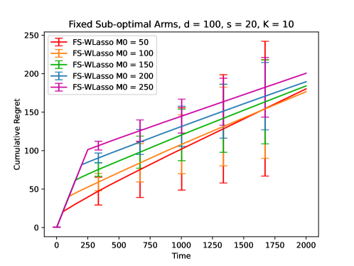
Figure 3: The evaluations of FS-WLasso with various length of forced-sampling stage under the setting of Experiment 2

Furthermore, we even show that $M_{0}=0$ (hence, there is no need to specify it) is a valid choice under more regularity in context distribution in Theorem 2. We believe that this fact provides theoretical evidence that it may not be necessary to choose $M_{0}$ exactly as in Theorem 1 and can be tuned. Again, to be fair, many existing Lasso bandit algorithms also have hyper-parameters that depend on various problem parameters.

Appendix H Auxiliary Lemmas

Lemma 28 (Corollary 6.8 in (Bühlmann and Van De Geer, 2011)).

Let $\boldsymbol{\Sigma}_{0},\boldsymbol{\Sigma}_{1}\in\mathbb{R}^{d\times d}$. Suppose that the compatibility constant of $\boldsymbol{\Sigma}_{0}$ over the index set $S$ with cardinality $s=|S|$ is positive, i.e., $\phi^{2}(\boldsymbol{\Sigma}_{0},S)>0$. If $\|\boldsymbol{\Sigma}_{0}-\boldsymbol{\Sigma}_{1}\|_{\infty}\leq\frac{\phi^{2}(\boldsymbol{\Sigma}_{0},S)}{32s_{0}}$, then $\phi^{2}(\boldsymbol{\Sigma}_{1},S)\geq\phi^{2}(\boldsymbol{\Sigma}_{0},S_{0})/2$.

Lemma 29 (Transfer principle, Lemma 5.1 in (Oliveira, 2016)).

Suppose $\hat{\boldsymbol{\Sigma}}$ and $\bar{\boldsymbol{\Sigma}}$ are $d\times d$ matrices with non-negative diagonal entries. Assume $\eta\in(0,1)$ and $m\in[d]$ are such that

$$\forall\mathbf{v}\in\mathbb{R}^{d}\text{with}\left\|\mathbf{v}\right\|_{0}\leq m,\mathbf{v}^{\top}\hat{\boldsymbol{\Sigma}}\mathbf{v}\geq(1-\eta)\mathbf{v}^{\top}\bar{\boldsymbol{\Sigma}}\mathbf{v}\,.$$

Assume $\mathbf{D}$ is a diagonal matrix whose elements are non-negative and satisfies $\mathbf{D}_{jj}\geq\hat{\boldsymbol{\Sigma}}_{jj}-(1-\eta)\bar{\boldsymbol{\Sigma}}_{jj}$. Then,

$$\forall\mathbf{v}\in\mathbb{R}^{d},\left\|\mathbf{v}\right\|_{0}\leq m,\mathbf{v}^{\top}\hat{\boldsymbol{\Sigma}}\mathbf{v}\geq(1-\eta)\mathbf{v}^{\top}\bar{\boldsymbol{\Sigma}}\mathbf{v}-\frac{\left\|\mathbf{D}\mathbf{v}\right\|_{1}^{2}}{m-1}\,.$$

References

- Abbasi-Yadkori et al. (2011) Y. Abbasi-Yadkori, D. Pál, and C. Szepesvári. Improved algorithms for linear stochastic bandits. Advances in neural information processing systems, 24:2312–2320, 2011.
- Abbasi-Yadkori et al. (2012) Y. Abbasi-Yadkori, D. Pal, and C. Szepesvari. Online-to-confidence-set conversions and application to sparse stochastic bandits. In Artificial Intelligence and Statistics, pages 1–9. PMLR, 2012.
- Abe and Long (1999) N. Abe and P. M. Long. Associative reinforcement learning using linear probabilistic concepts. In International Conference on Machine Learning, pages 3–11, 1999.
- Abeille and Lazaric (2017) M. Abeille and A. Lazaric. Linear Thompson Sampling Revisited. In A. Singh and J. Zhu, editors, Proceedings of the 20th International Conference on Artificial Intelligence and Statistics, volume 54 of Proceedings of Machine Learning Research, pages 176–184. PMLR, PMLR, 20–22 Apr 2017.
- Abeille et al. (2021) M. Abeille, L. Faury, and C. Calauzènes. Instance-wise minimax-optimal algorithms for logistic bandits. In International Conference on Artificial Intelligence and Statistics, pages 3691–3699. PMLR, 2021.
- Agrawal and Goyal (2013) S. Agrawal and N. Goyal. Thompson sampling for contextual bandits with linear payoffs. In International conference on machine learning, pages 127–135. PMLR, 2013.
- Ariu et al. (2022) K. Ariu, K. Abe, and A. Proutière. Thresholded lasso bandit. In International Conference on Machine Learning, pages 878–928. PMLR, 2022.
- Auer (2002) P. Auer. Using confidence bounds for exploitation-exploration trade-offs. Journal of Machine Learning Research, 3(Nov):397–422, 2002.
- Bang and Robins (2005) H. Bang and J. M. Robins. Doubly robust estimation in missing data and causal inference models. Biometrics, 61(4):962–973, 2005.
- Bastani and Bayati (2020) H. Bastani and M. Bayati. Online decision making with high-dimensional covariates. Operations Research, 68(1):276–294, 2020.
- Bastani et al. (2021) H. Bastani, M. Bayati, and K. Khosravi. Mostly exploration-free algorithms for contextual bandits. Management Science, 67(3):1329–1349, 2021.
- Beygelzimer et al. (2011) A. Beygelzimer, J. Langford, L. Li, L. Reyzin, and R. Schapire. Contextual bandit algorithms with supervised learning guarantees. In Proceedings of the Fourteenth International Conference on Artificial Intelligence and Statistics, pages 19–26. JMLR Workshop and Conference Proceedings, 2011.
- Bühlmann and Van De Geer (2011) P. Bühlmann and S. Van De Geer. Statistics for high-dimensional data: methods, theory and applications. Springer Science & Business Media, 2011.
- Castillo et al. (2015) I. Castillo, J. Schmidt-Hieber, and A. Van der Vaart. Bayesian linear regression with sparse priors. The Annals of Statistics, 2015.
- Chakraborty et al. (2023) S. Chakraborty, S. Roy, and A. Tewari. Thompson sampling for high-dimensional sparse linear contextual bandits. In International Conference on Machine Learning, pages 3979–4008. PMLR, 2023.
- Chen et al. (2022) Y. Chen, Y. Wang, E. X. Fang, Z. Wang, and R. Li. Nearly dimension-independent sparse linear bandit over small action spaces via best subset selection. Journal of the American Statistical Association, pages 1–13, 2022.
- Chu et al. (2011) W. Chu, L. Li, L. Reyzin, and R. Schapire. Contextual bandits with linear payoff functions. In Proceedings of the Fourteenth International Conference on Artificial Intelligence and Statistics, pages 208–214. JMLR Workshop and Conference Proceedings, 2011.
- Dani et al. (2008) V. Dani, T. P. Hayes, and S. M. Kakade. Stochastic linear optimization under bandit feedback. In Annual Conference Computational Learning Theory, 2008.
- Faury et al. (2020) L. Faury, M. Abeille, C. Calauzènes, and O. Fercoq. Improved optimistic algorithms for logistic bandits. In International Conference on Machine Learning, pages 3052–3060. PMLR, 2020.
- Faury et al. (2022) L. Faury, M. Abeille, K.-S. Jun, and C. Calauzènes. Jointly efficient and optimal algorithms for logistic bandits. In International Conference on Artificial Intelligence and Statistics, pages 546–580. PMLR, 2022.
- Filippi et al. (2010) S. Filippi, O. Cappé, A. Garivier, and C. Szepesvári. Parametric bandits: The generalized linear case. In Proceedings of the 23rd International Conference on Neural Information Processing Systems - Volume 1, NIPS’10, page 586–594, Red Hook, NY, USA, 2010. Curran Associates Inc.
- Garivier (2013) A. Garivier. Informational confidence bounds for self-normalized averages and applications. In 2013 IEEE Information Theory Workshop (ITW), pages 1–5. IEEE, 2013.
- Gilton and Willett (2017) D. Gilton and R. Willett. Sparse linear contextual bandits via relevance vector machines. In 2017 International Conference on Sampling Theory and Applications (SampTA), pages 518–522. IEEE, 2017.
- Goldenshluger and Zeevi (2013) A. Goldenshluger and A. Zeevi. A linear response bandit problem. Stochastic Systems, 3(1):230–261, 2013.
- Hao et al. (2020a) B. Hao, T. Lattimore, and C. Szepesvari. Adaptive exploration in linear contextual bandit. In International Conference on Artificial Intelligence and Statistics, pages 3536–3545. PMLR, 2020a.
- Hao et al. (2020b) B. Hao, T. Lattimore, and M. Wang. High-dimensional sparse linear bandits. Advances in Neural Information Processing Systems, 33:10753–10763, 2020b.
- Kim and Paik (2019) G.-S. Kim and M. C. Paik. Doubly-robust lasso bandit. Advances in Neural Information Processing Systems, 32, 2019.
- Kveton et al. (2020a) B. Kveton, C. Szepesvári, M. Ghavamzadeh, and C. Boutilier. Perturbed-history exploration in stochastic linear bandits. In Uncertainty in Artificial Intelligence, pages 530–540. PMLR, 2020a.
- Kveton et al. (2020b) B. Kveton, M. Zaheer, C. Szepesvari, L. Li, M. Ghavamzadeh, and C. Boutilier. Randomized exploration in generalized linear bandits. In International Conference on Artificial Intelligence and Statistics, pages 2066–2076. PMLR, 2020b.
- Lai and Robbins (1985) T. L. Lai and H. Robbins. Asymptotically efficient adaptive allocation rules. Advances in applied mathematics, 6(1):4–22, 1985.
- Lattimore and Szepesvári (2020) T. Lattimore and C. Szepesvári. Bandit algorithms. Cambridge University Press, 2020.
- Li et al. (2021) K. Li, Y. Yang, and N. N. Narisetty. Regret lower bound and optimal algorithm for high-dimensional contextual linear bandit. Electronic Journal of Statistics, 15(2):5652–5695, 2021.
- Li et al. (2017) L. Li, Y. Lu, and D. Zhou. Provably optimal algorithms for generalized linear contextual bandits. In International Conference on Machine Learning, pages 2071–2080. PMLR, 2017.
- Li et al. (2016) S. Li, A. Karatzoglou, and C. Gentile. Collaborative filtering bandits. In Proceedings of the 39th International ACM SIGIR conference on Research and Development in Information Retrieval, pages 539–548, 2016.
- Li et al. (2022) W. Li, A. Barik, and J. Honorio. A simple unified framework for high dimensional bandit problems. In International Conference on Machine Learning, pages 12619–12655. PMLR, 2022.
- Oh et al. (2021) M.-h. Oh, G. Iyengar, and A. Zeevi. Sparsity-agnostic lasso bandit. In International Conference on Machine Learning, pages 8271–8280. PMLR, 2021.
- Oliveira (2016) R. I. Oliveira. The lower tail of random quadratic forms with applications to ordinary least squares. Probability Theory and Related Fields, 166:1175–1194, 2016.
- Papini et al. (2021) M. Papini, A. Tirinzoni, M. Restelli, A. Lazaric, and M. Pirotta. Leveraging good representations in linear contextual bandits. In International Conference on Machine Learning, pages 8371–8380. PMLR, 2021.
- Robbins (1952) H. Robbins. Some aspects of the sequential design of experiments. Bulletin of the American Mathematical Society, 1952.
- Rusmevichientong and Tsitsiklis (2010) P. Rusmevichientong and J. N. Tsitsiklis. Linearly parameterized bandits. Mathematics of Operations Research, 35(2):395–411, 2010.
- Tewari and Murphy (2017) A. Tewari and S. A. Murphy. From ads to interventions: Contextual bandits in mobile health. Mobile health: sensors, analytic methods, and applications, pages 495–517, 2017.
- Tibshirani (1996) R. Tibshirani. Regression shrinkage and selection via the lasso. Journal of the Royal Statistical Society Series B: Statistical Methodology, 58(1):267–288, 1996.
- Van De Geer and Bühlmann (2009) S. A. Van De Geer and P. Bühlmann. On the conditions used to prove oracle results for the lasso. Electronic Journal of Statistics, 2009.
- Wang et al. (2018) X. Wang, M. Wei, and T. Yao. Minimax concave penalized multi-armed bandit model with high-dimensional covariates. In International Conference on Machine Learning, pages 5200–5208. PMLR, 2018.
- Zeng et al. (2016) C. Zeng, Q. Wang, S. Mokhtari, and T. Li. Online context-aware recommendation with time varying multi-armed bandit. In Proceedings of the 22nd ACM SIGKDD international conference on Knowledge discovery and data mining, pages 2025–2034, 2016.
- Zhang (2010) C.-H. Zhang. Nearly unbiased variable selection under minimax concave penalty. The Annals of Statistics, 2010.
- Zhou (2010) S. Zhou. Thresholded lasso for high dimensional variable selection and statistical estimation. arXiv preprint arXiv:1002.1583, 2010.