Learning-Based Verification of Stochastic Dynamical Systems with Neural Network Policies

Abstract

We consider the verification of neural network policies for reach-avoid control tasks in stochastic dynamical systems. We use a verification procedure that trains another neural network, which acts as a certificate proving that the policy satisfies the task. For reach-avoid tasks, it suffices to show that this certificate network is a reach-avoid supermartingale (RASM). As our main contribution, we significantly accelerate algorithmic approaches for verifying that a neural network is indeed a RASM. The main bottleneck of these approaches is the discretization of the state space of the dynamical system. The following two key contributions allow us to use a coarser discretization than existing approaches. First, we present a novel and fast method to compute tight upper bounds on Lipschitz constants of neural networks based on weighted norms. We further improve these bounds on Lipschitz constants based on the characteristics of the certificate network. Second, we integrate an efficient local refinement scheme that dynamically refines the state space discretization where necessary. Our empirical evaluation shows the effectiveness of our approach for verifying neural network policies in several benchmarks and trained with different reinforcement learning algorithms.

1 Introduction

Feed-forward neural networks are widely used in reinforcement learning (RL) to represent policies in challenging control problems [48, 56, 30]. These problems involve continuous, non-linear, and stochastic dynamics and are thus commonly modeled as stochastic dynamical systems [21]. Despite showing impressive potential, common RL algorithms generally do not provide formal guarantees about produced policies. This lack of guarantees prevents the deployment of neural network policies to safety-critical domains, where guarantees on system behavior are imperative [10]. The desired behavior of these systems can often be expressed as a (probabilistic) reach-avoid specification, which is a triple of goal states, unsafe states, and a threshold probability [62]. Intuitively, a (neural network) policy deployed on a dynamical system satisfies a reach-avoid specification, if the probability of reaching the goal states without visiting the unsafe states is above the required threshold. In this paper, we study the following specific problem: Given a (known) discrete-time non-linear stochastic system and a neural network policy, verify whether the policy satisfies a given reach-avoid specification.

We address this problem by finding a certificate that proves the satisfaction of the reach-avoid specification. To find such a certificate, we build upon popular inductive synthesis methods and use the learner-verifier framework shown in Fig. 1. Given an input policy, this framework alternates between a learner that learns a candidate certificate and a verifier that attempts to verify the validity of the certificate. The verifier either proves the validity of the certificate or returns counterexamples (or more general diagnostic information) to guide the learner to improve the candidate. Importantly, the termination of the framework proves that the policy satisfies the specification.

In non-stochastic control, Lyapunov functions are the classical certificate to prove the stability of dynamical systems [42]. Intuitively, Lyapunov methods reduce the problem of certifying behavior over paths to verifying that a scalar certificate function (interpreted as the system’s energy level) decreases with every step under the dynamics. For stochastic systems, as we consider, this certificate function must decrease at every step under the dynamics in expectation, i.e., needs to be a supermartingale [67, 53]. Such martingale-based certificates are a natural framework for certifying stochastic systems and have recently been used for stochastic reach-avoid control by [73]. Their certificates, called reach-avoid supermartingales (RASM), are represented as (feed-forward) neural networks and fit naturally in the learner-verifier framework in Fig. 1.

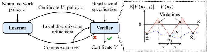
Figure 1: Our learner-verifier framework for verifying neural network policies. To verify the validity of the candidate RASM $V$, we must show that $V$ decreases strictly in expectation for all states $\mathbf{x}$ (i.e., the blue line is strictly below zero). The verifier uses a discretization with mesh size $\tau$ and an upper bound $K$ on the Lipschitz constant to upper bound the expected decrease (shown by the red line). The current upper bound violates the required condition, which can be fixed by decreasing $\tau$ or $K$.

The main challenge in verifying the validity of a candidate RASM is to show that, from every state, the RASM decreases in expectation with the one-step dynamics. This expected decrease condition is shown by the blue line in Fig. 1, so we must show that this line is strictly negative in every state $\mathbf{x}$. However, due to the continuity of the system, checking this condition at every state is infeasible. Thus, existing approaches check stronger conditions on a discretization of the state space (points $\tilde{\mathbf{x}}_{1},\tilde{\mathbf{x}}_{2},\tilde{\mathbf{x}}_{3}$ in Fig. 1) and use Lipschitz continuity of the policy and the RASM to show that the conditions hold on the entire state space. However, this analysis is computationally expensive and leads to very conservative results in practice. First, computing the (smallest) Lipschitz constant of a neural network exactly is intractable [65], so existing approaches use (loose) upper bounds instead. Second, reducing the mesh size $\tau$ may result in having to check the conditions at prohibitively many points.

In this work, we present an effective verifier for RASMs that addresses both of the challenges above. Our approach combines two key features: (1) an efficient method for computing tight upper bounds on Lipschitz constants for neural networks, and (2) a local discretization refinement scheme. A novel aspect of our method to compute bounds on Lipschitz constants is that we use weighted norm systems. To the best of our knowledge, weighted norms have not been used before to compute Lipschitz constants of neural networks. In combination with averaged activation operators [27], our method leads to significantly tighter global bounds on Lipschitz constants for neural networks. Furthermore, we locally improve these bounds using the characteristics of the output activation function of the RASM. The second key aspect of our approach is a local refinement scheme that only refines the discretization at points where necessary. Critically, whenever a discretized point violates the RASM conditions, we can determine if the violation could be mitigated by further refining that point. Following this intuition, we present an algorithm that locally refines the discretization while avoiding unnecessary computations in cases where refinement cannot fix violations.

Contributions    In summary, we present an effective verifier of neural network policies for non-linear stochastic systems with reach-avoid specifications. Our approach combines a method to compute better bounds on Lipschitz constants with a local discretization refinement scheme. Our thorough empirical evaluation shows the effectiveness of our approach in both existing and new benchmarks and with neural network policies trained with different RL algorithms. We are able to verify reach-avoid specifications with higher probability bounds and at lower run times than the state-of-the-art.

Related Work

Loosely related are constrained [5, 8] and safe RL [14, 7], which compute policies, often in unknown dynamics, and with (besides maximizing rewards) constraints on expected costs, or on safety in exploration. We refer to surveys [19, 33] for details. Our setting is different: we consider systems with known dynamics and provide formal guarantees on a given neural network policy. Another approach to stochastic control with known dynamics is to generate a finite abstraction as a Markov decision process (MDP) [70, 45, 12]. These methods can handle rich specifications [46], but abstractions easily get prohibitively large, and verifying neural network policies on these abstractions is challenging.

Certificate functions    Lyapunov [42, 29] and control barrier functions [9, 69, 49, 25] are certificate functions widely used to verify stability and safety of dynamical systems, respectively. Variants for stochastic systems have been studied by, e.g., [53, 26, 51, 39], but have received less attention. To show the validity of a stochastic Lyapunov or barrier function, one must typically show that its expected value is (strictly) decreasing under the system dynamics [53], i.e., yields a supermartingale [67]. Supermartingales are also used to analyze termination [22, 6, 24, 3] and reachability [64] of probabilistic programs. Standard approaches to finding certificate functions mostly use (convex) optimization over a fixed template, such as exponential functions [61] or low-degree sum-of-squares (SoS) polynomials [58]. As these templates are often too restrictive, various recent papers represent certificates as neural networks [23, 2, 57, 72, 68] (called neural certificates [28]). Generally speaking, the neural network is trained on a differentiable version of the conditions the certificate must satisfy, e.g., decreasing in expectation. The resulting candidate certificate (i.e., the neural network) can be verified using satisfiability modulo theories (SMT) [4, 1], branch-and-bound [50], or discretization and leveraging Lipschitz constants [73, 47]. Our approach relates to the latter category and, in particular, the martingale-based certificate for reach-avoid specifications proposed by [73, 74].

Neural network robustness    The use of Lipschitz constants as a measure of neural network stability and robustness was pioneered by [63], who propose the product of the Lipschitz constants of each layer as an upper bound for the Lipschitz constant of the network. Methods for computing local Lipschitz constants include [66, 71, 40, 34, 60, 11]. Algorithms that compute the global Lipschitz constant of a network include [32, 16]. However, these methods are generally expensive and thus unsuitable in our context, because we need to compute Lipschitz constants multiple times in each learner-verifier iteration. Combettes and Pesquet [27] exploit the fact that many activation functions, including the ReLU, can be written as the average of the identity function and a function with Lipschitz constant 1. Here, we combine the method from [27] with a novel method. Besides approaches to bound Lipschitz constants, training networks to have a small Lipschitz constant is studied by [20, 35, 52]. However, for our purposes, we need a (tight) upper bound of the Lipschitz constant. Another approach to neural network robustness is interval bound propagation (IBP), a technique to propagate interval inputs through neural networks [36]. IBP generally leads to tighter bounds than Lipschitz constants but is not applicable to all RASM conditions we need to verify. Finally, a different line of research considers the adversarial robustness of neural networks [17, 63, 44, 37, 41]. For a more comprehensive overview of verification and robustness of neural networks, we refer to the surveys [38, 75].

2 Problem Statement

Stochastic dynamical system    Consider a discrete-time, stochastic (non-linear) dynamical system where the state space variable $\mathbf{x}_{t}\in\mathcal{X}\subseteq\mathbb{R}^{d}$ evolves over discrete time steps $t\in\mathbb{N}_{0}$ as

$$\mathbf{x}_{t+1}=f(\mathbf{x}_{t},\mathbf{u}_{t},\omega_{t}),\quad\mathbf{x}_{0}\in\mathcal{X}_{0},\quad\omega_{t}\sim\mu$$ (1)

where $\mathcal{X}_{0}\subseteq\mathcal{X}$ is a set of initial states, $\mathbf{u}_{t}\in\mathcal{U}\subseteq\mathbb{R}^{m}$ is the control input, and $\omega_{t}\in\mathcal{N}\subseteq\mathbb{R}^{p}$ is a stochastic disturbance, defined on a probability space $(\mathcal{N},\mathcal{B}_{\mathcal{N}},\mu)$ with the Borel $\sigma$-algebra $\mathcal{B}_{\mathcal{N}}$ on $\mathcal{N}$ and probability measure $\mu\colon\mathcal{B}_{\mathcal{N}}\to[0,1]$ (see, e.g., [31] for details). The system dynamics are defined by the function $f\colon\mathcal{X}\times\mathcal{U}\times\mathcal{N}\to\mathcal{X}$. An execution of the stochastic dynamical system is an infinite sequence $(\mathbf{x}_{t},\mathbf{u}_{t},\omega_{t})_{t\in\mathbb{N}_{0}}$ of state-action-disturbance triples, such that for all $t\in\mathbb{N}_{0}$, we have $\mathbf{x}_{t+1}=f(\mathbf{x}_{t},\mathbf{u}_{t},\omega_{t})$, $\mathbf{u}_{t}\in\mathcal{U}$, and $\omega_{t}\in\mathsf{support}(\mu)$.

Policy    A policy $\pi\colon\mathcal{X}\to\mathcal{U}$ chooses the control inputs such that $\mathbf{u}_{t}\coloneqq\pi(\mathbf{x}_{t})$ in Eq. 1. Here, we assume that the policy $\pi$ is represented as a neural network. Fixing a policy $\pi$ and an initial state $\mathbf{x}_{0}\in\mathcal{X}_{0}$ defines a Markov process in the probability space of all executions [15, 54]. We denote the probability measure and the expectation in this probability space by $\mathbb{P}^{\pi}_{\mathbf{x}_{0}}$ and $\mathbb{E}^{\pi}_{\mathbf{x}_{0}}$, respectively.

Reach-avoid specification    For the Markov process defined by a policy $\pi$ and initial state $\mathbf{x}_{0}\in\mathcal{X}_{0}$ for the system in Eq. 1, we want to evaluate the probability of reaching a target set $\mathcal{X}_{T}\subseteq\mathcal{X}$ before reaching an unsafe set $\mathcal{X}_{U}\subseteq\mathcal{X}$. Formally, this reach-avoid probability $\mathrm{Pr}^{\pi}_{\mathbf{x}_{0}}(\mathcal{X}_{T},\mathcal{X}_{U})$ is defined as

$$\mathrm{Pr}^{\pi}_{\mathbf{x}_{0}}(\mathcal{X}_{T},\mathcal{X}_{U})\coloneqq\mathbb{P}^{\pi}_{\mathbf{x}_{0}}\big{\{}\exists t\in\mathbb{N}_{0}\,:\,\mathbf{x}_{t}\in\mathcal{X}_{T}\wedge(\forall t^{\prime}\in\{0,\ldots,t\}:\mathbf{x}_{t^{\prime}}\notin\mathcal{X}_{U})\big{\}}.$$ (2)

Intuitively, $\mathrm{Pr}^{\pi}_{\mathbf{x}_{0}}(\mathcal{X}_{T},\mathcal{X}_{U})$ is the probability that, from initial state $\mathbf{x}_{0}$, the system eventually reaches $\mathcal{X}_{T}$ while never reaching $\mathcal{X}_{U}$ before. A reach-avoid specification is a triple $(\mathcal{X}_{T},\mathcal{X}_{U},\rho)$ and is satisfied if $\mathrm{Pr}^{\pi}_{\mathbf{x}_{0}}(\mathcal{X}_{T},\mathcal{X}_{U})\geq\rho$ for all $\mathbf{x}_{0}\in\mathcal{X}_{0}$. We state the formal problem that we solve.

Problem 1.

Given a policy $\pi$ for the stochastic dynamical system in Eq. 1, verify whether the reach-avoid specification $(\mathcal{X}_{T},\mathcal{X}_{U},\rho)$ is satisfied, i.e., $\mathrm{Pr}^{\pi}_{\mathbf{x}_{0}}(\mathcal{X}_{T},\mathcal{X}_{U})\geq\rho\,$ for all $\mathbf{x}_{0}\in\mathcal{X}_{0}$.

In solving this problem, we make the following assumptions, which are very general and standard in, e.g., control theory. These assumptions ensure that the reach-avoid probability is well-defined [15].

Assumption 1.

(1) The transition function $f$ and the policy $\pi$ are Lipschitz continuous; (2) The sets $\mathcal{X}$, $\mathcal{X}_{0}$, $\mathcal{X}_{T}$, $\mathcal{X}_{U}$ and $\mathcal{U}$ are Borel-measurable; (3) $\mathcal{X}$ and $\mathcal{N}$ are compact (i.e., closed and bounded).

3 Verifying Reach-Avoid Specifications using Supermartingales

In this section, we fix a stochastic dynamical system as in Eq. 1, a policy $\pi$, and a reach-avoid specification $(\mathcal{X}_{T},\mathcal{X}_{U},\rho)$. We recap the certificate, called a reach-avoid supermartingale (RASM), and the verification procedure, proposed by Zikelic et al. [73] to provide reach-avoid guarantees.

Definition 1 (Reach-avoid supermartingale).

A continuous function $V\colon\mathcal{X}\to\mathbb{R}_{\geq 0}$ is a reach-avoid supermartingale (RASM) if the following hold: (1) Initial condition: $V(\mathbf{x})\leq 1$ for all $\mathbf{x}\in\mathcal{X}_{0}$; and (2) Safety condition: $V(\mathbf{x})\geq\frac{1}{1-\rho}$ for all $\mathbf{x}\in\mathcal{X}_{U}$; and (3) Expected decrease condition: There exists $\epsilon>0$ such that $\mathbb{E}_{\omega\sim\mu}\left[V(f(\mathbf{x},\pi(\mathbf{x}),\omega))\right]\leq V(\mathbf{x})-\epsilon$ for each $\mathbf{x}\in\mathcal{X}\setminus\mathcal{X}_{T}$ with $V(\mathbf{x})\leq\frac{1}{1-\rho}$.

A RASM associates each state with a non-negative value and decreases in expectation with at least $\epsilon$ at every step in the dynamics. To reach an unsafe state from any initial state, the value of the RASM $V(\mathbf{x}_{k})$ needs to increase from at most 1 to at least $\frac{1}{1-\rho}$ along the execution, which happens with probability at most $1-\rho$, since $V$ decreases in expectation with every step along the execution. The existence of a RASM implies that the reach-avoid specification in Problem 1 is satisfied:

Theorem 1 ([73], proof in Sect. B.2).

If there exists a RASM, then the reach-avoid specification is satisfied.

Representation of $V$    In this work, we represent RASM candidates, i.e., functions of the form $V\colon\mathcal{X}\to\mathbb{R}_{\geq 0}$, as neural networks. We use a Softplus output activation function to ensure the non-negativity requirement. We then embed the candidate RASM in the learner-verifier framework as in Fig. 1. In each iteration, the verifier checks whether the candidate RASM proposed by the learner is a RASM by checking a set of (slightly stronger) conditions that we define below in Def. 3.

Discretization    Since the state space $\mathcal{X}$ is continuous, it is not feasible to check the conditions from Def. 1 on each point $\mathbf{x}\in\mathcal{X}$ separately. Instead, we check slightly stronger versions of the conditions from Def. 1 on a discretization of the state space into rectangular cells. Concretely, for a given mesh size $\tau>0$, define $\mathrm{cell}^{\tau}_{\infty}(\mathbf{x})=\{\mathbf{x}^{\prime}:\|\mathbf{x}-\mathbf{x}^{\prime}\|_{\infty}\leq\tau/d\}$, where $\|\cdot\|_{\infty}$ denotes the $\infty$-norm. Dividing by $d$ in the definition of $\mathrm{cell}^{\tau}_{\infty}(\mathbf{x})$ ensures that $\|\mathbf{x}-\mathbf{x}^{\prime}\|_{1}\leq\tau$ for all $\mathbf{x}^{\prime}\in\mathrm{cell}^{\tau}_{\infty}(\mathbf{x})$ (which we need later in Def. 3). We define the following discretization of $\mathcal{X}$.

Definition 2 (Discretization of $\mathcal{X}$).

Let $\tau>0$ be a mesh size. A finite set of points $\widetilde{\mathcal{X}}$ is a discretization of $\mathcal{X}$ if for every $\mathbf{x}\in\mathcal{X}$ there exists an $\tilde{\mathbf{x}}\in\widetilde{\mathcal{X}}$ such that $\mathbf{x}\in\mathrm{cell}_{\infty}^{\tau}(\tilde{\mathbf{x}})$.

Conditions on the discretization    We define a stronger version of the RASM conditions, such that the satisfaction of these stronger conditions on each point $\tilde{\mathbf{x}}\in\widetilde{\mathcal{X}}$ from a discretization of $\mathcal{X}$ implies the satisfaction of the conditions in Def. 1. Toward these stronger conditions, we define

$$V_{\mathrm{min}}(\tilde{\mathbf{x}})=\min\limits_{\mathbf{x}\in\mathrm{cell}^{\tau}_{\infty}(\tilde{\mathbf{x}})}V(\mathbf{x})\qquad\text{and}\qquad V_{\mathrm{max}}(\tilde{\mathbf{x}})=\max\limits_{\mathbf{x}\in\mathrm{cell}^{\tau}_{\infty}(\tilde{\mathbf{x}})}V(\mathbf{x})$$

as the min/max of $V$ within each cell $\mathrm{cell}^{\tau}_{\infty}(\tilde{\mathbf{x}})$, $\tilde{\mathbf{x}}\in\widetilde{\mathcal{X}}$. Computing $V_{\mathrm{min}}(\mathbf{x})$ and $V_{\mathrm{max}}(\mathbf{x})$ analytically is in general not possible, but using interval bound propagation (IBP) [36] we can compute bounds $V_{\mathrm{LB}}(\mathbf{x})$ and $V_{\mathrm{UB}}(\mathbf{x})$ satisfying $V_{\mathrm{LB}}(\mathbf{x})\leq V_{\mathrm{min}}(\mathbf{x})\leq V(\mathbf{x})\leq V_{\mathrm{max}}(\mathbf{x})\leq V_{\mathrm{UB}}(\mathbf{x})$. These bounds obtained from IBP are generally tighter than those computed using Lipschitz constants.

Besides IBP, we also use Lipschitz continuity (using 1-norms). We say that $L_{g}$ is a Lipschitz constant of a function $g$ if $\|g(x)-g(x^{\prime})\|_{1}\leq L_{g}\|x-x^{\prime}\|_{1}$ for all $x,x^{\prime}$ in the domain of $g$. All Lipschitz constants that we discuss in this paper will be with respect to the 1-norm. Let $L_{f}$ and $L_{\pi}$ be Lipschitz constants of the dynamics $f$ and the policy $\pi$, respectively.

Concretely, the satisfaction of the conditions in Def. 1 is then implied by the following conditions.

Definition 3 (Discrete RASM).

Let $V\colon\mathcal{X}\to\mathbb{R}_{\geq 0}$ be Lipschitz continuous with Lipschitz constant $L_{V}$. Define $K=L_{V}L_{f}\left(L_{\pi}+1\right)$ and let $\widetilde{\mathcal{X}}$ be a discretization with mesh size $\tau$. Then, $V$ is a discrete RASM for $\widetilde{\mathcal{X}}$ if the following hold: (1) Initial condition: $V_{\mathrm{UB}}(\tilde{\mathbf{x}})\leq 1$ for all $\tilde{\mathbf{x}}\in\widetilde{\mathcal{X}}$ such that $\mathrm{cell}_{\infty}^{\tau}(\tilde{\mathbf{x}})\cap\mathcal{X}_{0}\neq\emptyset$; and (2) Safety condition: $V_{\mathrm{LB}}(\tilde{\mathbf{x}})\geq\frac{1}{1-\rho}$ for all $\tilde{\mathbf{x}}\in\widetilde{\mathcal{X}}$ such that $\mathrm{cell}_{\infty}^{\tau}(\tilde{\mathbf{x}})\cap\mathcal{X}_{U}\neq\emptyset$; and (3) Expected decrease condition:

$$\mathbb{E}_{\omega\sim\mu}\left[V(f(\tilde{\mathbf{x}},\pi(\tilde{\mathbf{x}}),\omega))\right]<V_{\mathrm{LB}}(\tilde{\mathbf{x}})-\tau K$$ (3)

for all $\tilde{\mathbf{x}}\in\widetilde{\mathcal{X}}$ such that $\mathrm{cell}_{\infty}^{\tau}(\tilde{\mathbf{x}})\cap(\mathcal{X}\setminus\mathcal{X}_{T})\neq\emptyset$ and $V_{\mathrm{LB}}(\tilde{\mathbf{x}})<\frac{1}{1-\rho}$.

We deviate slightly from [73], which instead uses $V(\tilde{\mathbf{x}})-\tau(K+L_{V})$ on the right-hand side of Eq. 3. Since IBP usually gives tighter bounds than Lipschitz continuity, our version of Eq. 3 is (slightly) easier to satisfy. Verifying the conditions in Def. 3 is sufficient to show that $V$ is a RASM:

Lemma 1 (proof in Sect. B.3).

If $V$ is a discrete RASM for a discretization $\widetilde{\mathcal{X}}$, then $V$ is a RASM.

Exactly computing the expected value in Eq. 3 is generally infeasible. Thus, we instead bound this expectation from above by discretizing the noise space $\mathcal{N}$ into a collection of cells $\mathcal{C}$, such that $\mathbb{E}_{\omega\sim\mu}\left[V(f(\tilde{\mathbf{x}},\pi(\tilde{\mathbf{x}}),\omega))\right]\leq\sum_{C\in\mathcal{C}}\mathbb{P}(\omega\in C)\sup_{\omega\in C}\left[V(f(\tilde{\mathbf{x}},\pi(\tilde{\mathbf{x}}),\omega))\right],$ where in practice, we again use IBP to upper bound $\sup_{\omega\in C}\left[V(f(\tilde{\mathbf{x}},\pi(\tilde{\mathbf{x}}),\omega))\right]$ for each cell $C\in\mathcal{C}$.

Challenges    The existing verification procedure based on the discrete RASM conditions in Def. 3 is generally conservative and computationally expensive. The scalability of the procedure is especially limited by the double discretization (for both the state space and the noise space). Furthermore, the tightness of the constraint in Eq. 3 depends on (1) the Lipschitz constant $K$, for which we can only compute (conservative) upper bounds in practice, and (2) the mesh size $\tau$. In Sect. 4, we present our method to compute better upper bounds on Lipschitz constants for neural networks, and in Sect. 5 our local refinement scheme that reduces the number of points needed in the discretization.

4 Lipschitz Constants of Neural Networks

We present our main theoretical contribution, which is a novel method to compute tighter Lipschitz constants for feed-forward neural networks. First, to obtain tighter global Lipschitz constants, we combine the use of weighted 1-norms defined by $\|x\|=\sum_{i}w_{i}\lvert x_{i}\rvert$ (for weights $w_{i}>0$) with averaged activation operators [27]. Second, we locally improve these global Lipschitz constants using the characteristics of the Softplus activation function in the output layer of $V$.

Definition 4.

An $(n+1)$-layer (feed-forward) neural network with dimensions $m_{k}$ ($0\leq k\leq n$) consists of the matrices $A_{k}\in\mathbb{R}^{m_{k}\times m_{k-1}}$, the biases $b_{k}\in\mathbb{R}^{m_{k}}$, and the activation functions $R_{k}\colon\mathbb{R}^{m_{k}}\to\mathbb{R}^{m_{k}}$ ($1\leq k\leq n$). The operator $T\colon\mathbb{R}^{m_{0}}\to\mathbb{R}^{m_{n}}$ corresponding to the neural network maps $x_{0}$ to $x_{n}$, where for $1\leq k\leq n$, $x_{k}$ is defined recursively by $x_{k}=R_{k}\left(A_{k}x_{k-1}+b_{k}\right)$.

We restrict ourselves to activation functions with Lipschitz constant 1, which includes the most commonly used activation functions such as ReLU, Softplus, tanh, and sigmoid. In the following, we use the notation introduced in Def. 4 for the components of the neural network.

4.1 Weighted Norms

We first introduce weight systems, which consist of a weighted $1$-norm for each layer of the network.

Definition 5.

A weight system $\mathcal{W}$ for an $(n\!+\!1)$-layer neural network consists of a weighted 1-norm $\|x\|_{\mathcal{W}}^{k}=\sum_{i=1}^{m_{k}}w_{i}^{k}|x_{i}|$ for each layer $0\leq k\leq n$, where $w^{k}\in\mathbb{R}_{>0}^{m_{k}}$ and $\max_{i}w_{i}^{k}=1$. We define the Lipschitz bound for a weight system $\mathcal{W}$ as $L_{T,\mathcal{W}}=\prod_{\ell=1}^{n}\!\|A_{\ell}\|^{\ell-1,\ell}_{\mathcal{W}}$, where the weighted norm for a matrix $M\in\mathbb{R}^{m_{\ell}\times m_{k}}$ is $\|M\|^{k,\ell}_{\mathcal{W}}=\sup\Big{\{}\frac{\|Mx\|^{\ell}_{\mathcal{W}}}{\|x\|^{k}_{\mathcal{W}}}\!~{}\Big{|}~{}\!x\in\mathbb{R}^{m_{k}},x\neq 0\Big{\}}$.

The Lipschitz bound $L_{T,\mathcal{W}}$ is indeed a Lipschitz constant of the neural network operator $T$:

Lemma 2 (proof in Sect. B.4).

Let $\mathcal{W}$ be a weight system. Then $L_{T,\mathcal{W}}$ is a Lipschitz constant of $T$, i.e. $\|T(x)-T(x^{\prime})\|^{n}_{\mathcal{W}}\leq L_{T,\mathcal{W}}\|x-x^{\prime}\|^{0}_{\mathcal{W}}$ for all $x,x^{\prime}\in\mathbb{R}^{m_{0}}$. In the special case of $w^{n}_{i}=1$ for all $1\leq i\leq m_{n}$, $L_{T,\mathcal{W}}$ is also a Lipschitz constant of $T$ when equipping the input and output space with the standard (unweighted) 1-norm, i.e. $\|T(x)-T(x^{\prime})\|\leq L_{T,\mathcal{W}}\|x-x^{\prime}\|$ for all $x,x^{\prime}\in\mathbb{R}^{m_{0}}$.

For given weights on the final layer, the goal is to compute a weight system $\mathcal{W}$ such that $L_{T,\mathcal{W}}$ is optimal (i.e., lowest) among all weight systems. Observe that the Lipschitz bound decreases when the weights on the input layer increase. This observation motivates the following optimality criterion for weights, which is based on the product of the Lipschitz bound and the weights on the input layer.

Definition 6 (Optimality).

Let $S$ be a set of pairs consisting of input weights $w^{0}$ and a Lipschitz bound $K$. A pair $(w^{0},K)\in S$ is optimal for $S$ if $\widetilde{K}\widetilde{w}^{0}_{j}\geq Kw^{0}_{j}$ for all $1\leq j\leq m_{0}$ and all $(\widetilde{w}^{0},\widetilde{K})\in S$.

Lemma 3 (proof in Sect. B.5).

If $(w^{0},K)$ is optimal for $S$, then $K\leq\widetilde{K}$ for all $(\widetilde{w}^{0},\widetilde{K})\in S$.

We compute optimal $\mathcal{W}$ and $L_{T,\mathcal{W}}$, via the following auxiliary lemma.

Lemma 4 (proof in Sect. B.6).

Let $M\in\mathbb{R}^{m_{\ell}\times m_{k}}$ be a matrix with entries $M_{ij}$. Equip the space $\mathbb{R}^{m_{\ell}}$ with the norm $\|x\|_{\mathcal{W}}^{k}=\sum_{i=1}^{m_{k}}w_{i}^{k}\lvert x_{i}\rvert$, and the space $\mathbb{R}^{m_{k}}$ with the norm $\|x\|_{\mathcal{W}}^{\ell}=\sum_{i=1}^{m_{\ell}}w_{i}^{\ell}\lvert x_{i}\rvert$. Then the corresponding matrix norm satisfies $\|M\|^{k,\ell}_{\mathcal{W}}\;=\;\max\limits_{1\leq j\leq m_{k}}\left[\frac{1}{w_{j}^{k}}\sum_{i=1}^{m_{\ell}}w_{i}^{\ell}\left\lvert M_{ij}\right\rvert\right]$.

Algorithm 1 Computing optimal weights.

Output weights $w^{n}$ for output layer $n$, matrices $A_{k}\in\mathbb{R}^{m_{k}\times m_{k-1}}$ ($1\leq k\leq n$) as in Def. 4.

Input weights $w^{0}$ and a Lipschitz bound $K$ such that $(w^{0},K)$ is optimal.

for $\ell=n,\dots,1$ do

   $K_{\ell}$ $\leftarrow$ $\!\max_{1\leq j\leq m_{\ell-1}}\sum_{i=1}^{m_{\ell}}\!w_{i}^{\ell}\left\lvert(A_{\ell})_{ij}\right\rvert$ $\triangleright$ Lipschitz constant $\|A_{\ell}\|^{\ell-1,\ell}_{\mathcal{W}}$ if $w^{\ell-1}_{j}=1$ for all $j$

   for $j=1,\dots,m_{\ell-1}$ do

      $w_{j}^{\ell-1}$ $\leftarrow$ $\frac{1}{K_{\ell}}\!\sum_{i=1}^{m_{\ell}}\!w_{i}^{\ell}\left\lvert(A_{\ell})_{ij}\right\rvert$$\triangleright$ Smallest weight for which the Lipschitz constant is $K_{\ell}$    return $w^{0}$, $\prod_{\ell=1}^{n}K_{\ell}$ $\triangleright$ Return input weights and Lipschitz bound $K$

Given weights $w^{\ell}_{i}$ for the space $\mathbb{R}^{m_{\ell}}$, we can set the normalized weights $w_{j}^{k}$ proportional to $\sum_{i=1}^{m_{\ell}}w_{i}^{\ell}\left\lvert M_{ij}\right\rvert$, which implies that the maximum in Lemma 4 is attained for all $1\leq j\leq m_{k}$. Algorithm 1 starts from given output weights $w^{n}_{i}$ and iteratively computes weights $w_{j}^{\ell-1}$ given weights $w_{i}^{\ell}$ in this way such that the maximum in Lemma 4 is attained by all $1\leq j\leq m_{\ell-1}$ for the matrix $M=A_{\ell}$. The following theorem shows that Algorithm 1 indeed computes optimal weights.

Theorem 2 (Correctness of Algorithm 1; proof in Sect. B.7).

Let output weights $w^{n}$ be given. The input weights $w^{0}$ and Lipschitz bound $K$ computed using Algorithm 1 are optimal among the set of pairs $(w^{0},L_{T,\mathcal{W}})$ that can be computed by choosing a weight system $\mathcal{W}$.

By choosing the same unweighted norm for each layer, one may recover the Lipschitz bound from [63], which corresponds to the approach presented in [73]. To further tighten the Lipschitz bound, we integrate weighted norms with averaged activation operators [27]. For details, we refer to Sect. A.1.

4.2 Local Lipschitz constants using the Softplus activation function

In Sect. 4.1, we discussed how to compute tighter global Lipschitz constants. We further improve these global Lipschitz constants based on local Lipschitz constants for the Softplus output activation function of the neural network certificate $V$. Let us denote $\widetilde{V}(\mathbf{x})$ as the value of the certificate before applying the Softplus, such that we can write $V(\mathbf{x})=\mathrm{SoftPlus}(\widetilde{V}(\mathbf{x}))$. In Sect. 4.1, we use the global Lipschitz constant of the Softplus (which is 1), resulting in the same Lipschitz constant for both $\widetilde{V}$ and $V$. However, the derivative of the Softplus function, which is a local Lipschitz constant of the Softplus function, is (much) smaller than 1 for small inputs. We can multiply this derivative with the global Lipschitz constant of $\widetilde{V}$ to obtain a (tighter) local Lipschitz constant for $V$.

To satisfy the expected decrease condition in Def. 3 at a point $\tilde{\mathbf{x}}_{t}\in\widetilde{\mathcal{X}}$, we need at least that $\mathbb{E}[V(\tilde{\mathbf{x}}_{t+1})]<V(\tilde{\mathbf{x}}_{t})$. To check this inequality for all $\mathbf{x}_{t}\in\mathrm{cell}_{\infty}^{\tau}(\tilde{\mathbf{x}}_{t})$, we thus need the (expected) local Lipschitz constant at the new state $\tilde{\mathbf{x}}_{t+1}=f(\tilde{\mathbf{x}}_{t},\pi(\tilde{\mathbf{x}}_{t}),\omega)$. Due to $\omega\sim\mu$ being random, we prefer to compute the local Lipschitz constant at $\mathbf{x}_{t}$ instead, which is possible due to the following observation: The local Lipschitz constant (i.e., derivative) $1-e^{-\mathrm{SoftPlus}(\widetilde{V}(\mathbf{x}))}=1-e^{-V(\mathbf{x})}$ of the Softplus is concave and increasing in $V(\mathbf{x})$, which implies that $\mathbb{E}[1-e^{-V(\mathbf{x}_{t+1})}]<1-e^{-\mathbb{E}[V(\mathbf{x}_{t+1})]}<1-e^{-V(\mathbf{x}_{t})}$ by Jensen’s inequality. Hence, the expected local Lipschitz constant at $\widetilde{V}(\mathbf{x}_{t+1})$ is smaller than the local Lipschitz constant at $\widetilde{V}(\mathbf{x})$. This intuition is formalized by Theorem 3.

Theorem 3 (proof in Sect. B.8).

Let $V(\mathbf{x})=\mathrm{SoftPlus}(\widetilde{V}(\mathbf{x}))$ and let $L_{\widetilde{V}}$ be a Lipschitz constant for $\widetilde{V}$. Define $K=L_{\widetilde{V}}L_{f}(L_{\pi}+1)$. The inequality

$$\mathbb{E}_{\omega\sim\mu}\left[V(f(\tilde{\mathbf{x}},\pi(\tilde{\mathbf{x}}),\omega))\right]<V_{\mathrm{min}}(\tilde{\mathbf{x}})-\tau K\left(1-e^{-V_{\mathrm{min}}(\tilde{\mathbf{x}})}\right),$$ (4)

implies the expected decrease condition in Def. 1, i.e., there exists an $\epsilon>0$ such that

$$\mathbb{E}_{\omega\sim\mu}\left[V(f(\mathbf{x},\pi(\mathbf{x}),\omega))\right]\leq V(\mathbf{x})-\epsilon\quad\text{for all $\mathbf{x}\in\mathrm{cell}_{\infty}^{\tau}(\tilde{\mathbf{x}})$}.$$

Hence, Eq. 4 can replace Eq. 3 in Def. 3. While it is not tractable to compute $V_{\mathrm{min}}(\tilde{\mathbf{x}})$ analytically, we can compute a lower bound $V_{\mathrm{LB}}(\tilde{\mathbf{x}})$ using IBP and use $V(\tilde{\mathbf{x}})$ as an upper bound. Thus, we obtain:

Lemma 5 (proof in Sect. B.9).

The RHS of Eq. 4 can be replaced by $V_{\mathrm{LB}}(\tilde{\mathbf{x}})-\tau K\left(1-e^{-V(\tilde{\mathbf{x}})}\right)$. If $\tau Ke^{-V_{\mathrm{LB}}(\tilde{\mathbf{x}})}<1$, then we can also replace it by $V_{\mathrm{LB}}(\tilde{\mathbf{x}})-\tau K\left(1-e^{-V_{\mathrm{LB}}(\tilde{\mathbf{x}})}\right)$.

5 Local Discretization Refinement

Our verifier is conservative in the sense that the discrete RASM conditions in Def. 3 are stronger than the concrete RASM conditions in Def. 1. Using a smaller mesh size $\tau$ for the discretization $\widetilde{\mathcal{X}}$ as per Def. 2 (i.e., into cells $\mathrm{cell}^{\tau}_{\infty}(\tilde{\mathbf{x}})$, $\tilde{\mathbf{x}}\in\widetilde{\mathcal{X}}$ that cover the state space) decreases the gap between these conditions but also increases the computational costs. In this section, we address this trade-off using an adaptive discretization that yields cells with different sizes. The inputs to this scheme are the values $V(\tilde{\mathbf{x}})$ for all points $\tilde{\mathbf{x}}\in\widetilde{\mathcal{X}}$, which are already computed by the verifier when checking the discrete RASM conditions. Before we discuss where to refine, we first discuss when not to refine.

Hard and soft violations    We do not refine if there are any hard violations. Hard violations are points $\tilde{\mathbf{x}}\in\widetilde{\mathcal{X}}$ that already suffice to prove that the current candidate certificate $V$ is not a RASM. This proof is independent of the size of the cells (i.e., of the mesh size). Based on the values $V(\tilde{\mathbf{x}})$, the following cases yield hard violations: (1) The initial condition in Def. 1 requires $V(\mathbf{x})\leq 1$ for all $\mathbf{x}\in\mathcal{X}_{0}$. A point $\tilde{\mathbf{x}}\in\widetilde{\mathcal{X}}\cap\mathcal{X}_{0}$ for which $V(\tilde{\mathbf{x}})>1$ shows that $V$ is not a RASM and is thus a hard violation. (2) The safety condition requires $V(\mathbf{x})\geq\nicefrac{{1}}{{1-\rho}}$ for all $\mathbf{x}\in\mathcal{X}_{U}$, so a point $\tilde{\mathbf{x}}\in\widetilde{\mathcal{X}}\cap\mathcal{X}_{U}$ for which $V(\tilde{\mathbf{x}})<\nicefrac{{1}}{{1-\rho}}$ is a hard violation. (3) A point $\tilde{\mathbf{x}}\in\widetilde{\mathcal{X}}$ such that $\tilde{\mathbf{x}}\in\mathcal{X}\setminus\mathcal{X}_{T}$ and $V(\tilde{\mathbf{x}})<\nicefrac{{1}}{{1-\rho}}$ and $\mathbb{E}_{\omega\sim\mu}\left[V(f(\tilde{\mathbf{x}},\pi(\tilde{\mathbf{x}}),\omega))\right]\geq V(\tilde{\mathbf{x}})$ is a hard violation of the expected decrease condition. Besides these cases, a point $\tilde{\mathbf{x}}\in\widetilde{\mathcal{X}}$ may violate the discrete RASM conditions without being a hard violation – we call these soft violations. Soft violations may (potentially) be mitigated by reducing $\tau$ for three reasons: (1) IBP gives tighter bounds for smaller cells, (2) the factor $\tau K$ in Eqs. 3 and 4 is reduced (Fig. 1 shows this reason), and (3) fewer cells have a nonempty intersection with $\mathcal{X}_{0}$, $\mathcal{X}_{U}$, and $\mathcal{X}\setminus\mathcal{X}_{T}$ (recall from Def. 3 that conditions are checked on cells with a nonempty intersection with these sets).

Refinement loop    Following this intuition, we integrate a refinement loop in the framework from Fig. 1 that iteratively splits cells of points that violate the discrete RASM conditions but are no hard violations. Starting with a uniform (coarse) discretization, the verifier first checks the discrete RASM conditions in Def. 3 as before. Then, as long as there are no hard violations, we split the cells associated with all soft violations into multiple smaller cells whose mesh size $\tau$ is reduced by a factor of $C\in(0,1)$. Importantly, the verifier only still needs to check the discrete RASM conditions for the points associated with these new cells: points that were previously not a violation cannot become a violation due to a discretization with a smaller mesh size. In fact, the reduction in the mesh size $\tau$ that is needed to mitigate a soft violation depends on the degree to which a condition is violated, so refining by a fixed factor $C$ can be too much. Thus, we also compute a suggested mesh size for each violation. Intuitively, this suggested mesh is the value of $\tau$ that we believe is sufficient to mitigate the violation. We discuss in Sect. A.3 how we compute an informed value for the suggested mesh size.

6 Empirical Evaluation

(a) Linear system.

(b) Pendulum.

(c) Collision avoidance.

Figure 2: Run times for all verifier variants (averages over 5 seeds; error bars showing standard deviations) for reach-avoid tasks with different probability bounds $\rho$, using a timeout of 1 hour.

We evaluate our techniques from Sects. 4 and 5 within the verifier of the framework from Fig. 1.

Reproducibility    All experiments are run on a server running Ubuntu 22.04.1 LTS, with an Intel Core i9-10980XE CPU, 256 GB of RAM, and an NVIDIA RTX 3090 GPU. Our implementation uses JAX [18] (v0.4.26) with GPU acceleration. See Sect. C.2 for all hyperparameters. Input policies are trained using PPO [59] unless specified otherwise.

Learner-verifier framework    Our framework is based on [73]. The policy and certificate networks both consist of 3 hidden layers of 128 neurons each (we test networks of 2 layers in Sect. D.1). The learner trains the certificate on a differentiable version of the RASM conditions (see Sect. A.4 for the loss function and details). The learner also updates the policy, which helps to repair flaws in input policies. In each iteration, a verifier solves Problem 1 by checking the discrete RASM conditions from Def. 3, initially on a uniform discretization of $10^{6}$ points. We terminate and return the certificate $V$ upon satisfaction of these conditions. Any hard violations are reported to the learner, while soft violations (in the absence of hard violations) lead to a refinement within the verifier, as in Sect. 5.

Verifiers    We compare the learner-verifier framework with verifiers implementing different combinations of our novel techniques from Sects. 4 and 5. The baseline verifier has all our contributions from Sects. 4 and 5 disabled, w/o local uses a uniform refinement instead of Sect. 5, and w/o wnorm, w/o softplus-lip, and w/o avg.act.op have weighted norms, the local Softplus Lipschitz constants, and average activation operators disabled, respectively, while w/o Lip has all three disabled.

Solving Problem 1 faster and for higher $\rho$    We compare the verifiers for solving Problem 1 on all benchmarks from [73] (linear-sys, pendulum, and collision-avoid; see Sect. C.1 for the dynamics and specifications). For each benchmark and verifier, we solve Problem 1 for different probability bounds $\rho$ and for $5$ random seeds. We consider a value of $\rho$ as failed if >1 of the 5 seeds did not terminate within a timeout of 1 hour. The results in Fig. 2 show the total time required to verify the policy (excluding the time to train input policies). Our new method is able to verify higher probability bounds $\rho$ (up to $99.995\%$ for linear-sys, resulting in the RASM shown in Fig. 4) at lower run times than the other verifiers. By contrast, the baseline cannot verify the higher probability bounds. Hence, the contributions in Sects. 4 and 5 are significant improvements to the verifier.

(a) Linear system $(\rho=0.999$).

(b) Pendulum ($\rho=0.9$).

(c) Collision avoid. ($\rho=0.9$).

Figure 3: Run times for policies trained with several RL algorithms for different numbers of steps (averages over 5 seeds; error bars showing standard deviations), using a timeout of 30 minutes.

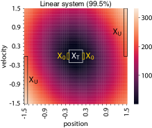
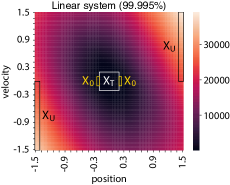
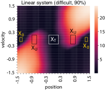
Figure 4: RASMs $V$ learned using our new method for 3 instances of linear-sys.

Robustness to input policies    We consider the same three benchmarks, but now with input policies pretrained using the Stable-Baselines3 [55] implementation of the RL algorithms TRPO, TQC, SAC, and A2C (with the default parameters; see Sect. C.1 for the loss functions for each benchmark) using a variable number of steps. The run times in Fig. 3 show that our method is generally agnostic to the algorithm used to train the policy. We observe that training policies longer does not significantly influence the time for our method to verify the policy, except when the training did not converge yet (e.g., for A2C on pendulum, cf. Sect. D.2). In particular, the input policies are trained by minimizing rewards, which does not necessarily correspond with satisfying the reach-avoid specification.

Lipschitz constants    We demonstrate the need for our efficient method to compute Lipschitz constants when solving Problem 1. We compare our techniques from Sect. 4 against the anytime algorithm LipBaB [16] on the final policy and certificate networks (cf. Sect. D.3). Our method takes $0.2\text{\,}\mathrm{s}$ to compute a Lipschitz constant (and only $0.0002\text{\,}\mathrm{s}$ when already JIT-compiled). LipBaB returns a first Lipschitz constant after $0.4\text{\,}\mathrm{s}$ (which is, on average, 20% larger than ours) and requires (for policy networks with 2 and 3 hidden layers, respectively) at least $27$ and $90\text{\,}\mathrm{s}$ to compute a better Lipschitz constant than ours. A typical benchmark requires 10–30 verifier iterations, each of which takes around $20\text{\,}\mathrm{s}$, so better results from LipBaB may not outweigh the increase in verifier run time.

Scaling up    We demonstrate that our method is able to handle benchmarks that were out of reach for the baseline (detailed results are in Sect. D.4). First, for the more difficult instance of linear-sys shown in Fig. 4, our method is able to solve Problem 1 with up to $\rho=90\%$. As shown in Fig. 4, the resulting RASM requires a less trivial (non-convex) shape than for the original instances. Second, we consider a new benchmark, triple-integrator, which has a 3D state space (see Sect. C.1 for the dynamics). We are able to solve Problem 1 with up to $\rho=95\%$. Notably, the novel local refinement scheme reduces the total discretized points needed by the verifier by multiple orders of magnitude compared to a verifier that uses a uniform discretization.

Limitations    Our main contributions focus on optimizing the procedure used by the verifier. Thus, the next points are not addressed by our experiments. (1) We did not consider the robustness w.r.t. the loss functions used for pretraining and the learner. (2) The robustness w.r.t. the initial mesh size was not considered. (3) We did not consider the scalability to benchmarks beyond 3D state spaces. (4) Our experiments are limited to three benchmarks from the literature and two novel benchmarks.

7 Conclusion

We presented two contributions to making the verification of neural network policies more scalable. First, we compute tight bounds on Lipschitz constants by integrating the novel idea of weighted norms with averaged activation operators. We further improve Lipschitz constants locally using properties of the Softplus activation function. Second, we use a local refinement scheme that uses a fine discretization where needed while keeping a coarse discretization where sufficient.

Future work includes generalizing our method for computing bounds on Lipschitz constants to broader classes of neural networks. In addition, while this work focuses on the verifier, improving the learner and the choice of counterexamples can improve the overall performance of the learner-verifier framework. Finally, we wish to investigate whether the updating of the policy within the learner can handle perturbations and uncertainty in the system dynamics and the reach-avoid specification.

Appendix A Further Algorithmic Details

A.1 Averaged Activation Operators

In this appendix, we give details regarding the integration of weighted norms and averaged activation operators [13, 27] mentioned in Sect. 4.1. Let $L_{T}$ denote the Lipschitz constant of the neural network operator $T$. We first introduce averaged activation operators, and thereafter explain how we combine this with our weighted norms.

Definition 7.

An $\alpha$-averaged activation operator ($0<\alpha<1$) is an operator $R\colon\mathbb{R}\rightarrow\mathbb{R}$ that satisfies $R=(1-\alpha)\mathrm{Id}+\alpha Q$ for some $Q\colon\mathbb{R}\rightarrow\mathbb{R}$ with Lipschitz constant $1$ and identity function $\mathrm{Id}$.

Since $\mathrm{ReLU}(x)=\tfrac{1}{2}x+\tfrac{1}{2}|x|$, the $\mathrm{ReLU}$ is $\tfrac{1}{2}$-averaged. For simplicity, we only consider $\tfrac{1}{2}$-averaged activation operators. We extend a result of Combettes and Pesquet [27] to weighted norms.

Theorem 4 (proof in Sect. B.10).

Consider an $(n+1)$-layer neural network with $\tfrac{1}{2}$-averaged activation operators $R_{k}$. Let $\mathcal{W}$ be a corresponding weight system. Let

$$S_{n}=\{(k_{1},k_{2},\ldots,k_{r})\in\mathbb{N}_{0}^{r}\mid 0\leq r\leq n-1,\,1\leq k_{1}<k_{2}<\dots<k_{r}\leq n-1\}.$$

Then the Lipschitz constant $L_{T}$ of the corresponding neural network operator $T$ satisfies

$$L_{T}\leq\frac{1}{2^{n-1}}\sum_{(k_{1},k_{2},\ldots,k_{r})\in S_{n}}\;\left[\prod_{\ell=1}^{r+1}\|A_{k_{\ell}}\ldots A_{k_{\ell-1}+1}\|^{k_{\ell-1},k_{\ell}}_{\mathcal{W}}\right],$$

where we set $k_{0}=0$ and $k_{r+1}=n$.

For $n=2$, this yields $L_{T}\leq\tfrac{1}{2}\left(\|A_{1}A_{0}\|_{\mathcal{W}}^{0,2}+\|A_{1}\|_{\mathcal{W}}^{1,2}\|A_{0}\|_{\mathcal{W}}^{0,1}\right)$. By the sub-multiplicativity of the matrix norm, it follows that this is smaller than $\|A_{1}\|_{\mathcal{W}}^{1,2}\|A_{0}\|_{\mathcal{W}}^{0,1}$.

In the general case, the sub-multiplicativity of the matrix norm implies that each of the $2^{n-1}$ summands in the sum, and hence bound, is at most $\prod_{\ell=1}^{n}\|A_{\ell}\|_{\mathcal{W}}^{\ell-1,\ell}$. Hence, the bound in Theorem 4 is (for given weights $\mathcal{W}$) tighter than the bound $\prod_{\ell=1}^{n}\|A_{\ell}\|^{\ell-1,\ell}_{\mathcal{W}}$. The intuition for the result is that for the ‘identity part’ of the averaged activation operator, we can take the matrix product inside the matrix norm (which gives a smaller result than taking the product of the matrix norms). For more intuition regarding this result in the case of unweighted norms, we refer to [27].

Note that the fact that Theorem 4 yields tighter bounds does not contradict Theorem 2, since Theorem 2 only applies if the formula $\prod_{\ell=1}^{n}\|A_{\ell}\|^{\ell-1,\ell}_{\mathcal{W}}$ is used to compute the Lipschitz bound, while the bound in Theorem 4 is always smaller for given weights.

A.2 Split Lipschitz Constant of Dynamics

In this appendix, we describe an improvement over the formula $K=L_{V}L_{f}(L_{\pi}+1)$ by analyzing the Lipschitz constant of the dynamics function $f\colon\mathcal{X}\times\mathcal{U}\times\mathcal{N}\rightarrow\mathcal{X}$ more carefully. Note that for $L_{f}$, we are interested in changes in the inputs $\mathbf{x}\in\mathcal{X}$ and $\mathbf{u}\in\mathcal{U}$, but take $\omega\in\mathcal{N}$ fixed. Hence, the Lipschitz constant $L_{f}$ satisfies

$$\|f(\mathbf{x}^{\prime},\mathbf{u}^{\prime},\omega)-f(\mathbf{x},\mathbf{u},\omega)\|\leq L_{f}\|(\mathbf{x}^{\prime},\mathbf{u}^{\prime})-(\mathbf{x},\mathbf{u})\|.$$

for all (fixed) $\omega\in\mathcal{N}$ and all $(\mathbf{x},\mathbf{u}),(\mathbf{x}^{\prime},\mathbf{u}^{\prime})\in\mathcal{X}\times\mathcal{U}$. We now compute two ‘split’ Lipschitz constants: one Lipschitz constant $L_{f,\mathbf{x}}$ corresponding to changes in the state $\mathbf{x}$ (but keeping the control fixed), and one Lipschitz constant $L_{f,\mathbf{u}}$ corresponding to changes in the control $\mathbf{u}$ (but keeping the state fixed). Formally, we have

$$\|f(\mathbf{x}^{\prime},\mathbf{u},\omega)-f(\mathbf{x},\mathbf{u},\omega)\|\leq L_{f,\mathbf{x}}\|\mathbf{x}^{\prime}-\mathbf{x}\|$$

for fixed $\mathbf{u}\in\mathcal{U}$ and $\omega\in\mathcal{N}$, and all $\mathbf{x},\mathbf{x}^{\prime}\in\mathcal{X}$. Similarly, we have

$$\|f(\mathbf{x},\mathbf{u}^{\prime},\omega)-f(\mathbf{x},\mathbf{u},\omega)\|\leq L_{f,\mathbf{u}}\|\mathbf{u}^{\prime}-\mathbf{u}\|$$

for fixed $\mathbf{x}\in\mathcal{X}$ and $\omega\in\mathcal{N}$, and all $\mathbf{u},\mathbf{u}^{\prime}\in\mathcal{U}$. For a given dynamics function $f$, we can compute (upper bounds for) $L_{f,\mathbf{x}}$ and $L_{f,\mathbf{u}}$. Note that we always have $L_{f,\mathbf{x}},L_{f,\mathbf{u}}\leq L_{f}$.

We now explain why we can replace $L_{f}(L_{\pi}+1)$ by $L_{f,\mathbf{x}}+L_{f,\mathbf{u}}L_{\pi}$, as bound for the Lipschitz constant of the function $\mathbf{x}\mapsto f(\mathbf{x},\pi(\mathbf{x}),\omega)$ for all fixed $\omega\in\mathcal{N}$.

Fix $\omega\in\mathcal{N}$, and let $\mathbf{x},\mathbf{x}^{\prime}\in\mathcal{X}$ be given. Then $\|\pi(\mathbf{x})-\pi(\mathbf{x}^{\prime})\|\leq L_{\pi}\|\mathbf{x}-\mathbf{x}^{\prime}\|$. Now we use the triangle inequality to separate the changes in $\mathbf{x}$ from those in $\mathbf{u}=\pi(\mathbf{x})$:

$$\|f(\mathbf{x},\pi(\mathbf{x}),\omega) -f(\mathbf{x}^{\prime},\pi(\mathbf{x}^{\prime}),\omega)\|$$

$$\leq\|f(\mathbf{x},\pi(\mathbf{x}),\omega)-f(\mathbf{x}^{\prime},\pi(\mathbf{x}),\omega)\|+\|f(\mathbf{x}^{\prime},\pi(\mathbf{x}),\omega)-f(\mathbf{x}^{\prime},\pi(\mathbf{x}^{\prime}),\omega)\|$$

$$\leq L_{f,\mathbf{x}}\|\mathbf{x}^{\prime}-\mathbf{x}\|+L_{f,\mathbf{u}}\|\pi(\mathbf{x})-\pi(\mathbf{x}^{\prime})\|$$

$$\leq(L_{f,\mathbf{x}}+L_{f,\mathbf{u}}L_{\pi})\|\mathbf{x}^{\prime}-\mathbf{x}\|,$$

which shows that $L_{f,\mathbf{x}}+L_{f,\mathbf{u}}L_{\pi}$ is an upper bound for the Lipschitz constant of the function $\mathbf{x}\mapsto f(\mathbf{x},\pi(\mathbf{x}),\omega)$. Hence, $L_{V}(L_{f,\mathbf{x}}+L_{f,\mathbf{u}}L_{\pi})$ is an upper bound for the Lipschitz constant of the function $\mathbf{x}\mapsto V(f(\mathbf{x},\pi(\mathbf{x}),\omega))$.

Finally, note that the inequalities $L_{f,\mathbf{x}},L_{f,\mathbf{u}}\leq L_{f}$ imply that $L_{V}(L_{f,\mathbf{x}}+L_{f,\mathbf{u}}L_{\pi})\leq L_{V}L_{f}(L_{\pi}+1)$, so replacing $K=L_{V}L_{f}(L_{\pi}+1)$ by $K=L_{V}(L_{f,\mathbf{x}}+L_{f,\mathbf{u}}L_{\pi})$ is indeed an improvement.

In practice, we have implemented this improvement in our method and all verifier variants for which we report results (including the baseline).

A.3 Suggested Mesh Size

Recall from Sect. 5 that refining the mesh size by a fixed factor $C\in(0,1)$ may be unnecessary to mitigate violations of the RASM conditions. In this section, we explain how we compute a suggested mesh for each of the points $\tilde{\mathbf{x}}\in\widetilde{\mathcal{X}}$ that violate the expected decrease condition. This suggested mesh is used as an upper bound on the factor by which we refine the discretization.

Concretely, let $\tilde{\mathbf{x}}\in\widetilde{\mathcal{X}}$ be a soft violation (as defined in Sect. 5) and denote its current mesh size by $\tau_{\tilde{\mathbf{x}}}$. Thus, $\tilde{\mathbf{x}}$ is associated with the cell $\mathrm{cell}_{\infty}^{\tau_{\tilde{\mathbf{x}}}}(\tilde{\mathbf{x}})$. For each such point, the suggested mesh $\lambda_{\tilde{\mathbf{x}}}$ is computed as

$$\lambda_{\tilde{\mathbf{x}}}=0.9\max\left\{\frac{V(\tilde{\mathbf{x}})-\mathbb{E}_{\omega\sim\mu}\left[V(f(\tilde{\mathbf{x}},\pi(\tilde{\mathbf{x}}),\omega))\right]}{K\cdot\text{SoftPlusLip}(\tilde{\mathbf{x}})+L_{V}},\frac{V_{\mathrm{LB}}(\tilde{\mathbf{x}})-\mathbb{E}_{\omega\sim\mu}\left[V(f(\tilde{\mathbf{x}},\pi(\tilde{\mathbf{x}}),\omega))\right]}{K\cdot\text{SoftPlusLip}(\tilde{\mathbf{x}})}\right\},$$ (5)

where

$$\text{SoftPlusLip}(\tilde{\mathbf{x}})=\begin{cases}1-e^{-V(\tilde{\mathbf{x}})}&\text{if }\tau Ke^{-V_{\mathrm{LB}}(\tilde{\mathbf{x}})}\geq 1\\ 1-e^{-V_{\mathrm{LB}}(\tilde{\mathbf{x}})}&\text{if }\tau Ke^{-V_{\mathrm{LB}}(\tilde{\mathbf{x}})}<1,\end{cases}$$

in accordance with Lemma 5. (In variants of the verifier where the SoftPlusLip improvement from Sect. 4.2 is not enabled, we set $\text{SoftPlusLip}(\tilde{\mathbf{x}})=1$ in the suggested mesh).

Then, our local refinement scheme splits the cell $\mathrm{cell}_{\infty}^{\tau_{\tilde{\mathbf{x}}}}(\tilde{\mathbf{x}})$ associated with the point $\tilde{\mathbf{x}}$ into smaller cells with a mesh size of $\max(C\tau_{\tilde{\mathbf{x}}},\lambda_{\tilde{\mathbf{x}}})$. As such, we refine the mesh size by the maximum of the fixed factor $C$ and the suggested mesh size $\lambda_{\tilde{\mathbf{x}}}$.

Intuition for the suggested mesh size formula

We now explain the intuition behind Eq. 5. Recall that the requirement to check the cell containing $\tilde{\mathbf{x}}$ (from Eq. 4) is that

$$\mathbb{E}_{\omega\sim\mu}\left[V(f(\tilde{\mathbf{x}},\pi(\tilde{\mathbf{x}}),\omega))\right]<V_{\mathrm{LB}}(\tilde{\mathbf{x}})-\tau_{\tilde{\mathbf{x}}}K\cdot\text{SoftPlusLip}(\tilde{\mathbf{x}}).$$

Hence, if we refine the mesh to $\lambda_{\tilde{\mathbf{x}}}<\frac{V_{\mathrm{LB}}(\tilde{\mathbf{x}})-\mathbb{E}_{\omega\sim\mu}\left[V(f(\tilde{\mathbf{x}},\pi(\tilde{\mathbf{x}}),\omega))\right]}{K\cdot\text{SoftPlusLip}(\tilde{\mathbf{x}})}$ (the second term in the maximum in Eq. 5), then the condition will be guaranteed to hold for the new cell containing $\tilde{\mathbf{x}}$. However, refining the point $\tilde{\mathbf{x}}$ introduces new points in the discretization in the cell $\mathrm{cell}_{\infty}^{\tau_{\tilde{\mathbf{x}}}}(\tilde{\mathbf{x}})$, and for these points, this suggested mesh is not necessarily sufficient. We, therefore, multiply with $0.9$ to make it more likely that the suggested mesh is also sufficient at points that are close to $\tilde{\mathbf{x}}$. This suggested mesh is somewhat conservative, however, since it does not take into account that also $V_{\mathrm{LB}}(\tilde{\mathbf{x}})$ would become larger when decreasing the mesh. The first term in the maximum in Eq. 5 takes this into account by replacing $V_{\mathrm{LB}}(\tilde{\mathbf{x}})$ by $V(\tilde{\mathbf{x}})-\tau_{\tilde{\mathbf{x}}}L_{V}$, which is also a lower bound for $V_{\mathrm{min}}(\tilde{\mathbf{x}})$ (which is almost always weaker since IBP almost always gives better bounds than using Lipschitz constants). When doing this, the requirement becomes

$$\mathbb{E}_{\omega\sim\mu}\left[V(f(\tilde{\mathbf{x}},\pi(\tilde{\mathbf{x}}),\omega))\right]<V(\tilde{\mathbf{x}})-\tau_{\tilde{\mathbf{x}}}(K\cdot\text{SoftPlusLip}(\tilde{\mathbf{x}})+L_{V}).$$

Hence, if we refine the mesh to $\lambda_{\tilde{\mathbf{x}}}<\frac{V(\tilde{\mathbf{x}})-\mathbb{E}_{\omega\sim\mu}\left[V(f(\tilde{\mathbf{x}},\pi(\tilde{\mathbf{x}}),\omega))\right]}{K\cdot\text{SoftPlusLip}(\tilde{\mathbf{x}})+L_{V}}$ (the first term in the maximum in Eq. 5), then the condition will be guaranteed to hold for the new cell containing $\tilde{\mathbf{x}}$. We again multiply by $0.9$ to take into account that the required mesh might be lower for nearby points. This is also conservative because $V_{\mathrm{LB}}(\tilde{\mathbf{x}})$ is typically larger than $V(\tilde{\mathbf{x}})-\tau_{\tilde{\mathbf{x}}}L_{V}$. By taking the maximum of these two conservative estimates, we obtain an estimate that is less conservative.

Initial and safety conditions

For the initial and safety conditions, computing a suggested mesh size is difficult due to the use of IBP for computing $V_{\mathrm{LB}}(\tilde{\mathbf{x}})$ and $V_{\mathrm{UB}}(\tilde{\mathbf{x}})$. In particular, the suggested mesh computation in Eq. 5 relies on Lipschitz constants, which are more conservative than the bounds we obtain using IBP. As a result, adapting Eq. 5 for the initial and safety conditions would lead to suggested meshes that are too conservative (i.e., too low). Thus, we simply use the fixed factor $C$ for refining violations of the initial and safety conditions.

A.4 Loss Function Learner

The learner learns a policy $\pi$ and candidate RASM $V$ by minimizing the loss function

$$\mathcal{L}(\pi,V)=\mathcal{L}_{\text{Init}}(V)+\mathcal{L}_{\text{Unsafe}}(V)+\mathcal{L}_{\text{Decr}}(\pi,V),$$

where each of the three terms model a loss resulting from violating one of the RASM conditions. The points over which we check the conditions consist of randomly sampled points and counterexamples. For each condition, we have a term based on all points sampled for that condition and a term based on counterexamples for that condition. Denote the sets of all points per condition by $P_{\text{Init}}$, $P_{\text{Unsafe}}$ and $P_{\text{Decr}}$ respectively. Denote the sets of counterexamples per condition by $C_{\text{Init}}$, $C_{\text{Unsafe}}$ and $C_{\text{Decr}}$, respectively. Let $\epsilon\in\mathbb{R}_{\geq 0}$ and let $\beta_{\mathbf{x}}\in\mathbb{R}_{\geq 0}$ be weights that we explain later on in this appendix. We now give the three terms from the loss function:

$$\mathcal{L}_{\text{Init}}(V) =\max_{\mathbf{x}\in P_{\text{Init}}}\left\{\max\{V(\mathbf{x})-1+\varepsilon,0\}\right\}$$

$$\quad+\frac{1}{\sum_{\mathbf{x}\in C_{\text{Init}}}\!\beta_{\mathbf{x}}}\sum_{\mathbf{x}\in C_{\text{Init}}}\beta_{\mathbf{x}}\max\{V(\mathbf{x})-1+\varepsilon,0\},$$

$$\mathcal{L}_{\text{Unsafe}}(V) =(1-\rho)\max_{\mathbf{x}\in P_{\text{Unsafe}}}\left\{\max\big{\{}\tfrac{1}{1-\rho}-V(\mathbf{x})+\varepsilon,0\big{\}}\right\}$$

$$\quad+\frac{1}{\sum_{\mathbf{x}\in C_{\text{Unsafe}}}\beta_{\mathbf{x}}}\sum_{\mathbf{x}\in C_{\text{Unsafe}}}\beta_{\mathbf{x}}\max\{\tfrac{1}{1-\rho}-V(\mathbf{x})+\varepsilon,0\},$$

$$\mathcal{L}_{\text{Decr}}(\pi,V) =10\sqrt{\frac{1}{|C_{\text{Decr}}|}\sum_{\mathbf{x}\in C_{\text{Decr}}}\!\!\!\max\left\{\frac{1}{N}\sum_{\omega_{i}\sim d}V(f(\mathbf{x},\pi(\mathbf{x}),\omega_{i}))-V(\mathbf{x})+\tau K^{\prime},0\right\}^{2}}$$

$$\quad+10\sqrt{\frac{1}{\sum_{\mathbf{x}\in C_{\text{Decr}}}\beta_{\mathbf{x}}}\!\!\sum_{\mathbf{x}\in C_{\text{Decr}}}\!\!\!\beta_{\mathbf{x}}\max\left\{\!\frac{1}{N}\!\!\sum_{\omega_{i}\sim d}\!V(f(\mathbf{x},\pi(\mathbf{x}),\omega_{i}))\!-\!V(\mathbf{x})\!+\!\tau K^{\prime},0\right\}^{2}}.$$

Here $K^{\prime}=K+L_{V}=L_{V}(L_{f}(L_{\pi}+1)+1)$, and $\tau$ is a loss mesh size chosen specifically for the problem. We discuss this loss mesh $\tau$ in Sect. C.2. The first term in each of the losses is taken over all points, and the second term is taken over counterexamples previously found by the verifier.

We first explain the first half term of each of the three losses (i.e., over all points). Following [73], we let the initial and unsafe loss punish the maximum violation. The $\varepsilon$ in these loss functions (which we set to $10^{-2}$) ensures that the conditions hold amply (which is required because we use IBP). The multiplier of $1-\rho$ is added on the unsafe loss to prevent the unsafe loss from taking very large values in the first training iteration, which can lead to ‘overshooting’ the minimal value $\frac{1}{1-\rho}$. For the expected decrease loss, we use a quadratic mean over all violations. Compared to an arithmetic mean, this punishes large violations relatively more than small violations. The multiplier 10 was chosen to ensure that the three conditions weigh about equally in practice.

To focus more on counterexamples (and especially on hard violations as defined in Sect. 5), we have added a weighted loss over the counterexamples found by the verifier in previous iterations. Each counterexample $\mathbf{x}$ has a weight $\beta_{\mathbf{x}}$. For counterexamples to the initial condition and the unsafe condition, the weight is 1 for soft violations and 10 for hard violations. For counterexamples to the expected decrease condition, the weight is $\max\{\mathbb{E}_{\omega\sim\mu}\left[V(f(\tilde{\mathbf{x}},\pi(\tilde{\mathbf{x}}),\omega))\right]-V(\tilde{\mathbf{x}})+\tau K,0\}$, multiplied by 10 for hard violations.

In addition, Zikelic et al. [73] also use losses penalizing the Lipschitz constant of the policy and the RASM candidate, and an auxiliary loss term that attempts to ensure that the global minimum of the candidate RASM is in the target set. We do not use these additional terms. The aim of the Lipschitz loss is to reduce the Lipschitz constant of (mainly) the certificate in fewer learner-verifier iterations. However, our method already substantially reduces the Lipschitz constant, so this additional loss has no substantial effect in combination with our method. In addition, the Lipschitz loss needs the desired Lipschitz constant as a hyperparameter, and setting it too small can actually hamper convergence. For the auxiliary loss, we observed that for high probability bounds this loss even worsens performance.

Appendix B Proofs

B.1 Preliminary Properties

We first recall several standard properties of norms and Lipschitz constants. Throughout the appendix, superscripts on norms denote the index of the norm.

Properties 1 and 2 are standard properties of Lipschitz constants.

Property 1.

If $f\colon\mathbb{R}^{m_{k}}\rightarrow\mathbb{R}^{m_{\ell}},g\colon\mathbb{R}^{m_{j}}\rightarrow\mathbb{R}^{m_{k}}$ are Lipschitz continuous with Lipschitz constants $L_{f}$ and $L_{g}$ with respect to given norms $\|\cdot\|^{j}$, $\|\cdot\|^{k}$, and $\|\cdot\|^{\ell}$ defined on $\mathbb{R}^{m_{j}}$, $\mathbb{R}^{m_{k}}$, and $\mathbb{R}^{m_{\ell}}$ respectively, then $f\circ g\colon\mathbb{R}^{m_{j}}\rightarrow\mathbb{R}^{m_{\ell}}$ is Lipschitz continuous with Lipschitz constant $L_{f}L_{g}$.

Property 2.

If $f,g\colon\mathbb{R}^{m_{k}}\rightarrow\mathbb{R}^{m_{\ell}}$ are Lipschitz continuous with Lipschitz constants $L_{f}$ and $L_{g}$ with respect to given norms $\|\cdot\|^{k}$, and $\|\cdot\|^{\ell}$ defined on $\mathbb{R}^{m_{k}}$ and $\mathbb{R}^{m_{\ell}}$ respectively, and $\alpha,\beta\in\mathbb{R}$, then $\alpha f+\beta g\colon\mathbb{R}^{m_{k}}\rightarrow\mathbb{R}^{m_{\ell}}$ is Lipschitz continuous with Lipschitz constant $|\alpha|L_{f}+|\beta|L_{g}$.

Property 3 states that the operator norm of a matrix $A$ is a Lipschitz constant of a corresponding affine function $x\mapsto Ax+b$, where $b$ is some (bias) vector.

Property 3.

Let $A\in\mathbb{R}^{m_{\ell}\times m_{k}}$ be a matrix and let $b\in\mathbb{R}^{m_{\ell}}$ be a vector. Equip the input space with the norm $\|\cdot\|^{k}$ and the output space with the norm $\|\cdot\|^{\ell}$, and let the corresponding operator norm be given by $\|A\|^{k,\ell}=\sup\Big{\{}\frac{\|Ax\|^{\ell}}{\|x\|^{k}}~{}\Big{|}~{}x\in\mathbb{R}^{m_{k}},x\neq 0\Big{\}}$. For these norms, the function $x\mapsto Ax+b$ is Lipschitz continuous with Lipschitz constant $\|A\|^{k,\ell}$.

Proof.

Let $x,x^{\prime}\in\mathbb{R}^{m_{k}}$ be given. If $x=x^{\prime}$, then $\|(Ax+b)-(Ax^{\prime}+b)\|^{\ell}=0=\|A\|^{k,\ell}\|x-x^{\prime}\|^{k}$ trivially. Now assume that $x\neq x^{\prime}$, then $x-x^{\prime}\neq 0$. Hence,

$$\|(Ax+b)-(Ax^{\prime}+b)\|^{\ell}=\|A(x-x^{\prime})\|^{\ell}\leq\|A\|^{k,\ell}\|x-x^{\prime}\|^{k},$$

which shows that $x\mapsto Ax+b$ is Lipschitz continuous with Lipschitz constant $\|A\|^{k,\ell}$. ∎

Property 4 shows that an activation function applying a scalar function componentwise inherits the Lipschitz constant of the scalar function in any weighted $1$-norm.

Property 4.

Let $R\colon\mathbb{R}\rightarrow\mathbb{R}$ be a function with Lipschitz constant $L$, i.e. $|R(x)-R(x^{\prime})|\leq L|x-x^{\prime}|$. Then the vectorized function $R^{\prime}\colon\mathbb{R}^{v}\rightarrow\mathbb{R}^{v}$ applying $R$ componentwise has Lipschitz constant $L$ when the input and output space are both equipped with the same weighted $1$-norm.

Proof.

Let $\|x\|_{\mathcal{W}}=\sum_{i=1}^{v}w_{i}\lvert x_{i}\rvert$ for weights $w_{i}>0$ be the norm on the input and output space. For any $x,x^{\prime}\in\mathbb{R}^{v}$, it holds that

$$\|R^{\prime}(x)-R^{\prime}(x^{\prime})\|_{\mathcal{W}} =\sum_{i=1}^{v}w_{i}\lvert(R^{\prime}(x)-R^{\prime}(x^{\prime}))_{i}\rvert=\sum_{i=1}^{v}w_{i}\lvert R(x_{i})-R(x^{\prime}_{i})\rvert$$

$$\leq\sum_{i=1}^{v}w_{i}L\lvert x_{i}-x^{\prime}_{i}\rvert=L\sum_{i=1}^{v}w_{i}\lvert x_{i}-x^{\prime}_{i}\rvert=L\|x-x^{\prime}\|_{\mathcal{W}},$$

which shows that $R^{\prime}$ is Lipschitz continuous with Lipschitz constant $L$. ∎

Finally, Property 5 shows how we can decompose $1$-norms.

Property 5.

Equip $\mathbb{R}^{v_{1}+v_{2}}$, $\mathbb{R}^{v_{1}}$ and $\mathbb{R}^{v_{2}}$ with a weighted $1$-norm, such that the first $v_{1}$ weights on $\mathbb{R}^{v_{1}+v_{2}}$ coincide with the weights on $\mathbb{R}^{v_{1}}$ and the last $v_{2}$ weights on $\mathbb{R}^{v_{1}+v_{2}}$ coincide with the weights on $\mathbb{R}^{v_{2}}$. Let $x=(y,z)\in\mathbb{R}^{v_{1}+v_{2}}$ with $y\in\mathbb{R}^{v_{1}}$ and $z\in\mathbb{R}^{v_{2}}$ be given. Then $\|x\|_{\mathcal{W}}\leq\|y\|_{\mathcal{W}}+\|z\|_{\mathcal{W}}$.

Proof.

The triangle inequality implies

$$\|x\|_{\mathcal{W}}=\|(y,0)+(0,z)\|_{\mathcal{W}}\leq\|(y,0)\|_{\mathcal{W}}+\|(0,z)\|_{\mathcal{W}}=\|y\|_{\mathcal{W}}+\|z\|_{\mathcal{W}},$$

where the last equality holds since from the definition of the weighted $1$-norm it follows that 0 components do not contribute to the norm. ∎

B.2 Proof of Theorem 1

We give a short proof of Theorem 1. Another proof is given in [73].

Theorem 1.

If there exists a RASM, then the reach-avoid specification is satisfied.

Proof.

Fix a policy $\pi$. We consider the stochastic process $(\mathbf{x}_{t})_{t\in\mathbb{N}_{0}}$ which is defined recursively by $\mathbf{x}_{t+1}=f(\mathbf{x}_{t},\pi(\mathbf{x}_{t}),\omega_{t})$. Let $\mathcal{F}_{t}$ be the natural filtration corresponding to $(\mathbf{x}_{t})_{t\in\mathbb{N}_{0}}$. Let

$$\sigma=\min\{t\in\mathbb{N}_{0}\colon\mathbf{x}_{t}\in\mathcal{X}_{T}\vee V(\mathbf{x}_{t})\geq\tfrac{1}{1-\rho}\}.$$

Then $\sigma$ is a stopping time, since $\{\sigma=t\}\in\mathcal{F}_{t}$ for all $t\in\mathbb{N}_{0}$; intuitively, this means that whether the event occurs is determined by the values of $\mathbf{x}_{t^{\prime}}$ for $t^{\prime}\leq t$.

The expected decrease condition implies that $(V(\mathbf{x}_{\min\{t,\sigma\}}))_{t\in\mathbb{N}_{0}}$ is a supermartingale with respect to the filtration $(\mathcal{F}_{t})_{t\in\mathbb{N}_{0}}$. Namely, if $t<\sigma$, then

$$\mathbb{E}[V(\mathbf{x}_{\min\{t+1,\sigma\}})\mid\mathcal{F}_{t}] =\mathbb{E}[V(\mathbf{x}_{t+1})\mid\mathcal{F}_{t}]=\mathbb{E}[V(f(\mathbf{x}_{t},\pi(\mathbf{x}_{t}),\omega_{t}))\mid\mathbf{x}_{t}]$$

$$=\mathbb{E}_{\omega_{t}\sim\mu}[V(f(\mathbf{x}_{t},\pi(\mathbf{x}_{t}),\omega_{t}))]\leq V(\mathbf{x}_{t})=V(\mathbf{x}_{\min\{t,\sigma\}}),$$

while if $t\geq\sigma$ then $\mathbb{E}[V(\mathbf{x}_{\min\{t+1,\sigma\}})\mid\mathcal{F}_{t}]=V(\mathbf{x}_{\sigma})=V(\mathbf{x}_{\min\{t,\sigma\}})$.

We now show that $\sigma<\infty$ almost surely (i.e., with probability 1). For this we use that $V$ decreases in expectation by $\epsilon$ each step until $\sigma$ occurs, but remains nonnegative. This implies that

$$0\leq\mathbb{E}[V(\mathbf{x}_{\min\{t,\sigma\}})]=\mathbb{E}[V(\mathbf{x}_{0})-\epsilon\sigma],$$

so $\mathbb{E}[\sigma]\leq\frac{\mathbb{E}[V(\mathbf{x}_{0})]}{\epsilon}$. Hence, Markov’s inequality implies $\mathbb{P}[\sigma\geq t]\leq\frac{\mathbb{E}[V(\mathbf{x}_{0})]}{\epsilon t}$ and taking the limit $t\rightarrow\infty$ then shows that $\sigma<\infty$ almost surely.

Since $(V(\mathbf{x}_{\min\{t,\sigma\}}))_{t\in\mathbb{N}_{0}}$ is a supermartingale and $\sigma<\infty$ almost surely, the optional stopping theorem implies that $\mathbb{E}[V(\mathbf{x}_{\sigma})]\leq\mathbb{E}[V(\mathbf{x}_{0})]$. Moreover, we have $\tfrac{1}{1-\rho}\mathbb{P}\left[V(\mathbf{x}_{\sigma})\geq\tfrac{1}{1-\rho}\right]\leq\mathbb{E}[V(\mathbf{x}_{\sigma})]$ by Markov’s inequality (using that $V$ is nonnegative), and $\mathbb{E}[V(\mathbf{x}_{0})]\leq 1$ by the initial condition. Together, this shows that $\mathbb{P}\left[V(\mathbf{x}_{\sigma})\geq\tfrac{1}{1-\rho}\right]\leq(1-\rho)\mathbb{E}[V(\mathbf{x}_{\sigma})]\leq(1-\rho)\mathbb{E}[V(\mathbf{x}_{0})]\leq 1-\rho$. Since $\mathbf{x}_{\sigma}\in\mathcal{X}_{T}\vee V(\mathbf{x}_{\sigma})\geq\frac{1}{1-\rho}$ holds, this implies $\mathbb{P}\left[\mathbf{x}_{\sigma}\in\mathcal{X}_{T}\right]\geq\rho$. Since $V(\mathbf{x}_{t})<\frac{1}{1-\rho}$ for $t<\sigma$ by the definition of $\sigma$, the safety condition guarantees that $\mathbf{x}_{t}\not\in\mathcal{X}_{U}$ for $t<\sigma$. Hence, we conclude that

$$\mathrm{Pr}^{\pi}_{\mathbf{x}_{0}}(\mathcal{X}_{T},\mathcal{X}_{U})\geq\mathbb{P}\left[\mathbf{x}_{\sigma}\in\mathcal{X}_{T}\wedge(\forall t<\sigma:\mathbf{x}_{t}\not\in\mathcal{X}_{U})\right]\geq\rho,$$

as required to show that the reach-avoid specification $(\mathcal{X}_{T},\mathcal{X}_{U},\rho)$ holds. ∎

B.3 Proof of Lemma 1

Lemma 1.

If $V$ is a discrete RASM for a discretization $\widetilde{\mathcal{X}}$, then $V$ is a RASM.

Proof.

Let $V\colon\mathcal{X}\rightarrow\mathbb{R}_{\geq 0}$ be a discrete RASM. Then $V$ is Lipschitz continuous and hence continuous. We proceed by showing that each of the three conditions in the definition of a discrete RASM (Def. 3) implies the corresponding condition in the definition of a RASM (Def. 1).

(1) Initial condition: Since $V$ is a discrete RASM, it holds that $V_{\mathrm{UB}}(\tilde{\mathbf{x}})\leq 1$ for all $\tilde{\mathbf{x}}\in\widetilde{\mathcal{X}}$ such that $\mathrm{cell}_{\infty}^{\tau}(\tilde{\mathbf{x}})\cap\mathcal{X}_{0}\neq\emptyset$. Now let $\mathbf{x}\in\mathcal{X}_{0}$ be given. Since $\widetilde{\mathcal{X}}$ is a discretization of $\mathcal{X}$, there exists a point $\tilde{\mathbf{x}}\in\widetilde{\mathcal{X}}$ such that $\mathbf{x}\in\mathrm{cell}_{\infty}^{\tau}(\tilde{\mathbf{x}})$. Then $\mathbf{x}\in\mathrm{cell}_{\infty}^{\tau}(\tilde{\mathbf{x}})\cap\mathcal{X}_{0}$, so $\mathrm{cell}_{\infty}^{\tau}(\tilde{\mathbf{x}})\cap\mathcal{X}_{0}\neq\emptyset$ and hence

$$V(\mathbf{x})\leq V_{\mathrm{max}}(\tilde{\mathbf{x}})\leq V_{\mathrm{UB}}(\tilde{\mathbf{x}})\leq 1.$$

Since $\mathbf{x}\in\mathcal{X}_{0}$ was arbitrary, we conclude that $V(\mathbf{x})\leq 1$ for all $\mathbf{x}\in\mathcal{X}_{0}$. Hence, we conclude that the Initial condition (1) from Def. 1 holds.

(2) Safety condition: Since $V$ is a discrete RASM, it holds that $V_{\mathrm{LB}}(\tilde{\mathbf{x}})\geq\frac{1}{1-\rho}$ for all $\tilde{\mathbf{x}}\in\widetilde{\mathcal{X}}$ such that $\mathrm{cell}_{\infty}^{\tau}(\tilde{\mathbf{x}})\cap\mathcal{X}_{U}\neq\emptyset$. Now let $\mathbf{x}\in\mathcal{X}_{U}$ be given. Since $\widetilde{\mathcal{X}}$ is a discretization of $\mathcal{X}$, there exists a point $\tilde{\mathbf{x}}\in\widetilde{\mathcal{X}}$ such that $\mathbf{x}\in\mathrm{cell}_{\infty}^{\tau}(\tilde{\mathbf{x}})$. Then $\mathbf{x}\in\mathrm{cell}_{\infty}^{\tau}(\tilde{\mathbf{x}})\cap\mathcal{X}_{U}$, so $\mathrm{cell}_{\infty}^{\tau}(\tilde{\mathbf{x}})\cap\mathcal{X}_{U}\neq\emptyset$ and hence

$$V(\mathbf{x})\geq V_{\mathrm{min}}(\tilde{\mathbf{x}})\geq V_{\mathrm{LB}}(\tilde{\mathbf{x}})\geq\tfrac{1}{1-\rho}.$$

Since $\mathbf{x}\in\mathcal{X}_{U}$ was arbitrary, we conclude that $V(\mathbf{x})\geq\frac{1}{1-\rho}$ for all $\mathbf{x}\in\mathcal{X}_{U}$. Hence, we conclude that the safety condition (2) from Def. 1 holds.

(3) Expected decrease condition: Since $V$ is a discrete RASM, it holds that

$$\mathbb{E}_{\omega\sim\mu}\left[V(f(\tilde{\mathbf{x}},\pi(\tilde{\mathbf{x}}),\omega))\right]<V_{\mathrm{LB}}(\tilde{\mathbf{x}})-\tau K$$

for all $\tilde{\mathbf{x}}\in\widetilde{\mathcal{X}}$ such that $\mathrm{cell}_{\infty}^{\tau}(\tilde{\mathbf{x}})\cap(\mathcal{X}\setminus\mathcal{X}_{T})\neq\emptyset$ and $V_{\mathrm{LB}}(\tilde{\mathbf{x}})<\frac{1}{1-\rho}$. For $\tilde{\mathbf{x}}\in\widetilde{\mathcal{X}}$, let

$$\epsilon_{\tilde{\mathbf{x}}}=V_{\mathrm{LB}}(\tilde{\mathbf{x}})-\tau K-\mathbb{E}_{\omega\sim\mu}\left[V(f(\tilde{\mathbf{x}},\pi(\tilde{\mathbf{x}}),\omega))\right]>0.$$

Since $\widetilde{\mathcal{X}}$ is finite, it follows that $\epsilon:=\min\limits_{\tilde{\mathbf{x}}\in\widetilde{\mathcal{X}}}\epsilon_{\tilde{\mathbf{x}}}>0$. Hence, there exists an $\epsilon>0$ such that

$$\mathbb{E}_{\omega\sim\mu}\left[V(f(\tilde{\mathbf{x}},\pi(\tilde{\mathbf{x}}),\omega))\right]\leq V_{\mathrm{LB}}(\tilde{\mathbf{x}})-\epsilon-\tau K$$

for all $\tilde{\mathbf{x}}\in\widetilde{\mathcal{X}}$ such that $\mathrm{cell}_{\infty}^{\tau}(\tilde{\mathbf{x}})\cap(\mathcal{X}\setminus\mathcal{X}_{T})\neq\emptyset$ and $V_{\mathrm{LB}}(\tilde{\mathbf{x}})<\frac{1}{1-\rho}$.

Now let $\mathbf{x}\in\mathcal{X}$ be a point such that $\mathbf{x}\in\mathcal{X}\setminus\mathcal{X}_{T}$ and $V(\mathbf{x})<\frac{1}{1-\rho}$. Since $\widetilde{\mathcal{X}}$ is a discretization of $\mathcal{X}$, there exists a point $\tilde{\mathbf{x}}\in\widetilde{\mathcal{X}}$ such that $\mathbf{x}\in\mathrm{cell}_{\infty}^{\tau}(\tilde{\mathbf{x}})$. Then $\mathbf{x}\in\mathrm{cell}_{\infty}^{\tau}(\tilde{\mathbf{x}})\cap(\mathcal{X}\setminus\mathcal{X}_{T})$, which implies $\mathrm{cell}_{\infty}^{\tau}(\tilde{\mathbf{x}})\cap(\mathcal{X}\setminus\mathcal{X}_{T})\neq\emptyset$, and $V_{\mathrm{LB}}(\tilde{\mathbf{x}})\leq V_{\mathrm{min}}(\tilde{\mathbf{x}})\leq V(\mathbf{x})<\frac{1}{1-\rho}$. Hence, we have

$$\mathbb{E}_{\omega\sim\mu}\left[V(f(\tilde{\mathbf{x}},\pi(\tilde{\mathbf{x}}),\omega))\right]\leq V_{\mathrm{LB}}(\tilde{\mathbf{x}})-\epsilon-\tau K.$$

Fix an $\omega$. Since $\mathbf{x}\in\mathrm{cell}_{\infty}^{\tau}(\tilde{\mathbf{x}})$, we have $\|\mathbf{x}-\tilde{\mathbf{x}}\|_{\infty}\leq\tau/d$, where $d$ is the dimension of the state space $\mathcal{X}$. It follows that $\|\mathbf{x}-\tilde{\mathbf{x}}\|_{1}\leq\tau$. Hence, $\|\pi(\mathbf{x})-\pi(\tilde{\mathbf{x}})\|_{1}\leq\tau L_{\pi}$, so

$$\|(\mathbf{x},\pi(\mathbf{x}),\omega)-(\tilde{\mathbf{x}},\pi(\tilde{\mathbf{x}}),\omega)\|_{1}\leq\|\mathbf{x}-\tilde{\mathbf{x}}\|_{1}+\|\pi(\mathbf{x})-\pi(\tilde{\mathbf{x}})\|_{1}\leq\tau(L_{\pi}+1),$$

by Property 5. Since $V$ and $f$ have Lipschitz constants $L_{V}$ and $L_{f}$, this implies

$$\left|V(f(\mathbf{x},\pi(\mathbf{x}),\omega))-V(f(\tilde{\mathbf{x}},\pi(\tilde{\mathbf{x}}),\omega))\right|\leq\tau L_{V}L_{f}(L_{\pi}+1)=\tau K.$$

Hence, we have $V(f(\mathbf{x},\pi(\mathbf{x}),\omega))\leq V(f(\tilde{\mathbf{x}},\pi(\tilde{\mathbf{x}}),\omega))+\tau K$ for each $\omega$. Taking the expectation over $\omega\sim\mu$ yields

$$\mathbb{E}_{\omega\sim\mu}\left[V(f(\mathbf{x},\pi(\mathbf{x}),\omega))\right] \leq\mathbb{E}_{\omega\sim\mu}\left[V(f(\tilde{\mathbf{x}},\pi(\tilde{\mathbf{x}}),\omega))\right]+\tau K$$

$$\leq V_{\mathrm{LB}}(\tilde{\mathbf{x}})-\epsilon\leq V(\mathbf{x})-\epsilon.$$

Since $\mathbf{x}\in\mathcal{X}$ was an arbitrary point such that $\mathbf{x}\in\mathcal{X}\setminus\mathcal{X}_{T}$ and $V(\mathbf{x})<\frac{1}{1-\rho}$, we conclude that there exists an $\epsilon>0$ such that $\mathbb{E}_{\omega\sim\mu}\left[V(f(\mathbf{x},\pi(\mathbf{x}),\omega))\right]\leq V(\mathbf{x})-\epsilon$ for all $\mathbf{x}\in\mathcal{X}$ such that $\mathbf{x}\in\mathcal{X}\setminus\mathcal{X}_{T}$ and $V(\mathbf{x})<\frac{1}{1-\rho}$. Hence, the Expected decrease condition (3) from Def. 1 holds.

Hence, we conclude that $V$ is a RASM, which completes the proof. ∎

B.4 Proof of Lemma 2

Lemma 2.

Let $\mathcal{W}$ be a weight system. Then $L_{T,\mathcal{W}}$ is a Lipschitz constant of $T$, i.e. $\|T(x)-T(x^{\prime})\|^{n}_{\mathcal{W}}\leq L_{T,\mathcal{W}}\|x-x^{\prime}\|^{0}_{\mathcal{W}}$ for all $x,x^{\prime}\in\mathbb{R}^{m_{0}}$. Also, if $w^{n}_{i}=1$ for all $1\leq i\leq m_{n}$, then $L_{T,\mathcal{W}}$ is also a Lipschitz constant of $T$ when equipping the input and output space with the standard (unweighted) 1-norm, i.e. $\|T(x)-T(x^{\prime})\|\leq L_{T,\mathcal{W}}\|x-x^{\prime}\|$ for all $x,x^{\prime}\in\mathbb{R}^{m_{0}}$.

Proof.

We first prove the inequality $\|T(x)-T(x^{\prime})\|^{n}_{\mathcal{W}}\leq L_{T,\mathcal{W}}\|x-x^{\prime}\|^{0}_{\mathcal{W}}$ for all $x,x^{\prime}\in\mathbb{R}^{m_{0}}$ by induction on the number of layers $(n+1)$, where $n\geq 1$.

For $n=1$, we note that

$$\|T(x)-T(x^{\prime})\|^{1}_{\mathcal{W}} =\|R_{1}(A_{1}x+b_{1})-R_{1}(A_{1}x^{\prime}+b_{1})\|^{1}_{\mathcal{W}}$$

$$\leq\|(A_{1}x+b_{1})-(A_{1}x^{\prime}+b_{1})\|^{1}_{\mathcal{W}}$$

$$\leq\|A_{1}\|^{0,1}_{\mathcal{W}}\|x-x^{\prime}\|^{0}_{\mathcal{W}}=L_{T,\mathcal{W}}\|x-x^{\prime}\|^{0}_{\mathcal{W}},$$

using Properties 3 and 4, and the fact that $R_{1}$ has Lipschitz constant 1.

For the induction step, assume that we have a network with $(n+1)+1$ layers. Write

$$T(x_{0})=R_{n+1}(A_{n+1}x_{n}+b_{n+1})=R_{n+1}(A_{n+1}T_{\leq n}(x_{0})+b_{n+1})$$

where $T_{\leq n}$ represents the operator corresponding to the first $n+1$ layers of the network. Then

$$\|T(x)-T(x^{\prime})\|^{n+1}_{\mathcal{W}} =\|R_{n+1}(A_{n+1}T_{\leq n}(x)+b_{n+1})-R_{n+1}(A_{n+1}T_{\leq n}(x^{\prime})+b_{n+1})\|^{n+1}_{\mathcal{W}}$$

$$\leq\|(A_{n+1}T_{\leq n}(x)+b_{n+1})-(A_{n+1}T_{\leq n}(x^{\prime})+b_{n+1})\|^{n+1}_{\mathcal{W}}$$

$$\leq\|A_{n+1}\|^{n,n+1}_{\mathcal{W}}\|T_{\leq n}(x)-T_{\leq n}(x^{\prime})\|^{n}_{\mathcal{W}}\leq\|A_{n+1}\|^{n,n+1}_{\mathcal{W}}L_{T_{\leq n},\mathcal{W}}\|x-x^{\prime}\|^{0}_{\mathcal{W}}$$

$$=\|A_{n+1}\|^{n,n+1}_{\mathcal{W}}\prod_{\ell=1}^{n}\|A_{\ell}\|^{\ell-1,\ell}_{\mathcal{W}}\|x-x^{\prime}\|^{0}_{\mathcal{W}}$$

$$=\prod_{\ell=1}^{n+1}\|A_{\ell}\|^{\ell-1,\ell}_{\mathcal{W}}\|x-x^{\prime}\|^{0}_{\mathcal{W}}=L_{T,\mathcal{W}}\|x-x^{\prime}\|^{0}_{\mathcal{W}},$$

which completes the induction.

We turn to the second part of the lemma. Suppose that $w_{i}^{n}=1$ for $1\leq i\leq m_{n}$. By definition of the weight system $\mathcal{W}$, we have $\max_{i}w_{i}^{0}=1$, so $w_{i}^{0}\leq 1$ for $1\leq i\leq m_{0}$. Hence, if $\|\cdot\|$ denotes the unweighted 1-norm, then $\|x\|=\|x\|_{\mathcal{W}}^{n}$ for $x\in\mathbb{R}^{m_{n}}$ and

$$\|x\|=\sum_{i=1}^{m_{0}}|x_{i}|\geq\sum_{i=1}^{m_{0}}w_{i}^{0}|x_{i}|=\|x\|_{\mathcal{W}}^{0}$$

for $x\in\mathbb{R}^{m_{0}}$. Hence, we conclude that

$$\|T(x)-T(x^{\prime})\|=\|T(x)-T(x^{\prime})\|^{n+1}_{\mathcal{W}}\leq L_{T,\mathcal{W}}\|x-x^{\prime}\|^{0}_{\mathcal{W}}\leq L_{T,\mathcal{W}}\|x-x^{\prime}\|,$$

which completes the proof. ∎

B.5 Proof of Lemma 3

Lemma 3.

If $(w^{0},K)$ is optimal for $S$, then $K\leq\widetilde{K}$ for all $(\widetilde{w}^{0},\widetilde{K})\in S$.

Proof.

Let $S$ be a set of pairs $(\widetilde{w}^{0},\widetilde{K})$ and let $(w^{0},K)$ be optimal for $S$. Then $\widetilde{K}\widetilde{w}^{0}_{j}\geq Kw^{0}_{j}$ for all $1\leq j\leq m_{0}$. By definition of a weight system, we have $\max_{j}\widetilde{w}^{0}_{j}=\max_{j}w^{0}_{j}=1$. Take a $j^{*}$ such that $w^{0}_{j^{*}}=1$. Then $\widetilde{w}^{0}_{j^{*}}\leq 1$, so $\widetilde{K}\geq\widetilde{K}\widetilde{w}^{0}_{j^{*}}\geq Kw^{0}_{j^{*}}=K$, as required. ∎

B.6 Proof of Lemma 4

Lemma 4.

Let $M\in\mathbb{R}^{m_{\ell}\times m_{k}}$ be a matrix with entries $M_{ij}$. Equip the input space with the norm $\|x\|_{\mathcal{W}}^{k}=\sum_{i=1}^{m_{k}}w_{i}^{k}\lvert x_{i}\rvert$ and the output space with the norm $\|x\|_{\mathcal{W}}^{\ell}=\sum_{i=1}^{m_{\ell}}w_{i}^{\ell}\lvert x_{i}\rvert$. Then the corresponding matrix norm satisfies $\|M\|^{k,\ell}_{\mathcal{W}}\;=\;\max\limits_{1\leq j\leq m_{k}}\left[\frac{1}{w_{j}^{k}}\sum_{i=1}^{m_{\ell}}w_{i}^{\ell}\left\lvert M_{ij}\right\rvert\right]$.

Proof.

Note that we can write $\|x\|_{\mathcal{W}}^{k}=\sum_{i=1}^{m_{k}}w_{i}^{k}\lvert x_{i}\rvert$ and $\|y\|_{\mathcal{W}}^{\ell}=\sum_{i=1}^{m_{\ell}}w_{i}^{\ell}\lvert y_{i}\rvert$. Hence,

$$\|Ax\|_{\mathcal{W}}^{\ell} =\sum_{i=1}^{m_{\ell}}w_{i}^{\ell}\lvert(Ax)_{i}\rvert\leq\sum_{i=1}^{m_{\ell}}\left[w_{i}^{\ell}\sum\limits_{j=1}^{m_{k}}\lvert A_{ij}\rvert\lvert x_{j}\rvert\right]$$

$$=\sum\limits_{j=1}^{m_{k}}\left(\frac{1}{w_{j}^{k}}\sum_{i=1}^{m_{\ell}}w_{i}^{\ell}\left\lvert A_{ij}\right\rvert\right)w_{j}^{k}\lvert x_{j}\rvert$$

$$\leq\left(\max_{1\leq j\leq m_{k}}\left[\frac{1}{w_{j}^{k}}\sum_{i=1}^{m_{\ell}}w_{i}^{\ell}\left\lvert A_{ij}\right\rvert\right]\right)\!\sum\limits_{j=1}^{m_{k}}w_{j}^{k}\lvert x_{j}\rvert$$

$$=\left(\max_{1\leq j\leq m_{k}}\left[\frac{1}{w_{j}^{k}}\sum_{i=1}^{m_{\ell}}w_{i}^{\ell}\left\lvert A_{ij}\right\rvert\right]\right)\|x\|_{\mathcal{W}}^{k},$$

which shows that $\|A\|_{\mathcal{W}}^{k,\ell}=\sup\Big{\{}\frac{\|Ax\|_{\mathcal{W}}^{\ell}}{\|x\|_{\mathcal{W}}^{k}}~{}\Big{|}~{}x\in\mathbb{R}^{m_{k}},x\neq 0\Big{\}}\leq\max\limits_{1\leq j\leq m_{k}}\left[\frac{1}{w_{j}^{k}}\sum_{i=1}^{m_{\ell}}w_{i}^{\ell}\left\lvert A_{ij}\right\rvert\right]$.

Moreover, the inequality $\|Ax\|_{\mathcal{W}}^{\ell}\leq\max\limits_{1\leq j\leq m_{k}}\left[\frac{1}{w_{j}^{k}}\sum_{i=1}^{m_{\ell}}w_{i}^{\ell}\left\lvert A_{ij}\right\rvert\right]\|x\|_{\mathcal{W}}^{k}$ holds with equality, if we choose a $j^{*}\in\operatorname*{arg\,max}\limits_{1\leq j\leq m_{k}}\left[\frac{1}{w_{j}^{k}}\sum_{i=1}^{m_{\ell}}w_{i}^{\ell}\left\lvert A_{ij}\right\rvert\right]$ and define $x$ by $x_{j^{*}}=1$ and $x_{j}=0$ for $j\neq j^{*}$. This shows that the operator norm $\|A\|_{\mathcal{W}}^{k,\ell}$ is in fact equal to $\max\limits_{1\leq j\leq m_{k}}\left[\frac{1}{w_{j}^{k}}\sum_{i=1}^{m_{\ell}}w_{i}^{\ell}\left\lvert A_{ij}\right\rvert\right]$. ∎

B.7 Proof of Theorem 2

Theorem 2.

Let output weights $w^{n}$ be given. The input weights $w^{0}$ and Lipschitz bound $K$ computed using Algorithm 1 are optimal among the set of pairs $(w^{0},L_{T,\mathcal{W}})$ that can be computed by choosing a weight system $\mathcal{W}$.

Proof.

We prove the statement by induction on the number of layers $(n+1)$, where $n\geq 1$.

For $n=1$, the pair $(w^{0},K)$ computed using Algorithm 1 satisfies $Kw_{j}^{0}=\sum_{i=1}^{m_{0}}w_{i}^{1}\left\lvert(A_{1})_{ij}\right\rvert$, while for any pair $(\widetilde{w}^{0},\widetilde{K})$ corresponding to weight system $\widetilde{\mathcal{W}}$ we have

$$\widetilde{K}\widetilde{w}_{j}^{0}=\|A_{1}\|^{0,1}_{\widetilde{\mathcal{W}}}\widetilde{w}_{j}^{0}\geq\left(\frac{1}{\widetilde{w}_{j}^{0}}\sum_{i=1}^{m_{0}}w_{i}^{1}\left\lvert(A_{1})_{ij}\right\rvert\right)\widetilde{w}_{j}^{0}=\sum\limits_{i=1}^{m_{0}}w_{i}^{1}\left\lvert(A_{1})_{ij}\right\rvert=Kw_{j}^{0}$$

by Lemma 4, showing the optimality of the pair $(w,K)$.

For the induction step, assume that we have a network with $(n+1)+1$ layers. Let $(w,K)$ denote the pair computed using Algorithm 1. Let $(w^{1},K_{\geq 2})$ denote the pair computed after all but one iteration of the outer loop, i.e. $K_{\geq 2}=\prod_{\ell=2}^{n+1}\|A_{\ell}\|^{\ell-1,\ell}_{\mathcal{W}}$. Let $K_{1}$ be the Lipschitz factor in the last iteration of the loop. Then $K=K_{1}K_{\geq 2}$. Similarly, let $(\widetilde{w},\widetilde{K})$ be any other pair computed by choosing weight system $\widetilde{\mathcal{W}}$ and using the formula $\prod_{\ell=1}^{n+1}\|A_{\ell}\|^{\ell-1,\ell}_{\widetilde{\mathcal{W}}}$. Let $(\widetilde{w}^{1},\widetilde{K}_{\geq 2})$ denote the pair corresponding to the network whose input layer is the second layer of the given network, i.e. $\widetilde{w}^{1}$ are the weights on the second layer and $\widetilde{K}_{\geq 2}=\prod_{\ell=2}^{n+1}\|A_{\ell}\|^{\ell-1,\ell}_{\widetilde{\mathcal{W}}}$. Finally, let $\widetilde{K}_{1}=\|A_{1}\|^{0,1}_{\widetilde{\mathcal{W}}}$ be the Lipschitz factor in the last iteration of the loop. Then $\widetilde{K}=\widetilde{K}_{1}^{\prime}\widetilde{K}_{\geq 2}$.

From Algorithm 1, we note that $K_{1}w_{j}^{0}=\sum_{i=1}^{m_{0}}w_{i}^{1}\left\lvert(A_{1})_{ij}\right\rvert$, while Lemma 4 implies that

$$\widetilde{K}_{1}\widetilde{w}_{j}^{0}=\|A_{1}\|^{0,1}_{\widetilde{\mathcal{W}}}\widetilde{w}_{j}^{0}\geq\left(\frac{1}{\widetilde{w}_{j}^{0}}\sum_{i=1}^{m_{0}}w^{1}_{i}\left\lvert(A_{1})_{ij}\right\rvert\right)\widetilde{w}_{j}^{0}=\sum_{i=1}^{m_{0}}\widetilde{w}^{1}_{i}\left\lvert(A_{1})_{ij}\right\rvert.$$

By the induction hypothesis, we have $\widetilde{K}_{\geq 2}\widetilde{w}^{1}_{j}\geq K_{\geq 2}w^{1}_{j}$ for all $1\leq j\leq m_{1}$. Combining yields

$$\widetilde{K}\widetilde{w}_{j}^{0}=\widetilde{K}_{1}\widetilde{K}_{\geq 2}\widetilde{w}_{j}^{0}\geq\sum_{i=1}^{m_{0}}\widetilde{K}_{\geq 2}\widetilde{w}^{1}_{i}\left\lvert(A_{1})_{ij}\right\rvert\geq\sum_{i=1}^{m_{0}}K_{\geq 2}w^{1}_{i}\left\lvert(A_{1})_{ij}\right\rvert=K_{1}K_{\geq 2}w_{j}^{0}=Kw_{j}^{0},$$

which is the required inequality. This completes the induction and hence the proof. ∎

B.8 Proof of Theorem 3

Theorem 3.

Let $V(\mathbf{x})=\mathrm{SoftPlus}(\widetilde{V}(\mathbf{x}))$ and let $L_{\widetilde{V}}$ be a Lipschitz constant for $\widetilde{V}$. Define $K=L_{\widetilde{V}}L_{f}(L_{\pi}+1)$. The inequality

$$\mathbb{E}_{\omega\sim\mu}\left[V(f(\tilde{\mathbf{x}},\pi(\tilde{\mathbf{x}}),\omega))\right]<V_{\mathrm{min}}(\tilde{\mathbf{x}})-\tau K\left(1-e^{-V_{\mathrm{min}}(\tilde{\mathbf{x}})}\right),$$

implies the expected decrease condition in Def. 1, i.e., there exists an $\epsilon>0$ such that

$$\mathbb{E}_{\omega\sim\mu}\left[V(f(\mathbf{x},\pi(\mathbf{x}),\omega))\right]\leq V(\mathbf{x})-\epsilon\quad\text{for all $\mathbf{x}\in\mathrm{cell}_{\infty}^{\tau}(\tilde{\mathbf{x}})$}.$$

Proof.

Fix an $\omega$ and let $\mathbf{x}\in\mathrm{cell}_{\infty}^{\tau}(\tilde{\mathbf{x}})$. Then we have $\|\mathbf{x}-\tilde{\mathbf{x}}\|_{\infty}\leq\tau/d$, where $d$ is the dimension of the state space $\mathcal{X}$. It follows that $\|\mathbf{x}-\tilde{\mathbf{x}}\|_{1}\leq\tau$. Hence, $\|\pi(\mathbf{x})-\pi(\tilde{\mathbf{x}})\|_{1}\leq\tau L_{\pi}$, so

$$\|(\mathbf{x},\pi(\mathbf{x}),\omega)-(\tilde{\mathbf{x}},\pi(\tilde{\mathbf{x}}),\omega)\|_{1}\leq\|\mathbf{x}-\tilde{\mathbf{x}}\|_{1}+\|\pi(\mathbf{x})-\pi(\tilde{\mathbf{x}})\|_{1}\leq\tau(L_{\pi}+1),$$

by Property 5. Since $\widetilde{V}$ and $f$ have Lipschitz constants $L_{\widetilde{V}}$ and $L_{f}$, this implies

$$\left|\widetilde{V}(f(\mathbf{x},\pi(\mathbf{x}),\omega))-\widetilde{V}(f(\tilde{\mathbf{x}},\pi(\tilde{\mathbf{x}}),\omega))\right|\leq\tau L_{V}L_{f}(L_{\pi}+1)=\tau K.$$

Hence, we have $\widetilde{V}(f(\mathbf{x},\pi(\mathbf{x}),\omega))\leq\widetilde{V}(f(\tilde{\mathbf{x}},\pi(\tilde{\mathbf{x}}),\omega))+\tau K$ for each $\omega$. Now let $t\in[0,\tau K]$ and let $v\in\mathbb{R}$. Then

$$\mathrm{SoftPlus}\left(v+t\right) =\mathrm{SoftPlus}\left(v\right)+\int_{v}^{v+t}\mathrm{SoftPlus}^{\prime}(x)\,\mathrm{d}x$$

$$=\mathrm{SoftPlus}\left(v\right)+\int_{v}^{v+t}1-e^{-\mathrm{SoftPlus}(x)}\,\mathrm{d}x$$

$$\leq\mathrm{SoftPlus}\left(v\right)+\int_{v}^{v+t}1-e^{-\mathrm{SoftPlus}(v+t)}\,\mathrm{d}x$$

$$\leq\mathrm{SoftPlus}\left(v\right)+t\left(1-e^{-\mathrm{SoftPlus}(v+t)}\right).$$

Note that $x\mapsto 1-e^{-x}$ is a concave function (the second derivative $-e^{-x}$ is negative), so Jensen’s inequality implies that $\mathbb{E}\left[1-e^{-X}\right]\leq 1-e^{-\mathbb{E}[X]}$ for any random variable $X$. If we plug in $v=\widetilde{V}(f(\tilde{\mathbf{x}},\pi(\tilde{\mathbf{x}}),\omega))$ and take the expectation, then using Jensen’s inequality, we get

$$\mathbb{E}_{\omega\sim\mu} \left[\mathrm{SoftPlus}\left(\widetilde{V}(f(\tilde{\mathbf{x}},\pi(\tilde{\mathbf{x}}),\omega))+t\right)\right]$$

$$\leq\mathbb{E}_{\omega\sim\mu}\left[\mathrm{SoftPlus}\left(\widetilde{V}(f(\tilde{\mathbf{x}},\pi(\tilde{\mathbf{x}}),\omega))\right)+t\left(1-e^{-\mathrm{SoftPlus}\left(\widetilde{V}(f(\tilde{\mathbf{x}},\pi(\tilde{\mathbf{x}}),\omega))+t\right)}\right)\right]$$

$$=\mathbb{E}_{\omega\sim\mu}\left[\mathrm{SoftPlus}\left(\widetilde{V}(f(\tilde{\mathbf{x}},\pi(\tilde{\mathbf{x}}),\omega))\right)\right]+t\;\mathbb{E}_{\omega\sim\mu}\left[1-e^{-\mathrm{SoftPlus}\left(\widetilde{V}(f(\tilde{\mathbf{x}},\pi(\tilde{\mathbf{x}}),\omega))+t\right)}\right]$$

$$\leq\mathbb{E}_{\omega\sim\mu}\left[\mathrm{SoftPlus}\left(\widetilde{V}(f(\tilde{\mathbf{x}},\pi(\tilde{\mathbf{x}}),\omega))\right)\right]+t\left(1-e^{-\mathbb{E}_{\omega\sim\mu}\left[\mathrm{SoftPlus}\left(\widetilde{V}(f(\tilde{\mathbf{x}},\pi(\tilde{\mathbf{x}}),\omega))+t\right)\right]}\right).$$

Suppose that $\mathbb{E}_{\omega\sim\mu}\left[\mathrm{SoftPlus}\left(\widetilde{V}(f(\tilde{\mathbf{x}},\pi(\tilde{\mathbf{x}}),\omega))+\tau K\right)\right]\geq V_{\mathrm{min}}(\tilde{\mathbf{x}})$. We work towards a contradiction. Note that $t\mapsto\mathbb{E}_{\omega\sim\mu}\left[\mathrm{SoftPlus}\left(\widetilde{V}(f(\tilde{\mathbf{x}},\pi(\tilde{\mathbf{x}}),\omega))+t\right)\right]$ is an increasing continuous function, since $\mathrm{SoftPlus}$ is increasing and continuous. Also, for $t=0$ we have

$$\mathbb{E}_{\omega\sim\mu}\left[\mathrm{SoftPlus}\left(\widetilde{V}(f(\tilde{\mathbf{x}},\pi(\tilde{\mathbf{x}}),\omega))+t\right)\right]=\mathbb{E}_{\omega\sim\mu}\left[V(f(\tilde{\mathbf{x}},\pi(\tilde{\mathbf{x}}),\omega))\right]<V_{\mathrm{min}}(\tilde{\mathbf{x}}).$$

Hence, by the Intermediate Value Theorem there exists a $t\in[0,\tau K]$ such that $\mathbb{E}_{\omega\sim\mu}\left[\mathrm{SoftPlus}\left(\widetilde{V}(f(\tilde{\mathbf{x}},\pi(\tilde{\mathbf{x}}),\omega))+t\right)\right]=V_{\mathrm{min}}(\tilde{\mathbf{x}})$. For this $t\leq\tau K$ we then find

$$\mathbb{E}_{\omega\sim\mu} \left[\mathrm{SoftPlus}\left(\widetilde{V}(f(\tilde{\mathbf{x}},\pi(\tilde{\mathbf{x}}),\omega))+t\right)\right]$$

$$\leq\mathbb{E}_{\omega\sim\mu}\left[\mathrm{SoftPlus}\left(\widetilde{V}(f(\tilde{\mathbf{x}},\pi(\tilde{\mathbf{x}}),\omega))\right)\right]+t\left(1-e^{-\mathbb{E}_{\omega\sim\mu}\left[\mathrm{SoftPlus}\left(\widetilde{V}(f(\tilde{\mathbf{x}},\pi(\tilde{\mathbf{x}}),\omega))+t\right)\right]}\right)$$

$$<V_{\mathrm{min}}(\tilde{\mathbf{x}})-\tau K\left(1-e^{-V_{\mathrm{min}}(\tilde{\mathbf{x}})}\right)+\tau K\left(1-e^{-V_{\mathrm{min}}(\tilde{\mathbf{x}})}\right)=V_{\mathrm{min}}(\tilde{\mathbf{x}}),$$

a contradiction. Hence, we conclude that $\mathbb{E}_{\omega\sim\mu}\left[\mathrm{SoftPlus}\left(\widetilde{V}(f(\tilde{\mathbf{x}},\pi(\tilde{\mathbf{x}}),\omega))+\tau K\right)\right]<V_{\mathrm{min}}(\tilde{\mathbf{x}})$.

This in turn implies

$$\mathbb{E}_{\omega\sim\mu} \left[V(f(\mathbf{x},\pi(\mathbf{x}),\omega))\right]$$

$$\leq\mathbb{E}_{\omega\sim\mu}\left[\mathrm{SoftPlus}\left(\widetilde{V}(f(\tilde{\mathbf{x}},\pi(\tilde{\mathbf{x}}),\omega))\right)\right]$$

$$\leq\mathbb{E}_{\omega\sim\mu}\left[\mathrm{SoftPlus}\left(\widetilde{V}(f(\tilde{\mathbf{x}},\pi(\tilde{\mathbf{x}}),\omega))+\tau K\right)\right]$$

$$\leq\mathbb{E}_{\omega\sim\mu}\left[\mathrm{SoftPlus}\left(\widetilde{V}(f(\tilde{\mathbf{x}},\pi(\tilde{\mathbf{x}}),\omega))\right)\right]+\tau K\left(1-e^{-\mathbb{E}_{\omega\sim\mu}\left[\mathrm{SoftPlus}\left(\widetilde{V}(f(\tilde{\mathbf{x}},\pi(\tilde{\mathbf{x}}),\omega))+\tau K\right)\right]}\right)$$

$$<\mathbb{E}_{\omega\sim\mu}\left[V(f(\tilde{\mathbf{x}},\pi(\tilde{\mathbf{x}}),\omega))\right]+\tau K\left(1-e^{-V_{\mathrm{min}}(\tilde{\mathbf{x}})}\right)$$

$$<V_{\mathrm{min}}(\tilde{\mathbf{x}})-\tau K\left(1-e^{-V_{\mathrm{min}}(\tilde{\mathbf{x}})}\right)+\tau K\left(1-e^{-V_{\mathrm{min}}(\tilde{\mathbf{x}})}\right)$$

$$=V_{\mathrm{min}}(\tilde{\mathbf{x}})\leq V(\mathbf{x}).$$

Hence, $V(\mathbf{x})-\mathbb{E}_{\omega\sim\mu}\left[V(f(\mathbf{x},\pi(\mathbf{x}),\omega))\right]>0$ for all $\mathbf{x}\in\mathrm{cell}_{\infty}^{\tau}(\tilde{\mathbf{x}})$. Since the function $\mathbf{x}\mapsto V(\mathbf{x})-\mathbb{E}_{\omega\sim\mu}\left[V(f(\mathbf{x},\pi(\mathbf{x}),\omega))\right]$ is continuous and the set $\mathrm{cell}_{\infty}^{\tau}(\tilde{\mathbf{x}})$ is compact, it follows by Weierstrass’ Extreme Value Theorem that $V(\mathbf{x})-\mathbb{E}_{\omega\sim\mu}\left[V(f(\mathbf{x},\pi(\mathbf{x}),\omega))\right]$ attains some positive minimum $\epsilon>0$. This implies that

$$\mathbb{E}_{\omega\sim\mu}\left[V(f(\mathbf{x},\pi(\mathbf{x}),\omega))\right]\leq V(\mathbf{x})-\epsilon\quad\text{for all $\mathbf{x}\in\mathrm{cell}_{\infty}^{\tau}(\tilde{\mathbf{x}})$},$$

completing the proof. ∎

B.9 Proof of Lemma 5

Lemma 5.

The RHS of Eq. 4 can be replaced by $V_{\mathrm{LB}}(\tilde{\mathbf{x}})-\tau K\left(1-e^{-V(\tilde{\mathbf{x}})}\right)$. If $\tau Ke^{-V_{\mathrm{LB}}(\tilde{\mathbf{x}})}<1$, then we can also replace it by $V_{\mathrm{LB}}(\tilde{\mathbf{x}})-\tau K\left(1-e^{-V_{\mathrm{LB}}(\tilde{\mathbf{x}})}\right)$.

Proof.

Note that the function $(v_{1},v_{2})\mapsto v_{1}-\tau K\left(1-e^{-v_{2}}\right)$ is increasing in $v_{1}$ but decreasing in $v_{2}$. Since $V_{\mathrm{LB}}(\mathbf{x})\leq V_{\mathrm{min}}(\mathbf{x})\leq V(\mathbf{x})$ it follows that

$$V_{\mathrm{min}}(\mathbf{x})-\tau K\left(1-e^{-V_{\mathrm{min}}(\mathbf{x})}\right)\geq V_{\mathrm{LB}}(\mathbf{x})-\tau K\left(1-e^{-V(\mathbf{x})}\right).$$

Hence, replacing the right hand side in Eq. 4 by $V_{\mathrm{LB}}(\mathbf{x})-\tau K\left(1-e^{-V(\mathbf{x})}\right)$ gives a stricter condition, as required. This proves the first part of the lemma.

Suppose that $\tau Ke^{-V_{\mathrm{LB}}(\mathbf{x})}<1$. Then the function $v\mapsto v-\tau K\left(1-e^{-v}\right)$ is increasing for $v\geq V_{\mathrm{LB}}(\mathbf{x})$, since its derivative is $v\mapsto 1-\tau Ke^{-v}$, which is positive for $v\geq V_{\mathrm{LB}}(\mathbf{x})$. Hence,

$$V_{\mathrm{min}}(\mathbf{x})-\tau K\left(1-e^{-V_{\mathrm{min}}(\mathbf{x})}\right)\geq V_{\mathrm{LB}}(\mathbf{x})-\tau K\left(1-e^{-V_{\mathrm{LB}}(\mathbf{x})}\right).$$

if $\tau Ke^{-V_{\mathrm{LB}}(\mathbf{x})}<1$. This shows that replacing the right hand side in Eq. 4 by $V_{\mathrm{LB}}(\mathbf{x})-\tau K\left(1-e^{-V_{\mathrm{LB}}(\mathbf{x})}\right)$ gives a stricter condition, which proves the second part of the lemma. ∎

B.10 Proof of Theorem 4

Theorem 4.

Consider an $(n+1)$-layer neural network with $\tfrac{1}{2}$-averaged activation operators $R_{k}$. Let $\mathcal{W}$ be a corresponding weight system. Let

$$S_{n}=\{(k_{1},k_{2},\ldots,k_{r})\in\mathbb{N}_{0}^{r}\mid 0\leq r\leq n-1,\,1\leq k_{1}<k_{2}<\dots<k_{r}\leq n-1\}.$$

Then the Lipschitz constant $L_{T}$ of the corresponding neural network operator $T$ satisfies

$$L_{T}\leq\frac{1}{2^{n-1}}\sum_{(k_{1},k_{2},\ldots,k_{r})\in S_{n}}\;\left[\prod_{\ell=1}^{r+1}\|A_{k_{\ell}}\ldots A_{k_{\ell-1}+1}\|^{k_{\ell-1},k_{\ell}}_{\mathcal{W}}\right],$$

where we set $k_{0}=0$ and $k_{r+1}=n$.

Proof.

We prove the statement by induction on the number of layers $(n+1)$, where $n\geq 1$. For the proof, we first omit the outermost activation operator. Note that the Lipschitz constant of each activation operator $R_{k}$ is 1 since it is a $\tfrac{1}{2}$-averaged activation operator and using Property 4. In particular, Property 1 shows that a Lipschitz constant computed for the network without the outermost activation operator is also valid for the network where we do have the outermost activation operator.

For $n=1$, we have $T(x_{0})=A_{1}x_{0}+b_{1}$. Then $L_{T}\leq\|A_{1}\|_{\mathcal{W}}^{0,n}$ by Property 3.

For the induction step, assume that we have a network with $(n+1)+1$ layers. Write

$$T(x_{0})=A_{n+1}x_{n}+b_{n+1}=A_{n+1}R_{n}(T_{\leq n}(x_{0}))+b_{n+1}$$

where $T_{\leq n}$ represents the operator corresponding to the first $n+1$ layers of the network. Since $R_{n}$ is $\tfrac{1}{2}$-averaged, we can write $R_{n}(x)=\tfrac{1}{2}x+\tfrac{1}{2}Q(x)$, where $Q$ has Lipschitz constant 1. Hence,

$$T(x_{0}) =\tfrac{1}{2}\left(A_{n+1}(A_{n}x_{n-1}+b_{n})+b_{n+1}\right)+\tfrac{1}{2}\left(A_{n+1}Q(T_{\leq n}(x_{0}))+b_{n+1}\right)$$

$$=\tfrac{1}{2}\left((A_{n+1}A_{n})x_{n-1}+(A_{n+1}b_{n}+b_{n+1})\right)+\tfrac{1}{2}\left(A_{n+1}Q(T_{\leq n}(x_{0}))+b_{n+1}\right)$$

$$=\tfrac{1}{2}T_{\leq n}^{\prime}(x_{0})+\tfrac{1}{2}\left(A_{n+1}Q(T_{\leq n}(x_{0}))+b_{n+1}\right),$$

where $T_{\leq n}^{\prime}$ represents the operator corresponding to a network with $n+1$ layers, where the first $n$ layers are as in the given network, but where the last layer is as the output layer of the given network, the matrix is $A_{n+1}A_{n}$ and the bias is $A_{n+1}b_{n}+b_{n+1}$. Define $A^{\prime}_{k}=A_{k}$ for $k<n$ and $A^{\prime}_{n}=A_{n+1}A_{n}$. The induction hypothesis informs us that

$$L_{T_{\leq n}^{\prime}}\leq\frac{1}{2^{n-1}}\sum_{(k_{1},k_{2},\ldots,k_{r})\in S_{n}}\;\left[\prod_{\ell=1}^{r+1}\|A^{\prime}_{k_{\ell}}\ldots A^{\prime}_{k_{\ell-1}+1}\|_{\mathcal{W}}^{k_{\ell-1},k_{\ell}}\right],$$

where in this case $k_{r+1}=n$. If we instead write $k_{r+1}=n+1$, we can also write

$$L_{T_{\leq n}^{\prime}}\leq\frac{1}{2^{n-1}}\sum_{(k_{1},k_{2},\ldots,k_{r})\in S_{n}}\;\left[\prod_{\ell=1}^{r+1}\|A_{k_{\ell}}\ldots A_{k_{\ell-1}+1}\|_{\mathcal{W}}^{k_{\ell-1},k_{\ell}}\right].$$

The induction hypothesis also informs us that

$$L_{T_{\leq n}}\leq\frac{1}{2^{n-1}}\sum_{(k_{1},k_{2},\ldots,k_{r})\in S_{n}}\;\left[\prod_{\ell=1}^{r+1}\|A_{k_{\ell}}\ldots A_{k_{\ell-1}+1}\|_{\mathcal{W}}^{k_{\ell-1},k_{\ell}}\right].$$

where $k_{r+1}=n$. Write $T^{\prime}(x)=A_{n+1}Q(T_{\leq n}(x))+b_{n+1}$. Since $Q$ has Lipschitz constant 1 and $x\mapsto A_{n+1}x+b_{n+1}$ has Lipschitz constant $\|A_{n+1}\|_{\mathcal{W}}^{n,n+1}$ by Property 3, we can bound the Lipschitz constant of $T^{\prime}$ as $L_{T^{\prime}}\leq\|A_{n+1}\|_{\mathcal{W}}^{n,n+1}L_{T_{\leq n}}$ by Property 1. We can also write this as

$$L_{T^{\prime}}\leq\frac{1}{2^{n-1}}\sum_{(k_{1},k_{2},\ldots,k_{r})\in S_{n+1}:k_{r}=n}\;\left[\prod_{\ell=1}^{r+1}\|A_{k_{\ell}}\ldots A_{k_{\ell-1}+1}\|_{\mathcal{W}}^{k_{\ell-1},k_{\ell}}\right].$$

where $k_{r+1}=n+1$.

Note that

$$S_{n+1} =\{(k_{1},k_{2},\ldots,k_{r})\mid 0\leq r\leq n,\,1\leq k_{1}<k_{2}<\dots<k_{r}\leq n\}$$

$$=S_{n}\cup\{(k_{1},k_{2},\ldots,k_{r})\mid 0\leq r\leq n,\,1\leq k_{1}<k_{2}<\dots<k_{r}\leq n,k_{r}=n\}$$

$$=S_{n}\cup\{(k_{1},k_{2},\ldots,k_{r})\in S_{n+1}\mid k_{r}=n\}.$$

Using Property 2, we find that

$$L_{T} \leq\tfrac{1}{2}L_{T^{\prime}_{\leq n}}+\tfrac{1}{2}L_{T^{\prime}}$$

$$\leq\frac{1}{2^{(n+1)-1}}\Bigg{(}\sum_{(k_{1},k_{2},\ldots,k_{r})\in S_{n}}\;\left[\prod_{\ell=1}^{r+1}\|A_{k_{\ell}}\ldots A_{k_{\ell-1}+1}\|_{\mathcal{W}}^{k_{\ell-1},k_{\ell}}\right]$$

$$\qquad\qquad\qquad\qquad+\sum_{(k_{1},k_{2},\ldots,k_{r})\in S_{n+1}:k_{r}=n}\;\left[\prod_{\ell=1}^{r+1}\|A_{k_{\ell}}\ldots A_{k_{\ell-1}+1}\|_{\mathcal{W}}^{k_{\ell-1},k_{\ell}}\right]\Bigg{)}$$

$$=\frac{1}{2^{(n+1)-1}}\sum_{(k_{1},k_{2},\ldots,k_{r})\in S_{n+1}}\;\left[\prod_{\ell=1}^{r+1}\|A_{k_{\ell}}\ldots A_{k_{\ell-1}+1}\|_{\mathcal{W}}^{k_{\ell-1},k_{\ell}}\right],$$

which completes the induction step and hence the proof. ∎

Appendix C Experiments

In this appendix, we provide the complete dynamics and reach-avoid specifications for the benchmarks used for the empirical evaluation in Sect. 6. In addition, we provide an overview of the hyperparameters used. For each of the models, we also provide the loss functions used by the RL algorithms to train the initial policy. To further test the robustness of our method against different input policies, we used different loss functions for PPO and the other RL algorithms from Stable-Baselines3.

C.1 Model specifications

For each of the models, the noise follows a triangular distribution. The triangular distribution on $[-1,1]$ is the continuous distribution with probability density function

$$\text{Triangular}(x)=\begin{cases}1-|x|&\text{if }|x|<1\\ 0&\text{otherwise}.\end{cases}$$

C.1.1 Linear System

In Linear System (linear-sys), we have $\mathcal{X}=[-1.5,1.5]^{2}\subseteq\mathbb{R}^{2}$ and $\mathcal{U}=[-1,1]\subseteq\mathbb{R}$ and $\mathcal{N}=[-1,1]^{2}\subseteq\mathbb{R}^{2}$. The system dynamics function $f\colon\mathcal{X}\times\mathcal{U}\times\mathcal{N}\to\mathcal{X}$ is given by

$$f(\mathbf{x},\mathbf{u},\omega)=A\mathbf{x}+B\mathbf{u}+W\omega,$$

where $A=\begin{pmatrix}1&0.045\\ 0&0.9\end{pmatrix}$ and $B=\begin{pmatrix}0.45\\ 0.5\end{pmatrix}$ and $W=\begin{pmatrix}0.01&0\\ 0&0.005\end{pmatrix}$.

The noise $\omega$ has two components $\omega_{1},\omega_{2}$ which are independent and have the Triangular distribution.

The initial states are $\mathcal{X}_{0}=([-0.25,-0.2]\cup[0.2,0.25])\times[-0.1,0.1]$, the target states are $\mathcal{X}_{T}=[-0.2,0.2]^{2}$, and the unsafe states are $\mathcal{X}_{U}=([-1.5,-1.4]\times[-1.5,0])\cup([1.4,1.5]\times[0,1.5])$. The resulting reach-avoid task is shown in Fig. 5.

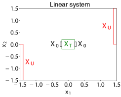
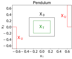
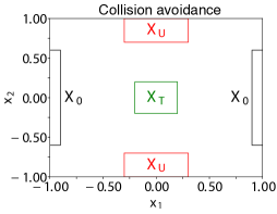
Figure 5: Reach-avoid specifications for three of the main benchmarks used for the experiments.

The Lipschitz constant w.r.t. $\mathbf{x}$ is $L_{f,\mathbf{x}}=1$ and the Lipschitz constant w.r.t. $\mathbf{u}$ is $L_{f,\mathbf{u}}=0.95$.

For all our main experiments, we use the loss function $\|\mathbf{x}\|_{2}-1=\sqrt{\mathbf{x}_{1}^{2}+\mathbf{x}_{2}^{2}}-1$ to train input policies, which is a sensible loss function since the goal states are around the origin and the unsafe states are the farthest away from the origin. When training input policies with the Stable-Baselines3 algorithms, we instead assign a loss of $5$ when entering the unsafe region and a loss of $-5$ when entering the goal region, and use the loss function $\|\mathbf{x}\|_{2}-1=\sqrt{\mathbf{x}_{1}^{2}+\mathbf{x}_{2}^{2}}-1$ otherwise.

C.1.2 Pendulum

In Pendulum (pendulum), we have $\mathcal{X}=[-0.7,0.7]^{2}\subseteq\mathbb{R}^{2}$ and $\mathcal{U}=[-1,1]\subseteq\mathbb{R}$ and $\mathcal{N}=[-1,1]^{2}\subseteq\mathbb{R}^{2}$. The system dynamics function $f\colon\mathcal{X}\times\mathcal{U}\times\mathcal{N}\to\mathcal{X}$ is given by

$$f(\mathbf{x},\mathbf{u},\omega) =\begin{pmatrix}\mathbf{x}_{1}+0.01\omega_{1}\\ 0\end{pmatrix}$$

$$+\begin{pmatrix}\delta\\ 1\end{pmatrix}\text{clip}\left((1-b)\mathbf{x}_{2}+\delta\left(\frac{-1.5G\sin(\mathbf{x}_{1}+\pi)}{2l}+\frac{6}{ml^{2}}\mathbf{u}\right)+0.02\omega_{2},-5,5\right),$$

where $\delta=0.05$, $G=10$, $m=0.15$, $l=0.5$ and $b=0.1$. The clip function is defined as $\text{clip}(x,a,b)=\min(\max(x,a),b)$.

The noise $\omega$ has two components $\omega_{1},\omega_{2}$ which are independent and have the Triangular distribution.

The initial states are $\mathcal{X}_{0}=[-0.3,0.3]^{2}$, the target states are $\mathcal{X}_{T}=[-0.2,0.2]^{2}$, and the unsafe states are $\mathcal{X}_{U}=([-0.7,-0.6]\times[-0.7,0])\cup([0.6,0.7]\times[0,0.7])$. The resulting reach-avoid task is shown in Fig. 5.

The Lipschitz constant w.r.t. $\mathbf{x}$ is $L_{f,\mathbf{x}}=1.7875$ and the Lipschitz constant w.r.t. $\mathbf{u}$ is $L_{f,\mathbf{u}}=8.4$.

For all our main experiments, we use the loss function $\mathbf{x}_{1}^{2}+0.1\mathbf{x}_{2}^{2}$ to train input policies. When training input policies with the Stable-Baselines3 algorithms, we instead assign a loss of $5$ when entering the unsafe region and a loss of $-5$ when entering the goal region, and use the loss function $\mathbf{x}_{1}^{2}+0.1\mathbf{x}_{2}^{2}$ otherwise.

C.1.3 Collision Avoidance

In Collision Avoidance (collision-avoid), we have $\mathcal{X}=[-1,1]^{2}\subseteq\mathbb{R}^{2}$, $\mathcal{U}=[-1,1]^{2}\subseteq\mathbb{R}^{2}$ and $\mathcal{N}=[-1,1]^{2}\subseteq\mathbb{R}^{2}$. The system dynamics $f\colon\mathcal{X}\times\mathcal{U}\times\mathcal{N}\to\mathcal{X}$ is given by

$$f(\mathbf{x},\mathbf{u},\omega) =\mathbf{x}+0.2\left(d_{2}\left(d_{1}\mathbf{u}+(1-d_{1})\begin{pmatrix}0\\ 1\end{pmatrix}\right)+(1-d_{2})\begin{pmatrix}0\\ -1\end{pmatrix}\right)+0.05\omega,$$

where $d_{1}=\min\left\{\dfrac{10}{3}\left\|\mathbf{x}-\begin{pmatrix}0\\ 1\end{pmatrix}\right\|_{2},1\right\}$ and $d_{2}=\min\left\{\dfrac{10}{3}\left\|\mathbf{x}-\begin{pmatrix}0\\ -1\end{pmatrix}\right\|_{2},1\right\}$.

The noise $\omega$ has two components $\omega_{1},\omega_{2}$ which are independent and have the Triangular distribution.

The initial states are $\mathcal{X}_{0}=([-1,-0.9]\cup[0.9,1])\times[-0.6,0.6]$, the target states are $\mathcal{X}_{T}=[-0.2,0.2]^{2}$, and the unsafe states are $\mathcal{X}_{U}=[-0.3,0.3]\cup([-1,-0.7]\times[0.7,1])$. The resulting reach-avoid task is shown in Fig. 5.

The Lipschitz constant w.r.t. $\mathbf{x}$ is $L_{f,\mathbf{x}}=3$ and the Lipschitz constant w.r.t. $\mathbf{u}$ is $L_{f,\mathbf{u}}=0.2$.

We use the same loss functions for training input policies as for Linear System.

C.1.4 Linear System (hard layout)

The hard layout of Linear System (linear-sys) has the same dynamics as the default version defined in Sect. C.1.1, but we modify the reach-avoid specification. Specifically, we use the reach-avoid specification with $\mathcal{X}_{0}=([-1.4,-1.3]\cup[1.3,1.4])\times[-0.1,0.1]$ and $\mathcal{X}_{U}=([-0.9,-0.7]\cup[0.7,0.9])\times[-0.2,0.2]$. The resulting reach-avoid task is shown in Fig. 4.

C.1.5 Triple Integrator

In Triple Integrator (triple-integrator), we have $\mathcal{X}=[-1,1]^{3}\subseteq\mathbb{R}^{3}$ and $\mathcal{U}=[-1,1]\subseteq\mathbb{R}$ and $\mathcal{N}=[-1,1]^{3}\subseteq\mathbb{R}^{3}$. The system dynamics function $f\colon\mathcal{X}\times\mathcal{U}\times\mathcal{N}\to\mathcal{X}$ is given by

$$f(\mathbf{x},\mathbf{u},\omega)=A\mathbf{x}+B\mathbf{u}+W\omega,$$

where $A=\begin{pmatrix}1&0.045&0\\ 0&1&0.045\\ 0&0&0.9\end{pmatrix}$ and $B=\begin{pmatrix}0.35\\ 0.45\\ 0.5\end{pmatrix}$ and $W=\begin{pmatrix}0.01&0&0\\ 0&0.01&0\\ 0&0&0.005\end{pmatrix}$.

The noise $\omega$ has three components which are independent and have the Triangular distribution.

The initial states are $\mathcal{X}_{0}=([-0.25,-0.2]^{2}\cup[0.2,0.25]^{2})\times[-0.1,0.1]$, the target states are $\mathcal{X}_{T}=[-0.2,0.2]^{3}$, and the unsafe states are $\mathcal{X}_{U}=([-1,-0.9]^{2}\times[-1,0])\cup([0.9,1]^{2}\times[0,1])$.

The Lipschitz constant w.r.t. $\mathbf{x}$ is $L_{f,\mathbf{x}}=1.045$ and the Lipschitz constant w.r.t. $\mathbf{u}$ is $L_{f,\mathbf{u}}=1.3$.

For training input policies, we use the loss function $\|\mathbf{x}\|_{2}^{2}-1=\mathbf{x}_{1}^{2}+\mathbf{x}_{2}^{2}+\mathbf{x}_{3}^{2}-1$.

C.2 Hyperparameters

number of random points	$90\,000$
number of counterexamples	$30\,000$
epochs	$25$
batch size	$4096$
counterexample fraction	$0.25$
counterexample refresh fraction	$0.5$
optimizer	Adam [43]
learning rate $V$	$5\cdot 10^{-4}$
learning rate $\pi$	$5\cdot 10^{-5}$
$N$ loss learner	16
pretraining steps (PPO)	$10^{6}$
points init. verification grid	$10^{6}$
max refine factor $C$	$10$
noise partition cells	$144$

Table 1: Hyperparameters common for all benchmarks.

model	lin.sys	pendulum	coll.avoid	lin.sys (hard)	triple int.
loss mesh $\tau$	$0.1(1{-}\rho)$	$0.002(1{-}\rho)$	$0.01(1{-}\rho)$	$0.001(1{-}\rho)$	$0.02(1{-}\rho)$
max. loss mesh $\tau$	$10^{-4}$	$10^{-4}$	0	0	0.002
min. $L_{\pi}$ pretrain	3	3	10	3	3
min. $L_{\pi}$ loss learner	0.5	0.1	5	1	0

Table 2: Benchmark-specific hyperparameters.

In this appendix, we give an overview of the hyperparameters of our algorithm. Tables 1 and 2 report the hyperparameters. We now discuss the meaning of these parameters, the reason why we have chosen them, and the extent to which we have done hyperparameter tuning.

C.2.1 Hyperparameters for all benchmarks

We first discuss the hyperparameters common for all benchmarks.

Samples and buffers    Recall from Sect. A.4 that the loss function of the learner is divided into ‘random’ points and counterexamples. For efficiency reasons, our implementation keeps track of a buffer for both types of points and samples from these buffers when needed. We use a buffer of size $90\,000$ for the random points and a buffer of size $30\,000$ for the counterexamples. The number of epochs is the number of full passes made over these buffers in a single learner iteration. Within each epoch, the data is divided into batches of $4\,096$ points, and the counterexample fraction (we use $0.25$) gives the fraction of counterexamples in each batch. After each verifier iteration, a part of the counterexamples in the counterexample buffer is replaced by new counterexamples. The counterexample refresh fraction (we use $0.5$) gives the fraction of the counterexample buffer that is replaced with new counterexamples. We did not tune these hyperparameters for our experiments.

Optimizer and learning rate    We take the optimizer, learning rates for $V$ and $\pi$ from [73] and have not performed any tuning on them. We also take the number of samples $N$ used in the expected decrease terms in the loss function of the learner (see Sect. A.4) from [73].

PPO training    The number of steps for training input policies with PPO is $10^{6}$. We observed that this number of steps leads to adequate convergence of the policies; however, we did not perform more sophisticated tuning of the number of training steps.

Verifier grid    Using $10^{6}$ points for the initial verification grid seems to give a good balance between the total time spent by the learner and the verifier; we briefly experimented with a smaller number of points on linear-sys (which gave inferior results).

Refinement    We set the maximum refinement factor $C$ to 10, which seems to yield a good balance between (a) not having to refine too often and (b) not wasting too much time when hard violations are found after the first local refinement.

Noise partition    Finally, we take the number of noise partition cells of $12^{2}=144$ used for computing upper bounds on expectations from [73].

C.2.2 Benchmark-specific hyperparameters

We now discuss the benchmark-specific hyperparameters, which can be divided into two categories.

Loss mesh    The main benchmark-specific parameter is the loss mesh. Recall from Sect. A.4 that this loss mesh is contained in the loss function of the learner and is different from the mesh used by the verifier. Intuitively, when the loss function is trained to zero for a particular loss mesh $\tau$, then a discretization of this same mesh $\tau$ in the verifier should suffice to successfully verify the certificate $V$. In practice, the loss function is not trained to zero exactly, so we expect that the loss mesh should be higher than the (worst-case) mesh needed by the verifier.

We observed that good values for the loss mesh are proportional to $1-\rho$, which yields a $\tau K$ that is approximately constant since $K$ is typically approximately proportional to $\frac{1}{1-\rho}$. Based on this observation, we tuned the loss mesh on each benchmark on one relatively low probability bound (99.9% for linear-sys, 90% for the other benchmarks). When going to lower probabilities, we observed that performance sometimes deteriorated when setting the loss mesh too high, leading to higher training times. (The reason for this appeared to be that the ‘$K$ is proportional to $\frac{1}{1-\rho}$’ approximation only works for $\rho$ sufficiently close to 1). For this reason, we also have a maximum value for the loss mesh. On the other hand, for the baseline and the verifier where local refinement is disabled (w/o local), we did not use this maximum value as taking the value from the formula gave better results (due to lower verification times).

Minimum Lipschitz constants    The loss function used in PPO pretraining includes an extra term that gives a loss if the Lipschitz constant of the policy is larger than a prespecified value. We set this value to 3. For collision-avoid, we observed (for low probabilities) that the final learned policy often had a Lipschitz constant larger than 3. Therefore, we set the minimum Lipschitz constant to a higher value for collision-avoid. Finally, we use a lower bound on $L_{\pi}$ as it is used in the loss function of the learner, to prevent the learner from finding local optima where the policy has a very small Lipschitz constant. We selected the size of this minimum primarily based on the size of $L_{f,\mathbf{u}}$ compared to $L_{f,\mathbf{x}}$: if $L_{f,\mathbf{u}}$ is small compared to $L_{f,\mathbf{x}}$, then we can afford a much larger $L_{\pi}$ without this having a large effect on the overall Lipschitz constant $K$.

C.2.3 Hyperparameters for Triple Integrator

Finally, we note that for the 3D benchmark triple-integrator, we have selected a number of hyperparameters differently. We have increased the number of noise partition cells to $6^{3}=216$. To keep the overall time used by the verifier manageable, we have decreased the number of points in the initial verification grid to $77^{3}=456\,533$. We also decreased the maximum refinement factor $C$ to 4. Finally, rather than sampling random points (for the buffer used in the loss function) for each of the conditions proportional to the area of the respective region (e.g., the initial state or unsafe region), we selected at least 10% of the points for each region.

Appendix D Further Empirical Results

In this appendix, we provide more detailed results for the experiments presented in Sect. 6 and perform additional experiments.

(a) Linear system.

(b) Pendulum.

(c) Collision avoidance.

Figure 6: Run times for all verifier variants, using policy and certificate networks of $2$ hidden layers (averages over 5 seeds; error bars showing standard deviations) for reach-avoid tasks with different probability bounds $\rho$, using a timeout of 1 hour.

D.1 Results for different neural network sizes

For the experiments in Sect. 6, we used policy and certificate networks that both consist of hidden 3 layers of 128 neurons each. To test the effect of reducing the network sizes, we consider the same experiment as in Fig. 2, but now for policy and certificate networks with 2 hidden layers (of 128 neurons each). We only consider the baseline verifier (with all our contributions from Sects. 4 and 5 disabled) and our new method (which has all our contributions enabled). We omit the intermediate verifiers (with only part of our contributions enabled) for brevity.

The average run times until termination of the learner-verifier framework are presented in Fig. 6 (we use the same criteria for failed runs as described in Sect. 6). We observe that the average run times when using networks of 2 hidden layers are substantially higher than for networks of 3 hidden layers (see Fig. 2). This performance difference is especially apparent for collision-avoid with $\rho=98\%$: using 3 hidden layers, the average run time is $461\text{\,}\mathrm{s}$, whereas with 2 hidden layers, our method is unable to verify the policy within the timeout of 1 hour. Since we observe that our method performs better when using networks of 3 hidden layers, we use these sizes for the policy and certificate networks in the experiments presented in Sect. 6.

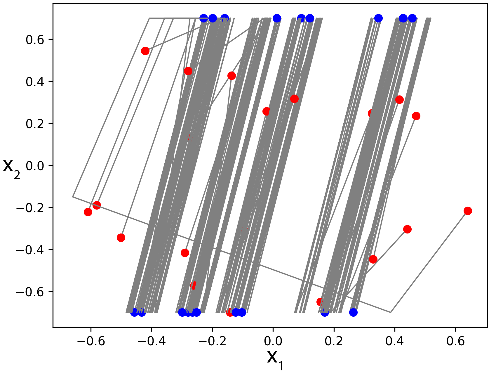
(a) Policy trained with A2C (for $10^{4}$ steps).

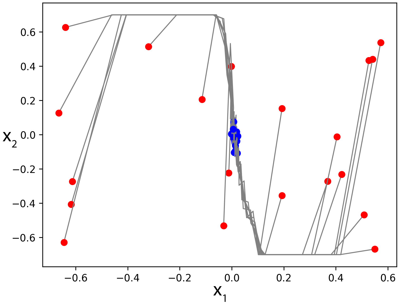
(b) Policy trained with TRPO (for $10^{4}$ steps).

Figure 7: Simulated executions of pendulum with policies trained with A2C and TRPO.

D.2 Results for Stable-Baselines policies

We zoom in on the results shown in Fig. 3 for the A2C algorithm on the pendulum benchmarks. Recall from Fig. 3 presented in the empirical evaluation that our method failed to verify this benchmark when the policy is trained using A2C for $10^{4}$ or $10^{5}$ steps. By contrast, the other algorithms (SAC, TQC, and TRPO) did lead to our method being able to verify the policy. To investigate this discrepancy, we present in Fig. 7 simulated executions (from random initial states) of the input policies trained for $10^{4}$ steps with A2C and TRPO. The executions under the TRPO policy converge to the target region $\mathcal{X}_{T}=[-0.2,0.2]^{2}$, whereas the executions under the A2C policy fail to reach the target. This result confirms that our method’s poor performance on the A2C policies was due to input policies of bad quality. In this case, training the A2C policy for more steps (e.g., $10^{6}$) mitigates these issues, as also shown by the results in Fig. 3.

D.3 Comparison against LipBaB

setting	network	$L_{\text{Ours}}$	$L_{\text{LipBaB},1}$	$L_{\text{LipBaB}}$	lower	$t_{\text{better}}$	$t_{\text{exact}}$
2 layers, $\rho=0.99$	$\pi$	2.40	2.70	1.84	1.84	46.8	316
3 layers, $\rho=0.99$	$\pi$	2.82	3.66	2.08	1.95	153.2	>600
2 layers, $\rho=0.99995$	$\pi$	0.54	0.62	0.44	0.44	27.7	190
3 layers, $\rho=0.99995$	$\pi$	0.69	0.89	0.48	0.47	90.4	>474
2 layers, $\rho=0.99$	$V$	131.9	134.4	92.1	92.1	3.8	469
3 layers, $\rho=0.99$	$V$	225.9	333.8	225.0	90.6	>565.9	>600
2 layers, $\rho=0.99995$	$V$	20497	19596	18722	18722	0.4	51
3 layers, $\rho=0.99995$	$V$	24607	24027	19924	19909	2.6	>492

Table 3: Lipschitz constants and timings for LipBaB in comparison to our method, averaged over 5 seeds, for the policy network ($\pi$) and the certificate network ($V$), in different settings for linear-sys. For LipBaB, we used a timeout of 600 seconds.

We compare our method for computing Lipschitz constants to another method for computing global Lipschitz constants, called LipBaB [16]. We consider the final networks returned upon termination of the learner-verifier framework (using our method). We then compute the Lipschitz constant for the policy network and the certificate network using both our method and LipBaB. We note that LipBaB is an anytime algorithm.

Table 3 shows results for Lipschitz computations using LipBaB, in comparison to our method (using both weighted norms (Sect. 4.1) and averaged activation operators (Sect. A.1)). All tested networks were trained for the linear-sys benchmark. The first two columns specify the network we trained on by specifying the number of layers, probability bound $\rho$, and whether we consider the policy network ($\pi$) or the certificate network ($V$). The next column gives the Lipschitz constant computed using our method. For each setting, our method takes 0.2 seconds for the first call (due to JIT compilation by JAX) and 0.0002 seconds (0.2 milliseconds) for subsequent calls (if the code is already JIT-compiled). The column titled ‘$L_{\text{LipBaB},1}$’ gives the first result computed by LipBaB. Computing this first result takes 0.4 seconds for 2 layers and 0.8 seconds for 3 layers. The next two columns (titled ‘$L_{\text{LipBaB}}$’ and ‘lower’) provide the final Lipschitz constant computed by LipBaB upon termination or after 600 seconds (whichever occurs first). The column titled $t_{\text{better}}$ gives the first time after which LipBaB has computed a better Lipschitz constant than our method. The final column, titled $t_{\text{exact}}$, gives the time until LipBaB returns the exact Lipschitz constant (counting a timeout as 600 seconds, and an inequality sign indicating that in at least one run the exact Lipschitz constant was not found in 600 seconds). Finally, we note that for 3 layers, $\rho=0.99$, and the certificate network ($V$), LipBaB was not able to compute a better Lipschitz constant than our method within 600 seconds on 3 out of 5 seeds.

From the results, we see that the lower probability bound ($\rho=0.99$) is generally harder for LipBaB than the high probability bound ($\rho=0.99995$). Moreover, networks with 3 layers are, in general, harder than networks with 2 layers.

benchmark	$\rho$	run time [s]	st.dev. [s]	# points local	# points w/o local
linear-sys	0.8	598	78	$2.70\text{\times}{10}^{07}$	$1.82\text{\times}{10}^{10}$
linear-sys	0.9	1558	432	$1.51\text{\times}{10}^{08}$	$2.67\text{\times}{10}^{10}$
linear-sys	0.95	3600 (TO)	NaN	$5.74\text{\times}{10}^{08}$	$3.35\text{\times}{10}^{10}$
triple-integrator	0.8	859	187	$1.20\text{\times}{10}^{08}$	$7.12\text{\times}{10}^{13}$
triple-integrator	0.9	1554	551	$1.42\text{\times}{10}^{08}$	$1.31\text{\times}{10}^{13}$
triple-integrator	0.95	2290	857	$3.16\text{\times}{10}^{08}$	$7.01\text{\times}{10}^{13}$

Table 4: Average run times for linear-sys (with the difficult reach-avoid specification) and triple-integrator, as well as the total number of samples used by the verifier using our method (with local refinements), versus the verifier without local refinements.

D.4 Results for triple integrator and linear system (difficult layout)

We provide further results for the linear-sys (with the difficult reach-avoid specification) and triple-integrator benchmarks. For both benchmarks, we apply our method to solve Problem 1 for different values of $\rho$. The resulting average run times (over 5 random seeds) are presented in Table 4 (we use the same criteria for failed runs as described in Sect. 6). For linear-sys with $\rho=95\%$, our method could solve Problem 1 only for 2 out of the 5 seeds (and was thus considered as failed). For all other instances, our method was able to solve Problem 1 on all 5 seeds.

Table 4 also presents the total number of discretized points needed by the verifier in the final iteration of the learner-verifier framework. To illustrate the effectiveness of our local refinement scheme from Sect. 5, we also compute the total number of points that would be needed by a verifier that uses a uniform discretization (instead of our local refinements). We obtain the latter value based on the smallest mesh used in our local refinement scheme, which we use to compute the number of points that a uniform discretization of this mesh size consists of. Table 4 shows that our local refinement scheme reduces the total number of points needed by the verifier by several orders of magnitude.

References

- Abate et al. [2021a] Alessandro Abate, Daniele Ahmed, Alec Edwards, Mirco Giacobbe, and Andrea Peruffo. FOSSIL: a software tool for the formal synthesis of Lyapunov functions and barrier certificates using neural networks. In HSCC, pages 24:1–24:11. ACM, 2021a.
- Abate et al. [2021b] Alessandro Abate, Daniele Ahmed, Mirco Giacobbe, and Andrea Peruffo. Formal synthesis of Lyapunov neural networks. IEEE Control. Syst. Lett., 5(3):773–778, 2021b.
- Abate et al. [2021c] Alessandro Abate, Mirco Giacobbe, and Diptarko Roy. Learning probabilistic termination proofs. In CAV (2), volume 12760 of Lecture Notes in Computer Science, pages 3–26. Springer, 2021c.
- Abate et al. [2023] Alessandro Abate, Alec Edwards, Mirco Giacobbe, Hashan Punchihewa, and Diptarko Roy. Quantitative verification with neural networks. In CONCUR, volume 279 of LIPIcs, pages 22:1–22:18. Schloss Dagstuhl - Leibniz-Zentrum für Informatik, 2023.
- Achiam et al. [2017] Joshua Achiam, David Held, Aviv Tamar, and Pieter Abbeel. Constrained policy optimization. In ICML, volume 70 of Proceedings of Machine Learning Research, pages 22–31. PMLR, 2017.
- Agrawal et al. [2018] Sheshansh Agrawal, Krishnendu Chatterjee, and Petr Novotný. Lexicographic ranking supermartingales: an efficient approach to termination of probabilistic programs. Proc. ACM Program. Lang., 2(POPL):34:1–34:32, 2018.
- Alshiekh et al. [2018] Mohammed Alshiekh, Roderick Bloem, Rüdiger Ehlers, Bettina Könighofer, Scott Niekum, and Ufuk Topcu. Safe reinforcement learning via shielding. In AAAI, pages 2669–2678. AAAI Press, 2018.
- Altman [2021] Eitan Altman. Constrained Markov decision processes. Routledge, 2021.
- Ames et al. [2017] Aaron D. Ames, Xiangru Xu, Jessy W. Grizzle, and Paulo Tabuada. Control barrier function based quadratic programs for safety critical systems. IEEE Trans. Autom. Control., 62(8):3861–3876, 2017.
- Amodei et al. [2016] Dario Amodei, Chris Olah, Jacob Steinhardt, Paul F. Christiano, John Schulman, and Dan Mané. Concrete problems in AI safety. CoRR, abs/1606.06565, 2016.
- Avant and Morgansen [2023] Trevor Avant and Kristi A. Morgansen. Analytical bounds on the local Lipschitz constants of ReLU networks. IEEE Transactions on Neural Networks and Learning Systems, 2023.
- Badings et al. [2023] Thom S. Badings, Licio Romao, Alessandro Abate, David Parker, Hasan A. Poonawala, Mariëlle Stoelinga, and Nils Jansen. Robust control for dynamical systems with non-gaussian noise via formal abstractions. J. Artif. Intell. Res., 76:341–391, 2023.
- Baillon et al. [1978] Jean-Bernard Baillon, Ronald E. Bruck, and Simeon Reich. On the asymptotic behavior of nonexpansive mappings and semigroups in banach spaces. Houston J. Math., 4:1–9, 1978.
- Berkenkamp et al. [2017] Felix Berkenkamp, Matteo Turchetta, Angela P. Schoellig, and Andreas Krause. Safe model-based reinforcement learning with stability guarantees. In NIPS, pages 908–918, 2017.
- Bertsekas and Shreve [1978] Dimitri P. Bertsekas and Steven E. Shreve. Stochastic Optimal Control: The Discrete-time Case. Athena Scientific, 1978. ISBN 1-886529-03-5.
- Bhowmick et al. [2021] Aritra Bhowmick, Meenakshi D’Souza, and G. Srinivasa Raghavan. LipBaB: Computing exact Lipschitz constant of ReLU networks. In ICANN (4), volume 12894 of Lecture Notes in Computer Science, pages 151–162. Springer, 2021.
- Biggio et al. [2013] Battista Biggio, Igino Corona, Davide Maiorca, Blaine Nelson, Nedim Srndic, Pavel Laskov, Giorgio Giacinto, and Fabio Roli. Evasion attacks against machine learning at test time. In ECML/PKDD (3), volume 8190 of Lecture Notes in Computer Science, pages 387–402. Springer, 2013.
- Bradbury et al. [2018] James Bradbury, Roy Frostig, Peter Hawkins, Matthew James Johnson, Chris Leary, Dougal Maclaurin, George Necula, Adam Paszke, Jake VanderPlas, Skye Wanderman-Milne, and Qiao Zhang. JAX: composable transformations of Python+NumPy programs, 2018. URL http://github.com/google/jax.
- Brunke et al. [2022] Lukas Brunke, Melissa Greeff, Adam W. Hall, Zhaocong Yuan, Siqi Zhou, Jacopo Panerati, and Angela P. Schoellig. Safe learning in robotics: From learning-based control to safe reinforcement learning. Annu. Rev. Control. Robotics Auton. Syst., 5:411–444, 2022.
- Bungert et al. [2021] Leon Bungert, René Raab, Tim Roith, Leo Schwinn, and Daniel Tenbrinck. CLIP: cheap Lipschitz training of neural networks. In SSVM, volume 12679 of Lecture Notes in Computer Science, pages 307–319. Springer, 2021.
- Busoniu et al. [2018] Lucian Busoniu, Tim de Bruin, Domagoj Tolic, Jens Kober, and Ivana Palunko. Reinforcement learning for control: Performance, stability, and deep approximators. Annu. Rev. Control., 46:8–28, 2018.
- Chakarov and Sankaranarayanan [2013] Aleksandar Chakarov and Sriram Sankaranarayanan. Probabilistic program analysis with martingales. In CAV, volume 8044 of Lecture Notes in Computer Science, pages 511–526. Springer, 2013.
- Chang et al. [2019] Ya-Chien Chang, Nima Roohi, and Sicun Gao. Neural Lyapunov control. In NeurIPS, pages 3240–3249, 2019.
- Chatterjee et al. [2017] Krishnendu Chatterjee, Petr Novotný, and Dorde Zikelic. Stochastic invariants for probabilistic termination. In POPL, pages 145–160. ACM, 2017.
- Choi et al. [2020] Jason J. Choi, Fernando Castañeda, Claire J. Tomlin, and Koushil Sreenath. Reinforcement learning for safety-critical control under model uncertainty, using control Lyapunov functions and control barrier functions. In Robotics: Science and Systems, 2020.
- Clark [2021] Andrew Clark. Control barrier functions for stochastic systems. Autom., 130:109688, 2021.
- Combettes and Pesquet [2020] Patrick L. Combettes and Jean-Christophe Pesquet. Lipschitz certificates for layered network structures driven by averaged activation operators. SIAM Journal on Mathematics of Data Science, 2(2):529–557, 2020.
- Dawson et al. [2023] Charles Dawson, Sicun Gao, and Chuchu Fan. Safe control with learned certificates: A survey of neural Lyapunov, barrier, and contraction methods for robotics and control. IEEE Trans. Robotics, 39(3):1749–1767, 2023.
- De Queiroz et al. [2000] Marcio S. De Queiroz, Darren M. Dawson, Siddharth P. Nagarkatti, and Fumin Zhang. Lyapunov-based control of mechanical systems. Springer Science & Business Media, 2000.
- Duan et al. [2016] Yan Duan, Xi Chen, Rein Houthooft, John Schulman, and Pieter Abbeel. Benchmarking deep reinforcement learning for continuous control. In ICML, volume 48 of JMLR Workshop and Conference Proceedings, pages 1329–1338. JMLR.org, 2016.
- Durrett [1996] Richard Durrett. Stochastic Calculus: A Practical Introduction. CRC Press, 1st edition, 1996.
- Fazlyab et al. [2019] Mahyar Fazlyab, Alexander Robey, Hamed Hassani, Manfred Morari, and George J. Pappas. Efficient and accurate estimation of Lipschitz constants for deep neural networks. In NeurIPS, pages 11423–11434, 2019.
- García and Fernández [2015] Javier García and Fernando Fernández. A comprehensive survey on safe reinforcement learning. J. Mach. Learn. Res., 16:1437–1480, 2015.
- Gómez et al. [2020] Fabian Latorre Gómez, Paul Rolland, and Volkan Cevher. Lipschitz constant estimation of neural networks via sparse polynomial optimization. In ICLR. OpenReview.net, 2020.
- Gouk et al. [2021] Henry Gouk, Eibe Frank, Bernhard Pfahringer, and Michael J. Cree. Regularisation of neural networks by enforcing Lipschitz continuity. Mach. Learn., 110(2):393–416, 2021.
- Gowal et al. [2018] Sven Gowal, Krishnamurthy Dvijotham, Robert Stanforth, Rudy Bunel, Chongli Qin, Jonathan Uesato, Relja Arandjelovic, Timothy A. Mann, and Pushmeet Kohli. On the effectiveness of interval bound propagation for training verifiably robust models. CoRR, abs/1810.12715, 2018.
- Huang et al. [2017] Xiaowei Huang, Marta Kwiatkowska, Sen Wang, and Min Wu. Safety verification of deep neural networks. In CAV (1), volume 10426 of Lecture Notes in Computer Science, pages 3–29. Springer, 2017.
- Huang et al. [2020] Xiaowei Huang, Daniel Kroening, Wenjie Ruan, James Sharp, Youcheng Sun, Emese Thamo, Min Wu, and Xinping Yi. A survey of safety and trustworthiness of deep neural networks: Verification, testing, adversarial attack and defence, and interpretability. Comput. Sci. Rev., 37:100270, 2020.
- Jagtap et al. [2021] Pushpak Jagtap, Sadegh Soudjani, and Majid Zamani. Formal synthesis of stochastic systems via control barrier certificates. IEEE Trans. Autom. Control., 66(7):3097–3110, 2021.
- Jordan and Dimakis [2020] Matt Jordan and Alexandros G. Dimakis. Exactly computing the local Lipschitz constant of ReLU networks. In NeurIPS, 2020.
- Katz et al. [2017] Guy Katz, Clark Barrett, David L Dill, Kyle Julian, and Mykel J Kochenderfer. Reluplex: An efficient SMT solver for verifying deep neural networks. In Computer Aided Verification, volume 29, pages 97–117. Springer, 2017.
- Khalil and Grizzle [2002] Hassan K Khalil and Jessy W Grizzle. Nonlinear systems, volume 3. Prentice hall Upper Saddle River, NJ, 2002.
- Kingma and Ba [2015] Diederik P. Kingma and Jimmy Ba. Adam: A method for stochastic optimization. In ICLR (Poster), 2015.
- Kurakin et al. [2017] Alexey Kurakin, Ian J. Goodfellow, and Samy Bengio. Adversarial examples in the physical world. In ICLR (Workshop). OpenReview.net, 2017.
- Lahijanian et al. [2015] Morteza Lahijanian, Sean B. Andersson, and Calin Belta. Formal verification and synthesis for discrete-time stochastic systems. IEEE Trans. Autom. Control., 60(8):2031–2045, 2015.
- Lavaei et al. [2022] Abolfazl Lavaei, Sadegh Soudjani, Alessandro Abate, and Majid Zamani. Automated verification and synthesis of stochastic hybrid systems: A survey. Autom., 146:110617, 2022.
- Lechner et al. [2022] Mathias Lechner, Dorde Zikelic, Krishnendu Chatterjee, and Thomas A. Henzinger. Stability verification in stochastic control systems via neural network supermartingales. In AAAI, pages 7326–7336. AAAI Press, 2022.
- Lillicrap et al. [2016] Timothy P. Lillicrap, Jonathan J. Hunt, Alexander Pritzel, Nicolas Heess, Tom Erez, Yuval Tassa, David Silver, and Daan Wierstra. Continuous control with deep reinforcement learning. In ICLR (Poster), 2016.
- Lindemann and Dimarogonas [2019] Lars Lindemann and Dimos V. Dimarogonas. Control barrier functions for signal temporal logic tasks. IEEE Control. Syst. Lett., 3(1):96–101, 2019.
- Mathiesen et al. [2023] Frederik Baymler Mathiesen, Simeon C. Calvert, and Luca Laurenti. Safety certification for stochastic systems via neural barrier functions. IEEE Control. Syst. Lett., 7:973–978, 2023.
- Meng and Liu [2022] Yiming Meng and Jun Liu. Sufficient conditions for robust probabilistic reach-avoid-stay specifications using stochastic Lyapunov-barrier functions. In ACC, pages 2283–2288. IEEE, 2022.
- Pauli et al. [2022] Patricia Pauli, Anne Koch, Julian Berberich, Paul Kohler, and Frank Allgöwer. Training robust neural networks using Lipschitz bounds. IEEE Control. Syst. Lett., 6:121–126, 2022.
- Prajna et al. [2007] Stephen Prajna, Ali Jadbabaie, and George J. Pappas. A framework for worst-case and stochastic safety verification using barrier certificates. IEEE Trans. Autom. Control., 52(8):1415–1428, 2007.
- Puterman [1994] Martin L. Puterman. Markov Decision Processes: Discrete Stochastic Dynamic Programming. Wiley Series in Probability and Statistics. Wiley, 1994.
- Raffin et al. [2021] Antonin Raffin, Ashley Hill, Adam Gleave, Anssi Kanervisto, Maximilian Ernestus, and Noah Dormann. Stable-baselines3: Reliable reinforcement learning implementations. J. Mach. Learn. Res., 22:268:1–268:8, 2021.
- Recht [2019] Benjamin Recht. A tour of reinforcement learning: The view from continuous control. Annu. Rev. Control. Robotics Auton. Syst., 2:253–279, 2019.
- Richards et al. [2018] Spencer M. Richards, Felix Berkenkamp, and Andreas Krause. The Lyapunov neural network: Adaptive stability certification for safe learning of dynamical systems. In CoRL, volume 87 of Proceedings of Machine Learning Research, pages 466–476. PMLR, 2018.
- Santoyo et al. [2021] Cesar Santoyo, Maxence Dutreix, and Samuel Coogan. A barrier function approach to finite-time stochastic system verification and control. Autom., 125:109439, 2021.
- Schulman et al. [2017] John Schulman, Filip Wolski, Prafulla Dhariwal, Alec Radford, and Oleg Klimov. Proximal policy optimization algorithms. CoRR, abs/1707.06347, 2017.
- Shi et al. [2022] Zhouxing Shi, Yihan Wang, Huan Zhang, J. Zico Kolter, and Cho-Jui Hsieh. Efficiently computing local Lipschitz constants of neural networks via bound propagation. In NeurIPS, 2022.
- Steinhardt and Tedrake [2011] Jacob Steinhardt and Russ Tedrake. Finite-time regional verification of stochastic nonlinear systems. In Robotics: Science and Systems, 2011.
- Summers and Lygeros [2010] Sean Summers and John Lygeros. Verification of discrete time stochastic hybrid systems: A stochastic reach-avoid decision problem. Autom., 46(12):1951–1961, 2010.
- Szegedy et al. [2014] Christian Szegedy, Wojciech Zaremba, Ilya Sutskever, Joan Bruna, Dumitru Erhan, Ian J. Goodfellow, and Rob Fergus. Intriguing properties of neural networks. In ICLR (Poster), 2014.
- Takisaka et al. [2021] Toru Takisaka, Yuichiro Oyabu, Natsuki Urabe, and Ichiro Hasuo. Ranking and repulsing supermartingales for reachability in randomized programs. ACM Trans. Program. Lang. Syst., 43(2):5:1–5:46, 2021.
- Virmaux and Scaman [2018] Aladin Virmaux and Kevin Scaman. Lipschitz regularity of deep neural networks: analysis and efficient estimation. In NeurIPS, pages 3839–3848, 2018.
- Weng et al. [2018] Tsui-Wei Weng, Huan Zhang, Hongge Chen, Zhao Song, Cho-Jui Hsieh, Luca Daniel, Duane S. Boning, and Inderjit S. Dhillon. Towards fast computation of certified robustness for ReLU networks. In ICML, volume 80 of Proceedings of Machine Learning Research, pages 5273–5282. PMLR, 2018.
- Williams [1991] David Williams. Probability with Martingales. Cambridge mathematical textbooks. Cambridge University Press, 1991.
- Wu et al. [2023] Junlin Wu, Andrew Clark, Yiannis Kantaros, and Yevgeniy Vorobeychik. Neural Lyapunov control for discrete-time systems. In NeurIPS, 2023.
- Xiao and Belta [2022] Wei Xiao and Calin Belta. High-order control barrier functions. IEEE Trans. Autom. Control., 67(7):3655–3662, 2022.
- Zamani et al. [2014] Majid Zamani, Peyman Mohajerin Esfahani, Rupak Majumdar, Alessandro Abate, and John Lygeros. Symbolic control of stochastic systems via approximately bisimilar finite abstractions. IEEE Trans. Autom. Control., 59(12):3135–3150, 2014.
- Zhang et al. [2019] Huan Zhang, Pengchuan Zhang, and Cho-Jui Hsieh. Recurjac: An efficient recursive algorithm for bounding jacobian matrix of neural networks and its applications. In AAAI, pages 5757–5764. AAAI Press, 2019.
- Zhou et al. [2022] Ruikun Zhou, Thanin Quartz, Hans De Sterck, and Jun Liu. Neural Lyapunov control of unknown nonlinear systems with stability guarantees. In NeurIPS, 2022.
- Zikelic et al. [2023a] Dorde Zikelic, Mathias Lechner, Thomas A. Henzinger, and Krishnendu Chatterjee. Learning control policies for stochastic systems with reach-avoid guarantees. In AAAI, pages 11926–11935. AAAI Press, 2023a.
- Zikelic et al. [2023b] Dorde Zikelic, Mathias Lechner, Abhinav Verma, Krishnendu Chatterjee, and Thomas A. Henzinger. Compositional policy learning in stochastic control systems with formal guarantees. In NeurIPS, 2023b.
- Zühlke and Kudenko [2024] Monty-Maximilian Zühlke and Daniel Kudenko. Adversarial robustness of neural networks from the perspective of Lipschitz calculus: A survey. ACM Computing Surveys, 2024.