Quark orbital angular momentum in the proton from a twist-3 generalized parton distribution

Abstract

Quark orbital angular momentum in the proton is evaluated via a Lattice QCD calculation of the second Mellin moment of the twist-3 generalized parton distribution $\widetilde{E}_{2T}$ in the forward limit. The connection between this approach to quark orbital angular momentum and approaches previously utilized in Lattice QCD calculations, via generalized transverse momentum-dependent parton distributions and via Ji’s sum rule, is reviewed. This connection can be given in terms of Lorentz invariance and equation of motion relations. The calculation of the second Mellin moment of $\widetilde{E}_{2T}$ proceeds via a finite-momentum proton matrix element of a quark bilocal operator with a straight-line gauge connection and separation in both the longitudinal and transverse directions. The dependence on the former component serves to extract the second Mellin moment, whereas the dependence on the latter component provides a transverse momentum cutoff for the matrix element. Furthermore, a derivative of the matrix element with respect to momentum transfer in the forward limit is required, which is obtained using a direct derivative method. The calculation utilizes a clover fermion ensemble at pion mass $317\,\mbox{MeV}$. The resulting quark orbital angular momentum is consistent with previous evaluations through alternative approaches, albeit with greater statistical uncertainty using a comparable number of samples.

1 Introduction

The orbital angular momentum carried by quarks inside the proton constitutes one of the pieces of the proton spin puzzle – the question of how the spin of the proton is composed of the spins and orbital angular momenta of its quark and gluon constituents. This question has prompted enduring efforts in hadronic physics, sparked by the initial EMC experiments [1, 2] that revealed that one cannot simply explain proton spin in terms of valence quark spin.

The objective of quantifying quark orbital angular momentum already meets challenges at the conceptual level as a consequence of gauge invariance, which prevents one from unambiguously separating the quark and gluon degrees of freedom. Quark fields are intrinsically linked to gluon fields, and consequently any construction of quark orbital angular momentum includes gluonic effects. The partition of orbital angular momentum in the proton into a quark and a gluon contribution is therefore a matter of definition. Whereas, in principle, a continuum of definitions is possible, two stand out prominently in discussions of the proton spin puzzle, namely, the Ji definition [3] and the Jaffe-Manohar definition [4, 5].

The quark-gluon structure of hadrons is encoded in parton distribution functions – generalized parton distributions (GPDs), revealing transverse position structure along with longitudinal momentum structure; transverse momentum-dependent parton distributions (TMDs), revealing transverse momentum structure along with longitudinal momentum structure; and, overarching the aforementioned, generalized TMDs (GTMDs), which contain GPDs and TMDs as limits. In particular, GTMDs furnish mixed transverse position and momentum information, and are therefore suited for a direct partonic definition of longitudinal orbital angular momentum [6].

Altogether, three avenues to evaluate longitudinal quark orbital angular momentum in a longitudinally polarized proton from its parton distribution functions have been constructed:

• Ji’s sum rule: The total longitudinal quark angular momentum can be derived from the quark GPD combination $H+E$ [3], whereas the longitudinal quark spin is given by the quark GPD $\widetilde{H}$. One can thus obtain the longitudinal orbital angular momentum indirectly, by taking the difference (denoting the longitudinal direction as the 3-direction),

  $$L_{3}=J_{3}-S_{3}=\frac{1}{2}\int dx\,x(H+E)-\frac{1}{2}\int dx\,\widetilde{H}\ ,$$ (1)

  where $x$ denotes the quark momentum fraction and all GPDs are evaluated in the forward limit. This relation yields specifically the orbital angular momentum according to the Ji definition.

• Twist-2 GTMD $F_{14}$: As already mentioned above, direct access to longitudinal quark orbital angular momentum can be obtained through a GTMD [6], named $F_{14}$ in the nomenclature of [7],

  $$L_{3}=-\int dx\int d^{2}k_{T}\ \frac{k_{T}^{2}}{M^{2}}\,F_{14}\ \ ,$$ (2)

  where $k_{T}$ denotes the quark transverse momentum and the GTMD is again evaluated in the forward limit. This approach allows one to evaluate quark orbital angular momentum according to both the Ji and the Jaffe-Manohar definitions (and, more generally, a continuous interpolation between the two), since the QCD matrix element definition of $F_{14}$ is based on a bilocal quark operator including a transverse separation, which allows for a choice of the shape of the gauge connection between the quark operators. A staple-shaped gauge connection path, as used in the standard definition of TMDs, yields Jaffe-Manohar quark orbital angular momentum [5, 8]; a straight-line path yields Ji quark orbital angular momentum [9, 8, 10].

• Twist-3 GPD $\widetilde{E}_{2T}$: A third way to access quark orbital angular momentum specifically according to the Ji definition is through a twist-3 GPD, named $\widetilde{E}_{2T}$ in the nomenclature of [7]. $\widetilde{E}_{2T}$ is related to the combination of orbital angular momentum and spin $L_{3}+2S_{3}$ [11, 10, 12], and one can thus obtain $L_{3}$ by subtracting twice the spin $S_{3}$,

  $$L_{3}=(L_{3}+2S_{3})-2S_{3}=-\int dx\,x\widetilde{E}_{2T}-\int dx\,\widetilde{H}\ ,$$ (3)

  where again all GPDs are evaluated in the forward limit. It should be noted that a version of this approach was first advanced by M. Polyakov and collaborators [13, 14], denoting the relevant twist-3 GPD variously as $G_{3}$ or $G_{2}$; these are related to $\widetilde{E}_{2T}$ [11]. The connection of these GPDs to quark orbital angular momentum was established using the operator product expansion. Further discussion was given in [15]. Below, an alternative approach based on GTMDs that connects (3) to (2) [10, 12] will be reviewed.

Both the expressions (1) and (2) have been employed previously to evaluate quark orbital angular momentum in the proton within Lattice QCD. Ji’s sum rule is the traditional approach that has been taken in numerous studies, cf., e.g., [16, 17, 18, 19, 20, 21, 22]. On the other hand, the approach via the GTMD $F_{14}$ was used to extend the treatment from Ji to Jaffe-Manohar quark orbital angular momentum in [23, 27], with consistency of the results for Ji quark orbital angular momentum obtained via either (1) or (2) demonstrated in [27]. In the present investigation, the third approach, via (3), is explored. After elucidating the connection between (3) and (2) in the next section, the setup and realization of a lattice calculation of the second Mellin moment of $\widetilde{E}_{2T}$ in (3) is discussed, and the result is confronted with evaluations of Ji quark orbital angular momentum via (1) and (2).

2 Equation of motion relation connecting $\widetilde{E}_{2T}$ to orbital angular momentum

Proton GTMDs parametrize [7] the GTMD correlator

$$W_{\Lambda^{\prime}\Lambda}^{\Gamma}=\frac{1}{2}\int\frac{dz^{-}\,d^{2}z_{T}}{(2\pi)^{3}}e^{ixP^{+}z^{-}-ik_{T}\cdot z_{T}}\left.\langle p^{\prime},\Lambda^{\prime}\mid\bar{\psi}(-z/2)\,\Gamma\,{\cal U}\,\psi(z/2)\color[rgb]{0,0,0}\mid p,\Lambda\rangle\right|_{z^{+}=0}\ \ ,$$ (4)

where $\Lambda^{\prime},\Lambda$ denote the helicities of the proton states carrying momenta $p^{\prime},p$, respectively; the quark operators located at $-z/2,z/2$ are connected by a gauge link ${\cal U}$, which for present purposes will be taken to follow a straight-line path between the quark operator locations. $\Gamma$ denotes a Dirac matrix structure, and the quark longitudinal momentum fraction $x$ and transverse momentum $k_{T}$ are Fourier conjugate to $P^{+}z^{-}$ and $z_{T}$, respectively. Here, the average of $p^{\prime}$ and $p$ is denoted as $P=(p^{\prime}+p)/2$; the difference, which will be taken to be purely transverse in the following, is the momentum transfer $\Delta_{T}=p^{\prime}-p$.

The derivation of equation of motion relations between GTMD correlators can be sketched as follows (cf. [12] for details): Consider replacing $\psi$ in (4) by $0=(iD/\ -m)\,\psi$, corresponding to the equation of motion for the quark field. The resulting vanishing expression can be returned to a form containing GTMD correlators by removing the derivative from the $\psi$ field employing integration by parts. This generates two types of terms: On the one hand, derivatives may act on the exponential factor in (4), yielding GTMD correlators multiplied by momenta; on the other hand, derivatives may act on the gauge link ${\cal U}$, yielding quark-gluon-quark correlators distinct from GTMD correlators. Note that derivatives acting on the $\bar{\psi}$ field can be eliminated by invoking also the adjoint equation of motion $0=\bar{\psi}\,(i\overleftarrow{D}\!\!\!\!/\ +m)$; by combining the expressions obtained using the original and adjoint quark equations of motion symmetrically, the quark mass term can be canceled.

Carrying out these steps specifically for $\Gamma=i\sigma^{i+}\gamma^{5}$, where $i$ is a transverse vector index, one obtains the relations

$$0=ik^{+}\epsilon^{ij}W^{\gamma^{j}}_{\Lambda^{\prime}\Lambda}+\frac{\Delta^{i}}{2}W^{\gamma^{+}\gamma^{5}}_{\Lambda^{\prime}\Lambda}-i\epsilon^{ij}k^{j}W^{\gamma^{+}}_{\Lambda^{\prime}\Lambda}+{\cal M}^{i}_{\Lambda^{\prime}\Lambda}\ \ ,$$ (5)

where it has already been used that the momentum transfer is purely transverse for present purposes. ${\cal M}^{i}_{\Lambda^{\prime}\Lambda}$ denotes a quark-gluon-quark term; $i,j$ are transverse vector indices. These equation of motion relations among GTMD correlators imply corresponding relations among the GTMDs that parametrize [7] them. By judicious choice of $\Lambda^{\prime},\Lambda$ and contractions of the transverse $i$ index, one can isolate particular GTMDs of interest. For present purposes, the relevant combination is $W_{++}^{\Gamma}-W_{--}^{\Gamma}$, together with contraction with $\Delta^{i}/\Delta_{T}^{2}$. This results in the GTMD relation

$$0=-2x\left(\frac{k_{T}\cdot\Delta_{T}}{\Delta_{T}^{2}}F_{27}+F_{28}\right)+G_{14}-2\frac{k_{T}^{2}\Delta_{T}^{2}-(k_{T}\cdot\Delta_{T})^{2}}{M^{2}\Delta_{T}^{2}}F_{14}+\frac{\Delta^{i}}{\Delta_{T}^{2}}\left({\cal M}_{++}^{i}-{\cal M}_{--}^{i}\right)\ .$$ (6)

The ordering of terms in (5) and (6), as well as (7) below, is identical for easy reference. Upon integration over $k_{T}$, identifying the resulting GPDs [7], one obtains the equation of motion relation

$$0=x\widetilde{E}_{2T}+\widetilde{H}-2\int d^{2}k_{T}\,\frac{k_{T}^{2}\Delta_{T}^{2}-(k_{T}\cdot\Delta_{T})^{2}}{M^{2}\Delta_{T}^{2}}F_{14}+\int d^{2}k_{T}\frac{\Delta^{i}}{\Delta_{T}^{2}}\left({\cal M}^{i}_{++}-{\cal M}^{i}_{--}\right)\ .$$ (7)

This relation is valid point by point in momentum fraction $x$ and (transverse) momentum transfer $\Delta_{T}$. To arrive at quark orbital angular momentum, one must integrate over $x$ and take the forward limit. In that case, the quark-gluon-quark term integrates to zero [12] and one finally arrives at the relation

$$-\int dx\int d^{2}k_{T}\ \frac{k_{T}^{2}}{M^{2}}\,F_{14}=-\int dx\,x\widetilde{E}_{2T}-\int dx\,\widetilde{H}\ ,$$ (8)

demonstrating the equivalence of (2) and (3).

Note that also the equivalence of these with (1) can be established within the same GTMD framework, by supplementing the equation of motion relation discussed above with a Lorentz invariance relation, as laid out in detail in [12].

3 Extraction of $\widetilde{E}_{2T}$ Mellin moment from GTMD correlator

To extract the second Mellin moment of $\widetilde{E}_{2T}$ relevant for quark orbital angular momentum, cf. (3), from a GTMD correlator, one can refer to the steps that led from (5) to (8) in reverse order:

$$L_{3}+2S_{3} = -\int dx\,x\widetilde{E}_{2T}$$ (9)

$$= 2\int dx\,x\int d^{2}k_{T}\left(\frac{k_{T}\cdot\Delta_{T}}{\Delta_{T}^{2}}F_{27}+F_{28}\right)$$ (10)

$$= -iP^{+}\int dx\,x\int d^{2}k_{T}\epsilon_{ij}\frac{\Delta^{i}}{\Delta_{T}^{2}}\left(W_{++}^{\gamma^{j}}-W_{--}^{\gamma^{j}}\right)\ ,$$ (11)

where all distributions are to be taken in the forward limit, $\Delta_{T}\rightarrow 0$; note $k^{+}=xP^{+}$. Now, referring to the definition of the GTMD correlator (4), the factor $x$ in (11) can be replaced by a derivative with respect to the longitudinal component of $z$, i.e., $x\rightarrow i\partial/\partial(z\cdot P)$ acting on the QCD matrix element (note the additional minus sign from shifting the derivative from the exponential factor to the matrix element via integration by parts). Then, having done so, one can carry out the integrations over $x$ and $k_{T}$ in (11), which simply cancel the integrations over $z^{-}$ and $z_{T}$ in the GTMD correlator (4). Formally, this results in taking the limit $z^{-}\rightarrow 0$ and $z_{T}\rightarrow 0$, which must be handled with care in view of the finite resolution implied by the lattice spacing; this will be discussed in more detail below. Furthermore, in the forward limit, $2(\Delta^{i}/\Delta_{T}^{2})f^{i}=(\partial/\partial\Delta^{i})f^{i}$ for any vector function $f$ which vanishes at least linearly in that limit. Thus, one arrives at

$$\frac{L_{3}+2S_{3}}{n}=$$ (12)

$$\left.\frac{1}{n}\epsilon_{ij}\ \frac{1}{2}\ \frac{\partial}{\partial(z\cdot P)}\ \frac{\partial}{\partial\Delta^{i}}\left\langle P+\Delta_{T}/2,+\right|\bar{\psi}(-z/2)\gamma^{j}\,{\cal U}\,\psi(z/2)\left|P-\Delta_{T}/2,+\right\rangle\right|_{z^{+}=0,\Delta_{T}=0,z^{-}\rightarrow 0,z_{T}\rightarrow 0}\ ,$$

where it has also been used that the $W_{++}^{\gamma^{j}}$ and $W_{--}^{\gamma^{j}}$ contributions are identical (up to their sign), and therefore it is sufficient to calculate the former and multiply by a factor 2. The normalization by the number of valence quarks $n$ serves to cancel the renormalization factor of the quark bilinear operator; it can be obtained from the matrix element

$$n=\left.\frac{1}{2P^{j}}\left\langle P^{j},+\right|\bar{\psi}(-z/2)\gamma^{j}\,{\cal U}\,\psi(z/2)\left|P^{j},+\right\rangle\right|_{z^{+}=0,z^{-}\rightarrow 0,z_{T}\rightarrow 0}$$ (13)

(no summation over $j$ implied); in this matrix element, the proton momentum is in the $j$-direction, orthogonal to $P$ defining the longitudinal direction in (12). Alternatively, one can invoke invariance of (13) under rotation of the $j$-direction to align with the direction of $P$ in (12). This was done in practice, in order to avoid having to perform calculations for additional proton momenta; recording data for an additional Dirac matrix structure, $\gamma^{\text{longitudinal}}$, is, in comparison, much less expensive.

4 Setup of lattice calculation and result

In the Lorentz frame in which the GTMD correlator (4) is originally defined, the quark bilocal operator contains temporal separations. This frame is therefore not suitable for a lattice calculation. The lattice calculation instead is performed in a boosted frame in which the separation in the operator is purely spatial. To facilitate the connection between the frames, it is useful to formulate the problem in terms of the invariants $z\cdot P$ and $z^{2}$:

$$\begin{array}[]{llll}\mbox{Original frame:}&z^{+}=0,&z\cdot P=z^{-}P^{+},&z^{2}=-z_{T}^{2}\\ \mbox{Lattice frame:}&z_{0}=0,&z\cdot P=-z_{3}P_{3},&z^{2}=-z_{3}^{2}-z_{T}^{2}\ \ ,\end{array}$$ (16)

where, as before, the spatial direction of the proton momentum $P$ has been taken to define the $3$-direction. Also, in the following, the momentum transfer $\Delta_{T}$ will point in the $1$-direction, and the transverse component of the operator separation $z_{T}$ will point in the $2$-direction.

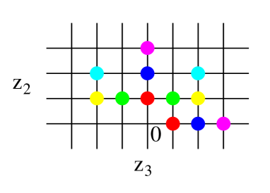
Figure 1: Pairs of values of $z_{3}$ at constant $z^{2}=-z_{3}^{2}-z_{2}^{2}$ used to evaluate the finite difference approximating the derivative with respect to $z\cdot P$ in (12). Each pair is distinguished by its color. The spacing of the grid is the lattice spacing $a$ (note that the displayed grid is not the underlying lattice itself, but it is a grid of relative distances on that lattice). The final result for $(L_{3}+2S_{3})/n$ is determined by the $z^{2}=-a^{2}$ case (red dots).

Obtaining the form (12) from (11), one integrates over the quark momenta $k_{T}$ and $k^{-}$. Formally, this implies the limits $z^{-}\rightarrow 0,z_{T}\rightarrow 0$ in (12), if one were to integrate over all momenta without any cutoff. However, the finite resolution implied by the lattice spacing $a$ implies a cutoff on momenta, or, formulated in $z$-space, quark operator separations smaller than $|z|=a$ cannot be resolved. Thus, the aforementioned limits $z^{-}\rightarrow 0,z_{T}\rightarrow 0$ will be understood to mean evaluation at fixed $-z^{2}=a^{2}$; likewise, the derivative with respect to $z_{3}$ (in the lattice frame) in (12) will be taken to mean a finite difference over the minimally resolved distance $a$. In the numerical calculations to be presented below, a range of $|z|$ was studied, with the case $|z|=a$ determining the final results. Fig. 1 shows pairs of values of $z_{3}$ at constant $z^{2}$ used to evaluate the finite difference approximating the derivative with respect to $z\cdot P$ in (12). Consistently, also the denominator $n$ in (12) is evaluated at the same $z^{2}$, matching the operators in numerator and denominator at finite lattice spacing.

Note that this (gauge-invariant) momentum cutoff scheme, with $z^{2}$ effectively defining the cutoff on momentum integrations, differs from the perturbative $\overline{\mbox{MS}}$ renormalization scheme. Conversion of the results to the latter would require a matching factor that has currently not yet been determined. Systematic deviations between the two schemes have, however, been estimated to be minor [24] when the momentum cutoff is comparable to the renormalization scale. The numerical results presented below corroborate that the systematic uncertainty associated with the connection to the $\overline{\mbox{MS}}$ scheme is not dominant compared to other uncertainties of the calculation.

In addition to the derivative with respect to $z\cdot P$, (12) calls for a derivative of the matrix element with respect to (transverse) momentum transfer. This derivative was realized using a direct derivative method [25, 26, 27] in order to avoid any systematic bias in its evaluation. The treatment is identical to that carried out in [27], and the reader is referred to the detailed description there for specifics.

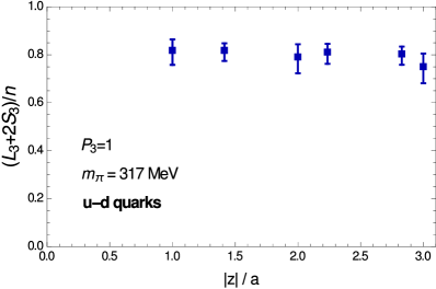
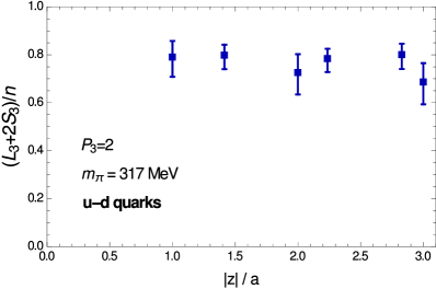
Figure 2: The combination $L_{3}+2S_{3}$, in units of the number of valence quarks $n$, obtained through the second Mellin moment of the twist-3 GPD $\widetilde{E}_{2T}$, as a function of the spatial cutoff $|z|$ used in evaluating (12), cf. discussion in main text. The two panels display two different proton momenta $P_{3}$ (values quoted in panel legends are given in units of $2\pi/\ell$, cf. main text).

Numerical data for the ratio (12) were obtained utilizing a 2+1-flavor clover fermion ensemble on a $32^{3}\times 96$ lattice with spacing $a=0.114\,\mbox{fm}=(1.73\,\mbox{GeV})^{-1}$. The pion mass on this ensemble is $m_{\pi}=317\,\mbox{MeV}$, and the source-sink separation employed to construct three-point functions was $10\,a=1.14\,\mbox{fm}$. Two proton momenta were explored, $P_{3}=2\pi/\ell,\,4\pi/\ell$, where $\ell=32\,a$ denotes the spatial lattice extent. Note that non-zero proton momentum is required to evaluate (13) (or spatial rotations thereof). The Ji definition of longitudinal orbital angular momentum (and likewise longitudinal spin) is boost-invariant, but lattice calculations at different $P_{3}$ may deviate from one another, e.g., as a result of discretization artefacts that will tend to increase with rising $P_{3}$. Fig. 2 displays results for $(L_{3}+2S_{3})/n$ for the two proton momenta, as a function of the spatial cutoff $|z|$ used in evaluating (12). The results are remarkably stable with respect to $|z|$ and agree within uncertainties for the two proton momenta, as expected. Of course, $L_{3}$ is expected to evolve nontrivially with the ultraviolet scale. However, at the given lattice spacing, there appears to be little ambiguity in the extraction of $(L_{3}+2S_{3})/n$, in view of its stability with respect to the implementation of the momentum cutoff.

To extract the final estimate for Ji longitudinal quark orbital angular momentum in the proton, the spin contribution $2S_{3}$ must be subtracted from (12). This contribution was previously evaluated on the same lattice ensemble in [28]. To achieve a combination of data that is as consistent as possible, the results from [28] were evaluated at matching fixed source-sink separation $10\,a$ (rather than using the extrapolation to the ground state also available there), yielding $2S_{3}=1.18(2)$. It should be noted that, whereas this result does not depend on renormalization scheme or scale (in the isovector case considered here), the handling of discretization effects in arriving at it does not fully coincide with the one implied by the momentum cutoff scheme adopted above in extracting $(L_{3}+2S_{3})/n$. However, being performed at a single lattice spacing, no quantitative assessment of the discretization error of the present calculation is possible in any case. In addition, the $|z|=a$ data from Fig. 2 were linearly extrapolated to $P_{3}=0$ for the purpose of combining the data. The final estimate of the isovector longitudinal Ji quark orbital angular momentum in the proton obtained in this manner is

$$L_{3}/n=-0.34(6)\ .$$ (17)

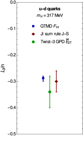
Figure 3: Isovector longitudinal Ji quark orbital angular momentum in the proton, in units of the number of valence quarks $n$, obtained in lattice calculations utilizing the three approaches given by eqs. (1), (2) and (3) discussed in the introduction.

5 Discussion

Fig. 3 places the result (17) into the context of alternative evaluations of isovector longitudinal Ji quark orbital angular momentum in the proton based on both the GTMD $F_{14}$, cf. (2), as well as Ji’s sum rule, cf. (1). The result employing the GTMD $F_{14}$ was obtained [27] on the same lattice ensemble as utilized in the present investigation, in the same quark momentum cutoff scheme as used in evaluating (12). The result employing Ji’s sum rule was obtained by interpolating data from [17] to the same pion mass as employed here; these data are given in the $\overline{\mbox{MS}}$ scheme at scale $\mu=2\,\mbox{GeV}$.

The various determinations agree within the statistical uncertainties; the different systematics inherent in the distinct approaches, including the schemes in which the ultraviolet divergences are handled, appear to only influence the results for the quark orbital angular momentum to an insignificant extent, compared to the statistical fluctuations. The magnitude of those fluctuations in the determination of quark orbital angular momentum via the twist-3 GPD $\widetilde{E}_{2T}$ is notable. It is much larger than the one using the GTMD $F_{14}$, obtained on the same ensemble with the same statistics (the Ji sum rule result cannot be directly compared in the same way concerning the statistical fluctuations, since it was obtained on different ensembles employing significantly smaller sets of samples). The main reason for the comparatively large statistical uncertainty of the result obtained using the twist-3 GPD $\widetilde{E}_{2T}$ is that it is realized through a difference of large numbers, $L_{3}=(L_{3}+2S_{3})-2S_{3}$, canceling a large part of the signal and thus enhancing the relative uncertainty. Also a less than optimal cancellation of fluctuations in the numerator and denominator of (12) may play a role, when the matrix element in the denominator (13) is rotated to align the $j$-direction with the direction of $P$ in (12), as remarked after eq. (13).

Nonetheless, the present study demonstrates the feasibility of extracting quark orbital angular momentum in the proton from the twist-3 GPD $\widetilde{E}_{2T}$, albeit requiring higher computational effort compared to other approaches to achieve comparable accuracy. Presumably also phenomenological studies employing the GPD $\widetilde{E}_{2T}$ would have to grapple with the numerical challenges inherent in the difference of large numbers required to determine the quark orbital angular momentum in the proton.

References

- [1] J. Ashman et al. [European Muon Collaboration], Phys. Lett. B206 (1988) 364.
- [2] J. Ashman et al. [European Muon Collaboration], Nucl. Phys. B328 (1989) 1.
- [3] X. Ji, Phys. Rev. Lett. 78 (1997) 610.
- [4] R. Jaffe and A. Manohar, Nucl. Phys. B337 (1990) 509.
- [5] Y. Hatta, Phys. Lett. B708 (2012) 186.
- [6] C. Lorcé and B. Pasquini, Phys. Rev. D 84 (2011) 014015.
- [7] S. Meißner, A. Metz and M. Schlegel, JHEP 0908 (2009) 056.
- [8] M. Burkardt, Phys. Rev. D 88, 014014 (2013).
- [9] X. Ji, X. Xiong and F. Yuan, Phys. Rev. Lett. 109, 152005 (2012).
- [10] A. Rajan, A. Courtoy, M. Engelhardt and S. Liuti, Phys. Rev. D 94, 034041 (2016).
- [11] C. Lorcé and B. Pasquini, Int. J. Mod. Phys. Conf. Ser. 20 (2012) 84.
- [12] A. Rajan, M. Engelhardt and S. Liuti, Phys. Rev. D 98, 074022 (2018).
- [13] M. Penttinen, M. Polyakov, A. Shuvaev and M. Strikman, Phys. Lett. B491 (2000) 96.
- [14] D. Kiptily and M. Polyakov, Eur. Phys. J. C 37 (2004) 105.
- [15] Y. Hatta and S. Yoshida, JHEP 10 (2012) 080.
- [16] P. Hägler et al. [LHP Collaboration], Phys. Rev. D 77, 094502 (2008).
- [17] J. D. Bratt et al. [LHP Collaboration], Phys. Rev. D 82, 094502 (2010).
- [18] M. Göckeler, R. Horsley, D. Pleiter, P. E. L. Rakow, A. Schäfer, G. Schierholz and W. Schroers [QCDSF Collaboration], Phys. Rev. Lett. 92, 042002 (2004).
- [19] G. Bali, S. Collins, M. Göckeler, R. Rödl, A. Schäfer and A. Sternbeck [RQCD Collaboration], Phys. Rev. D 100, 014507 (2019).
- [20] M. Deka, T. Doi, Y.-B. Yang, B. Chakraborty, S. J. Dong, T. Draper, M. Glatzmaier, M. Gong, H.-W. Lin, K.-F. Liu, D. Mankame, N. Mathur and T. Streuer, Phys. Rev. D 91 (2015), 014505 (2015).
- [21] C. Alexandrou, M. Constantinou, K. Hadjiyiannakou, K. Jansen, C. Kallidonis, G. Koutsou, A. Vaquero Avilés-Casco and C. Wiese, Phys. Rev. Lett. 119, 142002 (2017).
- [22] C. Alexandrou, S. Bacchio, M. Constantinou, J. Finkenrath, K. Hadjiyiannakou, K. Jansen, G. Koutsou, H. Panagopoulos and G. Spanoudes, Phys. Rev. D 101, 094513 (2020).
- [23] M. Engelhardt, Phys. Rev. D 95, 094505 (2017).
- [24] M. Ebert, J. Michel, I. Stewart and Z. Sun, JHEP 07 (2022) 129.
- [25] G. M. de Divitiis, R. Petronzio and N. Tantalo, Phys. Lett. B718, 589 (2012).
- [26] N. Hasan, J. R. Green, S. Meinel, M. Engelhardt, S. Krieg, J. Negele, A. Pochinsky and S. Syritsyn, Phys. Rev. D 97, 034504 (2018).
- [27] M. Engelhardt, J. R. Green, N. Hasan, S. Krieg, S. Meinel, J. Negele, A. Pochinsky and S. Syritsyn, Phys. Rev. D 102 (2020) 074505.
- [28] J. R. Green, N. Hasan, S. Meinel, M. Engelhardt, S. Krieg, J. Laeuchli, J. Negele, K. Orginos, A. Pochinsky and S. Syritsyn, Phys. Rev. D 95 (2017) 114502.