Optimal Control of General Impulsive VS-EIAR Epidemic Models with Application to Covid-19

Mamadou Abdoul DIOP1,3, Mohammed Elghandouri2,3,βˆ— and Khalil Ezzinbi2,3

1Department of Mathematics, Faculty of Applied Sciences and Technology, Gaston Berger University, Senegal.
2Cadi Ayyad University, Faculty of Sciences Semlalia, Departement of Mathematics, Marrakesh, Morocco.
3IRD, UMMISCO, F-93143, Bondy, Paris, France.


Abstract. In this work, we are interested in a VS-EIAR epidemiological model considering vaccinated individuals ${V_{i}:\hskip 2.84544pti=1,\ldots,n}$, where $n\in\mathbb{N}^{*}$. The dynamic of the VS-EIAR model involves several ordinary differential equations that describe the changes in the vaccinated, susceptible, infected, exposed, asymptomatic, and deceased population groups. Our aim is to reduce the number of susceptible, exposed, infected, and asymptomatic individuals by administering vaccination doses to susceptible individuals and treatment to infected population. To achieve this, we utilize optimal control theory to regulate the dynamic of our considered epidemic model within a terminal optimal time $\tau^{*}$. Pontryagin’s maximum principle (PMP) will be employed to establish the existence of an optimal control time $(v^{*}(t),u^{*}(t))$. We also incorporate an impulsive VS-EIAR epidemic model, with special attention given to immigration or the travel of certain population groups. Finally, we provide a numerical simulation to demonstrate the practical implementation of the theoretical findings.

Keywords. Optimal Control, Impulsive Epidemic Model, Mathematical Modeling, Ordinary Differential Equations, Covid-19.

††footnotetext: βˆ—Corresponding author. E-mail addresses: mamadou-abdoul.diop@ugb.edu.sn (M. A. Diop), medelghandouri@gmail.com (M. Elghandouri), ezzinbi@uca.ac.ma (K. Ezzinbi). Received xx xx, 20xx; Accepted xx xx, 20xx.

1. Introduction

Covid-19 presents itself as one of the most formidable global challenges, profoundly impacting economies, societies, and politics. The World Health Organization (WHO) officially reported the first case in Wuhan, China, on December 31, 2019 [1]. Notable respiratory symptoms such as cough, fever, breathing difficulties, and shortness of breath are prevalent indications of this infection. In severe cases, it can escalate into life-threatening conditions like pneumonia, severe acute respiratory syndrome, respiratory failure, and even death, as documented by the WHO reports. In the initial stages, quarantine and treatment were the primary measures employed to contain the spread of the disease. However, this approach came with substantial economic costs and further exacerbated existing crises, leading to prolonged recovery periods. Fortunately, we now have the advantage of vaccines, offering a more viable alternative to control the emergence of Covid-19, alleviating the need for strict quarantine measures. In this research, we delve into the application of this concept from a mathematical standpoint. Our study unveils a comprehensive mathematical model, surpassing existing literature, to address the dynamics of Covid-19. By offering a more in-depth and precise model, we aim to contribute to a deeper understanding of the pandemic’s spread and potential control strategies. Abbasi et al. [2] proposed an impulsive SQEIAR epidemic model to control the spread of Covid-19 using two control actions: quarantine for susceptible populations and treatment for those who are infected. Araz [4] developed a comprehensive mathematical model incorporating various scenarios of Covid-19 transmission, considering both susceptible and symptomatic infectious individuals. The study delves into stability analysis, the existence of optimal control strategies, and the positiveness of solutions. In [6], the authors proposed a nonlinear deterministic model to study the optimal controllability of Covid-19 using Pontryagin’s maximum principle (PMP). They established the existence of four time-dependent optimal control actions: $u_{1}^{*}$-implementing measures for social or physical distancing, $u_{2}^{*}$-cleaning contaminated surfaces using alcoholic products, $u_{3}^{*}$-advocating precautions for individuals exposed to the virus, whether symptomatic or not, and $u_{4}^{*}$-fumigating educational institutions of all levels, athletic complexes, business spaces, and places of worship. G. B. Libotte et al. [16] presented an SIR model aimed at identifying the most effective vaccination delivery control approach for the Covid-19 pandemic. The study proposes two optimal control strategies: the first focuses on reducing the number of infected individuals during treatments, while the second aims to simultaneously decrease both the number of affected population and the concentration of the recommended vaccine throughout the treatment process. Additionally, the authors addressed an inverse problem by employing Differential Evolution and Multi-objective Optimization Differential Evolution algorithms. These approaches were used to establish the existence of parameters for the compartmental SIR model. In [24], Shen and Chou proposed a novel optimal control model for Covid-19 to mitigate infection spread by implementing four control actions: prevention measures, vaccine control, rapid screening of individuals in the exposed group, and managing non-screened infected individuals. Various other strategies are explored in [7, 12, 13, 18, 19, 20, 21, 25, 26] and the references cited within these works.

In [2], the authors focus on minimizing the number of susceptible, exposed, infected, and asymptomatic individuals, while increasing the number of quarantined and recovered individuals using optimal control theory. They achieve this by minimizing a functional cost $\mathcal{J}$ related to treatment $U(t)\in[0,1]$ and quarantine $\lambda(t)\in\left[0,1\right]$ within an optimal time interval. The study utilizes Pontryagin’s maximum principle (PMP) to establish the existence of an optimal control time $(U^{*}(t),\lambda^{*}(t),T^{*})$ at which the cost functional $\mathcal{J}$ reaches its minimum [2, Sections 2 and 4]. However, considering the high costs associated with quarantine, particularly when multiple vaccines against Covid-19 are available, our research proposes an alternative approach. We present an optimal control VS-EIAR epidemic model that employs vaccination instead of quarantine. The key idea is to administer a number $n$ of vaccine doses to susceptible individuals, assuming that the recovered population is immune to reinfection for a certain period or against the same virus variant. Additionally, we assume that individuals vaccinated with the maximum doses are less susceptible to infection, resulting in a negligible or null infection rate ($\delta_{n}\simeq 0$) for this subgroup. It is also reasonable to assume that the number of individuals vaccinated by the $i^{th}$ dose is always greater than the number of individuals vaccinated by the $(i+1)^{th}$ dose. Further details can be found in Section 2, along with Fig 1 for visualization.

In the context of the impulsive case, the model takes into account immigration or travel of certain populations. Impulsive epidemiological models have a significant biological impact on epidemic modeling, as impulses are added to enhance the accessibility and applicability of biological studies. The literature on this subject is richer, and it is beyond the scope of this discussion to enumerate all the relevant issues. Interested readers can refer to works such as [8, 9, 10, 11, 14, 15, 23, 27] and the references therein for further exploration. In particular, Agarwal et al. [11] discussed the controllability of a generalized time-varying delay SEIR epidemic model using impulsive vaccination controls. The authors suggest that the differences between the SEIR model and its appropriate reference model can be reduced through impulsive vaccination. Hui and Chen in [14] considered the impulsive vaccination strategies to study the global stability of some epidemic SIR models. They proved that impulsive vaccination strategies are more applicable with a best effect than classical vaccination strategies. Wang et al. [27] studied the dynamics of an impulsive epidemiological model for pest control. The authors proved that susceptible pest eradication solutions are globally stable if the impulsive time is smaller than some specific critical values. In this work, we included an impulse population from the community to explain how Covid-19 spreads over time more through immigration and individual travel. More details can be found in Section 4, see also Fig 2.

In summary, this work is organized as follows. In Section 2, we provide a detailed explanation of the considered VS-EIAR epidemic model and present the mathematical model describing its dynamic. Section 3 elaborates on the optimal control strategy applied to our proposed VS-EIAR epidemic model. In Section 4, we delve into the details of the proposed impulsive VS-EIAR dynamic model. The existence of the optimal control within an optimal time interval, using Pontryagin’s maximum principle, is demonstrated in Section 5. An application to Covid-19 is presented in Section 6. Furthermore, in Section 7, we conduct a comparison between three different diseases (Covid-19, Ebola, and Influenza). Section 8 offers a conclusion. The last one in an appendix.

2. VS-EIAR Epidemic Model

In this section, we present the VS-EIAR epidemic model, aimed at controlling disease propagation within a short time-frame. To achieve this goal, we exclude natural mortality and births from the model. The nonlinear VS-EIAR epidemiological model consists of $n+6$ non-negative state variables: $V_{1}(t)$, $\ldots$ , $V_{n}(t)$, $S(t)$, $E(t)$, $A(t)$, $I(t)$, $R(t)$, and $D(t)$. Here, $V_{i}(t)$, with $i=1,\ldots,n$, represents the total number of individuals who have received $i$ dose(s) of the vaccine at time $t$ but have not yet received the $(i+1)^{th}$ dose for $i=1,\ldots,n-1$. $S(t)$ denotes the total number of individuals at risk of contracting the infection at time $t$; they are susceptible but not infected yet. Upon infection, susceptible individuals join the exposed population group, $E(t)$, representing the total number of infected individuals who cannot transmit the infection at time $t$. It is important to note that some of the exposed individuals can eventually become infectious and transmit the disease at the rate $k$, while others may exhibit asymptomatic symptoms. We denote the total number of infected individuals without visible symptoms at time $t$ as $A(t)$, and those with visible symptoms as $I(t)$. The fraction $z$ of exposed individuals join the group of infected population and can transmits the disease to others when the rest of them moves to the group of population who are infected but didn’t have any visible symptoms. Finally, a fraction $p$ of asymptomatic population moves to the group of population who are recovered from the pandemic at time $t$ that we denote by $R(t)$, when the fraction $(1-p)$ moves to the group of infected population. A part $(1-\alpha)$ of infected population will die because of the infection, when the rest of them will be considered as recovered population. According to the advice from the World Health Organization (WHO) and viral disease specialists, vaccination should not be administered to those currently infected or recently recovered from the virus, at least for a specified period of time. Consequently, our control vaccination strategy targets susceptible individuals. Figure 1 summarizes the biological dynamic of our considered model. It is natural to assume that a susceptible individual cannot take the $(i+1)^{th}$ dose just if it has the $i^{th}$ dose, which explains the fact that

$\gamma_{1}\geq\gamma_{2}\geq\cdots\geq\gamma_{n}\geq 0$.  ($\gamma_{1}>0$).

On the other hand, we assume that individuals who have received the most doses are less likely to get the infection than the population who have received fewer doses, which explains the fact that

$\delta_{1}\geq\delta_{2}\geq\cdots\geq\delta_{n-1}\geq\delta_{n}\simeq 0$.

We assume that $\gamma_{i}\geq\delta_{i}$ for $i=1,2,\ldots,n$, where $\beta,\eta,p,k,z,\alpha,f\in[0,1]$. The main idea is to use optimal control theory to eradicate the spread of the epidemic by applying vaccination $v(t)$ to susceptible population and treatment $u(t)$ to infected population. The dynamic of our control model is described by the following ODE:

$$\left\{\begin{array}[]{l}\dot{V}_{1}(t)=\gamma_{1}v(t)S(t)-\gamma_{2}v(t)V_{1}(t)-\delta_{1}V_{1}(t)\\ \\ \left\{\begin{array}[]{l}\dot{V}_{i}(t)=\gamma_{i}v(t)V_{i-1}(t)-\gamma_{i+1}v(t)V_{i}(t)-\delta_{i}V_{i}(t),\\ \\ \text{for}\hskip 2.84544pti=2,3,\ldots,n-1,\end{array}\right.\\ \\ \dot{V}_{n}(t)=\gamma_{n}v(t)V_{n-1}(t)\\ \\ \dot{S}(t)=-(\beta\Lambda(t)+\gamma_{1}v(t))S(t)\\ \\ \dot{E}(t)=\beta\Lambda(t)S(t)-kE(t)+\sum\limits_{i=1}^{n-1}\delta_{i}V_{i}(t)\\ \\ \dot{A}(t)=(1-z)kE(t)-\eta A(t)\\ \\ \dot{I}(t)=zkE(t)+(1-p)\eta A(t)-fI(t)-u(t)I(t)\\ \\ \dot{R}(t)=\alpha fI(t)+u(t)I(t)+p\eta A(t)\\ \\ \dot{D}(t)=(1-\alpha)fI(t),\end{array}\right.$$ (2.1)

for $t\in[0,\tau]$, $\tau\in\mathbb{R}^{+}$, where $\Lambda(t)=\varepsilon E(t)+(1-q)I(t)+\mu A(t)$. Here, $\varepsilon>0$, $1-q>0$, and $\mu>0$ are the reduced transmissibility factors from exposed, infected, and asymptomatic contacts, respectively. The initial condition is given by $(S(0)$, $E(0)$, $A(0)$, $I(0)$, $R(0)$, $D(0)$, $V_{1}(0)$,$\ldots$, $V_{n}(0))$ $=(S_{0}$, $E_{0}$ ,$A_{0}$, $I_{0}$, $R_{0}$, $D_{0}$, $V_{1,0}$,$\ldots$,$V_{n,0})$. Let $N(t)=S(t)+E(t)+A(t)+I(t)+R(t)+\sum\limits_{i=1}^{n}V_{i}(t)$ be the total population at time $t$. We define the admissible controls sets $U^{1}_{ad}$ and $U_{ad}^{2}$ as follows

$U^{1}_{ad}=\left\{v\mid v\text{ is almost everywhere continuous from }\mathbb{R}^{+}\text{ to }\left[0,\frac{1}{\gamma_{1}}\right]\right\}$,

and

$U^{2}_{ad}=\left\{u\mid u\text{ is almost everywhere continuous from }\mathbb{R}^{+}\text{ to }\left[0,1\right]\right\}$.

2.1. Existence of solutions

The following theorem ensures the existence and uniqueness of the solutions for equation (2.1).

Theorem 2.1.

Let $V_{1,0}\geq 0$, $\ldots$, $V_{n,0}\geq 0$, $S_{0}\geq 0$, $E_{0}\geq 0$, $A_{0}\geq 0$, $I_{0}\geq 0$, $R_{0}\geq 0$, and $D_{0}\geq 0$. Let $v\in U^{1}_{ad}$ and $u\in U^{2}_{ad}$ be fixed. Then, equation (​2.1​)italic-(2.1italic-)\eqref{eq 1} has a unique positive bounded solution defined on $\mathbb{R}^{+}$.

Proof.

See the Appendix. ∎

Remark 2.1.

Why do we need to consider controls? The basic reproduction number of our model without controls (The SEIAR epidemic model) is given by the following expression:

$$\mathcal{R}_{0}=\beta N_{0}\left[\frac{z}{\alpha f}+\frac{\mu(1-z)}{\eta}\right].$$ (2.2)

If $\mathcal{R}_{0}<1$, the infection dies out. However, if $\mathcal{R}_{0}>1$, an epidemic occurs, and it becomes imperative to implement controls. In the case of the Covid-19 example discussed in Section 6, we have $\mathcal{R}_{0}=1.52>1$ with $\beta=5\times 10^{-4}$. Consequently, the Covid-19 epidemic exists, necessitating the implementation of controls. In general, as the transmission coefficient $\beta$ increases or the recovery rate from the infectious class decreases, the basic reproduction number of our model increases, indicating the potential for an epidemic, and thus emphasizing the importance of implementing controls.

3. Optimal Control Problem of the VS-EIAR Epidemic Model

In this section, we present a strategy based on optimal control theory to minimize the number of susceptible, exposed, infected, and asymptomatic individuals by implementing vaccination $v(t)$ for susceptible individuals and treatment $u(t)$ for infected individuals. Therefore, the main objective is to minimize the cost functional $\mathcal{J}$ defined on $U^{1}_{ad}\times U^{2}_{ad}\times\mathbb{R}^{*}_{+}$ by

π’₯​(v,u,Ο„)=∫0Ο„[𝒦​(S​(s),E​(s),A​(s),I​(s))+Οƒ02​u​(s)2+βˆ‘i=1nΟƒi​γi22​v​(s)2]​𝑑s+ℳ​(Ο„),π’₯π‘£π‘’πœsuperscriptsubscript0𝜏delimited-[]𝒦𝑆𝑠𝐸𝑠𝐴𝑠𝐼𝑠subscript𝜎02𝑒superscript𝑠2superscriptsubscript𝑖1𝑛subscriptπœŽπ‘–superscriptsubscript𝛾𝑖22𝑣superscript𝑠2differential-dπ‘ β„³πœ\begin{array}[]{l}\mathcal{J}(v,u,\tau)=\displaystyle\int_{0}^{\tau}\left[\mathcal{K}\left(S(s),E(s),A(s),I(s)\right)+\dfrac{\sigma_{0}}{2}u(s)^{2}+\sum\limits_{i=1}^{n}\dfrac{\sigma_{i}\gamma_{i}^{2}}{2}v(s)^{2}\right]ds+\mathcal{M}(\tau),\end{array} (3.1)

where

$\mathcal{K}\left(S(t),E(t),A(t),I(t)\right)=\omega_{1}S(t)+\omega_{2}E(t)+\omega_{3}A(t)+\omega_{4}I(t)$ for $t\in[0,\tau]$,

and $\mathcal{M}(\cdot)$ is a convex non-negative increasing continuous function such that $\lim\limits_{t\to+\infty}\mathcal{M}(t)=+\infty$. The term $\mathcal{K}\left(S(t),E(t),A(t),I(t)\right)$ represents the epidemic cost at time $t$. It is a combination of weighted contributions from susceptible $(S)$, exposed $(E)$, asymptomatic $(A)$, and infected $(I)$ individuals. Each of these groups has an associated weight $\omega_{i}$ $(i=1,2,3,4)$, which can be interpreted as the relative importance or severity of the epidemic state. This term evaluates the general effects of the epidemic on the population at any given time. The term $(\sigma_{0}/2)u(t)^{2}$ represents the control cost associated with the treatment measurement. The control $u(t)$ is utilised to administer the treatment intervention amidst the epidemic. The parameter $\sigma_{0}$ represents the treatment controller’s gain, which is used to achieve a balance between the importance of implementing the treatment and its related expenses. The term $\sum\limits_{i=1}^{n}(\sigma_{i}\gamma_{i}^{2}/2)v(t)^{2}$ represents the control cost associated with the vaccinated individuals. The control $v(t)$ is used to manage the vaccination strategy for $n$ different groups of vaccinated individuals $V_{i}$ $(i=1,\ldots,n)$. The parameter $\sigma_{i}$ represents the gain of each vaccination controller, where $\gamma_{i}$ represents the effectiveness of the vaccination for each group $V_{i}$. This term quantifies the cost of implementing vaccination measures in the control of the epidemic. The term $\mathcal{M}(\tau)$ represents a terminal cost associated with the epidemic control problem. It is a function of the final time $\tau$ and likely incorporates additional costs or penalties related to the final state of the epidemic. The condition $\lim\limits_{t\to+\infty}\mathcal{M}(t)=+\infty$ reflects the realistic scenario that the costs associated with disease control will increase over time.

The aim would be to find an optimal control $(v^{*},u^{*})$ in an optimal finite time $\tau^{*}$ such that

$\mathcal{J}(v^{*},u^{*},\tau^{*})=\min\left\{\mathcal{J}(v,u,\tau)\mid(v,u)\in U_{ad}^{1}\times U_{ad}^{2},\hskip 2.84544pt\tau\in\mathbb{R}^{+}_{*}\right\}$.

Theorem 3.1.

There exists a unique $(v^{*},u^{*},\tau^{*})\in U^{1}_{ad}\times U^{2}_{ad}\times\mathbb{R}^{+}_{*}$ at which $\mathcal{J}$ attains its minimum.

Proof.

Let $\mathcal{I}=\min\left\{\mathcal{J}(v,u,\tau)\mid(v,u)\in U_{ad}^{1}\times U_{ad}^{2},\hskip 2.84544pt\tau\in\mathbb{R}^{+}_{*}\right\}$. Since $0\leq\mathcal{I}<+\infty$, it follows that there exists a sequence $((v_{m},u_{m},\tau_{m}))_{m\geq 1}\subseteq U^{1}_{ad}\times U^{2}_{ad}\times\mathbb{R}^{+}_{*}$ such that $\lim\limits_{m\to+\infty}\mathcal{J}(v_{m},u_{m},\tau_{m})=\mathcal{I}$. The sequence $(\tau_{m})_{m\geq 1}$ is bounded in $\mathbb{R}^{+}_{*}$. Indeed, assume that $\tau_{m}\to+\infty$ as $m\to+\infty$, then we have $\lim\limits_{m\to+\infty}\mathcal{J}(v_{m},u_{m},\tau_{m})=+\infty$ (because of the positiveness of sates and $\lim\limits_{m\to+\infty}\mathcal{M}(\tau_{m})=+\infty$). That is a contradiction, since $\lim\limits_{m\to+\infty}\mathcal{J}(v_{m},u_{m},\tau_{m})=\mathcal{I}<+\infty$, which means that $(\tau_{m})_{m\geq 1}$ is bounded in $\mathbb{R}^{+}_{*}$. Let $\bar{\tau}>0$ such that $0\leq\tau_{m}\leq\bar{\tau}$ for $m\geq 1$. Hence, there exists a sub-sequence of $(\tau_{m})_{m\geq 1}$ that we continue to denote by the same index $m\geq 1$ such that $\tau_{m}\to\tau^{*}$ as $m\to+\infty$ for some $\tau^{*}\in\mathbb{R}^{+}_{*}$. Let $t\in[0,\tau_{m}[$, since $0\leq v_{m}(t)\leq\dfrac{1}{\gamma_{1}}$, it follows that there exists a sub-sequence of $(v_{m}(t))_{m\geq 1}$ that we continue to denote by the same index $m\geq 1$ such that $v_{m}(t)\to v^{*}(t)$ as $m\to+\infty$. If $t=\tau_{m}$, using the fact that $0\leq v_{m}(\tau_{m})\leq\dfrac{1}{\gamma_{1}}$, similarly, we can affirm that there exists a sub-sequence of $(v_{m}(\tau_{m}))_{m\geq 1}$ that we continue to denote by the same index $m\geq 1$ such that $v_{m}(\tau_{m})\to w^{*}\in\left[0,\frac{1}{\gamma_{1}}\right]$ as $m\to+\infty$. Let $v^{*}(\tau^{*})=w^{*}$. We can see that $v^{*}\in U^{1}_{ad}$. In the next, we show that $\lim\limits_{m\to+\infty}\displaystyle\int_{0}^{\tau_{m}}v_{m}(s)^{2}ds=\displaystyle\int_{0}^{\tau^{*}}v^{*}(s)^{2}ds$. Since Ο‡[0,Ο„m]​(s)​vm​(s)β†’Ο‡[0,Ο„βˆ—]​(s)​vβˆ—β€‹(s)β†’subscriptπœ’0subscriptπœπ‘šπ‘ subscriptπ‘£π‘šπ‘ subscriptπœ’0superscriptπœπ‘ superscript𝑣𝑠\chi_{[0,\tau_{m}]}(s)v_{m}(s)\to\chi_{[0,\tau^{*}]}(s)v^{*}(s) as $m\to+\infty$ for a.e $s\in\mathbb{R}^{+}$, and Ο‡[0,Ο„m]​(s)​vm​(s)≀1Ξ³1​χ[0,τ¯]​(s)subscriptπœ’0subscriptπœπ‘šπ‘ subscriptπ‘£π‘šπ‘ 1subscript𝛾1subscriptπœ’0Β―πœπ‘ \chi_{[0,\tau_{m}]}(s)v_{m}(s)\leq\dfrac{1}{\gamma_{1}}\chi_{[0,\bar{\tau}]}(s) for a.e $s\in\mathbb{R}^{+}$, ($\chi_{J}$ is the characteristic function on an interval $J\subseteq\mathbb{R}^{+}$), by the dominated convergence theorem, we obtain that

limmβ†’+∞∫0Ο„mvm​(s)2​𝑑s=limmβ†’+∞∫0+βˆžΟ‡[0,Ο„m]​(s)​vm​(s)2​𝑑s=∫0+βˆžΟ‡[0,Ο„βˆ—]​(s)​vβˆ—β€‹(s)2​𝑑s=∫0Ο„βˆ—vβˆ—β€‹(s)2​𝑑s.subscriptβ†’π‘šsuperscriptsubscript0subscriptπœπ‘šsubscriptπ‘£π‘šsuperscript𝑠2differential-d𝑠subscriptβ†’π‘šsuperscriptsubscript0subscriptπœ’0subscriptπœπ‘šπ‘ subscriptπ‘£π‘šsuperscript𝑠2differential-d𝑠superscriptsubscript0subscriptπœ’0superscriptπœπ‘ superscript𝑣superscript𝑠2differential-d𝑠superscriptsubscript0superscript𝜏superscript𝑣superscript𝑠2differential-d𝑠\lim\limits_{m\to+\infty}\displaystyle\int_{0}^{\tau_{m}}v_{m}(s)^{2}ds=\lim\limits_{m\to+\infty}\displaystyle\int_{0}^{+\infty}\chi_{[0,\tau_{m}]}(s)v_{m}(s)^{2}ds=\displaystyle\int_{0}^{+\infty}\chi_{[0,\tau^{*}]}(s)v^{*}(s)^{2}ds=\displaystyle\int_{0}^{\tau^{*}}v^{*}(s)^{2}ds.

Similarly, we can prove that there exists $u^{*}\in U^{2}_{ad}$, such that $\lim\limits_{m\to+\infty}\displaystyle\int_{0}^{\tau_{m}}u_{m}(s)^{2}ds=\displaystyle\int_{0}^{\tau^{*}}u^{*}(s)^{2}ds$.

Let $x_{m}(t)=\left(S_{m}(t),E_{m}(t),A_{m}(t),I_{m}(t),R_{m}(t),D_{m}(t),V_{m,1}(t),\ldots,V_{m,n}(t)\right)^{T}$ be the state value of equation (2.1) at time $t$ corresponding to the control function $w_{m}(t)=(v_{m}(t),u_{m}(t))$. Taking in account these notations, equation (2.1) can be written as follows:

$$\left\{\begin{array}[]{l}\dot{x}_{m}(t)=F(x_{m}(t),w_{m}(t)),\quad t\in[0,\tau_{m}],\\ x_{m}(0)=x_{0},\end{array}\right.$$

where $F$ is a well defined function (see the Appendix). Hence,

xm​(t)=x0+∫0tF​(xm​(s),wm​(s))​𝑑s​ for ​t∈[0,Ο„m].subscriptπ‘₯π‘šπ‘‘subscriptπ‘₯0superscriptsubscript0𝑑𝐹subscriptπ‘₯π‘šπ‘ subscriptπ‘€π‘šπ‘ differential-d𝑠 for 𝑑0subscriptπœπ‘šx_{m}(t)=x_{0}+\displaystyle\int_{0}^{t}F(x_{m}(s),w_{m}(s))ds\hskip 2.84544pt\text{ for }\hskip 2.84544ptt\in[0,\tau_{m}]. (3.2)

Since $N(t)\leq N_{0}$ for $t\in[0,\tau_{m}]$ (see Proof of Theorem 2.1 in the Appendix), it follows that

$\|x_{m}(t)\|\leq(n+6)N(t)\leq(n+6)N_{0}$ for $t\in[0,\tau_{m}]$,

which means that $(x_{m}(t))_{m\geq 1}$ is bounded in $\mathbb{R}_{+}^{n+6}$. If $t\in[0,\tau_{m}[$, then there exists a sub-sequence of $(x_{m}(t))_{m\geq 1}$ that we continue to denote by the same index $m\geq 1$ such that $(x_{m}(t))_{m\geq 1}$ converges to some $z^{*}(t)\in\mathbb{R}_{+}^{n+6}$ as $m\to+\infty$. If $t=\tau_{m}$, similarly, we can prove that there exists a sub-sequence of $(x_{m}(\tau_{m}))_{m\geq 1}$ that we continue to denote by the same index $m\geq 1$ such that $(x_{m}(\tau_{m}))_{m\geq 1}$ converges to some $\bar{x}^{*}\in\mathbb{R}_{+}^{n+6}$. Let $z^{*}(\tau^{*})=\bar{x}^{*}$. It follow from (3.2) that

$z^{*}(t)=z^{*}(0)+\displaystyle\int_{0}^{t}F(z^{*}(s),w^{*}(s))ds\text{ for }t\in[0,\tau^{*}]$,

where $w^{*}(\cdot)=(v^{*}(\cdot),u^{*}(\cdot))$. That is $z^{*}(t)=x^{*}(t)$ the state value of equation (2.1) corresponding to the control functions $(v^{*}(t),u^{*}(t))$ at time $t\in[0,\tau^{*}]$. As a remark, we can show that Ο‡[0,Ο„m]​(s)​𝒦​(Sm​(s),Em​(s),Am​(s),Im​(s))subscriptπœ’0subscriptπœπ‘šπ‘ π’¦subscriptπ‘†π‘šπ‘ subscriptπΈπ‘šπ‘ subscriptπ΄π‘šπ‘ subscriptπΌπ‘šπ‘ \chi_{[0,\tau_{m}]}(s)\mathcal{K}\left(S_{m}(s),E_{m}(s),A_{m}(s),I_{m}(s)\right) converges to Ο‡[0,Ο„βˆ—]​(s)​𝒦​(Sβˆ—β€‹(s),Eβˆ—β€‹(s),Aβˆ—β€‹(s),Iβˆ—β€‹(s))subscriptπœ’0superscriptπœπ‘ π’¦superscript𝑆𝑠superscript𝐸𝑠superscript𝐴𝑠superscript𝐼𝑠\chi_{[0,\tau^{*}]}(s)\mathcal{K}\left(S^{*}(s),E^{*}(s),A^{*}(s),I^{*}(s)\right) for a.e $s\in\mathbb{R}^{+}$ as $m\to+\infty$, where $S^{*}(\cdot)$, $E^{*}(\cdot)$, $A^{*}(\cdot)$, and $I^{*}(\cdot)$ are the state values of the susceptible, exposed, asymptomatic, and infected populations, respectively, corresponding to the control functions $(v^{*}(\cdot),u^{*}(\cdot))$. Because of the continuity of $\mathcal{M}(\cdot)$, we deduce that $\lim\limits_{m\to+\infty}\mathcal{M}(\tau_{m})=\mathcal{M}(\tau^{*})$. Using the fact that $\mathcal{J}(\cdot,\cdot,\cdot)$ is convex, we conclude that

$\mathcal{I}\leq\mathcal{J}(v^{*},u^{*},\tau^{*})\leq\liminf\limits_{m\to+\infty}\mathcal{J}(v_{m},u_{m},\tau_{m})=\lim\limits_{m\to+\infty}\mathcal{J}(v_{m},u_{m},\tau_{m})=\mathcal{I}$.

As a consequence, $\mathcal{I}=\mathcal{J}(v^{*},u^{*},\tau^{*})$. For the uniqueness, see Theorem 3.2. ∎

Let $X(t)=\left(S(t),E(t),A(t),I(t),R(t),D(t),V_{1}(t),\ldots,V_{n}(t)\right)^{T}$. Define the Hamiltonian function $H$ by

$H(X(t),u(t),v(t),P(t),Q(t),t)=G(t)+[P(t),Q(t)]^{T}\dot{X}(t)$,

for

$G(t)=\mathcal{K}\left(S(t),E(t),A(t),I(t)\right)+\dfrac{\sigma_{0}}{2}u(t)^{2}+\left(\sum\limits_{i=1}^{n}\dfrac{\sigma_{i}\gamma_{i}^{2}}{2}\right)v(t)^{2}$,

$P(t)=[p_{1}(t),p_{2}(t),\ldots,p_{5}(t)]$ and $Q(t)=[q_{1}(t),q_{2}(t),\ldots,q_{n}(t)]$.

Then,

$\displaystyle H$ $\displaystyle=$ $\displaystyle\omega_{1}S(t)+\omega_{2}E(t)+\omega_{3}A(t)+\omega_{4}I(t)+\dfrac{\sigma_{0}}{2}u(t)^{2}+\left(\sum\limits_{i=1}^{n}\dfrac{\sigma_{i}\gamma_{i}^{2}}{2}\right)v(t)^{2}$
$\displaystyle+p_{1}(t)\dot{S}(t)+p_{2}(t)\dot{E}(t)+p_{3}(t)\dot{A}(t)+p_{4}(t)\dot{I}(t)+p_{5}(t)\dot{R}(t)+p_{6}(t)\dot{D}(t)$
$\displaystyle+\sum\limits_{i=1}^{n}q_{i}(t)\dot{V}_{i}(t).$

Moreover,

$\displaystyle\dot{P}(t)=-\left[\frac{\partial H}{\partial S(t)},\frac{\partial H}{\partial E(t)},\frac{\partial H}{\partial A(t)},\frac{\partial H}{\partial I(t)},\frac{\partial H}{\partial R(t)},\dfrac{\partial H}{\partial D(t)}\right],$ (3.3)

and

$\displaystyle\dot{Q}(t)=-\left[\frac{\partial H}{\partial V_{1}(t)},\ldots,\frac{\partial H}{\partial V_{n}(t)}\right].$ (3.4)

The following Theorem is the main result in this section. It provides the explicit forms of $u^{*}$ and $v^{*}$.

Theorem 3.2.

Let $(v^{*},u^{*})$ be the optimal controls of equation (​2.1​)italic-(2.1italic-)\eqref{eq 1} and $S^{*}$, $E^{*}$, $A^{*}$, $I^{*}$, $R^{*}$,$D^{*}$, $V_{1}^{*}$,$\ldots$,$V_{n}^{*}$ are the corresponding states values. Then,

$$u^{*}(t)=\max\left\{\min\left\{\dfrac{I^{*}(t)\left[p_{4}(t)-p_{5}(t)\right]}{\sigma_{0}},1\right\},0\right\},$$

and

$$v^{*}(t)=\max\left\{\min\left\{\dfrac{W(t)}{\left(\sum\limits_{i=1}^{n}\sigma_{i}\gamma_{i}^{2}\right)},\dfrac{1}{\gamma_{1}}\right\},0\right\},$$

where

$$W(t)=\gamma_{1}S^{*}(t)[p_{1}(t)-q_{1}(t)]+\gamma_{2}q_{1}(t)V_{1}^{*}(t)+\sum\limits_{i=2}^{n-1}q_{i}(t)[\gamma_{i+1}V_{i}^{*}(t)-\gamma_{i}V^{*}_{i-1}(t)],$$ (3.5)

and $p_{1}$, $p_{2}$, $p_{3}$, $p_{4}$, $p_{5}$, $p_{6}$, $q_{1}$, $\ldots$, $q_{n}$ are the solutions of the following adjoint equation:

$$\left\{\begin{array}[]{l}\dot{p}_{1}(t)=\beta\Lambda^{*}(t)\left[p_{1}(t)-p_{2}(t)\right]+\gamma_{1}v^{*}(t)\left[p_{1}(t)-q_{1}(t)\right]-\omega_{1}\\ \\ \dot{p}_{2}(t)=\beta\varepsilon S^{*}(t)p_{1}(t)+\left(k-\beta\varepsilon S^{*}(t)\right)p_{2}(t)-(1-z)kp_{3}(t)-zkp_{4}(t)-\omega_{2}\\ \\ \dot{p}_{3}(t)=\beta\mu S^{*}(t)\left[p_{1}(t)-p_{2}(t)\right]+\eta p_{3}(t)-(1-p)\eta p_{4}(t)-\omega_{3}\\ \\ \dot{p}_{4}(t)=\beta(1-q)S^{*}(t)\left[p_{1}(t)-p_{2}(t)\right]+u^{*}(t)\left[p_{4}(t)-p_{5}(t)\right]+f(p_{4}(t)\\ \\ \hskip 36.98866pt-\alpha p_{5}(t))-\hskip 2.84544pt(1-\alpha)fp_{6}(t)-\omega_{4}\\ \\ \dot{p}_{5}(t)=0\\ \\ \dot{p}_{6}(t)=0\\ \\ \dot{q}_{1}(t)=\delta_{1}\left[q_{1}(t)-p_{2}(t)\right]+\gamma_{2}v^{*}(t)\left[q_{1}(t)-q_{2}(t)\right]\\ \\ \dot{q}_{i}(t)=-\delta_{i}p_{2}(t)+(\gamma_{i+1}v^{*}(t)+\delta_{i})q_{i}(t)\quad(\text{for }i=2,3,\ldots,n-1)\\ \\ \dot{q}_{n}(t)=0,\end{array}\right.$$

for $t\in[0,\tau^{*}]$ in which $p_{j}(\tau^{*})=q_{i}(\tau^{*})=0$ for $j=1,\ldots,6$ and $i=1,\ldots,n$. Here, $\Lambda^{*}(t)=\varepsilon E^{*}(t)+(1-q)I^{*}(t)+\mu A^{*}(t)$ for $t\in[0,\tau^{*}]$.

Proof.

See the Appendix. ∎

Remark 3.1.

The control objectives are to reduce the number of groups $S$, $E$, $A$, and $I$ in an optimal finite time $\tau^{*}$ by applying vaccination and treatment strategies for susceptible and infected individuals. The variation of susceptible population takes the following form:

$\dot{S}(t)=-\Theta(t)S(t)$ for $t\geq 0$,

where $\Theta(t)=\beta\Lambda(t)+\gamma_{1}v(t)>0$ for $t\geq 0$ (because of the positiveness of sates and parameters, moreover, $v(t)$ is the control input and when needed, we can take $0<v(t)<\frac{1}{\gamma_{1}}$), that is the changes of $S(t)$ are subtractive over time, moreover,

S​(t)=exp⁑(βˆ’βˆ«0tΞ˜β€‹(s)​𝑑s)​S​(0)𝑆𝑑superscriptsubscript0π‘‘Ξ˜π‘ differential-d𝑠𝑆0S(t)=\exp\left(-\displaystyle\int_{0}^{t}\Theta(s)ds\right)S(0) for $t\geq 0$.

Since $S(0)>0$, it follows that $S(t)\to 0$ asymptotically as $t\to+\infty$. According to equation (2.1), the variation of $V_{1}(t)$ for $t\geq 0$ can be written as follows:

$\dot{V}_{1}(t)=-\Theta_{1}(t)V_{1}(t)+\gamma_{1}v(t)S(t)$ for $t\geq 0$,

where $\Theta_{1}(t)=\delta_{1}+\gamma_{2}v(t)>0$ for $t\geq 0$. Therefore,

$\displaystyle V_{1}(t)$ $\displaystyle=$ $\displaystyle R_{1}(t,0)V_{1}(0)+\gamma_{1}\displaystyle\int_{0}^{t}R_{1}(t,s)v(s)S(s)ds$
$\displaystyle=$ $\displaystyle R_{1}(t,0)V_{1}(0)+\gamma_{1}\displaystyle\int_{0}^{t}R_{1}(t,t-s)v(t-s)S(t-s)ds$
$\displaystyle=$ $\displaystyle R_{1}(t,0)V_{1}(0)+\gamma_{1}\displaystyle\int_{0}^{+\infty}\chi_{[0,t]}(s)R_{1}(t,t-s)v(t-s)S(t-s)ds,$

where $R_{1}(t,s)=\exp\left(-\int_{s}^{t}\Theta_{1}(r)dr\right)$ for $t\geq s\geq 0$. Since $V_{1}(0)>0$, $R_{1}(t,0)\to 0$, $\chi_{[0,t]}(s)R_{1}(t,t-s)v(t-s)S(t-s)\to 0$ as $t\to+\infty$ (because $v(\cdot)$ and $R_{1}(\cdot,\cdot)$ are bounded and $S(t)\to 0$ as $t\to+\infty$), and $R_{1}(t,t-s)v(t-s)S(t-s)\leq\frac{S(0)e^{-\delta_{1}s}}{\gamma_{1}}$, we use dominated convergence theorem, we obtain that $V_{1}(t)\to 0$ as $t\to+\infty$. In a similar manner, we get that

$\displaystyle V_{i}(t)$ $\displaystyle=$ $\displaystyle R_{i}(t,0)V_{i}(0)+\gamma_{i}\displaystyle\int_{0}^{t}R_{i}(t,s)v(s)V_{i-1}(s)ds$
$\displaystyle=$ $\displaystyle R_{i}(t,0)V_{i}(0)+\gamma_{i}\displaystyle\int_{0}^{t}R_{i}(t,t-s)v(t-s)V_{i-1}(t-s)ds$
$\displaystyle=$ $\displaystyle R_{i}(t,0)V_{i}(0)+\gamma_{i}\displaystyle\int_{0}^{+\infty}\chi_{[0,t]}(s)R_{i}(t,t-s)v(t-s)V_{i-1}(t-s)ds,$

where

$R_{i}(t,s)=\exp\left(-\displaystyle\int_{s}^{t}\Theta_{i}(r)dr\right)$ for $t\geq s\geq 0$,

in which $\Theta_{i}(t)=\delta_{i}+\gamma_{i+1}v(t)>0$ for $t\geq 0$, $i=2,\ldots,n-1$. Since $V_{i}(0)>0$, $R_{i}(t,0)\to 0$, $\chi_{[0,t]}(s)R_{i}(t,t-s)v(t-s)V_{i-1}(t-s)\to 0$ as $t\to+\infty$ (because $R_{i}(\cdot,\cdot)$ is bounded and $V_{i-1}(t)\to 0$ as $t\to+\infty$), and $\chi_{[0,t]}(s)R_{i}(t,t-s)v(t-s)V_{i-1}(t-s)\leq\frac{N_{0}e^{-\delta_{i}s}}{\gamma_{1}}$, it follows by the dominated convergence theorem that $V_{i}(t)\to 0$ as $t\to+\infty$ for $i=2,\ldots,n-1$. Considering that

$\dot{V}_{n}(t)=\gamma_{n}v(t)V_{n-1}(t)$ for $t\geq 0$.

Since, $V_{n-1}(t)\to 0$ as $t\to+\infty$, it follows that $\dot{V}_{n}(t)\to 0$ as $t\to+\infty$ which means that $V_{n}(t)$ converges to its maximum over time. The variation of exposed population takes the following form:

$\dot{E}(t)=\beta\Lambda(t)S(t)-kE(t)+\sum\limits_{i=1}^{n-1}\delta_{i}V_{i}(t)$ for $t\geq 0$.

Then,

E​(t)=eβˆ’k​t​E​(0)+∫0teβˆ’k​s​[β​Λ​(tβˆ’s)​S​(tβˆ’s)+βˆ‘i=1nβˆ’1Ξ΄i​Vi​(tβˆ’s)]​𝑑s𝐸𝑑superscriptπ‘’π‘˜π‘‘πΈ0superscriptsubscript0𝑑superscriptπ‘’π‘˜π‘ delimited-[]𝛽Λ𝑑𝑠𝑆𝑑𝑠superscriptsubscript𝑖1𝑛1subscript𝛿𝑖subscript𝑉𝑖𝑑𝑠differential-d𝑠E(t)=e^{-kt}E(0)+\displaystyle\int_{0}^{t}e^{-ks}\left[\beta\Lambda(t-s)S(t-s)+\sum\limits_{i=1}^{n-1}\delta_{i}V_{i}(t-s)\right]ds,  $t\geq 0$.

Since $E(0)>0$, $S(t)\to 0$, and $V_{i}(t)\to 0$ as $t\to+\infty$, in a similar manner, we can show that $E(t)\to 0$ as $t\to+\infty$ thanks to the boundedness of $\Lambda(\cdot)$. For asymptomatic population, we have

$\dot{A}(t)=-\eta A(t)+(1-z)kE(t)$ for $t\geq 0$,

which implies that

A​(t)=eβˆ’Ξ·β€‹t​A​(0)+(1βˆ’z)​kβ€‹βˆ«0teβˆ’Ξ·β€‹s​E​(tβˆ’s)​𝑑s𝐴𝑑superscriptπ‘’πœ‚π‘‘π΄01π‘§π‘˜superscriptsubscript0𝑑superscriptπ‘’πœ‚π‘ πΈπ‘‘π‘ differential-d𝑠A(t)=e^{-\eta t}A(0)+(1-z)k\displaystyle\int_{0}^{t}e^{-\eta s}E(t-s)ds for $t\geq 0$.

Using the fact that $E(t)\to 0$ as $t\to+\infty$ and $A(0)>0$, we show that $A(t)$ goes to 00 as $t\to+\infty$. From equation (2.1), we have

I˙​(t)=βˆ’Ξ β€‹(t)​I​(t)+z​k​E​(t)+(1βˆ’p)​η​A​(t)Λ™πΌπ‘‘Ξ π‘‘πΌπ‘‘π‘§π‘˜πΈπ‘‘1π‘πœ‚π΄π‘‘\dot{I}(t)=-\Pi(t)I(t)+zkE(t)+(1-p)\eta A(t) for $t\geq 0$,

where $\Pi(t)=f+u(t)>0$ for $t\geq 0$. Let

Π​(t,s)=exp⁑(βˆ’βˆ«stΠ​(r)​𝑑r)Π𝑑𝑠superscriptsubscriptπ‘ π‘‘Ξ π‘Ÿdifferential-dπ‘Ÿ\varPi(t,s)=\exp\left(-\displaystyle\int_{s}^{t}\Pi(r)dr\right) for $t\geq s\geq 0$.

Then,

$\displaystyle I(t)$ $\displaystyle=$ Π​(t,0)​I​(0)+∫0tΠ​(t,s)​[z​k​E​(s)+(1βˆ’p)​η​A​(s)]​𝑑sΠ𝑑0𝐼0superscriptsubscript0𝑑Π𝑑𝑠delimited-[]π‘§π‘˜πΈπ‘ 1π‘πœ‚π΄π‘ differential-d𝑠\displaystyle\varPi(t,0)I(0)+\displaystyle\int_{0}^{t}\varPi(t,s)\left[zkE(s)+(1-p)\eta A(s)\right]ds
$\displaystyle=$ Π​(t,0)​I​(0)+∫0tΠ​(t,tβˆ’s)​[z​k​E​(tβˆ’s)+(1βˆ’p)​η​A​(tβˆ’s)]​𝑑sΠ𝑑0𝐼0superscriptsubscript0𝑑Π𝑑𝑑𝑠delimited-[]π‘§π‘˜πΈπ‘‘π‘ 1π‘πœ‚π΄π‘‘π‘ differential-d𝑠\displaystyle\varPi(t,0)I(0)+\displaystyle\int_{0}^{t}\varPi(t,t-s)\left[zkE(t-s)+(1-p)\eta A(t-s)\right]ds
$\displaystyle=$ Π​(t,0)​I​(0)+∫0+βˆžΟ‡[0,t]​(s)​Π​(t,tβˆ’s)​[z​k​E​(tβˆ’s)+(1βˆ’p)​η​A​(tβˆ’s)]​𝑑s.Π𝑑0𝐼0superscriptsubscript0subscriptπœ’0𝑑𝑠Π𝑑𝑑𝑠delimited-[]π‘§π‘˜πΈπ‘‘π‘ 1π‘πœ‚π΄π‘‘π‘ differential-d𝑠\displaystyle\varPi(t,0)I(0)+\displaystyle\int_{0}^{+\infty}\chi_{[0,t]}(s)\varPi(t,t-s)\left[zkE(t-s)+(1-p)\eta A(t-s)\right]ds.

Since $\varPi(t,0)\to 0$, $E(t)\to 0$, $A(t)\to 0$ as $t\to+\infty$, and

Π​(t,tβˆ’s)​[z​k​E​(tβˆ’s)+(1βˆ’p)​η​A​(tβˆ’s)]≀[z​k+(1βˆ’p)​η]​N0​eβˆ’f​sΠ𝑑𝑑𝑠delimited-[]π‘§π‘˜πΈπ‘‘π‘ 1π‘πœ‚π΄π‘‘π‘ delimited-[]π‘§π‘˜1π‘πœ‚subscript𝑁0superscript𝑒𝑓𝑠\varPi(t,t-s)\left[zkE(t-s)+(1-p)\eta A(t-s)\right]\leq\left[zk+(1-p)\eta\right]N_{0}e^{-fs},

by the dominated convergence theorem, we obtain that $I(t)\to 0$ as $t\to+\infty$. Using the fact that $I(t)\to 0$ as $t\to+\infty$, we obtain that $\dot{D}(t)\to 0$ as $t$ goes to infinity, which means that $D(t)$ converges to its maximum. For the recovered population, we have $\dot{R}(t)\to 0$ as $t$ goes to infinity, since $(I(t),A(t))\to(0,0)$ as $t\to+\infty$. Consequently, $R(t)$ converges to its maximum value as $t$ goes to infinity. As a consequence, the controls objectives are attained. That is, if we vaccinate the population at rate $v(t)$ and we treat the infected among them at rate $u(t)$, we can eradicate the spread of the disease.

4. An Impulsive VS-EIAR Epidemic Model

This section presents an impulsive VS-EIAR epidemic model, accounting for population immigration or travel. Our main focus lies on populations that can be added to susceptible, exposed, infected, and asymptomatic individuals. The addition of this sudden population occurs at time $t_{k}$ (where $t_{k}$ indicates a specific day) with varying rates $\lambda_{i}(t)$ ($0\leq\lambda_{i}(t)\leq 1$). For additional details, see Figure 2. The dynamic of our control model is described by the following ODE:

{VΛ™1​(t)=Ξ³1​v​(t)​S​(t)βˆ’Ξ³2​v​(t)​V1​(t)βˆ’Ξ΄1​V1​(t){VΛ™i​(t)=Ξ³i​v​(t)​Viβˆ’1​(t)βˆ’Ξ³i+1​v​(t)​Vi​(t)βˆ’Ξ΄i​Vi​(t),for​i=2,3,…,nβˆ’1,VΛ™n​(t)=Ξ³n​v​(t)​Vnβˆ’1​(t)S˙​(t)=βˆ’(β​Λ​(t)+Ξ³1​v​(t))​S​(t)E˙​(t)=β​Λ​(t)​S​(t)βˆ’k​E​(t)+βˆ‘i=1nβˆ’1Ξ΄i​Vi​(t)A˙​(t)=(1βˆ’z)​k​E​(t)βˆ’Ξ·β€‹A​(t)I˙​(t)=z​k​E​(t)+(1βˆ’p)​η​A​(t)βˆ’f​I​(t)βˆ’u​(t)​I​(t)R˙​(t)=α​f​I​(t)+u​(t)​I​(t)+p​η​A​(t)D˙​(t)=(1βˆ’Ξ±)​f​I​(t)}​t∈[0,Ο„],tβ‰ tkk=1,2,…,p.where​pβˆˆβ„•βˆ—.VΛ™1​(tk+)=Ξ³1​v​(tk)​S​(tk)βˆ’Ξ³2​v​(tk)​V1​(tk)βˆ’Ξ΄1​V1​(tk){VΛ™i​(tk+)=Ξ³i​v​(tk)​Viβˆ’1​(tk)βˆ’Ξ³i+1​v​(tk)​Vi​(tk)βˆ’Ξ΄i​Vi​(tk),for​i=2,3,…,nβˆ’1,VΛ™n​(tk+)=Ξ³n​v​(tk)​Vnβˆ’1​(tk)S˙​(tk+)=βˆ’(β​Λ​(tk)+Ξ³1​v​(tk))​S​(tk)+Ξ»1​(tk)​S​(tk)E˙​(tk+)=β​Λ​(tk)​S​(tk)βˆ’k​E​(tk)+Ξ»2​(tk)​E​(tk)+βˆ‘i=1nβˆ’1Ξ΄i​Vi​(tk)A˙​(tk+)=(1βˆ’z)​k​E​(tk)βˆ’Ξ·β€‹A​(tk)+Ξ»3​(tk)​A​(tk)I˙​(tk+)=z​k​E​(tk)+(1βˆ’p)​η​A​(tk)βˆ’f​I​(tk)+Ξ»4​(tk)​I​(tk)βˆ’u​(tk)​I​(tk)R˙​(tk+)=α​f​I​(tk)+u​(tk)​I​(tk)+p​η​A​(tk)D˙​(tk+)=(1βˆ’Ξ±)​f​I​(tk).casescasessubscript˙𝑉1𝑑subscript𝛾1𝑣𝑑𝑆𝑑subscript𝛾2𝑣𝑑subscript𝑉1𝑑subscript𝛿1subscript𝑉1𝑑missing-subexpressioncasessubscript˙𝑉𝑖𝑑subscript𝛾𝑖𝑣𝑑subscript𝑉𝑖1𝑑subscript𝛾𝑖1𝑣𝑑subscript𝑉𝑖𝑑subscript𝛿𝑖subscript𝑉𝑖𝑑missing-subexpressionfor𝑖23…𝑛1missing-subexpressionsubscript˙𝑉𝑛𝑑subscript𝛾𝑛𝑣𝑑subscript𝑉𝑛1𝑑missing-subexpression˙𝑆𝑑𝛽Λ𝑑subscript𝛾1𝑣𝑑𝑆𝑑missing-subexpressionΛ™πΈπ‘‘π›½Ξ›π‘‘π‘†π‘‘π‘˜πΈπ‘‘superscriptsubscript𝑖1𝑛1subscript𝛿𝑖subscript𝑉𝑖𝑑missing-subexpression˙𝐴𝑑1π‘§π‘˜πΈπ‘‘πœ‚π΄π‘‘missing-subexpressionΛ™πΌπ‘‘π‘§π‘˜πΈπ‘‘1π‘πœ‚π΄π‘‘π‘“πΌπ‘‘π‘’π‘‘πΌπ‘‘missing-subexpressionΛ™π‘…π‘‘π›Όπ‘“πΌπ‘‘π‘’π‘‘πΌπ‘‘π‘πœ‚π΄π‘‘missing-subexpression˙𝐷𝑑1𝛼𝑓𝐼𝑑formulae-sequence𝑑0πœπ‘‘subscriptπ‘‘π‘˜missing-subexpressionπ‘˜12…𝑝missing-subexpressionwhere𝑝superscriptβ„•missing-subexpressionsubscript˙𝑉1subscriptsuperscriptπ‘‘π‘˜subscript𝛾1𝑣subscriptπ‘‘π‘˜π‘†subscriptπ‘‘π‘˜subscript𝛾2𝑣subscriptπ‘‘π‘˜subscript𝑉1subscriptπ‘‘π‘˜subscript𝛿1subscript𝑉1subscriptπ‘‘π‘˜missing-subexpressioncasessubscript˙𝑉𝑖subscriptsuperscriptπ‘‘π‘˜subscript𝛾𝑖𝑣subscriptπ‘‘π‘˜subscript𝑉𝑖1subscriptπ‘‘π‘˜subscript𝛾𝑖1𝑣subscriptπ‘‘π‘˜subscript𝑉𝑖subscriptπ‘‘π‘˜subscript𝛿𝑖subscript𝑉𝑖subscriptπ‘‘π‘˜missing-subexpressionfor𝑖23…𝑛1missing-subexpressionsubscript˙𝑉𝑛subscriptsuperscriptπ‘‘π‘˜subscript𝛾𝑛𝑣subscriptπ‘‘π‘˜subscript𝑉𝑛1subscriptπ‘‘π‘˜missing-subexpression˙𝑆subscriptsuperscriptπ‘‘π‘˜π›½Ξ›subscriptπ‘‘π‘˜subscript𝛾1𝑣subscriptπ‘‘π‘˜π‘†subscriptπ‘‘π‘˜subscriptπœ†1subscriptπ‘‘π‘˜π‘†subscriptπ‘‘π‘˜missing-subexpression˙𝐸subscriptsuperscriptπ‘‘π‘˜π›½Ξ›subscriptπ‘‘π‘˜π‘†subscriptπ‘‘π‘˜π‘˜πΈsubscriptπ‘‘π‘˜subscriptπœ†2subscriptπ‘‘π‘˜πΈsubscriptπ‘‘π‘˜superscriptsubscript𝑖1𝑛1subscript𝛿𝑖subscript𝑉𝑖subscriptπ‘‘π‘˜missing-subexpression˙𝐴subscriptsuperscriptπ‘‘π‘˜1π‘§π‘˜πΈsubscriptπ‘‘π‘˜πœ‚π΄subscriptπ‘‘π‘˜subscriptπœ†3subscriptπ‘‘π‘˜π΄subscriptπ‘‘π‘˜missing-subexpression˙𝐼subscriptsuperscriptπ‘‘π‘˜π‘§π‘˜πΈsubscriptπ‘‘π‘˜1π‘πœ‚π΄subscriptπ‘‘π‘˜π‘“πΌsubscriptπ‘‘π‘˜subscriptπœ†4subscriptπ‘‘π‘˜πΌsubscriptπ‘‘π‘˜π‘’subscriptπ‘‘π‘˜πΌsubscriptπ‘‘π‘˜missing-subexpression˙𝑅subscriptsuperscriptπ‘‘π‘˜π›Όπ‘“πΌsubscriptπ‘‘π‘˜π‘’subscriptπ‘‘π‘˜πΌsubscriptπ‘‘π‘˜π‘πœ‚π΄subscriptπ‘‘π‘˜missing-subexpression˙𝐷subscriptsuperscriptπ‘‘π‘˜1𝛼𝑓𝐼subscriptπ‘‘π‘˜\left\{\begin{array}[]{l}\left.\begin{array}[]{l}\dot{V}_{1}(t)=\gamma_{1}v(t)S(t)-\gamma_{2}v(t)V_{1}(t)-\delta_{1}V_{1}(t)\\ \\ \left\{\begin{array}[]{l}\dot{V}_{i}(t)=\gamma_{i}v(t)V_{i-1}(t)-\gamma_{i+1}v(t)V_{i}(t)-\delta_{i}V_{i}(t),\\ \\ \text{for}\hskip 2.84544pti=2,3,\ldots,n-1,\end{array}\right.\\ \\ \dot{V}_{n}(t)=\gamma_{n}v(t)V_{n-1}(t)\\ \\ \dot{S}(t)=-(\beta\Lambda(t)+\gamma_{1}v(t))S(t)\\ \\ \dot{E}(t)=\beta\Lambda(t)S(t)-kE(t)+\sum\limits_{i=1}^{n-1}\delta_{i}V_{i}(t)\\ \\ \dot{A}(t)=(1-z)kE(t)-\eta A(t)\\ \\ \dot{I}(t)=zkE(t)+(1-p)\eta A(t)-fI(t)-u(t)I(t)\\ \\ \dot{R}(t)=\alpha fI(t)+u(t)I(t)+p\eta A(t)\\ \\ \dot{D}(t)=(1-\alpha)fI(t)\end{array}\right\}{\begin{array}[]{l}\hskip 2.84544ptt\in[0,\tau],\hskip 2.84544ptt\neq t_{k}\\ \\ \hskip 2.84544ptk=1,2,\ldots,p.\\ \\ \hskip 2.84544pt\text{where}\hskip 2.84544ptp\in\mathbb{N}^{*}.\end{array}}\\ \\ \dot{V}_{1}(t^{+}_{k})=\gamma_{1}v(t_{k})S(t_{k})-\gamma_{2}v(t_{k})V_{1}(t_{k})-\delta_{1}V_{1}(t_{k})\\ \\ \left\{\begin{array}[]{l}\dot{V}_{i}(t^{+}_{k})=\gamma_{i}v(t_{k})V_{i-1}(t_{k})-\gamma_{i+1}v(t_{k})V_{i}(t_{k})-\delta_{i}V_{i}(t_{k}),\\ \\ \text{for}\hskip 2.84544pti=2,3,\ldots,n-1,\end{array}\right.\\ \\ \dot{V}_{n}(t^{+}_{k})=\gamma_{n}v(t_{k})V_{n-1}(t_{k})\\ \\ \dot{S}(t^{+}_{k})=-(\beta\Lambda(t_{k})+\gamma_{1}v(t_{k}))S(t_{k})+\lambda_{1}(t_{k})S(t_{k})\\ \\ \dot{E}(t^{+}_{k})=\beta\Lambda(t_{k})S(t_{k})-kE(t_{k})+\lambda_{2}(t_{k})E(t_{k})+\sum\limits_{i=1}^{n-1}\delta_{i}V_{i}(t_{k})\\ \\ \dot{A}(t^{+}_{k})=(1-z)kE(t_{k})-\eta A(t_{k})+\lambda_{3}(t_{k})A(t_{k})\\ \\ \dot{I}(t^{+}_{k})=zkE(t_{k})+(1-p)\eta A(t_{k})-fI(t_{k})+\lambda_{4}(t_{k})I(t_{k})-u(t_{k})I(t_{k})\\ \\ \dot{R}(t^{+}_{k})=\alpha fI(t_{k})+u(t_{k})I(t_{k})+p\eta A(t_{k})\\ \\ \dot{D}(t^{+}_{k})=(1-\alpha)fI(t_{k}).\end{array}\right. (4.1)

The following theorem ensures the existence, uniqueness, positivity, and boundedness of solutions for equation (4.1).

Theorem 4.1.

Let $V_{1,0}\geq 0$, $\ldots$, $V_{n,0}\geq 0$, $S_{0}\geq 0$, $E_{0}\geq 0$, $A_{0}\geq 0$, $I_{0}\geq 0$, $R_{0}\geq 0$, and $D_{0}\geq 0$. Let $v\in U^{1}_{ad}$ and $u\in U^{2}_{ad}$ be fixed. Then, equation (​4.1​)italic-(4.1italic-)\eqref{equ 3} has a unique bounded positive solution defined on $\mathbb{R}^{+}$.

Proof.

See the Appendix. ∎

5. Optimal Control Problem of the Impulsive VS-EIAR Epidemic Model

Similarly, as in Section 3, we try to minimize the cost function $\mathcal{J}$ given by equation (3.1). The following Theorem is the main result in this section.

Theorem 5.1.

Let $(u^{*},v^{*})$ be the optimal controls of equation (4.1)4.1(\ref{equ 3}). Let $S^{*}$, $E^{*}$, $A^{*}$, $I^{*}$, $R^{*}$, $D^{*}$, $V_{1}^{*}$,$\ldots$,$V_{n}^{*}$ be the states values corresponding to $(u^{*},v^{*})$. Then,

$$u^{*}(t)=\max\left\{\min\left\{\dfrac{I^{*}(t)\left[p_{4}(t)-p_{5}(t)\right]}{\sigma_{0}},1\right\},0\right\},$$

and

$$v^{*}(t)=\max\left\{\min\left\{\dfrac{W(t)}{\left(\sum\limits_{i=1}^{n}\sigma_{i}\gamma_{i}^{2}\right)},\dfrac{1}{\gamma_{1}}\right\},0\right\},$$

where $W(t)$ is given by (3.5), and $p_{1}$, $p_{2}$, $p_{3}$, $p_{4}$, $p_{5}$, $p_{6}$, $q_{1}$, $\ldots$, $q_{n}$ are the solutions of the following equation:

$$\left\{\begin{array}[]{l}\dot{p}_{1}(t)=\beta\Lambda^{*}(t)\left[p_{1}(t)-p_{2}(t)\right]+\gamma_{1}v^{*}(t)\left[p_{1}(t)-q_{1}(t)\right]-\varrho_{1}(t)-\omega_{1}\\ \\ \dot{p}_{2}(t)=\beta\varepsilon S^{*}(t)[p_{1}(t)-p_{2}(t)]+k\left[p_{2}(t)-(1-z)p_{3}(t)-zp_{4}(t)\right]-\varrho_{2}(t)-\omega_{2}\\ \\ \dot{p}_{3}(t)=\beta\mu S^{*}(t)\left[p_{1}(t)-p_{2}(t)\right]+\eta p_{3}(t)-(1-p)\eta p_{4}(t)-\varrho_{3}(t)-\omega_{3}\\ \\ \dot{p}_{4}(t)=\beta(1-q)S^{*}(t)\left[p_{1}(t)-p_{2}(t)\right]+u^{*}(t)\left[p_{4}(t)-p_{5}(t)\right]+f(p_{4}(t)\\ \\ \hskip 36.98866pt-\hskip 2.84544pt\alpha p_{5}(t))-(1-\alpha)fp_{6}(t)-\varrho_{4}(t)-\omega_{4}\\ \\ \dot{p}_{5}(t)=0\\ \\ \dot{p}_{6}(t)=0\\ \\ \dot{q}_{1}(t)=\delta_{1}\left[q_{1}(t)-p_{2}(t)\right]+\gamma_{2}v^{*}(t)\left[q_{1}(t)-q_{2}(t)\right]\\ \\ \dot{q}_{i}(t)=-\delta_{i}p_{2}(t)+(\gamma_{i+1}v^{*}(t)+\delta_{i})q_{i}(t)\quad(\text{for }i=2,3,\ldots,n-1),\\ \\ \dot{q}_{n}(t)=0,\end{array}\right.$$

for $t\in[0,\tau^{*}]$ in which $p_{j}(\tau^{*})=q_{i}(\tau^{*})=0$ for $j=1,\ldots,6$ and $i=1,\ldots,n$. Here, $\Lambda^{*}(\cdot)=\varepsilon E^{*}(\cdot)+(1-q)I^{*}(\cdot)+\mu A^{*}(\cdot)$, and $\varrho_{l}(t)=\lambda_{l}(t)$ if $t=t^{+}_{k}$ ($\varrho_{l}(t)=0$ if tβ‰ tk+𝑑subscriptsuperscriptπ‘‘π‘˜t\neq t^{+}_{k}), for $k=1,\ldots,p$ and $l=1,\ldots,4$.

Proof.

The proof is similar to that of Theorem 3.1. ∎

Remark 5.1.

Considering that $\dot{S}(t)=-(\Theta(t)-\varrho_{1}(t))S(t)$ for $t\geq 0$, where $\Theta(t)=\beta\Lambda(t)+\gamma_{1}v(t)>0$ for $t\geq 0$ and $\varrho_{1}(t)$ is defined as in Theorem 5.1. Then,

S​(t)=exp⁑(βˆ’βˆ«0t[Ξ˜β€‹(s)βˆ’Ο±1​(s)]​𝑑s)​S​(0)𝑆𝑑superscriptsubscript0𝑑delimited-[]Ξ˜π‘ subscriptitalic-Ο±1𝑠differential-d𝑠𝑆0S(t)=\exp\left(-\displaystyle\int_{0}^{t}\left[\Theta(s)-\varrho_{1}(s)\right]ds\right)S(0) for $t\geq 0$.

Since $0\leq\varrho_{1}(t)\leq 1$, and $v(t)$ is the control input and when needed, we can choose $v(t)=\frac{1}{\gamma_{1}}$, it follows that $\Theta(t)>\varrho_{1}(t)$ given that the parameters and states are positives. Thus, since $S(0)>0$, we show that $S(t)\to 0$ as $t\to+\infty$. According to remark 2.1, in a similar manner, we can prove that $V_{i}(t)$ goes to 00 for $i=1,\ldots,n-1$, and $V_{n}(t)$ converges to its maximum as $t\to+\infty$. For exposed individuals, we have

$\dot{E}(t)=-(k-\varrho_{2}(t))E(t)+\beta\Lambda(t)S(t)+\sum\limits_{i=1}^{n-1}\delta_{i}V_{i}(t)$ for $t\geq 0$,

where $\varrho_{2}(\cdot)$ is defined as in Theorem 5.1. Let

Ξ₯1​(t,s)=exp⁑(βˆ’βˆ«st(kβˆ’Ο±2​(r))​𝑑r)subscriptΞ₯1𝑑𝑠superscriptsubscriptπ‘ π‘‘π‘˜subscriptitalic-Ο±2π‘Ÿdifferential-dπ‘Ÿ\Upsilon_{1}(t,s)=\exp\left(-\displaystyle\int_{s}^{t}(k-\varrho_{2}(r))dr\right) for $t\geq s\geq 0$.

Then,

$E(t)=\Upsilon_{1}(t,0)E(0)+\displaystyle\int_{0}^{t}\Upsilon_{1}(t,t-s)\left[\beta\Lambda(t-s)S(t-s)+\sum\limits_{i=1}^{n-1}\delta_{i}V_{i}(t-s)\right]ds$ for $t\geq 0$.

Furthermore, for $t\geq s\geq 0$, we have

$\displaystyle\Upsilon_{1}(t,s)$ $\displaystyle=$ exp⁑(βˆ’k​(tβˆ’s)+∫stΟ±2​(r)​𝑑r)π‘˜π‘‘π‘ superscriptsubscript𝑠𝑑subscriptitalic-Ο±2π‘Ÿdifferential-dπ‘Ÿ\displaystyle\exp\left(-k(t-s)+\displaystyle\int_{s}^{t}\varrho_{2}(r)dr\right)
$\displaystyle=$ exp⁑(βˆ’k​(tβˆ’s)+βˆ‘s≀tk≀tΞ»2​(tk))π‘˜π‘‘π‘ subscript𝑠subscriptπ‘‘π‘˜π‘‘subscriptπœ†2subscriptπ‘‘π‘˜\displaystyle\exp\left(-k(t-s)+\sum\limits_{s\leq t_{k}\leq t}\lambda_{2}(t_{k})\right)
$\displaystyle\leq$ exp⁑(βˆ’k​(tβˆ’s)+βˆ‘k=1pΞ»2​(tk)).π‘˜π‘‘π‘ superscriptsubscriptπ‘˜1𝑝subscriptπœ†2subscriptπ‘‘π‘˜\displaystyle\exp\left(-k(t-s)+\sum\limits_{k=1}^{p}\lambda_{2}(t_{k})\right).

Moreover, Ξ₯1​(t,tβˆ’s)≀exp⁑(βˆ’k​s+βˆ‘k=1pΞ»2​(tk))subscriptΞ₯1π‘‘π‘‘π‘ π‘˜π‘ superscriptsubscriptπ‘˜1𝑝subscriptπœ†2subscriptπ‘‘π‘˜\Upsilon_{1}(t,t-s)\leq\exp\left(-ks+\sum\limits_{k=1}^{p}\lambda_{2}(t_{k})\right) for $t\geq s\geq 0$. Since $S(t)\to 0$, and $V_{i}(t)\to 0$ (for $i=1,\ldots,n-1$) as $t\to+\infty$, it follows that $E(t)\to 0$ as $t\to+\infty$ provided that $E(0)>0$. Considering that

$\dot{A}(t)=-(\eta-\varrho_{3}(t))A(t)+(1-z)kE(t)$ for $t\geq 0$

where $\varrho_{3}(\cdot)$ is defined as in Theorem 5.1. Let Ξ₯2​(t,s)=exp⁑(βˆ’βˆ«st(Ξ·βˆ’Ο±3​(r))​𝑑r)subscriptΞ₯2𝑑𝑠superscriptsubscriptπ‘ π‘‘πœ‚subscriptitalic-Ο±3π‘Ÿdifferential-dπ‘Ÿ\Upsilon_{2}(t,s)=\exp\left(-\int_{s}^{t}(\eta-\varrho_{3}(r))dr\right) for $t\geq s\geq 0$. Then,

$A(t)=\Upsilon_{2}(t,0)A(0)+(1-z)k\displaystyle\int_{0}^{t}\Upsilon_{2}(t,t-s)E(t-s)ds$ for $t\geq 0$.

As previously, we can show that

Ξ₯2​(t,s)≀exp⁑(βˆ’Ξ·β€‹(tβˆ’s)+βˆ‘k=1pΞ»3​(tk))subscriptΞ₯2π‘‘π‘ πœ‚π‘‘π‘ superscriptsubscriptπ‘˜1𝑝subscriptπœ†3subscriptπ‘‘π‘˜\Upsilon_{2}(t,s)\leq\exp\left(-\eta(t-s)+\sum\limits_{k=1}^{p}\lambda_{3}(t_{k})\right) for $t\geq s\geq 0$,

which implies that Ξ₯2​(t,tβˆ’s)≀exp⁑(βˆ’Ξ·β€‹s+βˆ‘k=1pΞ»3​(tk))subscriptΞ₯2π‘‘π‘‘π‘ πœ‚π‘ superscriptsubscriptπ‘˜1𝑝subscriptπœ†3subscriptπ‘‘π‘˜\Upsilon_{2}(t,t-s)\leq\exp\left(-\eta s+\sum\limits_{k=1}^{p}\lambda_{3}(t_{k})\right) for $t\geq s\geq 0$. Since $A(0)>0$, $\Upsilon_{2}(t,0)\to 0$, and $E(t)\to 0$ as $t\to+\infty$, it follows that $A(t)\to 0$ as $t\to+\infty$. For infected population, we have

$\dot{I}(t)=-(f+u(t)-\varrho_{4}(t))I(t)+zkE(t)+(1-p)\eta A(t)$ for $t\geq 0$,

where $\varrho_{4}(\cdot)$ is defined as in Theorem 5.1. Let

Ξ₯3​(t,s)=exp⁑(βˆ’βˆ«st(f+u​(r)βˆ’Ο±4​(r))​𝑑r)subscriptΞ₯3𝑑𝑠superscriptsubscriptπ‘ π‘‘π‘“π‘’π‘Ÿsubscriptitalic-Ο±4π‘Ÿdifferential-dπ‘Ÿ\Upsilon_{3}(t,s)=\exp\left(-\displaystyle\int_{s}^{t}(f+u(r)-\varrho_{4}(r))dr\right) for $t\geq s\geq 0$,

then

I​(t)=Ξ₯3​(t,0)​I​(0)+∫0tΞ₯3​(t,tβˆ’s)​[z​k​E​(tβˆ’s)+(1βˆ’p)​η​A​(tβˆ’s)]​𝑑s𝐼𝑑subscriptΞ₯3𝑑0𝐼0superscriptsubscript0𝑑subscriptΞ₯3𝑑𝑑𝑠delimited-[]π‘§π‘˜πΈπ‘‘π‘ 1π‘πœ‚π΄π‘‘π‘ differential-d𝑠I(t)=\Upsilon_{3}(t,0)I(0)+\displaystyle\int_{0}^{t}\Upsilon_{3}(t,t-s)\left[zkE(t-s)+(1-p)\eta A(t-s)\right]ds for $t\geq 0$.

Since $0\leq\lambda_{4}(t)\leq 1$, and $u(t)$ is the control input and when is needed, we can choose $u(t)=1$, it follows that $f+u(t)>\varrho_{4}(t)$, which implies that $\Upsilon_{3}(t,0)\to 0$ as $t\to+\infty$. Using the fact that $E(t)\to 0$, and $A(t)\to 0$ when $t$ goes to infinity, we prove that $I(t)\to 0$ as $t\to+\infty$. For the deceased population, we observe that $\dot{D}(t)\to+\infty$ as $t\to+\infty$, which implies that $D(t)$ converges to its maximum value. Additionally, since $E(t)$, $A(t)$, and $I(t)$ decrease to zero as $t$ goes to infinity, we find that $\dot{R}(t)\to 0$ as $t\to+\infty$, which implies that $R(t)$ converges to its maximum as $t$ goes infinity. Consequently, the control objectives for the impulsive model are achieved.

Remark 5.2.

In the case of impulsivity, it is noticed that additional individuals are joining the susceptible, exposed, asymptomatic, and infected groups at the rate $\lambda_{i}(t)$. These new individuals will further spread the virus, and the number of these groups will never be zero, at least for an extended period of time. Nevertheless, the controller will be able to eradicate the propagation of the disease.

6. Application to Covid-19

The parameters that we consider here are taken from [17] and [22]. Some values are chosen depending on the specific case of Covid-19. We assume that susceptible individuals must take two doses of vaccination, i.e., $n=2$.

Initial states value
$S_{0}$ 8000
$E_{0}$ 1000
$A_{0}$ 500
$I_{0}$ 500
$R_{0}$, $D_{0}$ 0
$V_{1,0}$, $V_{2,0}$ 0
Parameter Value
$\varepsilon$ 0
$q$ 0.5
$\mu$ 1
$z$ 0.1
$\eta$ 0.3
$p$ 0.02
Parameter Value
$f$ 0.3
$k$ 0.54
$\alpha$ 0.995
$\gamma_{1}$ 1
$\gamma_{2}$ 1
$\delta_{1}$ 0.0005

The figures 4-10 and 14-20 demonstrate the variation in the number of individuals from each group with and without controls for both models. The plots in red represent those without controls, while the plots in green represent those with controls.

6.1. The VS-EIAR Epidemic Model

Figure 3 represents the evolution of vaccinated individuals over time for the VS-EIAR epidemic model. It is clear that the population with two doses of vaccine comprises almost $7800$ persons, which is approximately $78\%$ of the entire population. Figure 4 depicts the development of susceptible individuals with and without controls over a $35$-day period. As demonstrated, the susceptible population reaches zero in around five days when controls are present. In contrast, when controls are absent, the susceptible population either never reaches zero, or it takes a longer period of time to reach zero. Note that while controls are absent, nearly all susceptible individuals fall into the group of exposed population (see Figure 5), whereas in the presence of controls, almost $78\%$ of them fall into the group of vaccinated individuals (see Figure 3). Figure 5 illustrates the changes in exposed individuals with and without controls over time. Be aware that in the absence of controls, the number of exposed population takes a long time (more than $35$ days) to reach zero. This is typical given that, during this time period, the population is moving in from the susceptible group (see Figure 4). However, when controls are present, the number decreases to zero in around $12$ days. This is because a few persons have been pulled from the susceptible population as a result of the applied controls. Figure 6 shows the progression of both the asymptomatic population with and without controls. In the absence of controls, the number of asymptomatic individuals increases widely from the first day to the $20th$ day, reaching roughly $1350$ persons, which is a significant quantity when compared to the total population (around $10000$ persons). This number decreases to around $800$ individuals in the presence of controls. Additionally, when controls are in place, the number of individuals in this group tends to decrease rapidly (within about $25$ days), which is not the case when controls are absent. Figure 7 compares the number of infected population over time with and without controls. It is obvious that the number of infected individuals significantly increases from the first day to the $25th$ day when controls are absent, going from $500$ on the first day to almost $1350$ persons, a statistic not suggested when compared to the total population. By contrast, in the presence of controls, it nearly disappears to nil in around $20$ days. Figure 8 represents the number of recovered individuals from the virus after $35$ days, both with and without a controller. We may observe that the number of recovered individuals decreases in the presence of controls, while it increases in the absence of controls. When controls are in place, we recover just approximately $200$ individuals, compared to when controls aren’t applied, where we recover almost $95\%$ of the total population. This explains the fact that when susceptible individuals are vaccinated against the infection, fewer individuals will get infected, and consequently, fewer individuals will recover from it (see also Figure 12). Figure 9 depicts the progression of deaths because of the infection both with and without controls. The number of deaths with controls cannot exceed $3$ persons per $10000$ persons, which is more acceptable. By contrast, in the absence of controls, the number of deaths keeps increasing to reach more than $44$ persons during $35$ days, which is unnatural. As a result, the availability of vaccines allows us to reduce the number of infected individuals and, ultimately, the number of deaths. Figure 10 shows that in the absence of controls, a higher percentage of the population dies (about $0.44\%$ of the total population die from their infection during $35$ days). By contrast, with controls, more of the population stays alive, approximately $9997$ (around $10000$). The reason the number of persons spared from the virus is not exactly the same as the total population is that $0.03\%$ of the population dies because of the infection (more of them are not vaccinated). Figure 11 represents the absolute difference between the total populations $N(t)$ both with and without controls. We can see that in the presence of controls, we can save about $41$ persons from deaths during $35$ days. Figure 12 depicts two cases: recovered individuals with and without controls. It is clear that in the absence of controls, the recovered population from the virus is approximately equal to the number of the total population, which means that all population is infected by the disease. A part of them dies because of the infection. By contrast, if we vaccinate the susceptible individuals, we can save about $78\%$ of the total population from the infection, while recovering $21.97\%$ from it.

6.2. The impulsive VS-EIAR Epidemic Model

Figure 13 illustrates the changes in the vaccinated population with the impulsive rate of growth. According to this data, over $8000$ susceptible individuals have received vaccinations during a $35$-day period. From Figure 14, we can notice that the additional population can increase the number of susceptible individuals in this group. However, if we put controls in place, we can eliminate them completely within ten days. Figure 15 provides information about the exposed population with the impulsive rate of growth during $35$ days. It is evident that the number of exposed individuals grows as a result of the additional population, but in the presence of controls, we can reduce that number to zero, whereas in the absence of controls, we cannot. Figure 16 shows that the additional population initially increases the number of asymptomatic individuals before starting to decrease, but this process takes more time, leading to more infections. However, with controls in place, we can rapidly eradicate infections and bring the number of asymptomatic individuals down to zero. According to Figure 17, we can notice that in the absence of controls, there is a significant increase in the number of infected individuals starting from the first day to the $20th$ day, primarily due to the additional population. Additionally, the infected population will never go extinct, at least not for a long time. However, with controls in place, the number of infected individuals decreases rapidly, eventually reaching zero. This indicates the effectiveness of controls in eradicating the infection, resulting in fewer deaths and recoveries, as shown in Figures 18 and 19. Figure 18 compares the number of recovered individuals from the virus in the absence and in the presence of controls. It is clear that without controls, we can recover more than $9600$ persons from the disease, which is roughly the entire population. Contrarily, when controls are present, we can only recover around $3000$ population, the majority of whom are unvaccinated or have incomplete vaccination. Figure 19 illustrates the evolution of the deaths population with the impulsive rate of growth, both with and without controls, showing that in the absence of controls, there are many deaths, with almost $45$ persons succumbing to the infection during $35$ days. This rate is concerning for a community of no more than $12,000$ persons. However, when controls are implemented, the percentage of deaths significantly reduces to $0.03\%$, which is more acceptable. The difference between the changes in the overall population size under the proposed controls and those that occur when there are no controls is shown in Figure 20. As we can see, we can keep more of the population alive in the presence of controls, while we lose a part of them in the absence of controls. Additionally, it is noticeable that the population is not constant since the addition of the new population. In Figure 21, the difference between the population with the impulsive rate of growth in the presence and absence of controls is demonstrated. Significantly, with the implementation of controls, we are able to maintain over 44 individuals per month, which carries important implications for a population not exceeding 12,000 people. This demonstrates the effectiveness of controls in ensuring a more stable and sustainable population, unlike the scenario without controls, where population growth is less regulated, leading to potential fluctuations. Figure 22 provides a summary of the development of both recovered and vaccinated individuals. The data clearly indicates that immunizing a larger portion of the population against the virus leads to saving more lives. With increasing vaccination rates, the number of recovered individuals also rises, as a significant portion of the population becomes immune to the virus. This emphasizes the importance of widespread vaccination efforts in curbing the impact of the virus on the population and reducing the overall burden on healthcare systems.

7. Comparison with other diseases

This section is divided into three subsections. In the first subsection, we discuss the Ebola disease with and without controls. We follow the same procedure for the Influenza (H2N2) disease. Lastly, we compare the three diseases (Covid-19, Ebola, and Influenza). The parameters considered in this comparison are presented in the following table. For Covid-19, the parameters are taken from Li et al. [17] and Riou et al. [22]. For Ebola disease, the parameters are taken from Althaus et al. [3]. For Influenza disease, the parameters are taken from Arino et al. [5].

Parameter Value (Covid-19) Value (Ebola) Value (Influenza)
$z$ 0.1 0.76 0.667
$\eta$ 0.3 0.178 0.244
$p$ 0.02 0.02 0.9
$f$ 0.3 0.178 0.244
$k$ 0.54 0.0023 0.526
$\alpha$ 0.995 0.26 0.98
$\gamma_{1}$ 1 1 1
$\mu$ 1 1 1
$q$ 0.5 0.5 0.5
$\varepsilon$ 0 0 0

7.1. Ebola disease.

For Ebola disease, as shown in figures 23 and 24, the application of controls reduces the number of susceptible individuals to zero within only five days, which is not the case when controls are absent, as their number will never reach zero or may take more time to do so. Regarding the exposed population, we can observe a significant increase in their number when controllers are absent, whereas when controls are applied, there is a substantial decrease in their number. This reduction is appropriate because the rate $k$ is small, indicating that the exposed population slowly moves to the groups of infected and asymptomatic individuals. Additionally, since the population is dynamic, new individuals are continuously being added (through migration or travel), preventing certain groups from declining rapidly. However, they eventually reach zero at some point, as shown in remark 5.1. Concerning the infected population, it is evident that when controls are applied, their number decreases and eventually reaches zero. Conversely, when controls are absent, their number never reaches zero due to the sudden population increase. For the recovered population, a substantial difference is observed between the number of individuals who recover from the virus when controls are applied and when they are absent. With controls, we can recover about 1300 individuals from the virus, whereas without controls, we recover only about 400 individuals. In the absence of controls, approximately 1050 persons die due to the infection. Implementing controls allows us to save more than 860 persons’ lives. As a consequence, the Ebola virus is severe and has a high case fatality rate. However, by immunizing those susceptible to the infection and treating those already infected, we can effectively eliminate the disease.

7.2. Influenza disease.

For Influenza disease, figures 25 and 26 demonstrate the effectiveness of the controller in managing the susceptible population by transferring them to the group of vaccinated individuals, with only a few moving to the group of exposed individuals. Furthermore, in the presence of controls, the number of exposed and infected individuals continuously decreases until reaching zero from the first day. However, the proportion of asymptomatic individuals with the controller has also decreased to its lowest point, yet it will take more time to reach zero compared to other groups due to the absence of a direct controller. Moreover, when controls are present, the number of recovered individuals is lower compared to when no controller is used. This is because in the absence of a controller, there are more infected individuals. The number of vaccinated individuals reaches about 8000 persons, while the number of deaths remains stable at 7 persons, accounting for the additional population. As a consequence, immunizing more of the population against Influenza disease enables us to save more lives.

7.3. Comparison between Covid-19, Ebola, and Influenza.

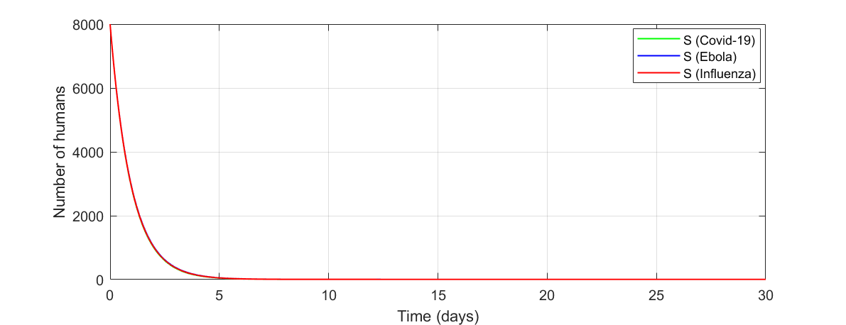
Figures 27 and 28 show that in the presence of controls, population susceptible to infection goes to zero in around five days. For exposed population in Ebola disease, their number increase before starting to decrease to zero because of the rate $k$. Unlike, for Covid-19 and Influenza, the number of exposed population decrease to zero quickly (in around $15$ days). For asymptomatic population, zeroing their number may take more time since there is no direct controls in this groups. It is the same for infected population even there is a direct control in this group, but this is not enough the fact that others population relocate this group away from asymptomatic and exposed groups. For recovered population, their number is smaller for Ebola disease than that for Covid-19 and influenza. This is acceptable because of the fatality rate of Ebola. Then, a few of them will recovered from of the virus when the rest of them will die because of the infection, even in the presence of controls.

8. Conclusion

In this paper, we have considered a SEIAR dynamic epidemic model adding new groups called vaccinated population ($V_{1}$, $\ldots$, $V_{n}$), denoted as (VS-EIAR). The aim was to control the propagation of the infection by decreasing the number of susceptible, exposed, asymptomatic, and infected populations using optimal control theory. Our strategy was based on two control actions: the first one involved vaccinating the population susceptible to the infection, and the second one involved providing treatment to those who are infected. The Pontryagin’s maximum principle (PMP) was used to establish the optimal controls and the finite optimal time. To make the study more relevant, we considered an impulsive dynamic pandemic model that accounts for immigration and travel. The impulsive VS-EIAR epidemic model can also be controlled using our control strategy. The theoretical analysis was complemented by numerical simulations to test the viability of our method for controlling the spread of Covid-19. Additionally, a comparison is provided to compare between three different diseases (Covid-19, Ebola, and Influenza) under both impulsive and non-impulsive scenarios.

Refer to caption
Figure 1. The VS-EIAR epidemic model without the impulsive rate of growth.
Refer to caption
Figure 2. The VS-EIAR epidemic model with the impulsive rate of growth.
Refer to caption
Figure 3. Changes in the vaccinated group without the impulsive rate of growth.
Refer to caption
Figure 4. Changes in the susceptible group without the impulsive rate of growth.
Refer to caption
Figure 5. Changes in the exposed group without the impulsive rate of growth.
Refer to caption
Figure 6. Changes in the asymptomatic group without the impulsive rate of growth.
Refer to caption
Figure 7. Changes in the infected group without the impulsive rate of growth.
Refer to caption
Figure 8. Changes in the recovered group without the impulsive rate of growth.
Refer to caption
Figure 9. Changes in the deceased group without the impulsive rate of growth.
Refer to caption
Figure 10. Changes in the total population without the impulsive rate of growth.
Refer to caption
Figure 11. Comparison between total population without the impulsive rate in the presence and absence of controls.
Refer to caption
Figure 12. Comparison between recovered and vaccinated population and a total of them with and without controls.
Refer to caption
Figure 13. Changes in the vaccinated group with the impulsive rate of growth.
Refer to caption
Figure 14. Changes in susceptible group with the impulsive rate of growth.
Refer to caption
Figure 15. Changes in exposed group with the impulsive rate of growth.
Refer to caption
Figure 16. Changes in the asymptomatic group with the impulsive rate of growth.
Refer to caption
Figure 17. Changes in the infected group with the impulsive rate of growth.
Refer to caption
Figure 18. Changes in the recovered group with the impulsive rate of growth.
Refer to caption
Figure 19. Changes in the deceased group with the impulsive rate of growth.
Refer to caption
Figure 20. Changes in the total population with the impulsive rate of growth.
Refer to caption
Figure 21. Comparison between total population with the impulsive rate in the presence and absence of controls.
Refer to caption
Figure 22. Comparison between recovered and vaccinated population and a total of them with and without controls.
Refer to caption
Refer to caption
Refer to caption
Refer to caption
Figure 23. Changes of ($S(t)$, $E(t)$, $A(t)$, $I(t)$) with the impulsive rate of growth in Ebola.
Refer to caption
Refer to caption
Refer to caption
Refer to caption
Figure 24. Changes of ($R(t)$, $V(t)$ $D(t)$, $N(t)$) with the impulsive rate of growth in Ebola.
Refer to caption
Refer to caption
Refer to caption
Refer to caption
Figure 25. Changes of ($S(t)$, $E(t)$, $A(t)$, $I(t)$) with the impulsive rate of growth in Influenza.
Refer to caption
Refer to caption
Refer to caption
Refer to caption
Figure 26. Changes of ($R(t)$, $V(t)$ $D(t)$, $N(t)$) with the impulsive rate of growth in Influenza.
Refer to caption
Refer to caption
Refer to caption
Refer to caption
Figure 27. Comparison in ($S(t)$, $E(t)$, $A(t)$, $I(t)$) with impulsive for Covid-19, Ebola, and Influenza.
Refer to caption
Refer to caption
Refer to caption
Refer to caption
Figure 28. Comparison in ($R(t)$, $V(t)$ $D(t)$, $N(t)$) with impulsive for Covid-19, Ebola, and Influenza.

9. Appendix

Proof of Theorem 2.1..

Let $x(t)=\left(S(t),E(t),A(t),I(t),R(t),D(t),V_{1}(t),\ldots,V_{n}(t)\right)^{T}$. Equation (2.1) can be written as follows:

$$\left\{\begin{array}[]{l}\dot{x}(t)=F(t,x(t)),\quad t\geq 0\\ x(0)=x_{0},\end{array}\right.$$ (9.1)

where $F(t,x(t))\equiv F(x(t),w(t))$ for $w(t)=(v(t),u(t))^{T}$ in which $F(t,\cdot)=\left(F_{1}(t,\cdot),\ldots,F_{n+6}(t,\cdot)\right)$ is defined on $\mathbb{R}^{n+6}$ by

$$\left.\begin{array}[]{l}F_{1}(t,y)=-(\beta[\varepsilon y_{2}+(1-q)y_{4}+\mu y_{3}]+\gamma_{1}v(t))y_{1},\\ \\ F_{2}(t,y)=\beta[\varepsilon y_{2}+(1-q)y_{4}+\mu y_{3}]y_{1}-ky_{2}+\sum\limits_{i=1}^{n-1}\delta_{i}y_{i},\\ \\ F_{3}(t,y)=(1-z)ky_{2}-\eta y_{3},\\ \\ F_{4}(t,y)=zky_{2}+(1-p)\eta y_{3}-fy_{4}-u(t)y_{4},\\ \\ F_{5}(t,y)=\alpha fy_{4}+u(t)y_{4}+p\eta y_{3},\\ \\ F_{6}(t,y)=(1-\alpha)fy_{4},\\ \\ F_{7}(t,y)=\gamma_{1}v(t)y_{1}-\gamma_{2}v(t)y_{7}-\delta_{1}y_{7}\\ \\ \left\{\begin{array}[]{l}F_{i+6}(t,y)=\gamma_{i}v(t)y_{i+5}-\gamma_{i+1}v(t)y_{i+6}-\delta_{i}y_{i+6},\\ \\ \text{for}\hskip 2.84544pti=2,3,\ldots,n-1,\end{array}\right.\\ \\ F_{n+6}(t,y)=\gamma_{n}v(t)y_{n+5},\end{array}\right.$$

for $t\geq 0$ and $y=(y_{1},\ldots,y_{n+6})\in\mathbb{R}^{n+6}_{+}$. To show that equation (9.1) have a unique solution defined on an interval $[0,t_{max})$ for $t_{max}\leq+\infty$, it is sufficient to show that equation:

$$x(t)=x_{0}+\displaystyle\int_{0}^{t}F(s,x(s))ds\hskip 2.84544pt\text{ for }\hskip 2.84544ptt\geq 0,$$ (9.2)

has a unique solution $x(\cdot)$ defined on $[0,t_{max})$. In fact, the function $t\to F(t,Y)$ is almost everywhere continuous on $\mathbb{R}^{+}$ for each $Y\in\mathbb{R}^{n+6}_{+}$. Since $Y\to F(t,Y)$ is $\mathcal{C}^{1}(\mathbb{R}^{n+6})$, it follows that $F(t,\cdot)$ is locally Lipschitz with respect to the second argument. As a consequence, there exists a unique function $x(\cdot)$ defined on an interval $[0,t_{max})$ for $t_{max}\leq+\infty$ that satisfy equation (9.2).

In the next, we demonstrate the positivity of solutions. For $S(t)$, it follows from equation (2.1) that

$$S(t)=\exp\left(-\int_{0}^{t}(\beta\Lambda(s)+\gamma_{1}v(s))ds\right)S(0)\quad\text{ for }\quad t\in[0,t_{\text{max}}).$$ (9.3)

Since $S(0)\geq 0$, we have $S(t)\geq 0$ for $t\in[0,t_{\text{max}})$.

For $V_{1}(t)$, it follows from equation (2.1) that

$$V_{1}(t)=R_{1}(t,0)V_{1}(0)+\gamma_{1}\int_{0}^{t}R_{1}(t,s)v(s)S(s)ds\quad\text{ for }\quad t\in[0,t_{\text{max}}),$$

where

$$R_{1}(t,s)=\exp\left(-\int_{s}^{t}(\delta_{1}+\gamma_{2}v(s))ds\right)\quad\text{ for }\quad 0\leq s\leq t<t_{\text{max}}.$$

Since $S(t)\geq 0$, $v(t)\geq 0$, and $V_{1}(0)\geq 0$, we conclude that $V_{1}(t)\geq 0$ for $t\in[0,t_{\text{max}})$.

For $V_{i}(t)$ with $i=2,\ldots,n-1$, we have

$$V_{i}(t)=R_{i}(t,0)V_{i}(0)+\gamma_{i}\int_{0}^{t}R_{i}(t,s)v(s)V_{i-1}(s)ds\quad\text{ for }\quad t\in[0,t_{\text{max}}),$$

where

$$R_{i}(t,s)=\exp\left(-\int_{s}^{t}(\delta_{i}+\gamma_{i+1}v(s))ds\right)\quad\text{ for }\quad 0\leq s\leq t<t_{\text{max}}.$$

Since $V_{i}(0)\geq 0$ and $V_{i-1}(t)\geq 0$ for $i=2,\ldots,n-1$, we have $v_{i}(t)\geq 0$ for $i=2,\ldots,n-1$.

For $E(t)$, $A(t)$, and $I(t)$, we can consider the following system:

$$\dot{X}(t)=BX(t)+G\left(X(t)\right),\quad t\geq 0$$ (9.4)

for $X(t)=(E(t),A(t),I(t))^{T}$, where

$$B=\begin{pmatrix}-k&0&0\\ (1-z)k&-\eta&0\\ zk&(1-z)\eta&-f\end{pmatrix}$$

and

$$G\left(X(t)\right)=\begin{pmatrix}\beta\Lambda(t)S(t)+\sum_{i=1}^{n-1}\delta_{i}V_{i}(t)\\ 0\\ -u(t)I(t)\end{pmatrix}$$

for $t\in[0,t_{\text{max}})$.

For $\lambda>0$, we can rewrite equation (9.4) as:

$$\dot{X}(t)=(B-\lambda I_{3})X(t)+G_{\lambda}(X(t))\quad\text{ for }\quad t\geq 0,$$ (9.5)

where $G_{\lambda}(X(t))=G(X(t))+\lambda X(t)$. Since $0\leq u(t)\leq 1$, for $\lambda>0$ sufficiently large, we have $G_{\lambda}(w)\geq 0$ for $w\geq 0$. From (9.5), we obtain:

X​(t)=exp⁑(t​(Bβˆ’Ξ»β€‹I3))​X​(0)+∫0texp⁑((tβˆ’s)​(Bβˆ’Ξ»β€‹I3))​Gλ​(X​(s))​𝑑sΒ forΒ t∈[0,tmax).formulae-sequenceπ‘‹π‘‘π‘‘π΅πœ†subscript𝐼3𝑋0superscriptsubscript0π‘‘π‘‘π‘ π΅πœ†subscript𝐼3subscriptπΊπœ†π‘‹π‘ differential-d𝑠 for 𝑑0subscript𝑑maxX(t)=\exp(t(B-\lambda I_{3}))X(0)+\int_{0}^{t}\exp((t-s)(B-\lambda I_{3}))G_{\lambda}(X(s))ds\quad\text{ for }\quad t\in[0,t_{\text{max}}).

Since $X(0)\geq 0$, it follows that $X(t)\geq 0$ for $t\in[0,t_{\text{max}})$.

For $R(t)$, we have

R​(t)=R​(0)+∫0t[α​f​I​(s)+u​(s)​I​(s)+p​η​A​(s)]​𝑑sΒ forΒ t∈[0,tmax).formulae-sequence𝑅𝑑𝑅0superscriptsubscript0𝑑delimited-[]π›Όπ‘“πΌπ‘ π‘’π‘ πΌπ‘ π‘πœ‚π΄π‘ differential-d𝑠 for 𝑑0subscript𝑑maxR(t)=R(0)+\int_{0}^{t}[\alpha fI(s)+u(s)I(s)+p\eta A(s)]ds\quad\text{ for }\quad t\in[0,t_{\text{max}}).

Since $R(0)\geq 0$, $I(t)\geq 0$, and $A(t)\geq 0$, we conclude that $R(t)\geq 0$ for $t\in[0,t_{\text{max}})$.

For $D(t)$, we have

$$D(t)=D(0)+(1-\alpha)f\int_{0}^{t}I(s)ds\quad\text{ for }\quad t\in[0,t_{\text{max}}).$$

Since $D(0)\geq 0$ and $I(t)\geq 0$ for $t\in[0,t_{\text{max}})$, we obtain $D(t)\geq 0$ for $t\in[0,t_{\text{max}})$.

Finally, we show the boundedness of solutions. Since $\dot{N}(t)=(\alpha-1)I(t)\leq 0$, it follows that $N(\cdot)$ is decreasing, which implies that $0\leq N(t)\leq N_{0}$ for $t\in[0,t_{max})$. Then, solutions of equation (2.1) are bounded. As a consequence $t_{max}=+\infty$. ∎

Proof of Theorem 3.2..

The optimal controls can be calculated by

$\nabla_{u(t)}^{H}=\dfrac{\partial H}{\partial u(t)}=0$  and $\nabla_{v(t)}^{H}=\dfrac{\partial H}{\partial v(t)}=0$.

Therefore,

$u^{*}(t)=\dfrac{I^{*}(t)\left[p_{4}(t)-p_{5}(t)\right]}{\sigma_{0}}$,

and

$v^{*}(t)=\dfrac{\left[\gamma_{1}S^{*}(t)[p_{1}(t)-q_{1}(t)]+\gamma_{2}q_{1}(t)V_{1}^{*}(t)+\sum\limits_{i=2}^{n-1}q_{i}(t)[\gamma_{i+1}V_{i}^{*}(t)-\gamma_{i}V^{*}_{i-1}(t)]\right]}{\left(\sum\limits_{i=1}^{n}\sigma_{i}\gamma_{i}^{2}\right)}$,

for $t\in[0,\tau^{*}]$. Since $u^{*}\in U_{ad}^{1}$ and $v^{*}\in U_{ad}^{2}$, it follows that

$$u^{*}(t)=\max\left\{\min\left\{\dfrac{I^{*}(t)\left[p_{4}(t)-p_{5}(t)\right]}{\sigma_{0}},1\right\},0\right\},$$

and

$$v^{*}(t)=\max\left\{\min\left\{\dfrac{W(t)}{\left(\sum\limits_{i=1}^{n}\sigma_{i}\gamma_{i}^{2}\right)},\dfrac{1}{\gamma_{1}}\right\},0\right\},$$

where

$W(t)=\dfrac{\left[\gamma_{1}S^{*}(t)[p_{1}(t)-q_{1}(t)]+\gamma_{2}q_{1}(t)V_{1}^{*}(t)+\sum\limits_{i=2}^{n-1}q_{i}(t)[\gamma_{i+1}V_{i}^{*}(t)-\gamma_{i}V^{*}_{i-1}(t)]\right]}{\left(\sum\limits_{i=1}^{n}\sigma_{i}\gamma_{i}^{2}\right)}$,

for $t\in[0,\tau^{*}]$. The optimal final time $\tau^{*}$ can be calculated by

$$H\left(X^{*}(\tau^{*}),v^{*}(\tau^{*}),u^{*}(\tau^{*}),P^{*}(\tau^{*}),Q^{*}(\tau^{*}),\tau^{*}\right)+\dfrac{\partial\mathcal{M}(\tau^{*})}{\partial t}=0.$$

The rest of the proof follows in (3.3)-(3.4). ∎

Proof of Theorem 4.1..

Let $x(t)=\left(S(t),E(t),A(t),I(t),R(t),D(t),V_{1}(t),\ldots,V_{n}(t)\right)^{T}$, and $\rho_{i}(\cdot)$ $(\text{for }i=1,\ldots,4)$ be the functions defined by

ρi​(t)={Ξ»i​(tk)​ if ​t=tk+0​ if ​tβ‰ tk+.subscriptπœŒπ‘–π‘‘casessubscriptπœ†π‘–subscriptπ‘‘π‘˜Β if 𝑑subscriptsuperscriptπ‘‘π‘˜0Β if 𝑑subscriptsuperscriptπ‘‘π‘˜\rho_{i}(t)=\left\{\begin{array}[]{l}\lambda_{i}(t_{k})\text{ if }t=t^{+}_{k}\\ 0\text{ if }t\neq t^{+}_{k}.\end{array}\right.

Equation (4.1) can be written as

$$\left\{\begin{array}[]{l}\dot{x}(t)=L(t,x(t)),\quad t\geq 0\\ x(0)=x_{0},\end{array}\right.$$ (9.6)

where $L(t,\cdot)=\left(L_{1}(t,\cdot),\ldots,L_{n+6}(t,\cdot)\right)$ is defined on $\mathbb{R}^{n+6}$ by

$$L_{i}(t,y)=\left\{\begin{array}[]{l}F_{i}(t,y)+\rho_{i}(t)y_{i}\hskip 2.84544pt\text{ for }\hskip 2.84544pti=1,\ldots,4,\\ F_{i}(t,y)\hskip 2.84544pt\text{ for }\hskip 2.84544pti=5,\ldots,n+6,\end{array}\right.$$

for $t\geq 0$ and $y=(y_{1},\ldots,y_{n+6})\in\mathbb{R}^{n+6}_{+}$. The function $t\to L(t,Y)$ is locally $\mathbb{L}^{1}-$integrable on $\mathbb{R}^{+}$ for each $Y\in\mathbb{R}^{n+6}_{+}$. Since $L(t,\cdot)$ is $\mathcal{C}^{1}(\mathbb{R}^{n+6})$, it follows that $L(t,\cdot)$ is Locally Lipschitz. As a consequence, equation (9.6) have a unique solution $x(\cdot)$ defined on an interval $[0,t_{max})$ for $t_{max}\leq+\infty$, and satisfying the following integral equation:

$$x(t)=x_{0}+\displaystyle\int_{0}^{t}L(s,x(s))ds\hskip 2.84544pt\text{ for }\hskip 2.84544ptt\in[0,t_{max}).$$

To show the positivity of solutions, we follow the same approach as presented in the proof of Theorem 2.1. Finally, we show the boundedness of solutions and $t_{max}=+\infty$. For this reason, we discuses the following cases:

  1. case 1: if $t_{max}<t_{1}$, we have $\dot{N}(t)=(\alpha-1)I(t)\leq 0$ for $t\in[0,t_{max})$, then $N(t)\leq N_{0}$ for $t\in[0,t_{max})$.

  2. case 2: if $t_{max}\in[t_{1},t_{2}[$, we have $\dot{N}(t)=(\alpha-1)I(t)\leq 0$ for $t\in[0,t_{1}[$, then $N(t)\leq N_{0}$ for $t\in[0,t_{1}[$. If $t=t_{1}$, we have $N(t_{1})=N(t_{1}^{-})+N(t_{1}^{+})-N(t_{1}^{-})\leq N_{0}+\left[N(t_{1}^{+})-N(t_{1}^{-})\right]$. Then, $N(t)\leq N_{0}+\left[N(t_{1}^{+})-N(t_{1}^{-})\right]$ for $t\in[0,t_{1}]$. If $t\in]t_{1},t_{max})$, we have $\dot{N}(t)=(\alpha-1)I(t)\leq 0$, then $N(t)\leq N(t_{1})\leq N_{0}+\left[N(t_{1}^{+})-N(t_{1}^{-})\right]$ for $t\in[t_{1},t_{max})$. As a consequence, in that case, $N(t)\leq N_{0}+\left[N(t_{1}^{+})-N(t_{1}^{-})\right]$ for $t\in[0,t_{max})$.

  3. case 3: without loss of generality, we can assume that $t_{max}>t_{p}$. For $t\in]t_{1},t_{2}[$, we have $\dot{N}(t)=(\alpha-1)I(t)\leq 0$, then $N(t)\leq N(t_{1})\leq N_{0}+\left[N(t_{1}^{+})-N(t_{1}^{-})\right]$. If $t=t_{2}$, we have $N(t_{2})=N(t_{2}^{-})+N(t_{2}^{+})-N(t_{2}^{-})\leq N(t_{1})+\left[N(t_{2}^{+})-N(t_{2}^{-})\right]$. Hence, $N(t)\leq N_{0}+\sum\limits_{i=1}^{2}\left[N(t_{i}^{+})-N(t_{i}^{-})\right]$ for $t\in[0,t_{2}]$. Similarly, we obtain $N(t)\leq N_{0}+\sum\limits_{i=1}^{p}\left[N(t_{i}^{+})-N(t_{i}^{-})\right]$ for $t\in[0,t_{max})$.

We conclude that solutions of equation (4.1) are bounded and must be defined on $\mathbb{R}^{+}$, implying that $t_{max}=+\infty$. ∎

Financial disclosure

The authors declare that they have no known competing financial interests or personal relationships that could have appeared to influence the work reported in this paper.

Conflict of interest

This work does not have any conflicts of interest.

References

  • [1] World Health Organization, Coronavirus disease 2019 (Covid-19): situation report, 99, 2020.
  • [2] Z. Abbasi, I. Zamani, A. H. Amiri Mehra, Mohsen Shafieirad, Asier Ibeas, Optimal Control Design of Impulsive SQEIAR Epidemic Models with Application to Covid-19, Chaos, Solitons & Fractals, Volume 139, 2020, 110054.
  • [3] C. L. Althaus. Estimating the reproduction number of Ebola virus (EBOV) during the 2014 outbreak in West Africa. PLoS currents, 2014, vol. 6.
  • [4] S. I. Araz. Analysis of a Covid-19 model: optimal control, stability and simulations. Alexandria Engineering Journal, 2021, vol. 60, no 1, p. 647-658.
  • [5] J. Arino, F. Brauer, P. V. D. Drissche, et al. A model for influenza with vaccination and antiviral treatment. Journal of theoretical biology, 2008, vol. 253, no 1, p. 118-130.
  • [6] J. K. K. Asamoah, E. Okyere, A. Abedimi, et al. Optimal control and comprehensive cost-effectiveness analysis for Covid-19. Results in Physics, 2022, vol. 33, p. 105177.
  • [7] E. M. Aquino, I. H. Silveira, J. M. Pescarini, et al. Social distancing measures to control the Covid-19 pandemic: potential impacts and challenges in Brazil. Ciencia & saude coletiva, 2020, vol. 25, p. 2423-2446.
  • [8] D. Bainov, D. D. Bainov, and P. S. Simeonov. Systems with impulse effect: stability, theory, and applications. Ellis Horwood, 1989.
  • [9] D. Bainov, and P. Simeonov. Impulsive differential equations: periodic solutions and applications. Vol. 66. CRC Press, 1993.
  • [10] M. Benchohra, J. Henderson, and S. Ntouyas. Impulsive differential equations and inclusions. Vol. 2. New York: Hindawi Publishing Corporation, 2006.
  • [11] M. De La Sen, R. P. Agarwal, A. Ibeas, et al. On a generalized time-varying SEIR epidemic model with mixed point and distributed time-varying delays and combined regular and impulsive vaccination controls. Advances in Difference Equations, 2010, vol. 2010, p. 1-42.
  • [12] N. G. Davies, P. Klepac, Y. Liu, et al. Age-dependent effects in the transmission and control of Covid-19 epidemics. Nature medicine, 2020, vol. 26, no 8, p. 1205-1211.
  • [13] H. R. Guner, I. Hasanglu, and F. Aktas. Covid-19: Prevention and control measures in community. Turkish Journal of medical sciences, 2020, vol. 50, no 9, p. 571-577.
  • [14] J. Hui, and L. Chen. Impulsive vaccination of SIR epidemic models with nonlinear incidence rates. Discrete & Continuous Dynamical Systems-B, 2004, vol. 4, no 3, p. 595.
  • [15] V. Lakshmikantham, and P. S. Simeonov. Theory of impulsive differential equations. Vol. 6. World scientific, 1989.
  • [16] G. B. Libotte, S. F. Lobato, G. M. Platt, et al. Determination of an optimal control strategy for vaccine administration in Covid-19 pandemic treatment. Computer methods and programs in biomedicine, 2020, vol. 196, p. 105664.
  • [17] Q. Li, X. Guan, P. Wu et al. Early transmission dynamics in Wuhan, China, of novel coronavirus–infected pneumonia. New England journal of medicine, 2020.
  • [18] S. M. Moghadas, M. C. Fitzpatrick, P. Sah, et al. The implications of silent transmission for the control of Covid-19 outbreaks. Proceedings of the National Academy of Sciences, 2020, vol. 117, no 30, p. 17513-17515.
  • [19] S. Nana-Kyere, F. A. Boateng, P. Jonathan, et al. Global Analysis and optimal control model of Covid-19. Computational and Mathematical Methods in Medicine, 2022, vol. 2022.
  • [20] Y. Jin, H. Yang, W. JI, and al. Virology, epidemiology, pathogenesis, and control of Covid-19. Viruses, 2020, vol. 12, no 4, p. 372.
  • [21] T. A. Perkins and G. Espana. Optimal control of the Covid-19 pandemic with non-pharmaceutical interventions. Bulletin of mathematical biology, 2020, vol. 82, no 9, p. 1-24.
  • [22] J. Riou, and C. L. Althaus. Pattern of early human-to-human transmission of Wuhan 2019 novel coronavirus (2019-nCoV), December 2019 to January 2020. Eurosurveillance, 2020, vol. 25, no 4, p. 2000058.
  • [23] A. M. Samoilenko, and N. A. Perestyuk. Impulsive differential equations. world scientific, 1995.
  • [24] Z. H. Shen, Y. M. Chu, M. A. Khan, et al. Mathematical modeling and optimal control of the Covid-19 dynamics. Results in Physics, 2021, vol. 31, p. 105028.
  • [25] M. Zamir, Z. Shah, F. Nadeem, et al. Non pharmaceutical interventions for optimal control of Covid-19. Computer methods and programs in biomedicine, 2020, vol. 196, p. 105642.
  • [26] S. Zhao, et H. Chen. Modeling the epidemic dynamics and control of Covid-19 outbreak in China. Quantitative biology, 2020, vol. 8, no 1, p. 11-19.
  • [27] L. Wang, L. Chen, and J. J. Nieto. The dynamics of an epidemic model for pest control with impulsive effect. Nonlinear Analysis: Real World Applications, 2010, vol. 11, no 3, p. 1374-1386.