Scalable tomography of many-body quantum environments with low temporal entanglement

Abstract

Describing dynamics of a quantum system coupled to a complex many-body environment is a ubiquitous problem in quantum science. General non-Markovian environments are characterized by their influence matrix (IM) – a multi-time tensor arising from repeated interactions between the system and environment. While complexity of the most generic IM grows exponentially with the evolution time, recent works argued that for many instances of physical many-body environments, the IM is significantly less complex. This is thanks to area-law scaling of temporal entanglement, which quantifies the correlations between the past and the future states of the system. However, efficient classical algorithms for computing IM are only available for non-interacting environments or certain interacting 1D environments. Here, we study a learning algorithm for reconstructing IMs of large many-body environments simulated on a quantum processor. This hybrid algorithm involves experimentally collecting quantum measurement results of auxiliary qubits which are repeatedly coupled to the many-body environment, followed by a classical machine-learning construction of a matrix-product (MPS) representation of the IM. Using the example of 1D spin-chain environments, with a classically generated training dataset, we demonstrate that the algorithm allows scalable reconstruction of IMs for long evolution times. The reconstructed IM can be used to efficiently model quantum transport through an impurity, including cases with multiple leads and time-dependent controls. These results indicate the feasibility of characterizing long-time dynamics of complex environments using a limited number of measurements, under the assumption of a moderate temporal entanglement.

I Introduction

Rapid experimental progress opened up a new era in which quantum processors are increasingly capable of performing tasks that are challenging for classical computers [1, 2, 3]. One notable example of such a task, which received much attention, is the problem of random circuit sampling [4, 5]. The advent of powerful quantum processors calls both for further advances of classical computational methods, and for identifying applications that are beyond the reach of classical computers.

Non-equilibrium phenomena in quantum many-body systems [6, 7, 8, 9] are a promising class of such applications, because dynamics often leads to rapid growth of entanglement and computational complexity of system’s wave function [3]. Traditional tensor-network methods [10, 11], efficient for ground states which typically feature low, area-law entanglement, therefore generally struggle [12, 13, 14] to describe non-equilibrium phenomena such as evolution following quantum quenches and quantum transport, although notable advances were made for 1d systems [15].

Recently, a new family of methods for quantum many-body dynamics, based on compact matrix product state (MPS) representations of the influence matrix (IM) – a generalized version of the Feynman-Vernon influence functional – has emerged [16, 17, 18, 19, 20, 21]. These methods are suitable for computing dynamics of local physical observables, and, in contrast to more conventional tensor-network techniques, their efficiency rests on moderate temporal entanglement (TE) of the IM, which may be significantly lower than spatial entanglement [16, 17, 22]. These and related ideas, in particular, led to new efficient methods for bosonic [23, 24, 25, 26] and fermionic [27, 28, 29] quantum impurity models (QIM) out-of-equilibrium. An important class of QIM includes models of a small quantum system coupled to a bath of (possibly infinitely) many non-interacting degrees of freedom. Spin-boson QIMs are paradigmatic model for studying non-Markovian dynamics. Fermionic QIMs have important applications in quantum transport in mesoscopic systems [30, 31], and in dynamical mean-field theory methods for modelling strongly correlated materials [32, 33]. A schematic of a QIM arising in a transport setup with two environments is illustrated in Fig. 1a.

Intuitively, moderate TE in QIM and some other non-equilibrium settings is due to the fact that some of the information about the state of the impurity propagates into the environment without affecting the future dynamics of the impurity. This allows representing the environment with many degrees of freedom in a much more compact form, by an evolution of a finite-dimensional environment subject to Markovian dissipation, corresponding to irreversible information loss (see Fig. 1b).

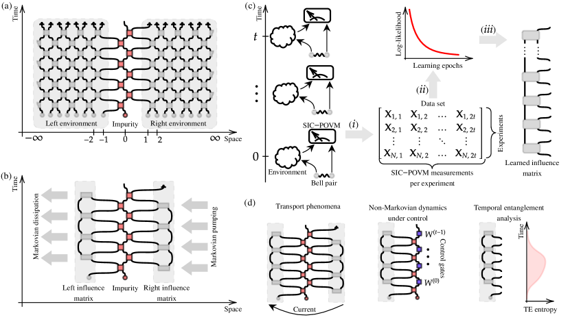
Figure 1: (a) A tensor network diagram representing discretized dynamics of an impurity (red shaded area) connecting to two infinite one-dimensional reservoirs (environments). A particular example of reservoir considered below is an XX spin chain that maps onto free spinless fermions. Grey shaded parts of the diagram represent influence matrices of the environments. (b) A tensor network diagram approximating the same impurity dynamics, but effective compressed IMs. Dimensionality reduction is achieved by elimination of environment degrees of freedom which do not affect the impurity time evolution. (c) Key steps of the IM learning procedure: (i) a data set is collected, by performing measurements on auxiliary degrees of freedom repeatedly interacting with an environment; (ii) the data set is used by the learning algorithm that finds IM MPS ansatz matching the given data set the best; (iii) A reconstructed MPS approximation of an IM is obtained, enabling numerical simulations of QIM dynamics. (d) A schematic illustration of example applications of the learned IM, in particular: transport phenomena simulation, such as a current flow in QIIM; non-Markovian dynamics simulation under external control; temporal entanglement analysis.

In another notable line of developments, a framework for describing non-Markovian dynamics in terms of a process tensor (PT) – a multi-time generalization of a quantum channel – has been developed [34]. Among other applications, the PT, which is formally equivalent to the IM, was applied to define measures of non-Markovianity [35], and to characterize quantum devices by performing PT tomography from experimental data [36, 37].

In this article, building on this recent progress, we propose to apply quantum processors to the problem of constructing the IM of complex quantum many-body environments. The schematic of the hybrid quantum-classical algorithm is illustrated in Fig. 1c. Conceptually, its key steps are: (i) collecting measurement results of probe qubits (or ancilla qubits), which are repeatedly coupled to an evolving quantum many-body system, the environment; (ii) feeding the collected data set to a machine-learning algorithm which constructs an MPS representation for the IM that matches the measurement results best according to the log–likelihood function; (iii) using the resulting IM to predict dynamics involving a given environment, e.g. as a reservoir in a QIM.

We study the applicability of this hybrid approach for for reconstructing IM of infinite quantum many-body environments at long evolution times. We note that previous works [38, 36, 37] investigated PT learning using a number of approaches, with some of those approaches exhibiting an exponential overhead in the number of evolution time steps, which precludes their scalability in the evolution time. However, under the assumption of a finite Markov order of the PT which leads to a finite bond dimension in the MPS ansatz for the IM, efficiency can be significantly improved. Closest in spirit to the present work, Ref. [39] explored MPS-based tomography [40] of PT for interacting environments of up to 6 interacting spins.

To assess the feasibility of learning the IM of quantum many-body environments, we consider environments that are semi-infinite spin chains. The training data for such environments are obtained using recently developed efficient classical algorithms [18, 21], yielding an accurate MPS representation of the IM for a large number of time-evolution steps. As a key result, we demonstrate that the learning procedure is scalable: in particular, we reconstruct IMs of several spin chains in the thermodynamic limit for $60$ discrete time steps that correspond to an IM with as many as $2^{240}$ entries. Reconstruction of such IMs requires millions of samples, which are accessible with current quantum hardware such as superconducting qubit processors [4, 5].

While here we generate the dataset classically, this approach will be most useful for many-body environments where no classical algorithm to compute IM exists, but temporal entanglement is sufficiently low, thus allowing for an approximation of an IM using MPS with a moderate bond dimension. Indeed, recent works argued that the area-law temporal entanglement scaling is a generic feature of systems with quasiparticles [21], including interacting integrable systems [41]. However, efficient algorithm for computing IM in such interacting systems are only available for one-dimensional systems. In a large variety of many-body phases, low-energy excited states can be effectively described by quasiparticle excitations. Thus, we expect the IM-learning to be applicable to such systems, in higher dimensions and varying system geometry.

Once an MPS representation of an IM of a complex many-body environment has been constructed, the dynamics of the QIM with that environment can be efficiently analyzed classically, as illustrated in Fig. 1d. Crucially, once an IM has been learned, QIM dynamics for arbitrary impurity parameters (e.g. on-site interaction) and time-dependent controls become accessible. Below we demonstrate this by reconstructing an IM of XX and XXX semi-infinite spin chains, and using it to simulate several relevant examples of impurity dynamics, including (i) non-Markovian effects in dynamics of impurity under external controls; (ii) quantum transport through the impurity connected to two reservoirs, whose IMs are learned separately.

The paper is structured as follows: In Sec. II we introduce the influence matrix formalism as a way to compute local observables dynamics and transport properties of many-body quantum systems. Further, we describe the influence matrix learning method in Sec. III. Next we discuss numerical results confirming the capabilities of the proposed method in Sec. IV. Finally we discuss the results, challenges and further development of the method in Sec. V.

II Influence matrix

Figure 2: (a) A tensor network diagram representing the dynamics of $\langle O(t)\rangle$, an observable of an impurity coupled with an environment. This diagram corresponds to the right-hand side of Eq. (4), with a shaded area highlighting the IM of an environment $\mathcal{J}_{\{j_{\tau},i_{\tau}\}_{\tau=0}^{t-1}}$ (see Eq. (6)). Below the main tensor network diagram is a schematic representation of an impurity interacting with an environment. (b) A tensor network diagram representing the dynamics of $\langle O(t)\rangle$ in a quantum transport setting. Here, $O$ is an observable of the left component of a two-qubit impurity coupled with two different environments. The superscripts $\mathcal{J}^{L}$ and $\mathcal{J}^{R}$ refer to the left and right environments, respectively.

We start by reviewing the influence matrix framework [17] (see also closely related PT formalism [34]). The IM is a multi-time tensor that contains complete information regarding the effect of the environment on impurity dynamics. Formally, it can be obtained by integrating out environment degrees of freedom. The complexity of the IM can be significantly lower than the complexity of the combined impurity-environment wave function, since not all the information regarding the internal state of environment is retained. This allows for compact representations of IM in a number of non-equilibrium settings [16, 17, 22, 18, 19, 20, 21].

To define the IM, consider a QIM, where an impurity is a small quantum system described by a finite-dimensional local Hilbert space, while an environment is a many-body, possibly infinite-dimensional quantum system. We describe the state of the impurity-environment system by a vectorized time-dependent density matrix $\rho_{i\alpha}(t)$ (see Appendix A for further details on the vectorization). The first index refers to the impurity degrees of freedom and the second index refers to the environment degrees of freedom. For brevity of notation, we use Einstein’s summation convention in what follows. Our goal is to study the dynamics of the impurity by integrating out the environment’s degrees of freedom. Thus, we are interested in expectation values of the following form:

$$\left\langle O(t)\right\rangle=O_{i}\mathds{1}_{\alpha}\rho_{i\alpha}(t),$$ (1)

where $O_{i}$ is a vectorized operator of a local observable $\hat{O}$ on the impurity and $\mathds{1}_{\alpha}$ is the vectorized identity operator that acts on the environment degrees of freedom as the partial trace. The initial state of the composite system $\rho_{i\alpha}(0)$ is taken to be a product state between the initial state of the impurity $\rho^{I}_{i}$ and the environment $\rho^{E}_{\alpha}$

$$\rho_{i\alpha}(0)=\rho^{I}_{i}\rho^{E}_{\alpha}.$$ (2)

We consider discrete time evolution of the composite system, which naturally arises when the continuous time evolution of the QIM, defined by a Hamiltonian or a Lindbladian, is discretized (trotterized). It is convenient to decompose each time step of the evolution into two half-steps. The first half-step, described by a quantum channel $V_{i\alpha,j\beta}$, represents an evolution step due to environment’s own dynamics, as well as due to the system-environment interaction (see Fig. 2). For simplicity, we consider a time-translation invariant evolution of the environment, hence $V$ is constant (a generalization to the case when $V$ is time-dependent is straightforward). During the second half-step of the evolution, quantum channels $W^{(t)}_{i,j}$ that act only on the impurity, are applied. We consider time-dependent $W^{(t)}$ since we allow an arbitrary control signal applied to the impurity. Thus, density matrix dynamics evolution over one step reads

$$\rho_{i\alpha}\left(t+\frac{1}{2}\right) =V_{i\alpha,i^{\prime}\alpha^{\prime}}\rho_{i^{\prime}\alpha^{\prime}}(t),$$

$$\rho_{i\alpha}(t+1) =W^{(t)}_{i,i^{\prime}}\rho_{i^{\prime}\alpha}\left(t+\frac{1}{2}\right).$$ (3)

Integrating Eq. (3) forward in time and substituting the integration result into Eq. (1), we express the dynamics of the impurity observable as follows,

$$\left\langle O(t)\right\rangle =O_{i_{t}}\mathds{1}_{\alpha_{t}}\left(\prod_{\tau=1}^{t}W^{(\tau-1)}_{i_{\tau}j_{\tau-1}}V_{\alpha_{\tau}j_{\tau-1},\alpha_{\tau-1}i_{\tau-1}}\right)$$ (4)

$$\times\rho^{E}_{\alpha_{0}}\rho^{I}_{i_{0}}.$$

It is convenient to represent the right part of Eq. (4) in terms of a tensor network diagram, as illustrated in Fig. 2a. Further, we rewrite Eq. (4) as

$$\left\langle O(t)\right\rangle=\mathcal{J}_{\{j_{\tau},i_{\tau}\}_{\tau=0}^{t-1}}O_{i_{t}}\left(\prod_{\tau=0}^{t-1}W^{(\tau)}_{i_{\tau+1}j_{\tau}}\right)\rho^{I}_{i_{0}},$$ (5)

where the IM $\mathcal{J}_{\{j_{\tau},i_{\tau}\}_{\tau=0}^{t-1}}$ is defined as follows,

$$\mathcal{J}_{\{j_{\tau},i_{\tau}\}_{\tau=0}^{t-1}}=\mathds{1}_{\alpha_{t}}\left(\prod_{\tau=0}^{t-1}V_{\alpha_{\tau+1}j_{\tau},\alpha_{\tau}i_{\tau}}\right)\rho^{E}_{\alpha_{0}}.$$ (6)

This IM is a generalization of a Feynman-Vernon influence functional [42]. In Fig. 2a we highlight IM’s tensor diagram by the shaded area. The IM encapsulates all the effects of the environment on an impurity, including dissipation and memory (non-Markovianity) of the environment. One advantage of the IM approach is that it allows one to describe arbitrary local impurity dynamics. In particular, arbitrary control sequences can be applied by selecting the channels $W^{(\tau)}$ which act on the impurity, since they are not included in the IM.

We can view Eq. (6) as an MPS representation of the IM. The quantum channels $V$ take the role of MPS tensors, and the dimension of the environment density matrix becomes the bond dimension. This suggests that conventional MPS compression algorithms such as singular value decomposition-based truncation [10] may be used to approximate an IM by an MPS with a lower bond dimension, effectively reducing the dimensionality of environment. An IM can be efficiently compressed provided its temporal entanglement – the entanglement entropy of the IM viewed as a wavefunction in the time domain – is moderate. It was found that for a wide variety of physically interesting cases, TE grows slowly with evolution time. This includes quantum circuits that are nearly dual unitary [17], many-body localized systems [43], dissipative systems [18], free fermion systems [27, 28], integrable systems [22, 41] and spin-boson models [26]. Additionally TE generally remains low in proximity to those regimes [17]. Using a compressed, low bond-dimension approximation of an IM, evolution of local observables can be efficiently computed, see Eq. (4).

Below we will be interested in analyzing transport through an impurity connecting two environments (left and right environments, see Fig. 2b). For concreteness, we choose a two-site impurity where the left environment only couples to the left site of the impurity and the right environment only couples to the right site of the impurity. The corresponding tensor diagram for observable dynamics in this model $\left\langle O(t)\right\rangle$ is illustrated in Fig. 2b. Note that left and right IMs enter the tensor network in Fig. 2b independently. This allows us to construct compressed IMs for the left and right environment independently and later combine them to build the more complex full environment. In the same fashion, multiple IMs can be combined [25].

The case where observable $\hat{O}$ corresponds to a conserved charge is of particular interest for transport properties. To compute the instantaneous current flowing between left and right parts of the impurity $I(t)$, we generalize Eq. (3) and Eq. (1) to an impurity coupled to a left and right environment. The generalization of Eq. (3) reads

$$\rho_{ik\alpha\beta}\left(t+\frac{1}{2}\right) =V_{i\alpha,i^{\prime}\alpha^{\prime}}^{L}\rho_{i^{\prime}k^{\prime}\alpha^{\prime}\beta^{\prime}}(t)V_{k\beta,k^{\prime}\beta^{\prime}}^{R},$$

$$\rho_{ik\alpha\beta}(t+1) =W_{ik,i^{\prime}k^{\prime}}^{(t)}\rho_{i^{\prime}k^{\prime}\alpha\beta}\left(t+\frac{1}{2}\right),$$ (7)

where indices $i,\ k$ of $\rho_{ik\alpha\beta}$ correspond to the impurity degrees of freedom, index $\alpha$ to the left environment degrees of freedom and index $\beta$ to the right environment degrees of freedom, $V^{R}$ and $V^{L}$ are quantum channels forming left and right IMs correspondingly. The generalization of Eq. (1) reads

$$\left\langle O(t)\right\rangle=O_{i}\mathds{1}_{k}\mathds{1}_{\alpha}\mathds{1}_{\beta}\rho_{ik\alpha\beta}(t),$$ (8)

assuming that we consider an observable of the left component of the impurity. Eqs. (7),(8) allow us to calculate a current $I(t)$ as a finite difference of a charge $O$ before and after the action of $W$, i.e.

$$I(t)=\left\langle O\left(t+1\right)\right\rangle-\left\langle O\left(t+\frac{1}{2}\right)\right\rangle.$$ (9)

For bounded observables and time independent dynamics we expect that the system reaches a steady state, and the long-time averages of the left and right current are equal to the steady-state current,

$$\overline{I(t)}=I_{s}.$$ (10)

The latter can be calculated as a long time asymptotic of Eq. (9). Replacing the original IMs by their compressed MPS representations makes this approach computationally efficient.

The efficiency of the approach described above hinges on obtaining a compressed, low bond dimension MPS representation of the IM. While low TE guarantees the existence of such an MPS, finding it for large environments can be challenging. The known cases where an MPS representation of system’s IM can be efficiently constructed classically include: (i) Interacting one-dimensional chains, via transversal contraction schemes [16, 21, 20]; (ii) Non-interacting bosons, which allow for explicit construction of a low bond dimension MPS representation using a finite memory time cutoff [23] or using auxiliary bosons [26]; (iii) Free fermions where IM can be expressed in terms of Gaussian integrals which are converted to MPS form [28, 29]. Despite these advances, there are important cases, such as interacting models in higher dimensions, where no algorithms to obtain the compressed IM are known.

Moreover, the following simple argument shows that the generic problem of computing the IM from a quantum circuit description of the environment is classically hard, even if restricted to IMs with low TE. To illustrate this, let us take an environment which is disconnected from the impurity qubit for the first $t-1$ steps of evolution. The degrees of freedom of the environment evolve according to a quantum circuit encoding a classically hard quantum computation, with an output written to the state of one of the environment’s qubits. At the last step, the state of this qubit is swapped with a qubit in the impurity. The corresponding IM is a product state and hence has zero TE, yet obtaining it requires simulating an arbitrary quantum computation.

III Influence matrix reconstruction from quantum measurements

Figure 3: (a) Illustration of the first protocol of data acquisition. At each time step a Bell pair depicted as $\ket{\Phi^{+}}\bra{\Phi^{+}}$ is prepared, and one of the qubits is coupled to the environment. The resulting quantum state, proportional to the environment’s IM, can be characterized by measuring qubits in different bases. In this scheme, measurements and evolution can be parallelized. (b) Illustration of a coarse grained protocol, where an ancilla interacts with the environment over two time steps. (c) Illustration of the second protocol, which requires one ancilla. At each step, the ancilla is prepared in an infinite temperature state depicted as $\frac{1}{2}\mathds{1}$, measured using a SIC-POVM, coupled to the environment before being measured again. This protocol provides the same statistics of measurements outcomes.

In this Section, we formulate a hybrid quantum-classical approach to learning the IM, building on previous works on PT tomography [39, 37]. The aim of this approach is to reconstruct a compressed approximation of a complex environment’s IM with moderate TE, in cases where no classical algorithm is readily available, e.g. for interacting environments in $d\geq 2$ dimensions.

At the first step, an experiment with a quantum computing device is performed: a quantum environment $E$ is simulated, probe qubits are brought to interact with $E$ at different times, and a set of measurements is performed, as described below. In the second, ‘classical‘ stage we use a likelihood maximization based reconstruction method to convert those measurement results into a low bond dimension MPS representation of the IM.

Below we discuss two alternative implementations of the first step, which differ in the way ancilla qubits are used. Both schemes sample the same probability distribution and are therefore equivalent from the theory perspective. However, they have different requirements in terms of the number of ancilla qubits and the measurement capabilities of the device; thus, one of the schemes may be better suited for a given experimental platform.

In the first implementation, multiple ancilla qubits are used to prepare a quantum state whose density matrix is proportional to the IM. Effectively, this quantum state is the Choi state [44, 45, 34] of the IM viewed as a quantum channel between $t$ input and $t$ output states. This implementation is illustrated in Fig. 3a: at each step, a Bell pair of ancilla qubits is prepared and one qubit of the pair interacts with $E$ over one time step. We repeat this procedure for each time step, preparing a state of $2t$ ancilla qubits. The density matrix of this state is equal to the IM, up to a normalization constant. Next, a symmetric, informationally complete positive operator-valued (SIC-POVM) measurement on each ancilla qubit is performed (see Appendix B for details). Each SIC-POVM measurement yields one of the 4 different possible SIC-POVM elements $\{M^{\alpha}\}_{\alpha=0}^{3}$, generating a string of $2t$ integer indices $\{0,1,2,3\}$ identifying a particular SIC-POVM element. This ‘asynchronous’ approach requires $2t$ ancilla qubits, and the measurement of a given auxiliary pair can be performed at any moment after the interaction with the environment. It allows one to parallelize evolution and measurements of each qubit – a potential advantage for platforms where measurements are significantly slower than unitary evolution.

In contrast to the first asynchronous approach, the second, fully sequential approach requires only one ancillary qubit that is measured multiple times. This implementation is schematically illustrated in Fig. 3c: At each step of time evolution, the ancilla qubit is (i) initialized in an infinite temperature state; (ii) a SIC-POVM on the ancilla is performed; the qubit is coupled to the environment for one time evolution step, and, finally (iv) another SIC-POVM is performed on the impurity qubit. After $t$ steps of time evolution we obtain a measurement string of length $2t$. This approach does not require multiple ancilla qubits, but one needs to alternate the environment time evolution with SIC-POVM measurements.

To reconstruct the IM from measurements, the experiment is repeated $N\gg 1$ times. We organize the measurement strings into a dataset matrix $\mathbf{X}_{k,l}$ where $k$ runs over $N$ strings and $l$ runs over the $2t$ individual SIC-POVM results in each string. In order to access the information about longer time scales with fewer samples it may be advantageous to perform measurements after two or more steps of ancilla-bath interaction. This is illustrated in Fig. 3b, where the ancilla is measured after two steps of interaction with $E$. We use such coarse graining procedure in some of our numerical experiments; more information about coarse graining is provided in Appendix D.

In the ‘classical‘ part of the algorithm we reconstruct a MPS representation of the IM from the set of measurement strings obtained in the quantum part. As established above, many relevant quantum environments have low TE and can hence be described by relatively few degrees of freedom even for a large number of time steps. To take advantage of this property, we use a low bond dimension ansatz and “learn” its parameters from the measurement results. The bond dimension is seen as a hyperparameter of the learning algorithm and can be tuned to regulate the upper bound of TE. Our ansatz is structurally identical to Eq. (6) and reads

$$\mathcal{J}_{\{j_{\tau},i_{\tau}\}_{\tau=0}^{t-1}}(\Theta,\rho)=\mathds{1}_{\alpha_{t}}\left(\prod_{\tau=0}^{t-1}\Theta_{\alpha_{\tau+1}j_{\tau},\alpha_{\tau}i_{\tau}}\right)\rho_{\alpha_{0}},$$ (11)

where $\Theta$ is an unknown quantum channel and $\rho$ is an unknown density matrix. To find the free parameters $\Theta$ and $\rho$, we maximize a logarithmic likelihood function of the dataset $\mathbf{X}_{k,l}$ with respect to those unknown parameters. The logarithmic likelihood function reads

$$\mathcal{L}(\mathbf{X},\Theta,\rho) =\sum_{k=1}^{N}\log\Bigg{(}\mathcal{J}_{\{j_{\tau},i_{\tau}\}_{\tau=0}^{t-1}}(\Theta,\rho)$$

$$\times\prod_{\tau=0}^{t-1}M_{j_{\tau}}^{\mathbf{X}_{k,2\tau+2}}M_{i_{\tau}}^{\mathbf{X}_{k,2\tau+1}}\Bigg{)}-2tN\log(2).$$ (12)

Here $\{M_{i}^{\alpha}\}_{\alpha=0}^{3}$ is a SIC-POVM with vectorized elements, where $\alpha$ runs over all elements and $i$ runs over all entries of a particular element. The last term in the r.-h.s. of Eq. (12), $2tN\log(2)$, is a normalization constant that can be safely omitted. The optimization problem that yields the most likely parameters $\Theta$ and $\rho$ can therefore be summarized as follows,

$$\underset{\Theta,\rho}{\rm maximize}\quad\mathcal{L}(\mathbf{X},\Theta,\rho)$$

$${\rm subject\ to}\quad\Theta\in{\rm CPTP},\ {\rm Tr}(\rho)=1,\ \rho\geq 0,$$ (13)

where CPTP stands for “completely positive and trace preserving”, i.e. the set of all quantum channels of a fixed dimension. We solve this optimization problem using automatic differentiation to calculate a gradient with respect to the unknown parameters and Riemannian optimization [46, 47] to run a stochastic gradient descent based optimization procedure preserving constraints. For details on the optimization procedure and hyperparameters we refer to Appendix C.

IV Results

In this Section, to evaluate the performance of the hybrid learning procedure described above, we apply it to reconstruct an IM for two examples of spin-chain environments. To generate measurement samples, we use an IM that is computed classically using the algorithm of Ref. [21]. We find that $10^{6}-10^{7}$ measurement strings are sufficient to accurately reconstruct long-time IMs (precise parameters defined below). The reconstructed IMs can be used to compute quantum impurity observables, including transport in setups with more than one environment.

We consider an environment that is a semi-infinite chain of spinless fermions with nearest-neighbour interactions. Performing Jordan-Wigner transformation, such environment is mapped onto an XXZ spin chain. Discretizing time, the Hamiltonian evolution can be approximated by repeatedly applying the following Floquet operator,

$$U(J,J^{\prime})=U_{\mathrm{e}}(J,J^{\prime})U_{\mathrm{o}}(J,J^{\prime}),$$ (14)

$$U_{\mathrm{e}}\left(J,J^{\prime}\right)=e^{-i\sum_{i=0}^{\infty}H_{2i,2i+1}\left(J,J^{\prime}\right)},$$

$$U_{\mathrm{o}}\left(J,J^{\prime}\right)=e^{-i\sum_{i=0}^{\infty}H_{2i+1,2i+2}\left(J,J^{\prime}\right)},$$

$$H_{i,j}\left(J,J^{\prime}\right)=J\left(X_{i}X_{j}+Y_{i}Y_{j}\right)+J^{\prime}Z_{i}Z_{j},$$ (15)

where a subscript $\mathrm{e(o)}$ stands for even (odd), and $X_{i},Y_{i},Z_{i}$ are the Pauli matrices acting on the $i$-th qubit. Effectively, the evolution is therefore represented by a brickwork quantum circuit.

Below we will focus on two particular parameter choices: the free-fermion case, which corresponds to $J^{\prime}=0$ (the XX-model), and the Heisenberg point, $J^{\prime}=J$ (the XXX-model). The XX-model exhibits an area-law TE [41] for a broad class of initial states, which includes thermal states at any non-zero finite temperature. Furthermore, XX model has a ballistic spin transport. The XXX model displays TE that grows logarithmically in time [41], and exhibits anomalous spin transport, including superdiffusion in the linear-response regime [48]. We consider two values of the interaction parameter $J$, $J=0.1$ and $J=0.2$. These values are sufficiently small to approximate the Hamiltonian dynamics without appreciable heating due to absence of energy conservation in the Floquet evolution. The number of time steps is fixed at $t=60$. Further, we consider 3 initial states of the spin-chain environment: a fully mixed infinite temperature state as well as two fully polarized states, defined by the density matrices:

$$\rho_{\infty}=\bigotimes^{\infty}_{i=1}\frac{1}{2}\mathds{1}_{i},\ \,\rho_{\uparrow}=\bigotimes^{\infty}_{i=0}\ket{\uparrow_{i}}\bra{\uparrow_{i}},\ \,\ \rho_{\downarrow}=\bigotimes^{\infty}_{i=0}\ket{\downarrow_{i}}\bra{\downarrow_{i}}.$$ (16)

All three states are stationary states of environment’s Hamiltonian. With these initial states, the spin chains exhibit a moderate TE, which allows for an efficient compression of their IM as MPS.

We first classically compute the “first-principles” IM $\mathcal{J}_{\rm f}$ using a light-cone growth algorithm described in Ref. [21], with a maximum bond dimension of $\chi=256$. We verified that the obtained IMs are well-converged with respect to the bond dimension. Further, for each IM we generate a dataset $\mathbf{X}_{k,l}$ consisting of $N=0.2\cdot 10^{6}$ to $N=5\cdot 10^{6}$ measurement strings using perfect sampling from the MPS form of the IM, mimicking a probability distribution of the measurement outcomes [49, 50]. We then use the procedure outlined in Section III to reconstruct the IMs from the measurement results datasets $\mathbf{X}_{k,l}$. For details regarding the learning process and hyperparameters, see Appendix D.

We track the learning process by computing the prediction error $\epsilon$ as well as infidelity $1-F$ of the reconstructed IM after each complete traversal of a dataset matrix $\mathbf{X}_{k,l}$ also referred to as a learning epoch. The prediction error $\epsilon$ is computed as follows

$$\epsilon=\overline{\frac{1}{t}\sum_{\tau=1}^{t}\left\|\rho^{I}_{\rm f}(\tau)-\rho^{I}_{\rm r}(\tau)\right\|_{1}},$$ (17)

where $\rho^{I}_{\rm f}(\tau)$ is the dynamics of the impurity coupled with the first-principles IM and $\rho^{I}_{\rm r}(\tau)$ is the dynamics of the impurity coupled with the reconstructed IM and $\|\cdot\|_{1}$ stands for the trace norm. A horizontal bar denotes averaging over $4000$ sequences of random unitary channels $\{W^{(0)},\dots W^{(t-1)}\}$ acting on the impurity in between interactions with environment (see Fig. 2). The infidelity $1-F$ is calculated as if IM were a wavefunction of a pure quantum state, i.e.

$$1-F=1-\frac{|\langle\mathcal{J}_{\rm f}|\mathcal{J}_{\rm r}\rangle|^{2}}{\langle\mathcal{J}_{\rm r}|\mathcal{J}_{\rm r}\rangle\langle\mathcal{J}_{\rm f}|\mathcal{J}_{\rm f}\rangle},$$ (18)

where $\mathcal{J}_{\rm f}$ is the “first-principles” IM and $\mathcal{J}_{\rm r}$ is the corresponding reconstructed IM. We note that the impurity dynamics and the overlaps can be computed efficiently using the MPS form of the IMs. These two metrics for the case of XXX model with $J=0.1$ are plotted across the learning process in Fig. 4, while their values at the end of the learning process are plotted against the dataset size in Fig. 5.

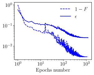
Figure 4: Comparison of the infidelity $1-F$ and the prediction error $\epsilon$ against the number of learning epochs during the learning process of the IM for the XXX model. The XXX-model is defined by a Floquet operator in Eq. (15) with $J=J^{\prime}=0.1$. The initial state of the system and environment is $\ket{\uparrow}\bra{\uparrow}\otimes\rho_{\downarrow}$, the dataset size is $N=5\cdot 10^{6}$. Both metrics show that the IM can be reconstructed faithfully.

During the learning process the infidelity quickly drops below $10^{-2}$ for $N=5\cdot 10^{6}$ samples. This means that the relative error of the IM reconstruction is small for machine learning approaches. However, in our case the IM is a large tensor with $2^{4t}$ elements, and its norm strongly depends on the nature of the environment. Specifically, its Frobenius norm satisfies an inequality $1\leq\sqrt{\langle\mathcal{J}_{\rm r}|\mathcal{J}_{\rm r}\rangle}\leq 2^{t}$, where the lower bound is saturated when IM is a fully depolarising quantum channel, and the upper bound is saturated for an IM which is seen as a unitary quantum channel. Thus, Frobenius norm of $\ket{\mathcal{J}_{\rm r}}$ could be exponentially large in general. Since an expectation value of an impurity observable is proportional to $\ket{\mathcal{J}_{\rm r}}$ without the normalization factor, its absolute error could be as large as $\mathcal{O}\left(\sqrt{\left(1-\sqrt{F}\right)\langle\mathcal{J}_{\rm r}|\mathcal{J}_{\rm r}\rangle}\right)$. Therefore, even a small relative error could in principle significantly affect the prediction accuracy for impurity observables. However, we find that this is not the case: the prediction error $\epsilon$ reaches values of $\epsilon\approx 0.025$ for $N=5\cdot 10^{6}$ at the end of the learning protocol, indicating that the impurity dynamics is reproduced faithfully. Both metrics become stationary after around $10^{3}$ epochs, indicating that the learning process is converged.

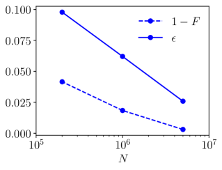
Figure 5: Comparison of the infidelity $1-F$ and the prediction error $\epsilon$ at the final point of the learning process against the dataset size for the XXX model. Both metrics show that quality of IM reconstruction and prediction accuracy systematically improve with increasing the dataset size.

The above results indicate that the reconstructed IM allows an accurate prediction of the dynamics of an impurity coupled to a single environment. Furthermore, the IMs learned in an experiment with a single environment has a broader applicability. In particular, it can be used to make predictions in quantum transport setups that involve multiple environments (leads), for arbitrary time-dependent impurity Hamiltonian.

We illustrate this by studying time evolution of an impurity coupled to left and right environments, which are chosen to be semi-infinite XX or XXX chains, with initial states $\rho^{L(R)}$ and corresponding IMs $\mathcal{J}^{L(R)}$. We choose the impurity to consist of two spins coupled by a generic XYZ interaction; it is then convenient to think of the system as a spin chain, with the impurity sites at $i=0,1$. The quantum channel applied to the impurity over one time step is given by,

$$W(J_{x},J_{y},J_{z})[\cdot]=U_{\rm imp}(J_{x},J_{y},J_{z})\cdot U_{\rm imp}^{\dagger}(J_{x},J_{y},J_{z}),$$

$$U_{\rm imp}(J_{x},J_{y},J_{z})=e^{-i\left(J_{x}X_{0}X_{1}+J_{y}Y_{0}Y_{1}+J_{z}Z_{0}Z_{1}\right)},$$ (19)

where $\cdot$ denotes the density matrix of impurity. Note that the choice of parameters $J_{x}=J_{y}=J$ and $J_{z}=J^{\prime}$ corresponds to a homogeneous infinite chain.

We start by considering a quantum transport setup where impurity is initialized in an out-of-equilibrium state and is coupled to the leads at time $t=0$. For this numerical experiment, the initial density matrices of the left and right environments are chosen to be infinite-temperature states. We set the initial density matrix of the impurity to the following pure state

$$\rho^{I}(0)=\ket{\uparrow}\bra{\uparrow}\otimes\ket{\uparrow}\bra{\uparrow},$$ (20)

and $J=J^{\prime}=0.1$ for both environments. In Fig. 6 we compare the dynamics of the diagonal elements of $\rho^{I}(t)$ computed using the first-principles IM with the dynamics computed with the IM reconstructed using a dataset of size $N=5\cdot 10^{6}$. As impurity’s quantum channel parameters we choose $J_{x}=J_{y}=J_{z}=0.1$ corresponding to the integrable homogeneous chain and $J_{x}=0.2$, $J_{y}=J_{z}=0.1$ corresponding to a non-integrable chain with an impurity. It is evident that the time evolution obtained using the reconstructed IMs closely follows that obtained from first-principles IMs. This is a highly nontrivial observation, since two environments interact with each other via the impurity and the physics of this interaction is correctly captured by the IMs reconstructed from a numerical experiment with a single environment.

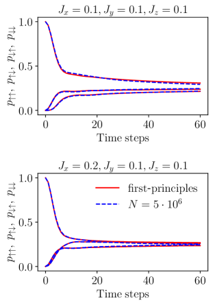
Figure 6: Dynamics of diagonal elements of the impurity’s density matrix, $p_{\uparrow\uparrow}=\bra{\uparrow}\otimes\bra{\uparrow}\rho^{I}\ket{\uparrow}\otimes\ket{\uparrow}$, $p_{\uparrow\downarrow}=\bra{\uparrow}\otimes\bra{\downarrow}\rho^{I}\ket{\uparrow}\otimes\ket{\downarrow}$, $p_{\downarrow\uparrow}=\bra{\downarrow}\otimes\bra{\uparrow}\rho^{I}\ket{\downarrow}\otimes\ket{\uparrow}$, $p_{\downarrow\downarrow}=\bra{\downarrow}\otimes\bra{\downarrow}\rho^{I}\ket{\downarrow}\otimes\ket{\downarrow}$, for the transport setup with environments being XXX semi-infinite spin chains, defined in Eq. (15), with $J=J^{\prime}=0.1$. Impurity evolution is given by Eq. (19). The solid red curves represent results obtained using first-principles IMs, while the dashed blue curves are obtained from reconstructed IMs. The dataset size used to reconstruct IMs is $N=5\cdot 10^{6}$.

Next, we consider relaxation of an initial domain wall configuration in a homogeneous XXX spin chain, corresponding to the choice of parameters, $J_{x}=J_{y}=J$ and $J_{z}=J^{\prime}=J$. In this case, the total $Z$-projection of spin is conserved. The initial state of the left environment is chosen to be polarized down $\rho^{L}=\rho_{\downarrow}$ and the initial state of the right environment to be polarized up $\rho^{R}=\rho_{\uparrow}$, while an impurity is initialized in a state

$$\rho^{I}(0)=\ket{\downarrow}\bra{\downarrow}\otimes\ket{\uparrow}\bra{\uparrow},$$ (21)

corresponding to a domain wall at $x=1/2$. Similar setups have been recently probed experimentally [51, 52]. Setting $J=J^{\prime}=0.1$ and $J=J^{\prime}=0.2$, we computed the instantaneous current through the domain wall by Eq. (9) using first-principles IM and the reconstructed ones. The comparison of these two computations for different dataset sizes $N$ is provided in Fig. 7. One observes that the current dynamics prediction based on the reconstructed IMs improves with increasing dataset size. While for short times the agreement is near perfect, the results based on the reconstructed IMs exhibit slight deviation from the reference ones even for the largest dataset size, $N=5\cdot 10^{6}$.

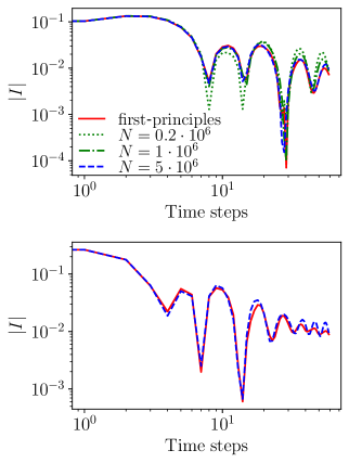
Figure 7: Instantaneous current flowing through the impurity coupled with two XXX environments Eq. (15) for $J=J^{\prime}=0.1$ (top panel) and for $J=J^{\prime}=0.2$ (bottom panel). Solid red curves are obtained by using first-principles IMs, dashed curves are obtained by using the reconstructed IMs from datasets of different size.

Finally, we demonstrate that reconstructed IMs correctly capture long-time non-Markovian effects, as well as a response to an external control signal. To that end, we consider a two-site impurity in an initial state $\rho^{I}(0)=\ket{\downarrow}\bra{\downarrow}\otimes\ket{\downarrow}\bra{\downarrow}$ coupled with two XX semi-infinite chains with $J=0.1,J^{\prime}=0$ and initial states $\rho^{L}=\rho_{\downarrow}$, $\rho^{R}=\rho_{\uparrow}$. The time-dependent impurity channel $W^{(\tau)}$ is chosen as follows

$$W^{(\tau)}[\cdot]=\begin{cases}U_{\rm imp}(J,J,J^{\prime})\cdot U^{\dagger}_{\rm imp}(J,J,J^{\prime}),\ \tau<20,\\ \mathcal{D}[\cdot],\ \tau=20,\\ {\rm Id}[\cdot],\ \tau>20,\end{cases}$$ (22)

where $\mathcal{D}$ is an amplitude damping channel turning any impurity’s state into $\ket{\downarrow}\bra{\downarrow}\otimes\ket{\downarrow}\bra{\downarrow}$, and ${\rm Id}$ is the identity channel. Note that the impurity dynamics in this case can be calculated exactly, since this model is non-interacting. Impurity dynamics described by Eq. (22) can be described as follows: first, at times $t<20$, there is a current flowing from right to left part of the system, and density on the impurity is increasing towards a steady-state value of $n_{0}=1/2$. Further, at time $t=20$, the impurity is reset to a state without particles, and left and right sites of the impurity are decoupled, such that each site is now coupled only to one environment. During subsequent evolution, we expect the occupation number of the left impurity site, $n(\tau)$ to exhibit a peak due to the backflow of particles which were transferred from the right environment to the left one during time $t<20$, before settling to a value of $n=0$ at long times. Such a peak is a reflection of non-Markovianity of system’s dynamics. In Fig. 8 we compare dynamics of the particles number on the left impurity qubit ${n}(\tau)$ computed exactly, with the first-principles IM and with the reconstructed IM. The reconstructed IM follows the exact results closely, in particular reproducing the peak around the time $t=25$. We provide additional numerical results for other environments and impurity time evolution in Appendix E.

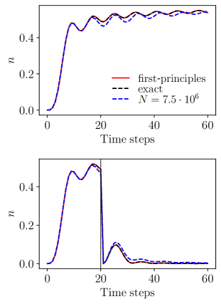
Figure 8: Dynamics of the occupation number on the impurity’s left qubit under a control signal in Eq. (22) (bottom panel) and without time dependent control (top panel). Solid red curves are computed by using the first-principles IM, dashed black curves are computed exactly using the free fermion representation, and dashed blue curves are computed with use of the reconstructed IM. The vertical black line in the bottom panel highlights the moment when particles are removed from the impurity and two sites of the impurity are decoupled.

V Discussion and Outlook

In summary, in this paper we investigated a hybrid algorithm for reconstructing IMs of large many-body environments. Using several examples, where measurement data were mimicked using a classical computation, we found that the IMs for long-time evolution could be efficiently learned from a relatively limited number of measurements. The efficiency of this approach relies on the moderate scaling of IMs temporal entanglement with evolution time, which allows for an MPS representation. Our work builds on, and complements previous works, Refs. [36, 37], where a process tensor was reconstructed from experimental data, for a few time steps.

The MPS representation of an environment’s IM allows for efficient classical computations of arbitrary dynamics of a small quantum system interacting with that environment. In particular, as an application of the proposed algorithm, we considered several quantum transport setups in 1d systems, including an impurity coupled to XX and XXX spin half-chain environments, as well as a quantum quench starting from a domain wall state. We demonstrated that an IM learned from an experiment with a single environment allowed us to accurately model setups with multiple leads. We envision this to be useful, e.g. in cases where a quantum processor has enough degrees of freedom to simulate a single environment, but is not suitable for directly modeling multiple leads.

Among the most promising applications of the proposed approach is learning the structure of IMs for many-body environments where no efficient classical algorithm is currently available, but there are physical arguments suggesting the area-law scaling of the temporal entanglement. One class of such systems are non-integrable systems with long-lived quasiparticles, e.g. interacting 2d Fermi liquids. Furthermore, IM learning may shed light on the issue of TE scaling in thermalizing many-body systems. On the one hand, intuitively one may expect that a large thermalizing systems act as baths with a finite memory time (thermalization time), leading to an area-law TE; on the other hand, recent studies of temporal entanglement in quantum circuits [17, 53], in particular in proximity to dual-unitary points and in random circuits, point to a volume-law scaling. It would be interesting to apply the approach of this paper to learn IMs for a broader class of thermalizing environments realized using quantum processors. The ability to reconstruct the IM in an MPS form would signal area-law TE. While we generally expect the learning procedure to fail for IMs with volume-law TE, it is an interesting open question whether in such cases there exists an area-law temporally-entangled IM which approximates the environment effect for certain restricted classes of impurity’s dynamics.

VI Acknowledgements

The computations were performed at University of Geneva using Baobab HPC service. We thank Alessio Lerose, Julian Thoenniss, and Ilya Vilkoviskiy for helpful discussions and collaboration on related topics, and Juan Carrasquilla for insightful discussions. This work was partially supported by the European Research Council (ERC) under the European Union’s Horizon 2020 research and innovation program (grant agreement No. 864597) and by the Swiss National Science Foundation.

Appendix A Vectorization

To introduce the vectorized operators extensively used in the main text, such as in Eq. (1), we need to define a basis of operators and enumerate its elements using a single index. For this purpose, we employ a basis of matrix units, which, for a single-qubit case, reads

$$e_{0}=\ket{0}\bra{0},\ e_{1}=\ket{1}\bra{0},\ e_{2}=\ket{0}\bra{1},\ e_{3}=\ket{1}\bra{1}.$$ (23)

Then, any operator can be vectorized as follows

$$O_{k}={\rm Tr}\left({e_{k}O}\right),$$ (24)

where $O$ is an arbitrary one-qubit operator. Also, any $m$-subsystem density matrix can be vectorized as follows

$$\rho_{k_{1}\dots k_{m}}={\rm Tr}\left(\left[\bigotimes_{i=1}^{m}e_{k_{i}}\right]\rho\right).$$ (25)

Appendix B Information complete measurements

To extract information from the Choi state of an IM, we perform a symmetric, informationally complete (SIC) positive operator-valued (POVM) measurement of each qubit of the Choi state. A POVM measurement is the most general measurement allowed by quantum theory. It is defined by a set of positive semi-definite Hermitian matrices $\{M^{\alpha}\}_{\alpha=0}^{3}$, where each matrix corresponds to a particular measurement result, and these matrices sum to the identity matrix, i.e. $\sum_{\alpha=0}^{3}M^{\alpha}=\mathds{1}$. The probability of getting a particular measurement result is given by the Born rule $p[\alpha]={\rm Tr}(\rho M^{\alpha})$, where $\rho$ is a density matrix. In the vectorized form it reads $p[\alpha]=M^{\alpha}_{i}\rho_{i}$, where $i$ runs over all entries of a POVM element and a density matrix. Information completeness means that the measured state can be exactly reconstructed from measurement results in the limit of an infinite number of measurements or that the matrix $M^{\alpha}_{i}$ is invertible. Symmetry means that the number of POVM elements is the minimal possible guaranteeing information completeness ($4$ for a qubit) and that the POVM is highly symmetric in some sense [54]. We choose a particular example of SIC-POVM that is defined by a set of vectorized operators enumerated by $\alpha\in\{0,1,2,3\}$

$$M^{\alpha}_{i}=\frac{1}{4}\left(\mathds{1}_{i}+s^{\alpha}_{k}\sigma^{k}_{i}\right),$$ (26)

where index $i$ runs over all entries of the vectorized POVM element, $\sigma^{k}_{i}$ are vectorized Pauli matrices enumerated by $k$ and

$$s^{\alpha}_{k}=\begin{bmatrix}0&0&1\\ \frac{2\sqrt{2}}{2}&0&-\frac{1}{3}\\ -\frac{\sqrt{2}}{3}&\sqrt{\frac{2}{3}}&-\frac{1}{3}\\ -\frac{\sqrt{2}}{3}&-\sqrt{\frac{2}{3}}&-\frac{1}{3}\end{bmatrix},$$ (27)

where $\alpha$ enumerates the rows and $k$ enumerates the columns. Note, that the rows of the matrix Eq. (27) are the coordinates of the vertices of a tetrahedron, which justifies the symmetry of this POVM. Since each qubit measurement ends up as a particular value of $\alpha$, the measurement result of the entire state is a string with numbers from a set $\{0,1,2,3\}$. A set of these strings form a dataset that is used for further IM recovery.

Appendix C Optimization algorithm

The central computational problem of the present algorithm is the following constrained optimization problem

$$\underset{\Theta,\rho}{\rm maximize}\quad\mathcal{L}(\mathbf{X},\Theta,\rho)$$

$${\rm subject\ to}\quad\Theta\in{\rm CPTP},\ {\rm Tr}(\rho)=1,\ \rho\geq 0.$$ (28)

First, we note that any density matrix can be represented as follows $\rho=\phi[1]$, where $\phi$ is a CPTP map that maps a $1\times 1$ density matrix (a scalar $1$) to $\rho$. This brings us to an optimization problem with only CPTP constraints

$$\underset{\Theta,\phi}{\rm maximize}\quad\mathcal{L}^{{}^{\prime}}(\mathbf{X},\Theta,\phi)$$

$${\rm subject\ to}\quad\Theta,\phi\in{\rm CPTP}.$$ (29)

Note that due to the Stinespring dilation, one can parametrize both CPTP maps taking part in the optimization problem as follows

$$\Theta[\cdot] ={\rm Tr}_{A}\left(V\cdot V^{\dagger}\right),$$

$$\phi[\cdot] ={\rm Tr}_{A}\left(v\cdot v^{\dagger}\right),$$ (30)

where ${\rm Tr}_{A}$ is a partial trace over an $r$-dimensional auxiliary space, $V$ is an isometric matrix of size $rn\times n$, $v$ is an isometric matrix of size $rn\times 1$, $n$ is a square root of the ansatz bond dimension. Note, that to parametrize an arbitrary CPTP map one needs $r\geq n^{2}$ for $V$ and $r\geq n$ for $v$, but taking $r$ smaller we can regularize the learning procedure by restricting the amount of dissipation introduced by an ansatz. We use $r$ as another hyperparameter and call it a local Choi rank. Using the parametrization above, we turn the optimization problem to the following one

$$\underset{V,v}{\rm maximize}\quad\mathcal{L}^{{}^{\prime\prime}}(\mathbf{X},V,v)$$

$${\rm subject\ to}\quad V\in{\rm St}(nr,n),\ v\in{\rm St}(rn,1),$$ (31)

where ${\rm St}$ denotes a set of all isometric matrices of a given size also called a Stiefel manifold. Since this set is a differentiable manifold, one can solve the given problem using Riemannian optimization techniques, i.e., a variation of gradient descent that operates within a differentiable manifold. Here we use so-called Riemannian ADAM optimizer which is the Riemannian generalization of the ADAM optimizer popular in the field of deep learning.

Appendix D Details on learning experiments

In our numerical experiments, we considered $8$ different first-principles IMs that we mark as follows: (i) XXX, $J=0.1$, $\rho_{\uparrow}$; (ii) XXX, $J=0.1$, $\rho_{\downarrow}$; (iii) XXX, $J=0.1$, $\rho_{\infty}$; (iv) XXX, $J=0.2$, $\rho_{\uparrow}$; (v) XXX, $J=0.2$, $\rho_{\downarrow}$; (vi) XX, $J=0.1$, $\rho_{\uparrow}$; (vii) XX, $J=0.1$, $\rho_{\downarrow}$; (viii) XX, $J=0.1$, $\rho_{\infty}$. Here XXX or XX classifies a model type, $J$ is a physical time spent per discrete time step, $\rho_{\uparrow}$, $\rho_{\downarrow}$, $\rho_{\infty}$ are initial states of an environment. All IMs have $60$ discrete time steps and maximum bond dimension of $\chi=256$.

For each IM we generated datasets of measurement strings: $3$ datasets of different size for IMs (i) and (ii), and one dataset per IM for the rest. Dataset sizes are given in the Table 1. Some of the datasets were collected using coarse graining: half of each of those datasets was collected with passing a Bell state’s part through $10$ time steps and another half was collected without coarse graining. Datasets with coarse graining are emphasized in the Table 1.

Each dataset was used to reconstruct an IM using the developed learning algorithm. The bond dimension and the local Choi rank (see Appendix C for a reference on what we call a local Choi rank) of an ansatz for each case are given in Table 1. For all learning experiments we set batch size to $5000$ measurement strings, initial learning rate to $0.25$. The number of learning epochs and the final learning rate were different for XXX and XX cases. Their values are given in the Table 1. The learning rate decayed exponentially from the initial value to the final value during the training. In all experiments we used Riemannian ADAM optimizer on the Stiefel manifold with parameters $\beta_{1}=0.9$, $\beta_{2}=0.999$, $\epsilon=10^{-8}$.

Table 1: Some parameters of learning experiments that vary from one IM to another.

	XXX, $J=0.1$, $\rho_{\uparrow}$	XXX, $J=0.1$, $\rho_{\downarrow}$	XXX, $J=0.1$, $\rho_{\infty}$	XXX, $J=0.2$, $\rho_{\uparrow}$	XXX, $J=0.2$, $\rho_{\downarrow}$	XX, $J=0.1$, $\rho_{\uparrow}$	XX, $J=0.1$, $\rho_{\downarrow}$	XX, $J=0.1$, $\rho_{\infty}$
Dataset size	$0.2\cdot 10^{6}$ $1\cdot 10^{6}$ $5\cdot 10^{6}$	$0.2\cdot 10^{6}$ $1\cdot 10^{6}$ $5\cdot 10^{6}$	$5\cdot 10^{6}$	$5\cdot 10^{6}$	$5\cdot 10^{6}$	$7.5\cdot 10^{6}$	$7.5\cdot 10^{6}$	$7.5\cdot 10^{6}$
Ansatz local Choi rank	100	100	100	100	100	16	16	16
Coarse graining	Yes	Yes	Yes	Yes	Yes	No	No	No
Training epochs number	1200	1200	1200	1200	1200	2400	2400	2400
Final learning rate	$10^{-5}$	$10^{-5}$	$10^{-5}$	$10^{-5}$	$10^{-5}$	$10^{-3}$	$10^{-3}$	$10^{-3}$

Appendix E More numerical results

In this appendix we give additional numerical results. Each additional numerical experiment is classified by the type of left and right environments (XX or XXX), initial states of left and right environment ($\rho^{L}$ and ${\rho^{R}}$), constants $J_{x}$, $J_{y}$ and $J_{z}$ defining a quantum channel acting on the impurity Eq. (19). Constants $J_{x}$, $J_{y}$ and $J_{z}$ are sampled uniformly from a cube $[-1,1]^{3}$ and rounded to two decimal places. For all the environments we set $J=0.1$. In Fig. 9 and Fig. 10 we provide a comparison of first-principles dynamics of diagonal elements of the impurity density matrix with the dynamics based on learned IMs.

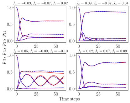
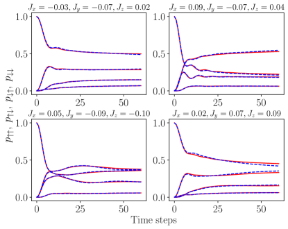
Figure 9: The comparison of the first-principles dynamics (solid lines) of the impurity density matrix diagonal elements, that are given by $p_{\uparrow\uparrow}=\bra{\uparrow}\otimes\bra{\uparrow}\rho^{I}\ket{\uparrow}\otimes\ket{\uparrow}$, $p_{\uparrow\downarrow}=\bra{\uparrow}\otimes\bra{\downarrow}\rho^{I}\ket{\uparrow}\otimes\ket{\downarrow}$, $p_{\downarrow\uparrow}=\bra{\downarrow}\otimes\bra{\uparrow}\rho^{I}\ket{\downarrow}\otimes\ket{\uparrow}$, $p_{\downarrow\downarrow}=\bra{\downarrow}\otimes\bra{\downarrow}\rho^{I}\ket{\downarrow}\otimes\ket{\downarrow}$, with the dynamics predicted using learned IMs (dashed lines). The left panel corresponds to XXX environments with initial states being $\rho^{L}=\rho_{\downarrow}$ and $\rho^{R}=\rho_{\uparrow}$, the right panel corresponds to XXX environments with initial states being $\rho^{L}=\rho_{\infty}$ and $\rho^{R}=\rho_{\uparrow}$. The size of datasets used to learn influence matrices is $N=5\cdot 10^{6}$. The initial state of the impurity is $\rho^{I}(0)=\ket{\uparrow}\bra{\uparrow}\otimes\ket{\uparrow}\bra{\uparrow}$.

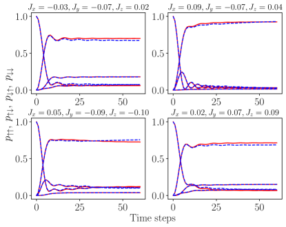
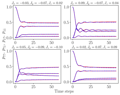
Figure 10: The comparison of the first-principles dynamics (solid lines) of the impurity density matrix diagonal elements, that are given by $p_{\uparrow\uparrow}=\bra{\uparrow}\otimes\bra{\uparrow}\rho^{I}\ket{\uparrow}\otimes\ket{\uparrow}$, $p_{\uparrow\downarrow}=\bra{\uparrow}\otimes\bra{\downarrow}\rho^{I}\ket{\uparrow}\otimes\ket{\downarrow}$, $p_{\downarrow\uparrow}=\bra{\downarrow}\otimes\bra{\uparrow}\rho^{I}\ket{\downarrow}\otimes\ket{\uparrow}$, $p_{\downarrow\downarrow}=\bra{\downarrow}\otimes\bra{\downarrow}\rho^{I}\ket{\downarrow}\otimes\ket{\downarrow}$, with the dynamics predicted using learned influence matrices (dashed lines). The left panel corresponds to XX environments with initial states being $\rho^{L}=\rho_{\downarrow}$ and $\rho^{R}=\rho_{\uparrow}$, the right panel corresponds to XX environments with initial states being $\rho^{L}=\rho_{\infty}$ and $\rho^{R}=\rho_{\uparrow}$. The size of datasets used to learn influence matrices is $N=7.5\cdot 10^{6}$. The initial state of the impurity is $\rho^{I}(0)=\ket{\uparrow}\bra{\uparrow}\otimes\ket{\uparrow}\bra{\uparrow}$.

References

- Preskill [2018] J. Preskill, Quantum Computing in the NISQ era and beyond, Quantum 2, 79 (2018).
- Altman et al. [2021] E. Altman, K. R. Brown, G. Carleo, L. D. Carr, E. Demler, C. Chin, B. DeMarco, S. E. Economou, M. A. Eriksson, K.-M. C. Fu, et al., Quantum simulators: Architectures and opportunities, PRX Quantum 2, 017003 (2021).
- Daley et al. [2022] A. J. Daley, I. Bloch, C. Kokail, S. Flannigan, N. Pearson, M. Troyer, and P. Zoller, Practical quantum advantage in quantum simulation, Nature 607, 667 (2022).
- Arute et al. [2019] F. Arute, K. Arya, R. Babbush, D. Bacon, J. C. Bardin, R. Barends, R. Biswas, S. Boixo, F. G. Brandao, D. A. Buell, et al., Quantum supremacy using a programmable superconducting processor, Nature 574, 505 (2019).
- Wu et al. [2021] Y. Wu, W.-S. Bao, S. Cao, F. Chen, M.-C. Chen, X. Chen, T.-H. Chung, H. Deng, Y. Du, D. Fan, M. Gong, C. Guo, C. Guo, S. Guo, L. Han, L. Hong, H.-L. Huang, Y.-H. Huo, L. Li, N. Li, S. Li, Y. Li, F. Liang, C. Lin, J. Lin, H. Qian, D. Qiao, H. Rong, H. Su, L. Sun, L. Wang, S. Wang, D. Wu, Y. Xu, K. Yan, W. Yang, Y. Yang, Y. Ye, J. Yin, C. Ying, J. Yu, C. Zha, C. Zhang, H. Zhang, K. Zhang, Y. Zhang, H. Zhao, Y. Zhao, L. Zhou, Q. Zhu, C.-Y. Lu, C.-Z. Peng, X. Zhu, and J.-W. Pan, Strong quantum computational advantage using a superconducting quantum processor, Phys. Rev. Lett. 127, 180501 (2021).
- Schreiber et al. [2015] M. Schreiber, S. S. Hodgman, P. Bordia, H. P. Lüschen, M. H. Fischer, R. Vosk, E. Altman, U. Schneider, and I. Bloch, Observation of many-body localization of interacting fermions in a quasirandom optical lattice, Science 349, 842 (2015).
- Langen et al. [2015] T. Langen, S. Erne, R. Geiger, B. Rauer, T. Schweigler, M. Kuhnert, W. Rohringer, I. E. Mazets, T. Gasenzer, and J. Schmiedmayer, Experimental observation of a generalized gibbs ensemble, Science 348, 207 (2015).
- Kaufman et al. [2016] A. M. Kaufman, M. E. Tai, A. Lukin, M. Rispoli, R. Schittko, P. M. Preiss, and M. Greiner, Quantum thermalization through entanglement in an isolated many-body system, Science 353, 794 (2016).
- Abanin et al. [2019] D. A. Abanin, E. Altman, I. Bloch, and M. Serbyn, Colloquium: Many-body localization, thermalization, and entanglement, Rev. Mod. Phys. 91, 021001 (2019).
- Schollwöck [2011] U. Schollwöck, The density-matrix renormalization group in the age of matrix product states, Annals of physics 326, 96 (2011).
- Cirac et al. [2021] J. I. Cirac, D. Perez-Garcia, N. Schuch, and F. Verstraete, Matrix product states and projected entangled pair states: Concepts, symmetries, theorems, Reviews of Modern Physics 93, 045003 (2021).
- Vidal [2004] G. Vidal, Efficient simulation of one-dimensional quantum many-body systems, Physical review letters 93, 040502 (2004).
- White and Feiguin [2004] S. R. White and A. E. Feiguin, Real-time evolution using the density matrix renormalization group, Physical review letters 93, 076401 (2004).
- Paeckel et al. [2019] S. Paeckel, T. Köhler, A. Swoboda, S. R. Manmana, U. Schollwöck, and C. Hubig, Time-evolution methods for matrix-product states, Annals of Physics 411, 167998 (2019).
- Bertini et al. [2021] B. Bertini, F. Heidrich-Meisner, C. Karrasch, T. Prosen, R. Steinigeweg, and M. Žnidarič, Finite-temperature transport in one-dimensional quantum lattice models, Rev. Mod. Phys. 93, 025003 (2021).
- Bañuls et al. [2009] M. C. Bañuls, M. B. Hastings, F. Verstraete, and J. I. Cirac, Matrix Product States for Dynamical Simulation of Infinite Chains, Physical Review Letters 102, 240603 (2009).
- Lerose et al. [2021a] A. Lerose, M. Sonner, and D. A. Abanin, Influence matrix approach to many-body Floquet dynamics, Physical Review X 11, 021040 (2021a).
- Sonner et al. [2021] M. Sonner, A. Lerose, and D. A. Abanin, Influence functional of many-body systems: Temporal entanglement and matrix-product state representation, Annals of Physics 435, 168677 (2021).
- Ye and Chan [2021] E. Ye and G. K.-L. Chan, Constructing tensor network influence functionals for general quantum dynamics, The Journal of Chemical Physics 155, 044104 (2021).
- Frías-Pérez and Bañuls [2022] M. Frías-Pérez and M. C. Bañuls, Light cone tensor network and time evolution, Physical Review B 106, 115117 (2022).
- Lerose et al. [2023] A. Lerose, M. Sonner, and D. A. Abanin, Overcoming the entanglement barrier in quantum many-body dynamics via space-time duality, Physical Review B 107, L060305 (2023).
- Lerose et al. [2021b] A. Lerose, M. Sonner, and D. A. Abanin, Scaling of temporal entanglement in proximity to integrability, Physical Review B 104, 035137 (2021b).
- Strathearn et al. [2018] A. Strathearn, P. Kirton, D. Kilda, J. Keeling, and B. W. Lovett, Efficient non-markovian quantum dynamics using time-evolving matrix product operators, Nature communications 9, 3322 (2018).
- Cygorek et al. [2022] M. Cygorek, M. Cosacchi, A. Vagov, V. M. Axt, B. W. Lovett, J. Keeling, and E. M. Gauger, Simulation of open quantum systems by automated compression of arbitrary environments, Nature Physics 18, 662 (2022).
- Fux et al. [2023] G. E. Fux, D. Kilda, B. W. Lovett, and J. Keeling, Tensor network simulation of chains of non-markovian open quantum systems, Physical Review Research 5, 033078 (2023).
- Vilkoviskiy and Abanin [2024] I. Vilkoviskiy and D. A. Abanin, Bound on approximating non-markovian dynamics by tensor networks in the time domain, Physical Review B 109, 205126 (2024).
- Thoenniss et al. [2023a] J. Thoenniss, M. Sonner, A. Lerose, and D. A. Abanin, Efficient method for quantum impurity problems out of equilibrium, Physical Review B 107, L201115 (2023a).
- Thoenniss et al. [2023b] J. Thoenniss, A. Lerose, and D. A. Abanin, Nonequilibrium quantum impurity problems via matrix-product states in the temporal domain, Physical Review B 107, 195101 (2023b).
- Ng et al. [2023] N. Ng, G. Park, A. J. Millis, G. K.-L. Chan, and D. R. Reichman, Real-time evolution of anderson impurity models via tensor network influence functionals, Physical Review B 107, 125103 (2023).
- De Franceschi et al. [2002] S. De Franceschi, R. Hanson, W. Van Der Wiel, J. Elzerman, J. Wijpkema, T. Fujisawa, . f. S. Tarucha, and L. Kouwenhoven, Out-of-equilibrium kondo effect in a mesoscopic device, Physical Review Letters 89, 156801 (2002).
- Pustilnik and Glazman [2004] M. Pustilnik and L. Glazman, Kondo effect in quantum dots, Journal of Physics: Condensed Matter 16, R513 (2004).
- Georges et al. [1996] A. Georges, G. Kotliar, W. Krauth, and M. J. Rozenberg, Dynamical mean-field theory of strongly correlated fermion systems and the limit of infinite dimensions, Rev. Mod. Phys. 68, 13 (1996).
- Kotliar et al. [2006] G. Kotliar, S. Y. Savrasov, K. Haule, V. S. Oudovenko, O. Parcollet, and C. A. Marianetti, Electronic structure calculations with dynamical mean-field theory, Rev. Mod. Phys. 78, 865 (2006).
- Pollock et al. [2018a] F. A. Pollock, C. Rodríguez-Rosario, T. Frauenheim, M. Paternostro, and K. Modi, Non-Markovian quantum processes: Complete framework and efficient characterization, Physical Review A 97, 012127 (2018a).
- Pollock et al. [2018b] F. A. Pollock, C. Rodríguez-Rosario, T. Frauenheim, M. Paternostro, and K. Modi, Operational markov condition for quantum processes, Physical review letters 120, 040405 (2018b).
- White et al. [2020] G. A. L. White, C. D. Hill, F. A. Pollock, L. C. L. Hollenberg, and K. Modi, Demonstration of non-markovian process characterisation and control on a quantum processor, Nature Communications 11 (2020).
- White et al. [2022] G. White, F. Pollock, L. Hollenberg, K. Modi, and C. Hill, Non-markovian quantum process tomography, PRX Quantum 3 (2022).
- Milz et al. [2018] S. Milz, F. A. Pollock, and K. Modi, Reconstructing non-markovian quantum dynamics with limited control, Physical Review A 98 (2018).
- Guo et al. [2020] C. Guo, K. Modi, and D. Poletti, Tensor-network-based machine learning of non-markovian quantum processes, Physical Review A 102 (2020).
- Cramer et al. [2010] M. Cramer, M. B. Plenio, S. T. Flammia, R. Somma, D. Gross, S. D. Bartlett, O. Landon-Cardinal, D. Poulin, and Y.-K. Liu, Efficient quantum state tomography, Nature Communications 1 (2010).
- Giudice et al. [2022] G. Giudice, G. Giudici, M. Sonner, J. Thoenniss, A. Lerose, D. A. Abanin, and L. Piroli, Temporal Entanglement, Quasiparticles, and the Role of Interactions, Physical Review Letters 128, 220401 (2022).
- Feynman and Vernon [2000] R. P. Feynman and F. L. Vernon, The Theory of a General Quantum System Interacting with a Linear Dissipative System, Annals of Physics 281, 547 (2000).
- Sonner et al. [2022] M. Sonner, A. Lerose, and D. A. Abanin, Characterizing many-body localization via exact disorder-averaged quantum noise, Physical Review B 105, L020203 (2022).
- Choi [1975] M.-D. Choi, Completely positive linear maps on complex matrices, Linear algebra and its applications 10, 285 (1975).
- Jamiołkowski [1972] A. Jamiołkowski, Linear transformations which preserve trace and positive semidefiniteness of operators, Reports on Mathematical Physics 3, 275 (1972).
- Luchnikov et al. [2021a] I. Luchnikov, A. Ryzhov, S. Filippov, and H. Ouerdane, QGOpt: Riemannian optimization for quantum technologies, SciPost Physics 10, 079 (2021a).
- Luchnikov et al. [2021b] I. A. Luchnikov, M. E. Krechetov, and S. N. Filippov, Riemannian geometry and automatic differentiation for optimization problems of quantum physics and quantum technologies, New Journal of Physics 23, 073006 (2021b), 2007.01287 .
- Ljubotina et al. [2019] M. Ljubotina, M. Žnidarič, and T. Prosen, Kardar-parisi-zhang physics in the quantum heisenberg magnet, Physical review letters 122, 210602 (2019).
- Ferris and Vidal [2012] A. J. Ferris and G. Vidal, Perfect sampling with unitary tensor networks, Physical Review B 85, 165146 (2012).
- Chertkov et al. [2022] A. Chertkov, G. Ryzhakov, G. Novikov, and I. Oseledets, Optimization of functions given in the tensor train format, arXiv preprint arXiv:2209.14808 (2022).
- Wei et al. [2022] D. Wei, A. Rubio-Abadal, B. Ye, F. Machado, J. Kemp, K. Srakaew, S. Hollerith, J. Rui, S. Gopalakrishnan, N. Y. Yao, et al., Quantum gas microscopy of kardar-parisi-zhang superdiffusion, Science 376, 716 (2022).
- Rosenberg et al. [2024] E. Rosenberg, T. Andersen, R. Samajdar, A. Petukhov, J. Hoke, D. Abanin, A. Bengtsson, I. Drozdov, C. Erickson, P. Klimov, et al., Dynamics of magnetization at infinite temperature in a heisenberg spin chain, Science 384, 48 (2024).
- Foligno et al. [2023] A. Foligno, T. Zhou, and B. Bertini, Temporal entanglement in chaotic quantum circuits, Phys. Rev. X 13, 041008 (2023).
- Renes et al. [2004] J. M. Renes, R. Blume-Kohout, A. J. Scott, and C. M. Caves, Symmetric informationally complete quantum measurements, Journal of Mathematical Physics 45, 2171 (2004).