Using Speech Foundational Models in Loss Functions for Hearing Aid Speech Enhancement

Abstract

Machine learning techniques are an active area of research for speech enhancement for hearing aids, with one particular focus on improving the intelligibility of a noisy speech signal. Recent work has shown that feature encodings from self-supervised speech representation models can effectively capture speech intelligibility. In this work, it is shown that the distance between self-supervised speech representations of clean and noisy speech correlates more strongly with human intelligibility ratings than other signal-based metrics. Experiments show that training a speech enhancement model using this distance as part of a loss function improves the performance over using an SNR-based loss function, demonstrated by an increase in HASPI, STOI, PESQ and SI-SNR scores. This method takes inference of a high parameter count model only at training time, meaning the speech enhancement model can remain smaller, as is required for hearing aids.

I Introduction

Hearing impairment is a widespread problem worldwide [1] and especially in countries with ageing populations [2, 3]. There is an emerging interest in the development of hearing aid systems which incorporate neural network components [4, 5, 6, 7, 8, 9]. The particular focus of this development has been on increasing the intelligibility of speech in the processed input audio. A core challenge in this area is that neural hearing aid models must be computationally efficient to fit within hardware constraints. Standard loss functions used to train neural network-based hearing aid systems operate at a signal level, e.g., based on signal-to-noise ratio (SNR), scale-invariant signal-to-noise ratio (SI-SNR), or short-term objective intelligibility (STOI) [10, 11, 12]. However, recent work has shown that representations sourced from large speech foundational models (i.e., with high parameter count), such as Whisper [13] or WavLM [14], are able to well capture information about the intelligibility of the signal [15, 16, 17]. Previous work has explored how the distances between the self-supervised speech representation (SSSR) representations of clean speech and noisy speech correlate with speech quality metrics and how they can be used in loss functions [18] for single-channel noise reduction. However, the correlation with speech intelligibility metrics and application of SSSR based loss functions for hearing aid systems have not yet been well explored in the existing literature.

This paper investigates how distances between WavLM representations correlate with speech intelligibility (SI) and speech quality (SQ) metrics like the hearing aid speech perception index (HASPI) [19], STOI [12], perceptual evaluation of speech quality (PESQ) [20], and others, as well with real-world human speech intelligibility (HSI) ratings from listening tests, released as part of the 2^nd Clarity Prediction Challenge (CPC2) [21]. Further, the distances of the WavLM representations are evaluated for their usefulness as loss functions to train the denoising component of a neural hearing aid system. The proposed method shows an increase in terms of perceptually motivated enhancement metrics versus a traditional baseline [22], while maintaining the strict model parameter count, speed and memory consumption constraints typical of a hearing aid system. This is achieved by taking inference of the much larger WavLM model only during model training.

The structure of the paper is as follows. Section II introduces the use of WavLM in this work and provides some background of the prior work which uses SSSRs for speech enhancement. Section III defines a distance measure using the WavLM representations of signals, and investigates how this correlates with human intelligibility labels and perception-based metrics. Section IV describes the system which is subsequently used for the signal enhancement experiments in Section V, using the WavLM-based distance metric as a loss function. Results are presented in Section VI and Section VII concludes the paper.

II Self-Supervised Speech Representations for Speech Enhancement

SSSR such as wav2vec [23] and HuBERT [24] were initially designed and evaluated as front-end feature extractors for down-stream automatic speech recognition (ASR) tasks. More recently, WavLM was developed to support a broader set of speech processing tasks, including, e.g., speaker verification, or speaker diarization, which it achieves by not only learning masked speech prediction, but also by learning speech denoising during training [14].

Recent work has shown that WavLM and other SSSRs are powerful feature representations for quality [25] and intelligibility prediction [15]. Furthermore, the ability of SSSR-derived representations to encode quality and intelligibility-related information has been exploited in loss functions for the training of speech enhancement systems [18, 26], showing improved performance in comparison to traditional loss functions for speech enhancement.

Figure 1: Representations extracted from WavLM model stages.

WavLM is a neural network with two distinct stages as shown in Figure 1: a convolutional neural network (CNN) based encoder $\mathcal{W}_{\mathrm{FE}}$ and a Transformer [27] based output stage $\mathcal{W}_{\mathrm{OL}}$. The input to the encoder $\mathcal{W}_{\mathrm{FE}}$ is a time-domain signal $s$ and its output representation $\mathbf{S}_{\mathrm{FE}}$ has a dimension $F_{\mathrm{FE}}\times T$ with encoder output feature dimension $F_{\mathrm{FE}}=512$ for WavLM [14] and $T$ representing the variable number of frames depending on the length of the input audio $s$. $\mathbf{S}_{\mathrm{FE}}$ is the input to the Transformer-based WavLM decoder stage $\mathcal{W}_{\mathrm{OL}}$ which returns a final output representation $\mathbf{S}_{\mathrm{OL}}$ with dimensions $F_{\mathrm{OL}}\times T$. For WavLM the output layer feature dimension is $F_{\mathrm{OL}}=768$ [14]. Based on findings from previous work [18, 26], only the encoder representation $\mathbf{S}_{\mathrm{FE}}$ is used in the following. In this work, the WavLM Base model trained on the Librispeech $960$ hour dataset [28] is used, which has $94.7$ million parameters.

III WavLM Representation Distances

Initially, the distance between WavLM encoder representations of clean and enhanced speech signals is explored, with a loss function defined as

$$\mathcal{L}_{\mathrm{WLM}}\left(s,\hat{s}\right)=\frac{1}{TF_{\mathrm{FE}}}\sum^{T}_{t=1}\sum^{F_{\mathrm{FE}}}_{f=1}\left(\mathbf{S}_{\mathrm{FE}}[t,f]-\mathbf{\hat{S}}_{\mathrm{FE}}[t,f]\right)^{2},$$ (1)

where $\mathbf{S}_{\mathrm{FE}}=\mathcal{W}_{\mathrm{FE}}(s)$ and $\mathbf{\hat{S}}_{\mathrm{FE}}=\mathcal{W}_{\mathrm{FE}}(\hat{s})$ are the representations of the target and estimated signal, respectively. Please note that frame (time) index $t$ and feature index $f$ are omitted for brevity at most places in this paper.

This distance measure is compared with the signal-to-noise ratio (SNR) based loss function

$$\mathcal{L}_{\mathrm{SNR}}\left(s,\hat{s}\right)=-10\log_{10}\left(\frac{\|s\|^{2}}{\|s-\hat{s}\|^{2}+\tau\|s\|^{2}}\right),$$ (2)

which is commonly used for training the speech enhancement component of hearing aid systems, with $\tau=10^{-\mathrm{SNR}_{\mathrm{max}}/10}=0.001$ (where $\mathrm{SNR}_{\mathrm{max}}=30\text{dB}$) to prevent sufficiently denoised signals from dominating the training, as described in [29].

In the following, an analysis of how $\mathcal{L}_{\mathrm{SNR}}$ and $\mathcal{L}_{\mathrm{WLM}}$ correlate with human intelligibility labels, as well as other perception-based metrics will be conducted.

III-A The $2^{nd}$ Clarity Prediction Challenge (CPC2) Dataset

The CPC2 dataset is used to investigate the relationship between $\mathcal{L}_{\mathrm{WLM}}$ in (1) and $\mathcal{L}_{\mathrm{SNR}}$ in (2), and existing speech metrics and HSI labels. The task of CPC2 is to predict the intelligibility of a signal for listeners with hearing impairment.

The main signal assessed in CPC2 is the binaural output signal for left and right channels $\mathbf{\hat{s}}=[\hat{s}_{l},\hat{s}_{r}]=\mathcal{M}\left(\mathbf{x}\right)$, processed by a hearing aid (HA) $\mathcal{M}(\cdot)$ with $6$-channel noisy input signal $\mathbf{x}$ (for $3$ microphones in each (left and right) HA), containing a clean speech signal $\mathbf{s}$. The samples in the CPC2 dataset include an enhanced signal $\mathbf{\hat{s}}$, a target signal $\mathbf{s}$, and a HSI label, which is the proportion of words that a hearing-impaired listener was able to identify in $\mathbf{\hat{s}}$, as well as the audiogram of the respective listener [21]. The first training split is used, which contains $2779$ samples; the distribution of these samples is shown in Figure 2. For each sample in one of the training splits, $\mathcal{L}_{\mathrm{WLM}}$ and $\mathcal{L}_{\mathrm{SNR}}$ were calculated as in (1) and (2), respectively.

Figure 2: Distribution of human intelligibility labels in the CPC2 train set

III-B Correlation Analysis

Table I shows Pearson correlations between HSI labels, $-\mathcal{L}_{\mathrm{SNR}}$, $-\mathcal{L}_{\mathrm{WLM}}$, SI-SNR, HASPI, STOI, and PESQ, with scatter-plots visualising some of the correlations with human intelligibility labels in Figure 3. Negative values of $\mathcal{L}_{\mathrm{SNR}}$ and $\mathcal{L}_{\mathrm{WLM}}$ are used so that positive correlations are expected for all rows and columns. For each objective metric, values for each (left and right) channel are computed and the better score is taken.

Table I: Pearson correlations $r$ between HSI, losses under test and various speech metrics on the CPC2 dataset.

		Losses		SI-
Scores	HSI	-$\mathcal{L}_{\mathrm{WLM}}$	-$\mathcal{L}_{\mathrm{SNR}}$	SNR	HASPI	STOI	PESQ
HSI	1.00	0.59	-0.26	0.02	0.47	0.71	0.47
$-\mathcal{L}_{\mathrm{WLM}}$	0.59	1.00	-0.29	-0.08	0.43	0.74	0.70
$-\mathcal{L}_{\mathrm{SNR}}$	-0.26	-0.29	1.00	0.22	-0.16	-0.26	-0.31
SI-SNR	0.02	-0.08	0.22	1.00	0.08	0.19	-0.05
HASPI	0.47	0.43	-0.16	0.08	1.00	0.62	0.27
STOI	0.71	0.74	-0.26	0.19	0.62	1.00	0.64
PESQ	0.47	0.70	-0.31	-0.05	0.27	0.64	1.00

Figure 3: Correlations of $-\mathcal{L}_{\mathrm{SNR}}$, $-\mathcal{L}_{\mathrm{WLM}}$, HASPI and STOI with the human intelligibility labels for the CPC2 dataset.

One would expect that a higher SNR value (lower $\mathcal{L}_{\mathrm{SNR}}$) would indicate a higher intelligibility rating. Table I and the scatter plot in Figure 3 (top left) indicate the opposite; the signals with higher SNR did not necessarily indicate that they would have higher intelligibility. This is likely to be because the signals in the CPC2 dataset were not originally optimised with an SNR loss and do not necessarily match the levels of the references.

In contrast, $\mathcal{L}_{\mathrm{WLM}}$ shows considerably stronger correlation with human intelligibility shown in Figure 3 (top right) and the other metrics compared with $\mathcal{L}_{\mathrm{SNR}}$. The particularly strong correlation of $\mathcal{L}_{\mathrm{WLM}}$ with PESQ and STOI in the CPC2 data is consistent with other datasets [18]. This strength speaks to the suitability of $\mathcal{L}_{\mathrm{WLM}}$ as a loss function to train the denoising component of a hearing aid system; training the denoising model to minimize this distance should by proxy improve the performance in terms of these metrics.

Additionally, despite being the only metric considered which takes into account the severity of a listener’s hearing loss i.e is specifically designed to predict intelligibility scores for hearing impaired people, HASPI shows a weaker correlation with human intelligibility labels when compared with $\mathcal{L}_{\mathrm{WLM}}$ and STOI and has a similar level of correlation compared to PESQ, which is not aimed at assessing intelligibility. This brings into question the usefulness of HASPI as a metric. Alternatively, it indicates that the severity of hearing loss does not actually factor massively into distribution of the human intelligibility labels, which is consistent with the findings in [15].

IV Hearing Aid System

The hearing aid enhancement system trained in this work is an MC-Conv-TasNet-based system [22], which performed best in the 1^st Clarity Enhancement Challenge (CEC1), consisting of two independently trained systems (one for each ear). Since modern hearing aids have multiple microphones, the system for each ear will take a multi-channel input, and the system for each ear will output a single channel.

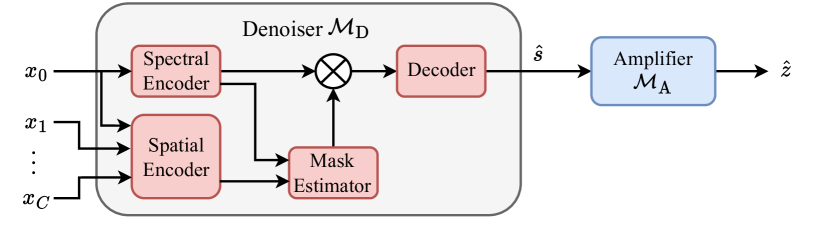
Figure 4: Workflow of the hearing aid system. For a $C$-channel signal $\mathbf{x}=\left[x_{0},\dots,x_{C}\right]$, a reference channel $x_{0}$ is input to the spectral encoder, while the spatial encoder takes all $C$ channels as input.

This is a two-stage system as illustrated in Figure 4, consisting of an MC-Conv-TasNet denoising block $\mathcal{M}_{\mathrm{D}}$ [30], followed by a finite-impulse response (FIR) filter block $\mathcal{M}_{\mathrm{A}}$ to amplify the signal according to a specific listener’s audiogram [31]. During training, the output of $\mathcal{M}_{\mathrm{A}}$ is passed into a differentiable hearing loss simulation before the loss function is applied.

The overall system consists of $4$ neural networks: a denoiser $\mathcal{M}_{\mathrm{D}}$ for each stereo channel, and an amplifier $\mathcal{M}_{\mathrm{A}}$ for each stereo channel. For each ear, the denoiser $\mathcal{M}_{\mathrm{D}}$ is trained first, then the parameters are frozen for training of the amplifier $\mathcal{M}_{\mathrm{A}}$.

IV-A Denoiser $\mathcal{M}_{D}$

The structure of MC-Conv-TasNet is given in Figure 4. This model consists of a spectral encoder, a spatial encoder, a mask estimation network, and a decoder. The spectral encoder is a $1$D convolutional network which takes a single reference channel from the multi-channel mixture and which has a kernel size $L$. The spatial encoder takes a multi-channel signal $\mathbf{x}$ as input and operates as a $2$D convolutional network over all channels; if $C$ denotes the number of microphone channels, the kernel size of the spatial encoder is $C\times L$ so that the number of frames of the spatial encoder is the same as the number of frames of the spectral encoder. The encoder outputs are concatenated as they are input to the mask estimator, which is a temporal convolutional network [32]. The mask is multiplied element-wise with the spectral encoder output to give the features of the estimated source. Finally, a decoder reconstructs a single-channel waveform as an estimate for the target.

The configuration of $\mathcal{M}_{D}$ is exactly as described in [22], where the spectral and spatial encoders use $256$ and $128$ filters, respectively, both with a frame length of $L=20$ samples. The $1\times 1$ bottleneck convolutional block uses $256$ channels and the convolutional blocks use $512$ channels. There are $6$ convolutional blocks, which have a kernel size of $3$ and dilation factors of $1,2,\dots,32$ and are repeated $4$ times. The input to $\mathcal{M}_{D}$ is the time domain multi-channel noisy signal $\mathbf{x}$ and the output is the denoised single channel audio $\hat{s}$.

IV-B Amplifier $\mathcal{M}_{A}$

The FIR filter amplification module [31], $\mathcal{M}_{A}$, is a simple, linear amplification model designed to compensate for hearing loss in each ear without introducing distortions and artefacts.

As with the denoiser, two independent amplification models are trained (one for each ear), taking the $22.05$kHz, single channel output of the denoising module $\mathcal{M}_{D}$. The result is upsampled to $44.1$kHz, clipped to the range $[-1,1]$, and fed into the differentiable hearing loss simulator $\mathcal{M}_{\mathrm{HL}}$. Upsampling is required as the hearing loss simulator used operates at $44.1$kHz.

V Experiment Setup

V-A Clarity Enhancement Challenge Datasets

Two datasets are used for training the system: the CEC1 dataset, for which the baseline system was designed, and the $2^{nd}$ Clarity Enhancement Challenge (CEC2) dataset, which is a more challenging dataset for the same task. Both of these datasets consist of a train set containing $6000$ samples, a validation set of $2500$ samples, and an evaluation set of $1500$ samples. Each sample is a $6$-channel, noisy, reverberant mixture $\mathbf{x}$, with a target, anechoic speech signal $\mathbf{s}=\left[s_{\mathrm{l}},s_{\mathrm{r}}\right]$ for each ear (left and right).

For CEC1, there is only one interfering source in the noisy mixture. In half of the samples, this is a second speech signal sourced from [33], and in the other half, the interfering signals are domestic noise sourced from [34]. For CEC2, there are $2$ or $3$ interfering sources in each noisy mixture, which could be competing speakers, music, or domestic noise. All data has a sampling frequency of $44.1$kHz.

V-B Training Setup

In this task, maintaining the signal level is important for the downstream amplification, which is required for hearing aid users. With this in mind, we propose a joint loss function

$$\mathcal{L}_{\mathrm{Joint}}\left(s,\hat{s}\right)=\mathcal{L}_{\mathrm{SNR}}\left(s,\hat{s}\right)+\mathcal{L}_{\mathrm{WLM}}\left(s,\hat{s}\right),$$ (3)

where $\mathcal{L}_{\mathrm{SNR}}$ is used to maintain the signal level of the reference.

In early experiments, it was found that $\mathcal{L}_{\mathrm{SNR}}$ and $\mathcal{L}_{\mathrm{WLM}}$ optimise with different learning rates, with $\mathcal{L}_{\mathrm{SNR}}$ preferring a greater learning rate. Two different training strategies are used, which vary the learning rate over the training process.

All modules were trained using the Adam optimiser [35]. The learning rate is initially set to $10^{-3}$, and gradient clipping is applied with a maximum L$2$-norm of $5$. Three training settings were used:

1. Baseline - The denoiser $\mathcal{M}_{D}$ was trained for $200$ epochs using the SNR loss function $\mathcal{L}_{\mathrm{SNR}}$ (2).

2. WavLM Encoder loss fine-tuning - $\mathcal{M}_{D}$ is trained for $100$ epochs using $\mathcal{L}_{\mathrm{SNR}}$ (2) followed by $100$ epochs of training using $\mathcal{L}_{\mathrm{Joint}}$ (3). During the fine-tuning stage, the learning rate is set to $10^{-4}$.

3. Joint Loss with learning rate scheduling - $\mathcal{M}_{D}$ is trained using the joint loss function $\mathcal{L}_{\mathrm{Joint}}$ (3) for $200$ epochs. A scheduled learning rate change inspired by [27] is used, with the learning rate linearly increasing for the first few training steps, and then with a learning rate decay over the remaining epochs.

Models for each (left and right) ear are trained separately; both sides take all $6$ channels of input (downsampled to $22.05$kHz), and the single corresponding left/right channel of the target audio is as the reference.

VI Results

Table II shows the evaluation metrics for the output of the denoiser $\mathcal{M}_{\mathrm{D}}$ for the baseline $\mathcal{L}_{\mathrm{SNR}}$ and the proposed $\mathcal{L}_{\mathrm{WLM}}$ for both the CEC1 and CEC2 test sets. On CEC1, the system trained with the proposed loss function using a scheduled learning rate shows a significant improvement on HASPI, STOI, PESQ and SI-SNR scores over the $\mathcal{L}_{\mathrm{SNR}}$ baseline, while the proposed fine-tuning approach performs similarly to the baseline.

On the more challenging CEC2 dataset, there is an improvement in HASPI and STOI for the proposed loss function using a scheduled learning rate, but the fine-tuning approach performs worse than the baseline. All systems give slightly lower PESQ scores on this dataset versus the noisy input; this is interesting given the strong correlation between these two metrics shown in Table I. It should, however, be noted that the main task of CEC is increasing intelligibility.

Table II: Performance of the denoiser $\mathcal{M}_{\mathrm{D}}$.

Dataset	Model	HASPI	STOI	PESQ	$\Delta$	$\Delta$
					SI-SNR	fwSNR
CEC1	$\mathcal{L}_{\mathrm{SNR}}$	0.90	0.76	1.19	7.92	3.72
	$\mathcal{L}_{\mathrm{WLM}}$, FT	0.90	0.76	1.20	8.03	3.42
	$\mathcal{L}_{\mathrm{WLM}}$, Sched.	0.91	0.78	1.23	8.45	1.65
CEC2	$\mathcal{L}_{\mathrm{SNR}}$	0.72	0.67	1.11	10.09	0.60
	$\mathcal{L}_{\mathrm{WLM}}$, FT	0.72	0.66	1.10	9.98	0.57
	$\mathcal{L}_{\mathrm{WLM}}$, Sched.	0.75	0.68	1.12	10.33	0.78

On CEC1, the HASPI improvement is only small, though the scores for all systems are very high for this metric. On CEC2, the improvement over the baseline is larger, and on this more challenging dataset, there is a perceptual improvement in these signals for listeners with hearing impairment.

VII Conclusion

In this work, it is shown that encoder representations obtained from WavLM can effectively capture the intelligibility of a speech signal. This is shown by implementing a simple distance function between representations of noisy and clean speech signals and correlating these distances with human intelligibility labels and perceptually motivated metrics for both intelligibility and quality. Further, this work evaluates the use of this distance in a loss function for training the denoising network of a hearing aid system. This new training setting shows improved performance over a system trained with a purely signal-based loss function, with improvements on HASPI, STOI, PESQ, and SI-SNR.

References

- [1] A. C. Davis and H. J. Hoffman, “Hearing loss: Rising Prevalence and Impact,” Bulletin of the World Health Organization, vol. 97, no. 10, pp. 646, 2019.
- [2] J. Rennies, S. Goetze, and J.-E. Appell, “Personalized Acoustic Interfaces for Human-Computer Interaction,” in Human-Centered Design of E-Health Technologies: Concepts, Methods and Applications, M. Ziefle and C.Röcker, Eds., chapter 8, pp. 180–207. IGI Global, 2011.
- [3] N. Park, “Population estimates for the UK, England and Wales, Scotland and Northern Ireland, provisional: mid-2019,” Hampshire: Office for National Statistics, 2020.
- [4] S. N. Graetzer, J. Barker, T. J. Cox, M. Akeroyd, J. F. Culling, G. Naylor, E. Porter, and R. Viveros Munoz, “Clarity-2021 challenges : Machine learning challenges for advancing hearing aid processing,” Proceedings of the Annual Conference of the International Speech Communication Association, INTERSPEECH, vol. 2, Sept. 2021.
- [5] S. Cornell, Z.-Q. Wang, Y. Masuyama, S. Watanabe, M. Pariente, and N. Ono, “Multi-channel target speaker extraction with refinement: The wavlab submission to the second clarity enhancement challenge,” in Proc. The 3rd Clarity Workshop on Machine Learning Challenges for Hearing Aids, Dec. 2022.
- [6] P. U. Diehl, Y. Singer, H. Zilly, U. Schönfeld, P. Meyer-Rachner, M. Berry, H. Sprekeler, E. Sprengel, A. Pudszuhn, and V. M. Hofmann, “Restoring speech intelligibility for hearing aid users with deep learning,” Scientific Reports, vol. 13, no. 2719, 2023.
- [7] C. Ouyang, K. Fei, H. Zhou, C. Lu, and L. Li, “A multi-stage low-latency enhancement system for hearing aids,” in Proc. ICASSP23, 2023, pp. 1–2.
- [8] H. Schröter, T. Rosenkranz, A.-N. Escalante-B, and A. Maier, “Low latency speech enhancement for hearing aids using deep filtering,” IEEE/ACM Transactions on Audio, Speech, and Language Processing, vol. 30, pp. 2716–2728, 2022.
- [9] I. Fedorov, M. Stamenovic, C. Jensen, L.-C. Yang, A. Mandell, Y. Gan, M. Mattina, and P. N. Whatmough, “TinyLSTMs: Efficient Neural Speech Enhancement for Hearing Aids,” in Proc. Interspeech 2020, 2020, pp. 4054–4058.
- [10] S. Braun and I. Tashev, “A consolidated view of loss functions for supervised deep learning-based speech enhancement,” in Proc. 44th Int. Conf. on Telecommunications and Signal Processing (TSP), 2021.
- [11] J. L. Roux, S. Wisdom, H. Erdogan, and J. R. Hershey, “Sdr – half-baked or well done?,” in ICASSP 2019 - 2019 IEEE International Conference on Acoustics, Speech and Signal Processing (ICASSP), 2019, pp. 626–630.
- [12] C. H. Taal, R. C. Hendriks, R. Heusdens, and J. Jensen, “An Algorithm for Intelligibility Prediction of Time–Frequency Weighted Noisy Speech,” IEEE Transactions on Audio, Speech, and Language Processing, vol. 19, no. 7, pp. 2125–2136, Sept. 2011.
- [13] A. Radford, J. W. Kim, T. Xu, G. Brockman, C. McLeavey, and I. Sutskever, “Robust Speech Recognition via Large-Scale Weak Supervision,” Dec. 2022.
- [14] S. Chen, C. Wang, Z. Chen, Y. Wu, S. Liu, Z. Chen, J. Li, N. Kanda, T. Yoshioka, X. Xiao, J. Wu, L. Zhou, S. Ren, Y. Qian, Y. Qian, J. Wu, M. Zeng, X. Yu, and F. Wei, “WavLM: Large-Scale Self-Supervised Pre-Training for Full Stack Speech Processing,” IEEE Journal of Selected Topics in Signal Processing, vol. 16, no. 6, pp. 1505–1518, Oct. 2022.
- [15] G. Close, T. Hain, and S. Goetze, “Non Intrusive Intelligibility Predictor for Hearing Impaired Individuals using Self Supervised Speech Representations,” in Proc. Workshop on Speech Foundation Models and their Performance Benchmarks (SPARKS), ASRU satelite workshop, Taipei, Taiwan, 2023.
- [16] S. Cuervo and R. Marxer, “Speech foundation models on intelligibility prediction for hearing-impaired listeners,” in Proc. ICASSP24, 2024.
- [17] R. Mogridge, G. Close, R. Sutherland, T. Hain, J. Barker, S. Goetze, and A. Ragni, “Non-intrusive speech intelligibility prediction for hearing-impaired users using intermediate asr features and human memory models,” in Proc. ICASSP 2024, 2024.
- [18] G. Close, W. Ravenscroft, T. Hain, and S. Goetze, “Perceive and predict: Self-supervised speech representation based loss functions for speech enhancement,” in Proc. ICASSP23, June 2023, pp. 1–5.
- [19] J. M. Kates and K. H. Arehart, “The hearing-aid speech perception index (haspi) version 2,” Speech Communication, vol. 131, pp. 35–46, 2021.
- [20] A. Rix, J. Beerends, M. Hollier, and A. Hekstra, “Perceptual evaluation of speech quality (PESQ)-a new method for speech quality assessment of telephone networks and codecs,” in ICASSP 2001, 2001, vol. 2, pp. 749–752 vol.2.
- [21] J. Barker, M. Akeroyd, W. Bailey, T. J. Cox, J. F. Culling, J. Firth, S. Graetzer, and G. Naylor, “The 2nd Clarity Prediction Challenge: A machine learning challenge for hearing aid intelligibility prediction,” in ICASSP, 2024.
- [22] Z. Tu, J. Zhang, N. Ma, and J. Barker, “A Two-Stage End-to-End System for Speech-in-Noise Hearing Aid Processing,” in Proc. The Clarity Workshop on Machine Learning Challenges for Hearing Aids (Clarity-2021), Sept. 2021.
- [23] S. Schneider, A. Baevski, R. Collobert, and M. Auli, “wav2vec: Unsupervised pre-training for speech recognition,” in Interspeech. ISCA, 2019.
- [24] W.-N. Hsu, B. Bolte, Y.-H. H. Tsai, K. Lakhotia, R. Salakhutdinov, and A. Mohamed, “Hubert: Self-supervised speech representation learning by masked prediction of hidden units,” IEEE/ACM Transactions on Audio, Speech, and Language Processing, vol. 29, pp. 3451–3460, 2021.
- [25] G. Close, W. Ravenscroft, T. Hain, and S. Goetze, “Multi-CMGAN+/+: Leveraging Multi-Objective Speech Quality Metric Prediction for Speech Enhancement,” in Proc. ICASSP24, 2024.
- [26] G. Close, T. Hain, and S. Goetze, “The Effect of Spoken Language on Speech Enhancement using Self-Supervised Speech Representation Loss Functions,” in Proc. IEEE Workshop on Applications of Signal Processing to Audio and Acoustics (WASPAA), Oct. 2023.
- [27] A. Vaswani, N. Shazeer, N. Parmar, J. Uszkoreit, L. Jones, A. N. Gomez, L. u. Kaiser, and I. Polosukhin, “Attention is all you need,” in Advances in Neural Information Processing Systems, I. Guyon, U. V. Luxburg, S. Bengio, H. Wallach, R. Fergus, S. Vishwanathan, and R. Garnett, Eds., 2017, vol. 30.
- [28] V. Panayotov, G. Chen, D. Povey, and S. Khudanpur, “Librispeech: An asr corpus based on public domain audio books,” in Proc. ICASSP 15, 2015, pp. 5206–5210.
- [29] S. Wisdom, E. Tzinis, H. Erdogan, R. Weiss, K. Wilson, and J. Hershey, “Unsupervised Sound Separation Using Mixture Invariant Training,” in Advances in Neural Information Processing Systems, 2020, vol. 33, pp. 3846–3857.
- [30] J. Zhang, C. Zorilă, R. Doddipatla, and J. Barker, “On End-to-end Multi-channel Time Domain Speech Separation in Reverberant Environments,” in Proc. ICASSP20, May 2020, pp. 6389–6393.
- [31] Z. Tu, N. Ma, and J. Barker, “Optimising Hearing Aid Fittings for Speech in Noise with a Differentiable Hearing Loss Model,” in Proc. Interspeech 2021, 2021, pp. 691–695.
- [32] C. Lea, R. Vidal, A. Reiter, and G. D. Hager, “Temporal convolutional networks: A unified approach to action segmentation,” in Computer Vision – ECCV 2016 Workshops, G. Hua and H. Jégou, Eds., Cham, 2016, pp. 47–54, Springer International Publishing.
- [33] I. Demirsahin, O. Kjartansson, A. Gutkin, and C. Rivera, “Open-source multi-speaker corpora of the English accents in the British isles,” in Proceedings of the Twelfth Language Resources and Evaluation Conference, N. Calzolari, F. Béchet, P. Blache, K. Choukri, C. Cieri, T. Declerck, S. Goggi, H. Isahara, B. Maegaard, J. Mariani, H. Mazo, A. Moreno, J. Odijk, and S. Piperidis, Eds., Marseille, France, May 2020, pp. 6532–6541, European Language Resources Association.
- [34] F. Font, G. Roma, and X. Serra, “Freesound technical demo,” in Proc. 21st ACM International Conference on Multimedia, 2013, p. 411–412.
- [35] D. P. Kingma and J. Ba, “Adam: A Method for Stochastic Optimization,” in 3rd International Conference for Learning Representations, 2015, 2017, number arXiv:1412.6980.