On accelerated iterative schemes for anisotropic radiative transfer using residual minimization

Abstract

We consider the iterative solution of anisotropic radiative transfer problems using residual minimization over suitable subspaces. We show convergence of the resulting iteration using Hilbert space norms, which allows us to obtain algorithms that are robust with respect to finite dimensional realizations via Galerkin projections. We investigate in particular the behavior of the iterative scheme for discontinuous Galerkin discretizations in the angular variable in combination with subspaces that are derived from related diffusion problems. The performance of the resulting schemes is investigated in numerical examples for highly anisotropic scattering problems with heterogeneous parameters.

65F08, 65F10, 65N22, 65N30, 65N45

1 Introduction

The radiative transfer equation serves as a fundamental tool in predicting the interaction of electromagnetic radiation with matter, modelling scattering, absorption and emission. As such, it has a key role in many scientific and societal applications, including medical imaging and tumor treatment [3, 15], energy efficient generation of white light [25], climate sciences [13, 29], geosciences [19], and astrophysics [24]. The stationary monochromatic radiative transfer equation is an integro-differential equation of the form

(1) $$\mathbf{s}\cdot\nabla u(\mathbf{r},\mathbf{s})+\sigma_{t}(\mathbf{r})u(\mathbf{r},\mathbf{s})=\sigma_{s}(\mathbf{r})\int_{S^{d-1}}\theta(\mathbf{s}\cdot\mathbf{s}^{\prime})u(\mathbf{r},\mathbf{s}^{\prime})\,d\mathbf{s}^{\prime}+q(\mathbf{r},\mathbf{s})\quad\text{for }(\mathbf{r},\mathbf{s})\in D:=R\times S^{d-1},$$

where the specific intensity $u=u(\mathbf{r},\mathbf{s})$ depends on the spatial coordinate $\mathbf{r}\in R\subset\mathbb{R}^{d}$ ($d=3$ for most practical applications) and on the direction $\mathbf{s}\in S^{d-1}$, with $S^{d-1}$ denoting the unit sphere in $\mathbb{R}^{d}$. The gradient appearing in Eq. 1 is taken with respect to $\mathbf{r}$ only. The physical properties of the medium covered by $R$ enter (1) through the total attenuation (or transport) coefficient $\sigma_{t}(\mathbf{r}):=\sigma_{a}(\mathbf{r})+\sigma_{s}(\mathbf{r})$, which accounts for the absorption and scattering rates, respectively, and through the scattering kernel $\theta(\mathbf{s}\cdot\mathbf{s}^{\prime})$, which describes the probability of scattering from direction $\mathbf{s}^{\prime}$ into direction $\mathbf{s}$. Internal sources of radiation are modeled by the function $q(\mathbf{r},\mathbf{s})$. We complement Eq. 1 by non-homogeneous inflow boundary conditions

(2) $$u(\mathbf{r},\mathbf{s})=q_{\partial}(\mathbf{r},\mathbf{s})\quad\text{for }(\mathbf{r},\mathbf{s})\in\partial D_{-}\colonequals\{(\mathbf{r},\mathbf{s})\in\partial R\times S^{d-1}:\mathbf{n}(\mathbf{r})\cdot\mathbf{s}<0\},$$

with incoming intensity specified by $q_{\partial}$. Here $\mathbf{n}(\mathbf{r})$ denotes the outward normal unit vector field for a point $\mathbf{r}\in\partial R$. We refer to [8] for further details on the derivation of the radiative transfer equation. If $\theta(\mathbf{s}\cdot\mathbf{s}^{\prime})=1/|S^{d-1}|$, scattering is called isotropic; otherwise anisotropic.

1.1 Approach and contribution

A common approach for showing well-posedness of Eq. 1 is to prove convergence of the following iterative scheme: Given $z_{0}$, compute the solution $z_{k+1}$ to

(3) $$\mathbf{s}\cdot\nabla z_{k+1}+\sigma_{t}z_{k+1}=\sigma_{s}\int_{S^{d-1}}\theta(\mathbf{s}\cdot\mathbf{s}^{\prime})z_{k}\,d\mathbf{s}^{\prime}+q\quad\text{ in }D,$$

with $z_{k+1}=q_{\partial}$ on $\partial D_{-}$ for $k\geq 0$ [1]. Under the condition that $\rho\colonequals\sup_{\mathbf{r}}\sigma_{s}(\mathbf{r})/\sigma_{t}(\mathbf{r})<1$ one obtains linear convergence of $z_{k}$ towards $u$ with rate $\rho$ [7]; for more general conditions, see also [12]. Since in many applications mentioned above $\rho\approx 1$, the convergence of $z_{k}$ to $u$ is prohibitively slow. From a numerical point of view, Eq. 3 serves as a starting point for constructive iterative solvers for discretizations of Eq. 1.

In this paper we propose to accelerate the convergence of Eq. 3 through residual minimization over suitable subspaces. Specifically, in analogy to Eq. 3, given $u_{k}$, we compute in a first step the solution $u_{k+1/2}$ to

(4) $$\mathbf{s}\cdot\nabla u_{k+1/2}+\sigma_{t}u_{k+1/2}=\sigma_{s}\int_{S^{d-1}}\theta(\mathbf{s}\cdot\mathbf{s}^{\prime})u_{k}\,d\mathbf{s}^{\prime}+q,\quad\text{ in }D,$$

with $u_{k+1/2}=q_{\partial}$ on $\partial D_{-}$. To proceed, let us introduce the residual

(5) $$\tilde{r}_{k}:=\tilde{r}(u_{k}):=q-\left(\mathbf{s}\cdot\nabla u_{k}+\sigma_{t}u_{k}-\sigma_{s}\int_{S^{n-1}}\theta(\mathbf{s}\cdot\mathbf{s}^{\prime})u_{k}\,d\mathbf{s}^{\prime}\right),$$

and the preconditioned residual $r_{k}:=r(u_{k})$ that is defined as the solution to

(6) $$\mathbf{s}\cdot\nabla r_{k}+\sigma_{t}r_{k}=\tilde{r}_{k}\quad\text{ in }D,\quad r_{k}=0\text{ on }\partial D_{-}.$$

Using the weighted $L^{2}$-norm ${\left\|v\right\|}_{\sigma_{t}}\colonequals\|\sqrt{\sigma_{t}}v\|_{L^{2}(D)}$ we will show the following monotonicity result for the preconditioned residual.

Lemma 1.1.

For $k\geq 0$ let $u_{k},\ u_{k+1/2}$ be related by Eq. 4 and denote $r_{k}=r(u_{k})$ and $r_{k+1/2}=r(u_{k+1/2})$ the respective preconditioned residuals defined in Eq. 6. Then it holds that

$${\left\|r_{k+1/2}\right\|}_{\sigma_{t}}\leq\rho{\left\|r_{k}\right\|}_{\sigma_{t}}.$$

In view of the monotonicity of the residuals, we look for a correction to the intermediate iterate $u_{k+1/2}$ by residual minimization, i.e.,

(7) $$u_{k+1/2}^{c}\colonequals\underset{v\in W_{N}}{\mathrm{argmin}}{\left\|r(u_{k+1/2}+v)\right\|}_{\sigma_{t}},$$

where $W_{N}$ is a suitable finite-dimensional linear space of dimension $N$, and set

(8) $$u_{k+1}\colonequals u_{k+1/2}+u_{k+1/2}^{c}.$$

Using the minimization property and the equivalence between the residual and the error, we will show our main convergence statement.

Theorem 1.2.

For any initial guess $u_{0}\in L^{2}(D)$, the sequence $\{u_{k}\}$ defined via Eq. 4 and Eq. 8 converges linearly to the solution $u$ of Eq. 1 with rate $\rho$, i.e.,

(9) $${\left\|u-u_{k}\right\|}_{\sigma_{t}}\leq\frac{\rho^{k}}{1-\rho}{\left\|r_{0}\right\|}_{\sigma_{t}},\quad k\geq 0.$$

The outlined approach serves as a blueprint for constructing discrete schemes. To do so, we will employ suitable (Galerkin) discretization schemes such that the monotonicity properties of the residuals are automatically guaranteed. In view of the inversion of the transport term in Eq. 4, we will particularly focus on discontinuous Galerkin discretizations in $\mathbf{s}$ considered in [10], which allow for a straight-forward parallelization. Such discretizations inherit similar convergence properties as the iteration described above. In general, as shown numerically below, the bound in Eq. 9 is too pessimistic, because it does not show the dependence on $W_{N}$. However, we highlight the flexibility in choosing $W_{N}$. For example, $W_{N}$ may contain previous iterates, which allows to relate Eq. 4, Eq. 8 to preconditioned GMRES methods or Anderson acceleration techniques, cf. [32]. Another example is to construct $W_{N}$ by solving low-dimensional diffusion problems, see Section 5 for details and Section 6 for the improved convergence behavior, where we particularly consider high-order diffusion problems for highly anisotropic scattering. This general framework can be related to existing work as discussed next.

1.2 Related works

The scheme Eq. 3 has been combined with several discretization methods to obtain a practical solver for radiative transfer problems. These numerical schemes are typically local in $\mathbf{s}$, such as the discrete ordinates method, also known as $S_{N}$-method. We refer to [1, 18] for an overview of classical approaches and well-established references, and to [22, 30, 27] for more recent strategies.

The main drawback of Eq. 3 is the well-known slow convergence for $\rho\approx 1$. Several approaches for the acceleration of Eq. 3 have been proposed in the literature, cf. [1, 18] for a discussion. As observed in [1], Eq. 3 is a preconditioned Richardson iteration for solving Eq. 1. One approach to obtain faster convergence is to employ more effective preconditioners. Among the most popular ones, we mention preconditioners that are based on solving (non-)linear diffusion problems, which is well-motivated by asymptotic analysis, see again, e.g., [1] for classical approaches, or [2, 33] for more recent developments.

The success of diffusion-based acceleration schemes hinges on so-called consistent discretization of Eq. 1 and the corresponding diffusion problem [1]. In [23] consistent correction equations are obtained for two-dimensional problems with anisotropic scattering by using a modified interior penalty discontinuous Galerkin approximation for the diffusion problem. The corresponding acceleration scheme is, however, less effective for highly heterogeneous optical parameters. A discrete analysis of similar methods for high-order discontinuous Galerkin discretizations can be found in [14]. We refer also to [28] for the development of preconditioners for heterogeneous media. Instead of constructing special discretizations for the diffusion problems for each discretization scheme of Eq. 1, consistent discretizations can automatically be obtained by using subspace corrections of suitable Galerkin approximations of Eq. 1 [21, 20, 10]. In [20] isotropic scattering problems have been solved for a discrete ordinates-discontinuous Galerkin discretization using nonlinear diffusion problems and Anderson acceleration. The approach presented in [20] reduces the full transport problem to a nonlinear diffusion equation for the angular average only, which is, however, not possible for anisotropic scattering. The approach taken in [10] for anisotropic scattering problems employs a positive definite, self-adjoint second-order form of Eq. 1, which facilitates the convergence analysis, but it requires another iterative method to actually apply the resulting matrices. The approach taken here avoids such extra inner iterations at the expense of dealing with indefinite problems. The flexibility of our approach in constructing the spaces $W_{N}$ for the residual minimization allows us to employ similar subspaces as in [10], which have been shown to converge robustly for arbitrary meshes and for forward peaked scattering.

To treat forward peaked scattering, for a one-dimensional radiative transfer equation, [35] applies nonlinear diffusion correction and Anderson acceleration, which minimizes the residual over a certain subspace, and is therefore conceptually close to our approach outlined above. Different to [35], where a combination of the $S_{N}$-method with a finite difference method for the discretization of $\mathbf{r}$ has been used and the corresponding minimizations are done in the Euclidean norm, our framework allows for general discretizations for multi-dimensional problems, such as arbitrary order (discontinuous) Galerkin schemes, to discretize $\mathbf{s}$ and $\mathbf{r}$. Moreover, our framework allows to employ higher-order correction equations, similar to [10], whose effectiveness becomes apparent in our numerical examples for highly forward peaked scattering. In addition, our Hilbert space approach, which is provably convergent, leads to algorithms that behave robustly under mesh refinements.

A second approach for accelerating Eq. 3 is to replace the preconditioned Richardson iterations by other Krylov space methods. For instance, [34] employs a GMRES method, which is preconditioned by solving a diffusion problem, to solve three-dimensional problems with isotropic scattering. To treat highly peaked forward scattering, [31] combines GMRES with an angular (in the $\mathbf{s}$ variable) multigrid method to accelerate convergence; see also [17, 16], and [9] for a comparison of multilevel approaches. By appropriately choosing $W_{N}$ in Eq. 7 the approach outlined in Section 1.1 can be related to a preconditioned GMRES method. Since the domain $D$ has dimension $2d-1$, building up a full Krylov space during GMRES iterations becomes prohibitive in terms of memory, and GMRES has to be restarted. Our numerical results, cf. also [10], show that high-order diffusion corrections can lead to effective schemes with small memory requirements for highly forward peaked scattering.

1.3 Outline

The remainder of the manuscript is organized as follows. In Section 2 we introduce notation and basic assumptions on the optical parameters, and we present a weak formulation of Eq. 1, Eq. 2, which allows for a rigorous proof of Lemma 1.1 in Section 3. In Section 4 we turn to the analysis of the minimization problem Eq. 7 and prove Theorem 1.2. In Section 5 we discuss a discretization strategy that implements the approach described in Section 1.1 such that our main convergence results remain true for the discrete systems. We discuss several choices of $W_{N}$ there. The practical performance of the proposed methodology for different choices of spaces $W_{N}$ in Eq. 7 is investigated in Section 6.

2 Notation and preliminaries

In the following we recall the main functional analytic framework and state the variational formulation of Eq. 1-Eq. 2, with a well-posedness result.

2.1 Function spaces

We denote with $V_{0}:=L^{2}(D)$ the usual Hilbert space of square integrable functions on the domain $D:=R\times S^{d-1}$, with inner product ${\left(\cdot,\cdot\right)}$ and induced norm ${\left\|\cdot\right\|}$. In order to incorporate boundary conditions, we assume that $R$ has a Lipschitz boundary and we denote with $L^{2}(\partial D_{-};|\mathbf{s}\cdot\mathbf{n}|)$ the space of weighted square-integrable functions on the inflow boundary, and with ${\left(\cdot,\cdot\right)}_{\partial D_{-}}$ the corresponding inner product. For smooth functions $v,w\in C^{\infty}(\bar{D})$ we define

(10) $${\left(v,w\right)}_{V_{1}}:={\left(v,w\right)}+{\left(\mathbf{s}\cdot\nabla v,\mathbf{s}\cdot\nabla w\right)}+{\left(|\mathbf{s}\cdot\mathbf{n}|v,w\right)}_{\partial D_{-}},$$

and we denote with $V_{1}$ the completion of $C^{\infty}(\bar{D})$ with respect to the norm associated with Eq. 10:

(11) $$V_{1}=\left\{v\in V_{0}:\mathbf{s}\cdot\nabla v\in V_{0},\,v|_{\partial D_{-}}\in L^{2}(\partial D_{-};|\mathbf{s}\cdot\mathbf{n}|)\right\}.$$

For functions $v,w\in V_{1}$, we recall the following integration by parts formula, see, e.g., [11],

(12) $${\left(\mathbf{s}\cdot\nabla v,w\right)}=-{\left(v,\mathbf{s}\cdot\nabla w\right)}+{\left(\mathbf{s}\cdot\mathbf{n}v,w\right)}_{\partial D_{-}}.$$

2.2 Optical parameters and data

Standard assumptions for the source data are $q\in V_{0}$ and $q_{\partial}\in L^{2}(\partial D_{-};|\mathbf{s}\cdot\mathbf{n}|)$. The optical parameters $\sigma_{s}$ and $\sigma_{t}$ are supposed to be positive and essentially bounded functions of $\mathbf{r}$. The medium $R$ is assumed to be absorbing, i.e., there exists $c_{0}>0$ such that $\sigma_{a}\geq c_{0}$ a.e. in $R$. This hypothesis ensures that the ratio between the scattering rate and the total attenuation rate is strictly less than $1$, i.e., $\rho:={\left\|\sigma_{s}/\sigma_{t}\right\|}_{\infty}<1$. We assume that the phase function $\theta:[-1,1]\to\mathbb{R}$ is non-negative and normalized such that $\int_{S^{d-1}}\theta(\mathbf{s}\cdot\mathbf{s}^{\prime})d\mathbf{s}^{\prime}=1$ for a.e. $\mathbf{s}\in S^{d-1}$. To ease the notation we introduce the operators $\mathcal{S},\Theta:V_{0}\to V_{0}$ such that

$$(\mathcal{S}v)(\mathbf{r},\mathbf{s}):=\sigma_{s}(\mathbf{r})(\Theta v)(\mathbf{r},\mathbf{s}),\qquad(\Theta v)(\mathbf{r},\mathbf{s}):=\int_{S^{d-1}}\theta(\mathbf{s}\cdot\mathbf{s}^{\prime})v(\mathbf{r},\mathbf{s}^{\prime})\,d\mathbf{s}^{\prime}.$$

We recall that $\mathcal{S},\Theta$ are self-adjoint bounded linear operators, with operator norms bounded by $\|\sigma_{s}\|_{\infty}$ and $1$, respectively, i.e., $\|\Theta v\|_{V_{0}}\leq\|v\|_{V_{0}}$, see, e.g., [11, Lemma 2.6].

2.3 Even-odd splitting

For $v\in V_{0}$, we define its even and odd parts, identified by the superscripts $"+"$ and $"-"$, respectively, by

(13) $$v^{\pm}(\mathbf{r},\mathbf{s}):=\dfrac{1}{2}\left(v(\mathbf{r},\mathbf{s})\pm v(\mathbf{r},-\mathbf{s})\right).$$

Accordingly, for any space $V$ we denote by $V^{\pm}:=\{v^{\pm}:v\in V\}$ the subspaces of even and odd functions of $V$. In particular, any $V\in\{V_{0},V_{1}\}$ has the orthogonal (with respect to the inner product of $V$) decomposition $V=V^{+}\oplus V^{-}$. Following [11], a suitable space for the analysis of the radiative transfer equation is the space of mixed regularity

(14) $$W:=V_{1}^{+}\oplus V_{0}^{-},$$

where only the even components have weak directional derivatives in $V_{0}$.

2.4 Variational formulation

Assuming that $u$ is a smooth solution to Eq. 1-Eq. 2, we use standard procedures to derive a weak formulation. Multiplying Eq. 1 by a smooth test function $v$, splitting the functions in their even and odd components, and using the integration by parts formula Eq. 12 to handle the term $(\mathbf{s}\cdot\nabla u^{-},v^{+})$, we obtain the following variational principle, see [11] for details: find $u\in W$ such that for all $v\in W$

(15) $$t(u,v)=s(u,v)+\ell(v),$$

with bilinear forms $t,s:W\times W\to\mathbb{R}$, and linear form $\ell:W\to\mathbb{R}$ defined by

(16) $$t(u,v) :={\left(\mathbf{s}\cdot\nabla u^{+},v^{-}\right)}-{\left(u^{-},\mathbf{s}\cdot\nabla v^{+}\right)}+{\left(\sigma_{t}u,v\right)}+(|\mathbf{s}\cdot\mathbf{n}|\,u^{+},v^{+})_{\partial D},$$

(17) $$s(u,v) :={\left(\mathcal{S}u,v\right)},$$

(18) $$\ell(v) :={\left(q,v\right)}-2(\mathbf{s}\cdot\mathbf{n}\,q_{\partial},v^{+})_{\partial D_{-}}.$$

As shown in [11, Section 3] the assumptions imposed in Section 2.2 imply that there exists a unique solution of Eq. 15 satisfying

(19) $${\left\|u\right\|}_{W}\leq C({\left\|q\right\|}+{\left\|q_{\partial}\right\|}_{L^{2}(\partial\mathcal{D}_{-};|\mathbf{s}\cdot\mathbf{n}|)}),$$

with constant $C>0$ depending only on $c_{0}$ and ${\left\|\sigma_{t}\right\|}_{\infty}$. Let us also recall from [11] that the odd part of the weak solution $u\in W$ enjoys $u^{-}\in V_{1}$, and that $u$ satisfies Eq. 1 almost everywhere, and Eq. 2 in the sense of traces.

3 Contraction properties of the source iteration

Equipped with the notation from the previous section, we can write Eq. 4 as follows: Given $u_{k}\in W$, compute $u_{k+1/2}\in W$ such that

(20) $$t(u_{k+1/2},v)=s(u_{k},v)+\ell(v),\quad\forall v\in W.$$

The following result is well-known, and we provide a proof for later reference.

Lemma 3.1.

Let $u_{k},u_{k+1/2}\in W$ be related via Eq. 20. Then it holds that

(21) $${\left\|u-u_{k+1/2}\right\|}_{\sigma_{t}}\leq\rho{\left\|u-u_{k}\right\|}_{\sigma_{t}},$$

with $\rho=\|\sigma_{s}/\sigma_{t}\|_{\infty}$.

Proof 3.2.

Abbreviating $e_{k+1/2}:=u-u_{k+1/2}$ and $e_{k}:=u-u_{k}$, Eq. 15 and Eq. 20 imply that

(22) $$t(e_{k+1/2},v)=s(e_{k},v),\quad\forall v\in W.$$

Therefore, setting $v=e_{k+1/2}$ in Eq. 22, using the Cauchy-Schwarz inequality and recalling the boundedness property of the scattering operator, we obtain the estimates

$${\left\|e_{k+1/2}\right\|}_{\sigma_{t}}^{2} =(\sigma_{t}e_{k+1/2},e_{k+1/2})\leq t(e_{k+1/2},e_{k+1/2})=s(e_{k},e_{k+1/2})={\left(\frac{\sigma_{s}}{\sigma_{t}}\Theta(\sqrt{\sigma_{t}}e_{k}),\sqrt{\sigma_{t}}e_{k+1/2}\right)}$$

$$\leq\rho\|\Theta(\sqrt{\sigma_{t}}e_{k+1/2})\|\|\sqrt{\sigma_{t}}e_{k}\|\leq\rho{\left\|e_{k+1/2}\right\|}_{\sigma_{t}}{\left\|e_{k}\right\|}_{\sigma_{t}},$$

which concludes the proof.

Along the lines of Eq. 5 and Eq. 6, we define the residual operator $\tilde{\mathcal{R}}:W\to W^{\ast}$ by

(23) $${\langle\tilde{\mathcal{R}}(w),v\rangle}:=\ell(v)-(t(w,v)-s(w,v)),\quad\forall v\in W.$$

Here, $W^{*}$ denotes the dual space of $W$, and $\langle\cdot,\cdot\rangle$ the corresponding duality pairing. The dual norm is defined by $\|\ell\|_{W^{*}}:=\sup_{\|v\|_{W}=1}\ell(v)$. The preconditioned residual operator $\mathcal{R}:W\to W$ is defined by solving the following transport problem without scattering,

(24) $$t(\mathcal{R}(w),v)={\langle\tilde{\mathcal{R}}(w),v\rangle},\quad\forall v\in W.$$

Using the arguments used to analyze Eq. 15 in Section 2.4, one shows that the operator $\mathcal{R}$ is well-defined. The following result ensures that the corresponding preconditioned residuals decay monotonically, which verifies Lemma 1.1.

Lemma 3.3.

Let $u_{k},u_{k+1/2}\in W$ be related via Eq. 20. Then it holds that

$${\left\|\mathcal{R}(u_{k+1/2})\right\|}_{\sigma_{t}}\leq\rho{\left\|\mathcal{R}(u_{k})\right\|}_{\sigma_{t}}.$$

Proof 3.4.

Denoting $r_{k}=\mathcal{R}(u_{k})$ and using Eq. 22, we observe that

$$t(r_{k},v) ={\langle\tilde{\mathcal{R}}(u_{k}),v\rangle}=\ell(v)-(t(u_{k},v)-s(u_{k},v))$$

$$=t(e_{k},v)-s(e_{k},v)=t(e_{k},v)-t(e_{k+1/2},v)$$

$$=t(u_{k+1/2}-u_{k},v),$$

for all $v\in W$, i.e., $r_{k}=u_{k+1/2}-u_{k}$. Using a similar argument and Eq. 22, we further obtain that

$$t(r_{k+1/2},v) ={\langle\tilde{\mathcal{R}}(u_{k+1/2}),v\rangle}=\ell(v)-(t(u_{k+1/2},v)-s(u_{k+1/2},v))$$

$$=t(e_{k+1/2},v)-s(e_{k+1/2},v)=s(e_{k},v)-s(e_{k+1/2},v)$$

$$=s(u_{k+1/2}-u_{k},v)=s(r_{k},v),$$

for all $v\in W$. In view of the proof of Lemma 3.1, the proof is complete.

The following result allows us to relate the error to the residual quantitatively.

Lemma 3.5.

Let $u\in W$ be the solution to Eq. 15. Then the following estimate holds

$${\left\|u-w\right\|}_{\sigma_{t}}\leq\frac{1}{1-\rho}{\left\|\mathcal{R}(w)\right\|}_{\sigma_{t}}\qquad\forall w\in W.$$

Proof 3.6.

Let us introduce the linear operator $\mathcal{R}_{0}:W\to W$ defined by $\mathcal{R}_{0}w:=\mathcal{R}(w)-L$, where $L\in W$ is defined by the relation $t(L,v)=\ell(v)$, for $v\in W$. We observe that for $v\in W$ the definition of $\mathcal{R}$ implies that

$${\left\|\mathcal{R}_{0}v+v\right\|}_{\sigma_{t}}^{2}\leq t(\mathcal{R}_{0}v+v,\mathcal{R}_{0}v+v)=s(v,\mathcal{R}_{0}v+v)\leq\rho{\left\|v\right\|}_{\sigma_{t}}{\left\|\mathcal{R}_{0}v+v\right\|}_{\sigma_{t}}.$$

The triangle inequality thus implies that ${\left\|v\right\|}_{\sigma_{t}}\leq{\left\|v+\mathcal{R}_{0}v\right\|}_{\sigma_{t}}+{\left\|\mathcal{R}_{0}v\right\|}_{\sigma_{t}}\leq\rho{\left\|v\right\|}_{\sigma_{t}}+{\left\|\mathcal{R}_{0}v\right\|}$, i.e.,

(25) $${\left\|v\right\|}_{\sigma_{t}}\leq{\left\|\mathcal{R}_{0}v\right\|}_{\sigma_{t}}/(1-\rho)\qquad\forall v\in W.$$

The assertion follows from Eq. 25 with $v=u-w$ and the observation that $\mathcal{R}_{0}(u-w)=-\mathcal{R}(w)$.

4 Residual minimization

In view of Lemma 3.5 the difference between the weak solution $u$ of Eq. 15 and any element $w\in W$ is bounded from above by the norm of the residual $\mathcal{R}(w)$ associated with $w$. Hence, if we can construct $w$ such that $\mathcal{R}(w)=0$, then $u=w$. Lemma 3.3 shows that the half-step Eq. 22 reduces the norm of the residual by the factor $\rho$. These observations motivate to modify $u_{k+1/2}$ such that the corresponding residual becomes smaller. In order to obtain a feasible minimization problem, let $W_{N}\subset W$ be a subspace of finite dimension $N$. We then compute the modification $u^{c}_{k+1/2}\in W_{N}$ such that

(26) $$u^{c}_{k+1/2}:=\underset{w\in W_{N}}{\mathrm{argmin}}{\left\|\mathcal{R}(u_{k+1/2}+w)\right\|}_{\sigma_{t}}^{2}.$$

The new iterate of the scheme is then defined as

(27) $$u_{k+1}\colonequals u_{k+1/2}+u^{c}_{k+1/2},$$

and the procedure can restart.

Lemma 4.1.

The minimization problem in Eq. 26 has a unique solution $u_{k+1/2}^{c}\in W_{N}$.

Proof 4.2.

To obtain a necessary condition for a minimizer, observe that the directional derivative $\frac{\delta\mathcal{R}}{\delta w}(u_{k+1/2}+w)[v]$ of $w\mapsto\mathcal{R}(u_{k+1/2}+w)$ in direction $v$ is given by

$$\frac{\delta\mathcal{R}}{\delta w}(u_{k+1/2}+w)[v]=\mathcal{R}_{0}v,$$

where $\mathcal{R}_{0}$ has been defined in the proof of Lemma 3.5. A necessary condition for a minimizer $w^{*}\in W_{N}$ is therefore

(28) $$(\mathcal{R}_{0}w^{*},\mathcal{R}_{0}v)_{\sigma_{t}}=-(\mathcal{R}(u_{k+1/2}),\mathcal{R}_{0}v)_{\sigma_{t}}\quad\forall v\in W_{N}.$$

In view of Eq. 25, the minimizer $u_{k+1/2}^{c}=w^{*}$ is unique, and hence exists, because $W_{N}$ is finite dimensional.

Proof of Theorem 1.2. Using Lemma 3.5, we obtain that

$$(1-\rho){\left\|e_{k+1}\right\|}_{\sigma_{t}}\leq{\left\|\mathcal{R}(u_{k+1})\right\|}_{\sigma_{t}}\leq\rho^{k+1}{\left\|\mathcal{R}(u_{0})\right\|}_{\sigma_{t}},$$

which concludes the proof.

5 Numerical realization

The convergent iteration in infinite-dimensional Hilbert spaces described in the previous sections serves as a blueprint for constructing numerical methods. The variational character of the scheme allows to translate the infinite-dimensional iteration directly to a corresponding convergent iteration in finite-dimensional approximation spaces $W_{h}$ of $W$.

5.1 Galerkin approximation

To be specific, we employ for $W_{h}$ a construction as in [10]. Let $\mathcal{T}_{h}^{R}$ and $\mathcal{T}_{h}^{S}$ be shape regular, quasi-uniform and conforming triangulations of $R$ and $S$, respectively. Here, $h>0$ denotes a mesh-size parameter. In addition we require that $-K^{S}\in\mathcal{T}_{h}^{S}$ for any $K^{S}\in\mathcal{T}_{h}^{S}$ in order to be able to properly handle even and odd functions. We then denote by $S_{h}^{\pm}$ the corresponding finite element spaces of even piecewise constant (+) and odd piecewise linear (–) functions associated with $\mathcal{T}_{h}^{S}$. Similarly, we denote by $X_{h}^{\pm}$ the finite element spaces consisting of piecewise constant (–) and continuous piecewise linear (+) functions associated with $\mathcal{T}_{h}^{R}$. Please note that we use the symbol $\pm$ in $X_{h}^{\pm}$ for notational convenience and not to indicate whether a function of $\mathbf{r}$ is even or odd. Our considered approximation space is then defined as $W_{h}=S_{h}^{+}\otimes X_{h}^{+}+S_{h}^{-}\otimes X_{h}^{-}$. The Galerkin approximation of Eq. 15 reads: Find $u_{h}\in W_{h}$ such that

(29) $$t(u_{h},v_{h})=s(u_{h},v_{h})+\ell(v_{h})\quad\forall v_{h}\in W_{h}.$$

As shown in [11], Eq. 29 has a unique solution $u_{h}\in W_{h}$ that is uniformly (in $h$) bounded by $\|\ell\|_{W^{*}}$. Moreover, there is a constant $C>0$ independent of the discretization parameters such that

$$\|u-u_{h}\|_{W}\leq C\inf_{v_{h}\in W_{h}}\|u-v_{h}\|_{W},$$

i.e., $u_{h}$ is a quasi-best approximation to $u$ in $W_{h}$.

5.2 Iterative scheme

The discretization of Eq. 20, Eq. 27 becomes: Given $u_{h,k}\in W_{h}$, compute $u_{h,k+1/2}\in W_{h}$ such that

(30) $$t(u_{h,k+1/2},v_{h})=s(u_{h,k},v_{h})+\ell(v_{h}),\quad\forall v_{h}\in W_{h}.$$

The discretization of the preconditioned residual operator is $\mathcal{R}_{h}:W_{h}\to W_{h}$ defined via

$$t(\mathcal{R}_{h}(w_{h}),v_{h})=\ell(v_{h})-(t(w_{h},v_{h})-s(w_{h},v_{h})),\quad\forall v_{h}\in W_{h},$$

and the corresponding corrections are computed via the minimization problem

(31) $$u^{c}_{h,k+1/2}:=\underset{w_{h}\in W_{h,N}}{\mathrm{argmin}}{\left\|\mathcal{R}_{h}(u_{h,k+1/2}+w_{h})\right\|}_{\sigma_{t}}^{2},$$

where $W_{h,N}\subset W_{h}$. The new iterate of the discrete scheme is then defined accordingly by

(32) $$u_{h,k+1}\colonequals u_{h,k+1/2}+u^{c}_{h,k+1/2}.$$

Repeating the arguments of Section 3 and Section 4, we obtain the following convergence statement.

Theorem 5.1.

For any $u_{h,0}\in W_{h}$, the sequence $\{u_{h,k}\}$ defined by Eq. 30, Eq. 32 converges linearly to the solution $u_{h}$ of Eq. 29, i.e.,

$${\left\|u_{h}-u_{h,k}\right\|}_{\sigma_{t}}\leq\frac{\rho^{k}}{1-\rho}{\left\|\mathcal{R}_{h}(u_{h,0})\right\|}_{\sigma_{t}}.$$

Moreover, the residuals converge monotonically, i.e., ${\left\|\mathcal{R}_{h}(u_{h,k+1})\right\|}_{\sigma_{t}}\leq\rho{\left\|\mathcal{R}_{h}(u_{h,k})\right\|}_{\sigma_{t}}$.

5.3 Formulation in terms of matrices

Choosing basis functions for $S_{h}^{\pm}$ and $X_{h}^{\pm}$ allows to rewrite the iteration $u_{h,k}\mapsto u_{h,k+1}$ in corresponding coordinates. Denote $\{\varphi_{i}\}_{i=1}^{n_{R}^{+}}$ and $\{\chi_{j}\}_{j=1}^{n_{R}^{-}}$ the usual basis functions with local support of $X_{h}^{+}$ and $X_{h}^{-}$, i.e., $\varphi_{i}$ vanishes in all vertices of $\mathcal{T}_{h}^{R}$ except in the $i$th one, while $\chi_{j}$ vanishes in all elements in $\mathcal{T}_{h}^{R}$ except in the $j$th one. Similarly, we denote $\{\mu_{k}\}$ the basis of $S_{h}^{+}$ such that $\mu_{k}$ vanishes in all elements of $\mathcal{T}_{h}^{S}$ except in $K^{S}_{k}$ and $-K^{S}_{k}$. Eventually, we denote by $\{\psi_{l}\}_{l=1}^{n_{S}^{-}}$ the basis of $S_{h}^{-}$ such that $\psi_{l}$ vanishes in all vertices belonging to $\mathcal{T}_{h}^{S}$ except for the vertices $p_{l}$ and $-p_{l}$. We may then write the even and odd parts of $u_{h}$ as

$$u_{h}^{+}=\sum_{i=1}^{n_{R}^{+}}\sum_{{k=1}}^{n_{S}^{+}}\mathbf{u}_{i,k}^{+}\varphi_{i}\mu_{k},\qquad u_{h}^{-}=\sum_{j=1}^{n_{R}^{-}}\sum_{{l=1}}^{n_{S}^{-}}\mathbf{u}_{j,l}^{-}\chi_{j}\psi_{k},$$

and Eq. 29 turns into the linear system

(33) $$\mathbf{T}\mathbf{u}=\SS\mathbf{u}+\mathbf{l}.$$

with matrices $\mathbf{T}$ and $\SS$ having the following block structure,

(34) $$\mathbf{T}:=\begin{bmatrix}\mathbf{B}+\mathbf{M}^{+}&-\mathbf{A}^{T}\\ \mathbf{A}&\mathbf{M}^{-}\end{bmatrix},\qquad\SS:=\begin{bmatrix}\SS^{+}&\\ &\SS^{-}\end{bmatrix},\qquad\mathbf{l}:=\begin{bmatrix}\mathbf{l}^{+}\\ \mathbf{l}^{-}\end{bmatrix}.$$

The individual blocks are given as follows:

$$\SS^{+} :=\mathbf{\Theta}^{+}\otimes\mathbf{M}_{\sigma_{s}}^{+}, \SS^{-} :=\mathbf{\Theta}^{-}\otimes\mathbf{M}_{\sigma_{s}}^{-},$$

$$\mathbf{M}^{+} :=\boldsymbol{\mathsf{M}}\!^{+}\otimes\mathbf{M}_{\sigma_{t}}^{+}, \mathbf{M}^{-} :=\boldsymbol{\mathsf{M}}\!^{-}\otimes\mathbf{M}_{\sigma_{t}}^{-},$$

$$\mathbf{A} :=\sum_{i=1}^{d}\boldsymbol{\mathsf{A}}_{i}\otimes\mathbf{D}_{i}, \mathbf{B} :={\rm blkdiag}(\mathbf{B}_{1},\ldots,\mathbf{B}_{n_{S}^{+}}),$$

with matrices

$$(\mathbf{M}_{\sigma_{s}}^{+})_{i,i^{\prime}} :=\int_{R}\sigma_{t}\varphi_{i}\varphi_{i^{\prime}}\,d\mathbf{r}, (\mathbf{\Theta}^{+})_{k,k^{\prime}} :=\int_{S}\int_{S}\theta(\mathbf{s}\cdot\mathbf{s}^{\prime})\mu_{k}(\mathbf{s}^{\prime})\mu_{k^{\prime}}(\mathbf{s})\,d\mathbf{s}^{\prime}\,d\mathbf{s}$$

$$(\mathbf{M}_{\sigma_{s}}^{-})_{j,j^{\prime}} :=\int_{R}\sigma_{t}\chi_{j}\chi_{j^{\prime}}\,d\mathbf{r}, (\mathbf{\Theta}^{-})_{l,l^{\prime}} :=\int_{S}\int_{S}\theta(\mathbf{s}\cdot\mathbf{s}^{\prime})\psi_{l}(\mathbf{s}^{\prime})\psi_{l^{\prime}}(\mathbf{s})\,d\mathbf{s}^{\prime}\,d\mathbf{s}$$

$$(\mathbf{D}_{n})_{i,k} :=\int_{R}\frac{\partial\varphi_{i}}{\partial r_{n}}\chi_{k}\,d\mathbf{r}, (\boldsymbol{\mathsf{A}}_{i})_{l,k} :=\int_{S}\mathbf{s}_{i}\psi_{l}\mu_{k}\,d\mathbf{s}$$

$$(\mathbf{B}_{k})_{i,i^{\prime}} :=\int_{\partial R}\varphi_{i}\varphi_{i^{\prime}}\omega_{k}\,d\mathbf{r}, \omega_{k} :=\int_{S}|\mathbf{s}\cdot\mathbf{n}|(\mu_{k})^{2}\,d\mathbf{s},$$

$$(\boldsymbol{\mathsf{M}}\!^{+})_{k,k^{\prime}} :=\int_{S}\mu_{k}\mu_{k^{\prime}}\,d\mathbf{s}, (\boldsymbol{\mathsf{M}}\!^{-})_{l,l^{\prime}} :=\int_{S}\psi_{l}\psi_{l^{\prime}}\,d\mathbf{s}.$$

The vectors $\mathbf{l}^{\pm}$ are obtained from inserting basis functions into the linear functional $\ell$. We mention that all matrices are sparse, except $\mathbf{\Theta}^{+}$ and $\mathbf{\Theta}^{-}$, which can be applied efficiently using hierarchical matrix compression, see [10] – for moderate $n_{S}^{+}$, $n_{S}^{-}$ dense linear algebra is efficient, too. In particular, the matrices $\mathbf{M}_{\sigma_{s}}^{-}$ and $\boldsymbol{\mathsf{M}}\!^{-}$ are diagonal and $3\times 3$ block diagonal, respectively, i.e., $\mathbf{M}^{-}$ can be inverted efficiently. Using these matrices, Eq. 30 turns into the linear system

(35) $$\mathbf{T}\mathbf{u}_{k+1/2}=\SS\mathbf{u}_{k}+\mathbf{l},$$

which can be solved as described in Remark 5.2. Denote $\mathbf{r}(\mathbf{w})$ the coordinate vector of $\mathcal{R}_{h}(w)$. Then $\mathbf{r}(\mathbf{w})$ is determined by solving

$$\mathbf{T}\mathbf{r}(\mathbf{w})=\mathbf{l}-(\mathbf{T}-\SS)\mathbf{w}.$$

Hence, the operator ${\mathcal{R}_{h}}_{0}$ discretizing $\mathcal{R}_{0}$ becomes the mapping $\mathbf{w}\mapsto\mathbf{R}_{0}\mathbf{w}:=\mathbf{r}_{0}$ realized by

$$\mathbf{T}\mathbf{r}_{0}=-(\mathbf{T}-\SS)\mathbf{w}.$$

The update is computed via the minimization Eq. 31, which becomes, cf. Eq. 28,

(36) $$(\mathbf{R}_{0}^{N})^{T}\mathbf{M}\mathbf{R}_{0}^{N}\mathbf{w}^{*}=-(\mathbf{R}_{0}^{N})^{T}\mathbf{M}\mathbf{R}\mathbf{u}_{k+1/2},$$

where $\mathbf{M}={\rm blkdiag}(\mathbf{M}^{+},\mathbf{M}^{-})$. Here, the matrix $\mathbf{R}_{0}^{N}$ is obtained as the solution to $\mathbf{R}_{0}\mathbf{R}_{0}^{N}=\mathbf{W}_{h,N}$, where $\mathbf{W}_{h,N}$ is a matrix, whose columns correspond to the coordinates of a basis for $W_{h,N}$. Depending on the conditioning of the matrix $\mathbf{W}_{h,N}$, the system in Eq. 36 might be ill-conditioned. To stabilize the solution process, we compute the minimum-norm solution. The coordinate vector for the correction $u_{h,k+1/2}^{c}$ is then given by $\mathbf{u}_{k+1/2}^{c}=\mathbf{W}_{h,N}\mathbf{w}^{*}$, which gives the following update formula for the coordinates of the new iterate

(37) $$\mathbf{u}_{k+1}=\mathbf{u}_{k+1/2}+\mathbf{u}_{k+1/2}^{c}.$$

The residual corresponding to $u_{h,k+1}$ can be updated according to $\mathbf{r}_{k+1}=\mathbf{R}\mathbf{u}_{k+1/2}+\mathbf{R}_{0}^{N}\mathbf{w}^{*}$. Theorem 5.1 ensures that $\mathbf{u}_{k}$ converges linearly to the solution $\mathbf{u}$ of Eq. 33.

Remark 5.2.

Solving for $\mathbf{u}_{k+1/2}$ can be done in two steps. First, one may solve the symmetric positive definite system

(38) $$(\mathbf{A}^{T}(\mathbf{M}^{-})^{-1}\mathbf{A}+\mathbf{M}^{+}+\mathbf{B})\mathbf{u}_{k+1/2}^{+}=\SS^{+}\mathbf{u}_{k}^{+}+\mathbf{l}^{+}+\mathbf{A}^{T}(\mathbf{M}^{-})^{-1}(\mathbf{l}^{-}+\SS^{-}\mathbf{u}_{k}^{-}).$$

The system in Eq. 38 is block diagonal with $n_{S}^{+}$ many sparse blocks of size $n_{R}^{+}\times n_{R}^{+}$ and can be solved in parallel, with straightforward parallelization over each element of $\mathcal{T}_{h}^{S}$. Second, one may then retrieve the odd part by solving the system

$$\mathbf{M}^{-}\mathbf{u}_{k+1/2}^{-}=\SS^{-}\mathbf{u}_{k}^{+}-\mathbf{A}\mathbf{u}_{k+1/2}^{+}+\mathbf{l}^{-},$$

which can be accomplished with linear complexity due to the structure of $\mathbf{M}^{-}$.

Remark 5.3.

Assuming that the dimension of $W_{h,N}$ is $N$, Eq. 36 is a dense $N\times N$ system in general, which can be solved at negligible costs for small $N$. The assembly of the corresponding matrix, respectively $\mathbf{W}_{h,N}$, requires $N$ applications of $\mathbf{R}_{0}$, which can be carried out as described in Remark 5.2. Hence, the computational cost for solving Eq. 36 is comparable to $N$ steps of a corresponding discretization of the unmodified iteration Eq. 3. Thus, the extra cost for the minimization by solving Eq. 36 is justified as long as the iteration Eq. 35, Eq. 37 converges faster than $\rho^{N+1}$.

5.4 Choice of subspaces

The previous consideration did not depend on a particular choice of the minimization space $W_{h,N}$. As discussed in Section 1.2, a common choice for the considered radiative transfer problem is to use corrections derived from asymptotic analysis, i.e., related diffusion problems. As it has been observed in [21, 10], the corresponding discretizations of such diffusion problems can be understood as projections on constant functions in $\mathbf{s}$. Such functions, in turn, can be interpreted as eigenvectors of the matrix $\mathbf{\Theta}^{+}$. Indeed, the spherical harmonics are the eigenfunctions of the integral operator in Eq. 1 and the lowest order spherical harmonic is constant.

5.4.1 Constructing $W_{h,N}$ using eigenfunctions of $\mathbf{\Theta}^{+}$

Let $\mathbf{H}_{k}\neq 0$ solve the generalized eigenvalue problem

$$\mathbf{\Theta}^{+}\mathbf{H}_{k}^{+}=\gamma_{k}\boldsymbol{\mathsf{M}}\!^{+}\mathbf{H}_{k}^{+},$$

for some $\gamma_{k}\geq 0$, where we suppose that the eigenvalues are order non-increasingly, i.e., $\gamma_{k}\geq\gamma_{k+1}$. We denote $H_{h,k}^{+}\in S_{h}^{+}$ the corresponding (even) functions, and define the space

$$H_{K}^{+}:=\mathrm{span}\{H_{h,k}^{+}:1\leq k\leq K\}.$$

We further define $H_{h,k,i}^{-}\in S_{h}^{-}$ by the relation

$$(H_{h,k,i}^{-},\psi_{l})=(\mathbf{s}_{i}H_{h,k}^{+},\psi_{l})\quad\text{for all }l=1,\ldots,n_{S}^{-},\quad 1\leq i\leq d.$$

and $H_{K}^{-}=\mathrm{span}\{H_{h,k,i}^{-}:1\leq k\leq K,\ 1\leq i\leq d\}$. Using these definitions, we can define the space

(39) $$Y_{h,K}:=H_{K}^{+}\otimes X_{h}^{+}+H_{K}^{-}\otimes X_{h}^{-}\subset W_{h}.$$

To derive a correction equation, we rewrite Eq. 22 as follows

(40) $$t(u_{h}-u_{h,k+1/2},v_{h})=s(u_{h}-u_{h,k+1/2},v_{h})+s(u_{h,k+1/2}-u_{h,k},v_{h})\quad\forall v_{h}\in W_{h}.$$

Similar to [21, 10], but see also [1], we may expect to obtain a good approximation to the error $u_{h}-u_{h,k+1/2}$ by solving Eq. 40 on the subspace $Y_{h,K}$, for certain $K$. We hence define $u_{h,k+1/2}^{c}\in Y_{h,K}$ as the unique solution of

(41) $$t(u_{h,k+1/2}^{c},v_{h})=s(u_{h,k+1/2}^{c},v_{h})+s(u_{h,k+1/2}-u_{h,k},v_{h})\quad\forall v_{h}\in Y_{h,K}.$$

By construction, the space $Y_{h,K}$ satisfies the compatibility condition $\mathbf{s}\cdot\nabla y_{h}^{+}\in Y_{h,K}^{-}=H_{K}^{-}\otimes X_{h}^{-}$ for any $y_{h}^{+}\in Y_{h,K}^{+}$. Therefore, Eq. 41 has a unique solution [11]. If $K$ is moderately small, Eq. 41 can be solved efficiently, see [10] for a discussion. We then define

(42) $$W_{h,N}^{c}:=\mathrm{span}\{u_{h,k+1/2}^{c}\}\subset W_{h}.$$

The dimension of $W_{h,N}^{c}$ is $N=1$, and Eq. 31 can be carried out efficiently.

Remark 5.4.

Since Eq. 40 is a saddle-point problem, the Galerkin projection Eq. 41 may enlarge the error. This is in contrast to [10], where Eq. 29 was reformulated to a second-order form, which is symmetric and positive definite. In the latter situation, Galerkin projections correspond to best-approximations in the energy norm, and therefore do not enlarge the error.

5.4.2 Enriched space

By construction, the correction $u_{h,k+1/2}^{c}$ computed via solving the projected problem Eq. 41 does in general not satisfy Eq. 40. We will also consider enriched versions of $W_{h,N}^{c}$ as follows. First, we may use the corrected even iterate to find $\stackon[.5pt]{u}{\scriptscriptstyle\sim}_{h,k+1/2}^{c,-}\in W_{h}^{-}$ by solving

$$\mathbf{M}^{-}\big{(}\mathbf{u}_{k+1/2}^{-}+\stackon[.5pt]{\mathbf{u}}{\scriptscriptstyle\sim}_{k+1/2}^{c,-}\big{)}=\SS^{-}\mathbf{u}_{k+1/2}^{-}+\mathbf{l}^{-}-\mathbf{A}(\mathbf{u}_{k+1/2}^{+}+\mathbf{u}_{k+1/2}^{c,+}).$$

The (block-)diagonal structure of $\boldsymbol{\mathsf{M}}\!^{-}$ and $\mathbf{M}_{\sigma_{t}}^{-}$, allows to invert $\mathbf{M}^{-}=\boldsymbol{\mathsf{M}}\!^{-}\otimes\mathbf{M}_{\sigma_{t}}^{-}$ efficiently. Second, we may compute another correction as follows. Suppose that $u_{h,k+1/2}^{+}+u_{h,k+1/2}^{c,+}$ is close to the even-part $u_{h}^{+}$ of the solution to Eq. 29, then, for consistency reasons, we may expect that the solution $u_{h,k+1/2}^{-}+\stackon[-.5pt]{\stackon[.5pt]{u}{\scriptscriptstyle\sim}}{\scriptscriptstyle\sim}_{h,k+1/2}^{c,-}$ to the following system is a good approximation to $u_{h}^{-}$:

$$\mathbf{M}^{-}\big{(}\mathbf{u}_{k+1/2}^{-}+\stackon[-.5pt]{\stackon[.5pt]{\mathbf{u}}{\scriptscriptstyle\sim}}{\scriptscriptstyle\sim}_{k+1/2}^{c,-}\big{)}=\SS^{-}\big{(}\mathbf{u}_{k+1/2}^{-}+\stackon[-.5pt]{\stackon[.5pt]{\mathbf{u}}{\scriptscriptstyle\sim}}{\scriptscriptstyle\sim}_{k+1/2}^{c,-}\big{)}+\mathbf{l}^{-}-\mathbf{A}(\mathbf{u}_{k+1/2}^{+}+\mathbf{u}_{k+1/2}^{c,+}).$$

Computing $\stackon[-.5pt]{\stackon[.5pt]{\mathbf{u}}{\scriptscriptstyle\sim}}{\scriptscriptstyle\sim}_{k+1/2}^{c,-}$ requires the inversion of $\mathbf{M}^{-}-\SS^{-}$, which can be accomplished using a preconditioned conjugate gradient method as done in [10]. We then define the enriched space

(43) $$\stackon[.5pt]{W}{\scriptscriptstyle\sim}_{h,N}^{c}:=\mathrm{span}\{u_{h,k+1/2}^{c,+},u_{h,k+1/2}^{c,-},\stackon[.5pt]{u}{\scriptscriptstyle\sim}_{h,k+1/2}^{c,-},\stackon[-.5pt]{\stackon[.5pt]{u}{\scriptscriptstyle\sim}}{\scriptscriptstyle\sim}_{h,k+1/2}^{c,-}\}\subset W_{h},$$

which can be employed in the minimization Eq. 31. The dimension of this space is $N=4$.

5.4.3 Another enriched space: including previous iterates

Since the minimization procedure is flexible in defining the correction space $W_{h,N}$, we may not only rely on minimizing the residual over functions obtained from Galerkin subspace projection. Borrowing ideas from GMRES, given an iterate $u_{h,k}$, we will also consider the space

(44) $$\stackon[.5pt]{W}{\scriptscriptstyle\sim}_{h,N}^{c,m}:=\stackon[.5pt]{W}{\scriptscriptstyle\sim}_{h,N}^{c}+\mathrm{span}\{u_{h,j}:k-m\leq j\leq k\},$$

where also the previous $m$ iterates are taken into account to construct the space for minimization. It is clear that if $m\geq k$ all previous iterates are considered. In practice, memory limitations usually require to keep $m$ small.

6 Numerical experiments

We will investigate the behavior of the iteration and the influence of the different subspaces for the residual minimization discussed in Section 5 by means of a checkerboard test problem [5]. Here, the spatial domain is given by $R=(0,7)\times(0,7)$, the inflow boundary condition is given by $q_{\partial}=0$, and the internal source term $q$ as well as the scattering and absorption parameter, $\sigma_{s}$ and $\sigma_{a}$, respectively, are defined in Figure 1. Hence, $\rho=\|\sigma_{s}/\sigma_{t}\|_{\infty}=0.999$ here. We consider the Henyey-Greenstein scattering phase-function with anisotropy factor $0\leq g<1$, i.e.,

$$\theta(\mathbf{s}\cdot\mathbf{s}^{\prime}):=\dfrac{1}{4\pi}\dfrac{1-g^{2}}{[1-2g(\mathbf{s}\cdot\mathbf{s}^{\prime})+g^{2}]^{3/2}}.$$

If not stated otherwise, the domain $R$ is triangulated using $100\,352$ elements, i.e., $n_{R}^{+}=50\,625$ and $n_{R}^{-}=100\,352$. Moreover, we will employ $1024$ elements on the half sphere, i.e., $n_{S}^{+}=1024$ and $n_{S}^{-}=3072$, which results in $360\,121\,344$ degrees of freedom. Spherical integration is performed by using a high-order numerical quadrature. For a sketch of a corresponding polyhedral approximation of the sphere see Figure 1. The iterations are stopped as soon as ${\left\|\mathcal{R}_{h}(u_{k})\right\|}_{\sigma_{t}}<10^{-6}$.

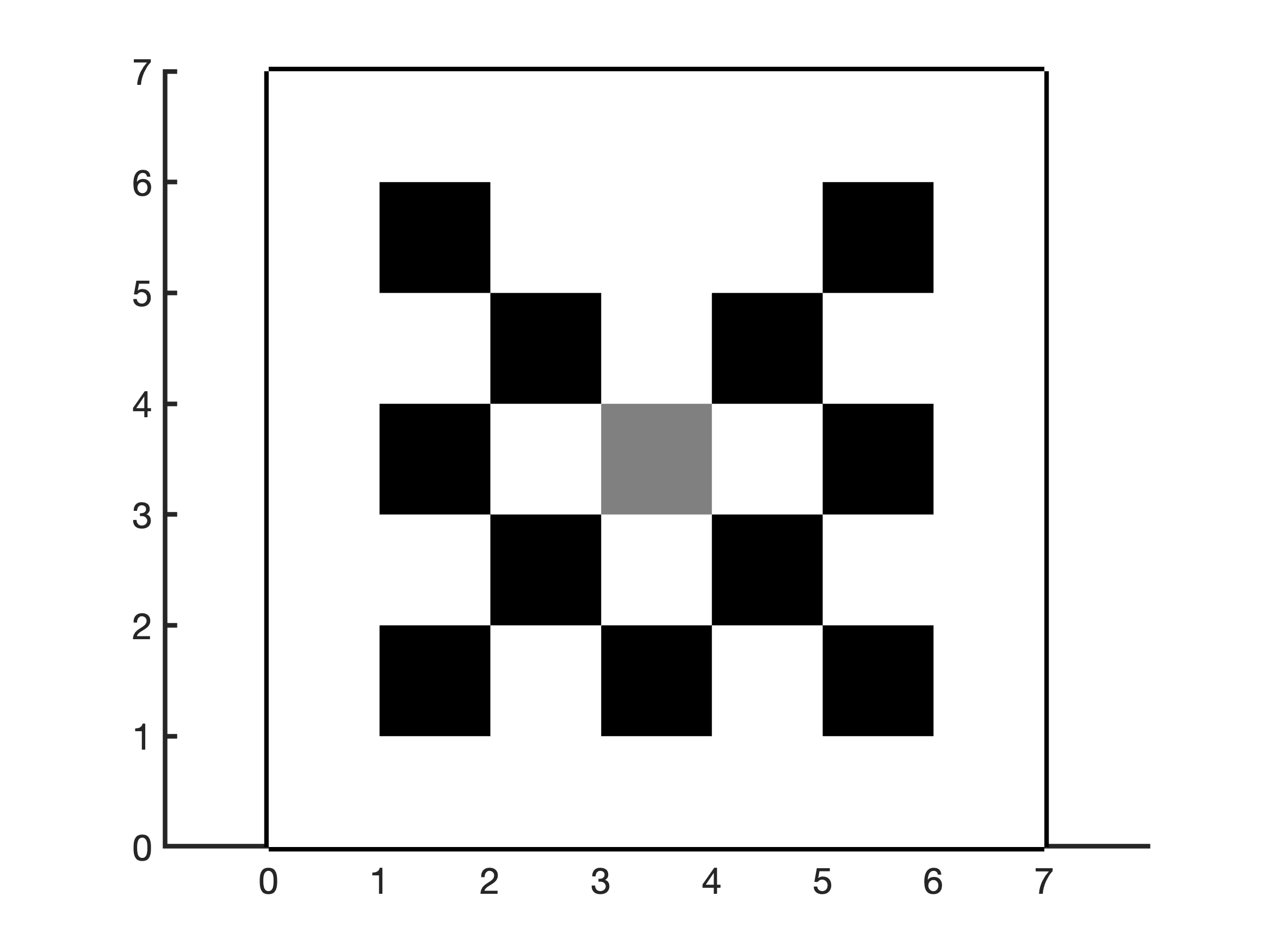
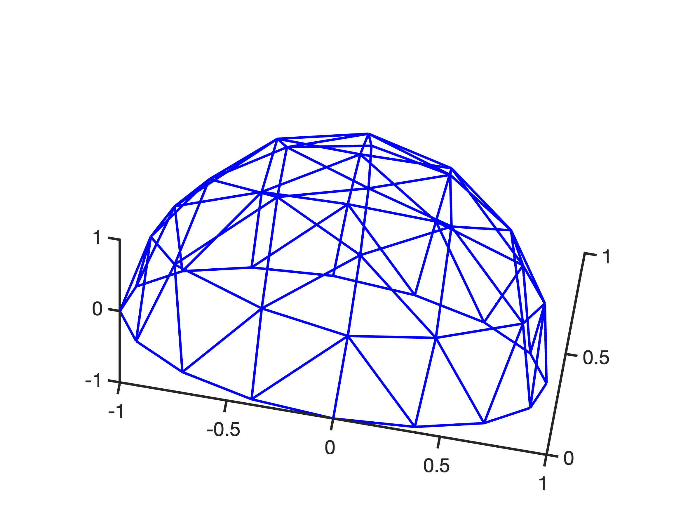
Figure 1: Left: geometry of the lattice problem in the checkerboard domain. White and grey areas are characterized by the optical parameters $\sigma_{s}=10$ and $\sigma_{a}=0.01$, while in the black zones $\sigma_{s}=0$ and $\sigma_{a}=1$. The internal source of radiation is $q=1$ in the grey square, $q=0$ outside of it. Right: Sketch of the spherical grid for the upper half sphere.

6.1 Minimization over $W_{h,N}^{c}$

We investigate the performance of the residual minimization strategy when using the subspace $W_{h,N}^{c}$ defined in Eq. 42 for different anisotropy parameters $g$. Furthermore, we investigate the behavior on the parameter $K$ in Eq. 39. Here, we choose $K=1,6,15$ such that it corresponds to the number of even spherical harmonics of degree at most $l=0,2,4$, respectively. This choice is motivated by the observation that the $2l+1$ spherical harmonics of degree $l$ are eigenfunctions of $\Theta$ with eigenvalues $g^{l}$. The resulting number of iterations are displayed in Table 1. As can be seen from the decay of the residuals depicted in Figure 2, the minimization based approach is much faster than the plain source iteration, which converges linearly with rate $\rho=0.999$. Additionally, we observe a consistent decay of the residual per iteration. Moreover, increasing $K$ yields smaller iteration counts. Since $\mathrm{dim}(W_{h,N}^{c})=1$, the subspace correction computed here pays off if the contraction rate of the residuals is better than $\rho^{2}=0.998$, cf. Remark 5.3. This is the case for all our experiments, as it is shown by the numbers in brackets in Table 1, indicating the maximum contraction rate during the corresponding iterations.

Before testing the performance of the approach on the next subspace for minimization, let us discuss Table 2, where we show the iteration counts for the choice $g=0.7$ and $K=6$, and for different angular and spatial grids obtained by successive refinements. We observe that the number of iterations varies only slightly upon mesh refinement, which we expect, because we derived the iteration from its infinite-dimensional counterpart.

Table 1: Iteration counts for minimization over $W_{h,N}^{c}$, defined in Eq. 42, for different anisotropy parameters $g$ and order $K$ of subspace correction, cf. Eq. 39.

	$g$
$K$	0.1	0.3	0.5	0.7	0.9	0.99
1	62 (0.817)	58 (0.805)	54 (0.795)	57 (0.809)	97 (0.882)	455 (0.981)
6	20 (0.532)	25 (0.603)	14 (0.377)	13 (0.371)	31 (0.706)	283 (0.973)
15	12 (0.312)	10 (0.245)	8 (0.157)	8 (0.216)	18 (0.657)	234 (0.969)

Table 2: Iteration counts for minimization over $W_{h,N}^{c}$, defined in Eq. 42, for $g=0.7$ and $K=6$, and different spatial and angular grids.

	$n_{S}^{+}$
$n_{R}^{+}$	16	64	256	1024
841	8	8	9	9
3 249	8	9	10	10
12 769	8	10	11	11
50 625	9	11	12	13

Figure 2: Residual decay for correction searched in the subspace $W_{h,N}^{c}$. From left to right, first row $g=0.1,\ 0.3,\ 0.5$; second row, $g=0.7,\ 0.9,\ 0.99$. The lines’ style refers to number of even eigenfuctions of the scattering operator employed: $K=1$ solid line; $K=6$ dotted line; $K=15$ dashed line.

6.2 Minimization over $\stackon[.5pt]{W}{\scriptscriptstyle\sim}_{h,N}^{c}$

As a second test case, we study how the residual minimization approach performs over the enriched subspace $\stackon[.5pt]{W}{\scriptscriptstyle\sim}_{h,N}^{c}$ defined in Eq. 43. As it can be seen from Table 3, for moderate values of the anisotropy factor $g$ the improvement in the number of iterations is negligible with respect to minimization on $W_{h,N}^{c}$. However, for highly forward peaked scattering, $g=0.99$, which cause the iteration to be notably slower than the other cases, the improvement is more visible, even for low order corrections ($K=1$). Figure 3 shows the convergence history of the residuals, and we observe a robust convergence behavior. Since $\mathrm{dim}(\stackon[.5pt]{W}{\scriptscriptstyle\sim}_{h,N}^{c})=4$, minimization over this subspace is useful if the contraction rate of the residuals stays below $\rho^{5}=0.995$, cf. Remark 5.3. Once again, our method achieves this requirement, as shown in brackets in Table 3.

Table 3: Iteration counts for minimization over $\stackon[.5pt]{W}{\scriptscriptstyle\sim}_{h,N}^{c}$ defined in Eq. 43 for different anisotropy parameters $g$ and order $K$ of subspace correction, cf. Eq. 39.

	$g$
$K$	0.1	0.3	0.5	0.7	0.9	0.99
1	58 (0.804)	54 (0.792)	51 (0.785)	56 (0.807)	98 (0.893)	388 (0.975)
6	18 (0.487)	22 (0.571)	12 (0.324)	13 (0.371)	26 (0.621)	123 (0.940)
15	11 (0.284)	9 (0.219)	8 (0.142)	8 (0.213)	16 (0.449)	93 (0.879)

Figure 3: Residual decay for correction searched in the subspace $\stackon[.5pt]{W}{\scriptscriptstyle\sim}_{h,N}^{c}$. From left to right, first row $g=0.1,\ 0.3,\ 0.5$; second row, $g=0.7,\ 0.9,\ 0.99$. The lines style refers to the dimension of the corrections subspace: $K=1$ solid line; $K=6$ dotted line; $K=15$ dashed line.

6.3 Minimization over $\stackon[.5pt]{W}{\scriptscriptstyle\sim}_{h,N}^{c,m}$

Exploiting Anderson-type acceleration techniques as described in Section 5.4.3 we observe a substantial reduction in the iteration count for all values of $g$ and already for moderate $m$ and low-order corrections. Indeed, comparing Table 3 and Table 4, where a history of $m=2$ iterates is taken into account for residual minimization and thus $\mathrm{dim}(\stackon[.5pt]{W}{\scriptscriptstyle\sim}_{h,N}^{c,2})=6$, we notice that already for $K=1$ the number of iterations is roughly reduced by a factor of $3$ for small $g$ and a factor of $2$ for $g$ close to $1$. The numbers in Table 5, where $m=4$ was chosen, are comparable to those in Table 4. Thus, we prefer the choice $m=2$, because it requires less memory and fewer residual computations to setup Eq. 36. Figure 4 and Figure 5 show the convergence histories for minimizing the residuals. As before the decay is consistent, i.e. the residuals are converging linearly with a rate smaller than $\rho$, see also Table 4 and Table 5 for an upper bound on this rate. As for the previous cases, since here $m=2$ corresponds to $N=6$ and $m=4$ to $N=8$, the subspace correction pays off if residual reduction per step is better than $\rho^{7}=0.993$, and $\rho^{9}=0.991$, respectively, cf. Remark 5.3 again. As shown in brackets in Table 4 and Table 5, this is always the case for our experiment.

Table 4: Iteration counts for minimization over $\stackon[.5pt]{W}{\scriptscriptstyle\sim}_{h,N}^{c,2}$ defined in Eq. 44 for different anisotropy parameters $g$ and order $K$ of subspace correction, cf. Eq. 39.

$m=2$	$g$
$K$	0.1	0.3	0.5	0.7	0.9	0.99
1	17 (0.500)	17 (0.483)	20 (0.579)	27 (0.667)	42 (0.778)	262 (0.975)
6	9 (0.224)	10 (0.237)	8 (0.172)	9 (0.210)	19 (0.518)	96 (0.937)
15	7 (0.119)	7 (0.100)	6 (0.076)	7 (0.121)	13 (0.375)	67 (0.838)

Table 5: Iteration counts for minimization over $\stackon[.5pt]{W}{\scriptscriptstyle\sim}_{h,N}^{c,4}$ defined in Eq. 44 for different anisotropy parameters $g$ and order $K$ of subspace correction, cf. Eq. 39.

$m=4$	$g$
$K$	0.1	0.3	0.5	0.7	0.9	0.99
1	16 (0.671)	17 (0.675)	17 (0.689)	22 (0.721)	39 (0.810)	218 (0.968)
6	11 (0.598)	13 (0.751)	10 (0.324)	11 (0.540)	19 (0.569)	92 (0.918)
15	9 (0.606)	10 (0.685)	9 (0.527)	8 (0.492)	13 (0.446)	63 (0.847)

Figure 4: Residual decay for correction searched in the subspace $\stackon[.5pt]{W}{\scriptscriptstyle\sim}_{h,N}^{c,2}$. From left to right, first row $g=0.1,\ 0.3,\ 0.5$; second row, $g=0.7,\ 0.9,\ 0.99$. The lines’ style refers to number of even eigenfuctions of the scattering operator employed: $K=1$ solid line; $K=6$ dotted line; $K=15$ dashed line.

Figure 5: Residual decay for correction searched in the subspace $\stackon[.5pt]{W}{\scriptscriptstyle\sim}_{h,N}^{c,4}$. From left to right, first row $g=0.1,\ 0.3,\ 0.5$; second row, $g=0.7,\ 0.9,\ 0.99$. The lines’ style refers to number of even eigenfuctions of the scattering operator employed: $K=1$ solid line; $K=6$ dotted line; $K=15$ dashed line.

7 Conclusions and discussion

In this paper we have developed a generic and flexible strategy to accelerate the source iteration for the solution of anisotropic radiative transfer problems using residual minimization. We showed convergence of the resulting method for any choice of subspace employed in the residual minimization. The flexibility in choosing the subspace was used to exploit higher order diffusion corrections, which were shown to be effective for highly forward peaked scattering. Moreover, the numerical results confirmed that the required iteration counts do depend on the discretization only mildly.

We mention that our approach can be seen as a two-level scheme. We leave it to future work to extended it and compare it to angular multilevel schemes. Moreover, the analysis of the precise approximation properties of the considered subspaces is also left to future research. We close by mentioning that the efficient and robust solution of the source problem Eq. 1 is also relevant for solving eigenvalue problems, see, e.g., [6, 4, 26].

References

- [1] M. L. Adams and E. W. Larsen, Fast iterative methods for discrete-ordinates particle transport calculations, Prog. Nuclear Energy, 40 (2002), pp. 3–159, https://doi.org/10.1016/S0149-1970(01)00023-3.
- [2] D. Y. Anistratov and J. S. Warsa, Discontinuous finite element quasi-diffusion methods, Nuclear Science and Engineering, 191 (2018), pp. 105–120, https://doi.org/10.1080/00295639.2018.1450013.
- [3] S. R. Arridge and J. C. Schotland, Optical tomography: forward and inverse problems, Inverse Problems, 25 (2009), pp. 123010, 59, https://doi.org/10.1088/0266-5611/25/12/123010.
- [4] A. P. Barbu and M. L. Adams, Convergence properties of a linear diffusion-acceleration method for k-eigenvalue transport problems, Nuclear Science and Engineering, 197 (2022), pp. 517–533, https://doi.org/10.1080/00295639.2022.2123205.
- [5] T. A. Brunner, Forms of approximate radiation transport, in Nuclear Mathematical and Computational Sciences: A Century in Review, A Century Anew Gatlinburg, LaGrange Park, IL, 2003, American Nuclear Society. Tennessee, April 6-11, 2003.
- [6] M. T. Calef, E. D. Fichtl, J. S. Warsa, M. Berndt, and N. N. Carlson, Nonlinear Krylov acceleration applied to a discrete ordinates formulation of the k-eigenvalue problem, Journal of Computational Physics, 238 (2013), pp. 188–209, https://doi.org/https://doi.org/10.1016/j.jcp.2012.12.024.
- [7] K. M. Case and P. F. Zweifel, Existence and uniqueness theorems for the neutron transport equation, Journal of Mathematical Physics, 4 (1963), pp. 1376–1385, https://doi.org/10.1063/1.1703916.
- [8] K. M. Case and P. F. Zweifel, Linear transport theory, Addison-Wesley Publishing Co., Reading, Mass.-London-Don Mills, Ont., 1967.
- [9] S. Dargaville, A. Buchan, R. Smedley-Stevenson, P. Smith, and C. Pain, A comparison of element agglomeration algorithms for unstructured geometric multigrid, Journal of Computational and Applied Mathematics, 390 (2021), p. 113379, https://doi.org/https://doi.org/10.1016/j.cam.2020.113379.
- [10] J. Dölz, O. Palii, and M. Schlottbom, On robustly convergent and efficient iterative methods for anisotropic radiative transfer, J. Sci. Comput., 90 (2022), https://doi.org/10.1007/s10915-021-01757-9.
- [11] H. Egger and M. Schlottbom, A mixed variational framework for the radiative transfer equation, Math. Models Methods Appl. Sci., 22 (2012), pp. 1150014, 30, https://doi.org/10.1142/S021820251150014X.
- [12] H. Egger and M. Schlottbom, An Lp theory for stationary radiative transfer, Applicable Analysis, 93 (2013), pp. 1283–1296, https://doi.org/10.1080/00036811.2013.826798.
- [13] K. F. Evans, The spherical harmonics discrete ordinate method for three-dimensional atmospheric radiative transfer, J. Atmospheric Sci., 55 (1998), pp. 429–446, https://doi.org/10.1175/1520-0469(1998)055<0429:TSHDOM>2.0.CO;2.
- [14] T. S. Haut, B. S. Southworth, P. G. Maginot, and V. Z. Tomov, Diffusion synthetic acceleration preconditioning for discontinuous Galerkin discretizations of transport on high-order curved meshes, SIAM J. Sci. Comput., 42 (2020), pp. B1271–B1301, https://doi.org/10.1137/19M124993X.
- [15] H. Hensel, R. Iza-Teran, and N. Siedow, Deterministic model for dose calculation in photon radiotherapy, Phys. Med. Biol., 51 (2006), pp. 675–693, https://doi.org/10.1088/0031-9155/51/3/013.
- [16] G. Kanschat and J.-C. Ragusa, A robust multigrid preconditioner for -DG approximation of monochromatic, isotropic radiation transport problems, SIAM Journal on Scientific Computing, 36 (2014), pp. A2326–A2345, https://doi.org/10.1137/13091600x, http://dx.doi.org/10.1137/13091600X.
- [17] B. Lee, A novel multigrid method for Sn discretizations of the mono-energetic Boltzmann transport equation in the optically thick and thin regimes with anisotropic scattering, part i, SIAM Journal on Scientific Computing, 31 (2010), pp. 4744–4773, https://doi.org/10.1137/080721480, http://dx.doi.org/10.1137/080721480.
- [18] G. I. Marchuk and V. I. Lebedev, Numerical methods in the theory of neutron transport, Harwood Academic Publishers, Chur, second ed., 1986.
- [19] X. Meng, S. Wang, G. Tang, J. Li, and C. Sun, Stochastic parameter estimation of heterogeneity from crosswell seismic data based on the Monte Carlo radiative transfer theory, J. Geophys. Eng., 14 (2017), pp. 621–633, https://doi.org/10.1088/1742-2140/aa6130.
- [20] S. Olivier, W. Pazner, T. S. Haut, and B. C. Yee, A family of independent variable eddington factor methods with efficient preconditioned iterative solvers, Journal of Computational Physics, 473 (2023), p. 111747, https://doi.org/https://doi.org/10.1016/j.jcp.2022.111747.
- [21] O. Palii and M. Schlottbom, On a convergent DSA preconditioned source iteration for a DGFEM method for radiative transfer, Comput. Math. Appl., 79 (2020), pp. 3366–3377, https://doi.org/10.1016/j.camwa.2020.02.002.
- [22] J. Ragusa, J.-L. Guermond, and G. Kanschat, A robust SN-DG-approximation for radiation transport in optically thick and diffusive regimes, Journal of Computational Physics, 231 (2012), pp. 1947–1962, https://doi.org/https://doi.org/10.1016/j.jcp.2011.11.017.
- [23] J. C. Ragusa and Y. Wang, A two-mesh adaptive mesh refinement technique for neutral-particle transport using a higher-order DGFEM, J. Comput. Appl. Math., 233 (2010), pp. 3178–3188, https://doi.org/10.1016/j.cam.2009.12.020.
- [24] T. P. Robitaille, Hyperion: an open-source parallelized three-dimensional dust continuum radiative transfer code, A&A, 536 (2011), p. A79, https://doi.org/10.1051/0004-6361/201117150.
- [25] M. Rustamzhon, D. Press, G. K. Baskaran, S. Sadeghi, and S. Nizamoglu, Unravelling radiative energy transfer in solid-state lighting, J. Appl. Phys., 123 (2018), https://doi.org/10.1063/1.5008922.
- [26] Q. Shen and B. Kochunas, Practical considerations for the adoption of Anderson acceleration in nonlinear diffusion accelerated transport, Annals of Nuclear Energy, 199 (2024), p. 110330, https://doi.org/10.1016/j.anucene.2023.110330.
- [27] Q. Sheng and C. D. Hauck, Uniform convergence of an upwind discontinuous Galerkin method for solving scaled discrete-ordinate radiative transfer equations with isotropic scattering, Mathematics of Computation, 90 (2021), pp. 2645–2669, https://doi.org/10.1090/mcom/3670.
- [28] B. S. Southworth, M. Holec, and T. S. Haut, Diffusion synthetic acceleration for heterogeneous domains, compatible with voids, Nuclear Science and Engineering, 195 (2020), pp. 119–136, https://doi.org/10.1080/00295639.2020.1799603.
- [29] K. Stamnes, G. Thomas, and J. Stamnes, Radiative transfer in the atmosphere and ocean, Modeling and Simulation in Science, Engineering and Technology, Cambridge University Press, 2nd ed., 2017, https://doi.org/10.1017/9781316148549.
- [30] Z. Sun and C. D. Hauck, Low-memory, discrete ordinates, discontinuous Galerkin methods for radiative transport, SIAM Journal on Scientific Computing, 42 (2020), pp. B869–B893, https://doi.org/10.1137/19m1271956.
- [31] B. Turcksin, J. C. Ragusa, and J. E. Morel, Angular multigrid preconditioner for Krylov-based solution techniques applied to the Sn equations with highly forward-peaked scattering, Transport Theory and Statistical Physics, 41 (2012), pp. 1–22, https://doi.org/10.1080/00411450.2012.672944.
- [32] H. F. Walker and P. Ni, Anderson acceleration for fixed-point iterations, SIAM Journal on Numerical Analysis, 49 (2011), pp. 1715–1735, https://doi.org/10.1137/10078356x.
- [33] J. S. Warsa and D. Y. Anistratov, Two-level transport methods with independent discretization, Journal of Computational and Theoretical Transport, 47 (2018), pp. 424–450, https://doi.org/10.1080/23324309.2018.1497991.
- [34] J. S. Warsa, T. A. Wareing, and J. E. Morel, Krylov iterative methods and the degraded effectiveness of diffusion synthetic acceleration for multidimensional SN calculations in problems with material discontinuities, Nuclear Science and Engineering, 147 (2004), pp. 218–248, https://doi.org/10.13182/nse02-14.
- [35] J. Willert, H. Park, and W. Taitano, Using Anderson acceleration to accelerate the convergence of neutron transport calculations with anisotropic scattering, Nuclear Science and Engineering, 181 (2015), pp. 342–350, https://doi.org/10.13182/nse15-16.