Block-Additive Gaussian Processes under Monotonicity Constraints

Abstract

We generalize the additive constrained Gaussian process framework to handle interactions between input variables while enforcing monotonicity constraints everywhere on the input space. The block-additive structure of the model is particularly suitable in the presence of interactions, while maintaining tractable computations. In addition, we develop a sequential algorithm, MaxMod, for model selection (i.e., the choice of the active input variables and of the blocks). We speed up our implementations through efficient matrix computations and thanks to explicit expressions of criteria involved in MaxMod. The performance and scalability of our methodology are showcased with several numerical examples in dimensions up to 120, as well as in a 5D real-world coastal flooding application, where interpretability is enhanced by the selection of the blocks.

1 Introduction

Constrained Gaussian processes (GPs).

GPs are a central tool within the family of non-parametric Bayesian models, offering significant theoretical and computational advantages [1]. They have been successfully applied in various research fields, including numerical code approximations [2], global optimization [3, 4], model calibration [5], geostatistics [6, 7] and machine learning [1].

It is well-known that accounting for inequality constraints (e.g. boundedness, monotonicity, convexity) in GPs enhances prediction accuracy and yields more realistic uncertainties [8, 9, 10, 11, 12]. These constraints correspond to available information on functions over which GP priors are considered. Constraints such us positivity and monotonicity appear in diverse research fields, including social system analysis [13], computer networking [14], econometrics [15], geostatistics [16], nuclear safety criticality assessment [17], tree distributions [18], coastal flooding [19], and nuclear physics [20]. The diversity of these domains highlights the versatility and relevance of constrained GPs.

In this paper, we consider the finite-dimensional framework of GPs introduced in [16, 17] to handle constraints using multi-dimensional “hat basis” functions locally supported around knots of a grid. In dimension one, these hat basis functions are also known as splines of degree one or $\mathbb{P}_{1}$ finite element basis functions. Importantly, this framework guarantees that constraints are satisfied everywhere in the input space. However, when applying these constrained GP models to a target function $y:[0,1]^{D}\to\mathbb{R}$, one encounters the “curse of dimensionality”, since the multi-dimensional hat basis functions are built by tensorization of the one-dimensional ones. [21] alleviates this issue by introducing the MaxMod algorithm, which performs variable selection and optimized knot allocation. MaxMod was successfully applied to target functions up to dimension $D=20$ (though with fewer active variables).

Constrained additive GPs.

In the general statistics literature, a common approach to achieve dimensional scalability is to assume additive target functions:

$$y(x_{1},\ldots,x_{D})=y_{1}(x_{1})+\cdots+y_{D}(x_{D}).$$ (1)

Although this assumption may lead to overly “rigid” models, it results in simple frameworks that easily scale in high dimensions, as seen in [22, 23] (without inequality constraints). Additive (unconstrained) GPs are considered in [24, 25], as sums of one-dimensional independent GPs. We note that, besides computational advantages, the additive assumption also yields interpretability, such as the assessment of individual effects of input variables.

In [26], constrained additive GPs are suggested based on the finite-dimensional approximation, providing a significant scaling to [21], up to hundreds of dimensions. Furthermore, MaxMod has been adapted for variable selection and knot allocation.

Extension to block-additive GPs (baGPs).

In this paper, we seek a “best of both worlds” trade-off between [21], which is more flexible but does not scale with dimension, and [26], which scales better but cannot handle interactions between variables. Thus we suggest a block-additive structure, yielding block-additive GPs (baGPs). More precisely, we consider functions $[0,1]^{D}\to\mathbb{R}$:

$$y(x_{1},\ldots,x_{D})=y_{1}(\bm{x}_{\mathcal{B}_{1}})+\cdots+y_{B}(\bm{x}_{\mathcal{B}_{B}}).$$ (2)

Here, $\mathcal{P}:=\{\mathcal{B}_{1},\ldots,\mathcal{B}_{B}\}$ represents a sub-partition of $\{1,\ldots,D\}$, where the disjoint union of the sets $\mathcal{B}_{j}$ satisfies $\bigsqcup_{j=1}^{B}\mathcal{B}_{j}\subset\{1,\ldots,D\}$. The subset of variables $\bm{x}_{\mathcal{B}_{j}}$ is simply obtained from $\bm{x}$ by keeping the components of indices in $\mathcal{B}_{j}$.

The block-additive model offers flexibility in choosing the partition $\mathcal{P}$, thereby encompassing both additive functions and functions with interactions at any order among all input variables. Its practical utility is especially relevant when the sizes of the blocks $|\mathcal{B}_{j}|$, equivalently the interaction orders, remain relatively small. In our constrained framework, this enhances the tractability of optimization and Monte Carlo sampling needed to compute the constrained GP posterior.

In practice, the block structure is unknown, but evaluations of the target function $y$ are available. Therefore, we propose a data-driven approach to select the blocks by providing an extension of the MaxMod algorithm. It is worth noting that outside of the GP world, the setting of block-additive models and methods for selecting blocks have been studied in the statistics literature, see for instance [27, 28, 29]. In particular, the ACOSSO method in [27] is closest to GPs as it relies on reproducing kernel Hilbert spaces (RKHSs), but does not handle inequality constraints. Our extension of MaxMod is the first block selection method tailored to constrained GPs, to the best of our knowledge.

Summary of contributions.

In this paper, we consider a general target function $y$, known to belong to a convex set. We will focus on the convex set of componentwise monotonic (e.g. non-decreasing) functions. Nevertheless, as discussed in Remark 4, our framework can handle other convex sets for constraints such as componentwise convexity.

We make the following contributions.

1) We introduce a comprehensive framework for handling baGPs and constrained baGPs. Theoretical results are derived for multi-dimensional hat-basis functions. In particular, we explicitly provide the change-of-basis matrices corresponding to adding active variables, merging blocks or adding knots. We also use the matrix inversion lemma [1] to reduce the computational complexity.

2) We extend MaxMod to the block-additive setting, as discussed above. This algorithm maximizes a criterion based on the modification of the maximum a posteriori (MAP) predictor between consecutive iterations, hence its name MaxMod. For computational efficiency, we derive an explicit expression of the MaxMod criterion.

3) We provide predictors for every block-function $y_{i}$ in (2) up to an additive constant (see Remark 2). The benefit for interpretability is highlighted on a real-world 5D coastal flooding problem previously studied [30, 19, 21].

4) We demonstrate the scalability and performance of our methodology on numerical examples up to dimension 120. Our results confirm that MaxMod identifies the most influential input variables, making it efficient for dimension reduction while ensuring accurate models that satisfy the constraints everywhere on the input space. In the coastal flooding application, compared to [21], our approach achieves higher accuracy with fewer knots.

5) We provide open-source codes in the GitHub repository: https://github.com/anfelopera/lineqGPR.

Structure of the paper.

Section 2 provides a high-level overview of the theoretical concepts leading to the construction of our method. Section 3 details the construction of the finite-dimensional baGPs and the computation of their posteriors. Section 4 introduces the MaxMod algorithm. Section 5 presents the numerical results on toy examples and the 5D coastal flooding application. Finally, Section 6 summarizes the conclusions and potential future work.

2 Overview over the block-additive MaxMod method

To construct a partition that defines the block-additive structure of $y$ specified in (2), we sequentially increment sub-partitions $\mathcal{P}=\{\mathcal{B}_{1},\ldots,\mathcal{B}_{B}\}$. For clarity and consistency, we maintain the terms $\mathcal{P}$, $\mathcal{B}_{j}$ and $B$, presented in the introduction. We emphasize that these parameters are adjustable during each iteration of the MaxMod algorithm. Initially, the sub-partition $\mathcal{P}$ consists of a single block $\mathcal{B}_{1}$ containing one variable $i\in\{1,\ldots,D\}$. The sets $\mathcal{B}_{j}$ correspond to active variables interacting together in $y$’s output. Therefore, the sub-partition $\mathcal{P}$ defines the “shape” (i.e. the block-additive structure) of our Gaussian prior, denoted as $Y^{\mathcal{P}}$ (explained in detail in Section 3.1):

$$Y^{\mathcal{P}}(x_{1},\ldots,x_{D})=Y_{1}(\bm{x}_{\mathcal{B}_{1}})+\cdots+Y_{B}(\bm{x}_{\mathcal{B}_{B}}),$$ (3)

where the $Y_{j}$’s are independents GPs defined over $[0,1]^{|\mathcal{B}_{j}|}$. In line with [21, 26], we deal with finite-dimensional approximations of the independent GPs, that we will refer to as finite-dimensional GPs. We define $X^{(i)}=[0,1]$ for $i\in\{1,\ldots,D\}$, $X=X^{(1)}\times\cdots\times X^{(D)}$ and $y\in E=\mathcal{C}^{0}(X,\mathbb{R})$ the set of continuous functions from $X$ to $\mathbb{R}$.

According to [31], the condition that $y$ belongs to a convex set $\mathcal{C}\subset\mathcal{C}^{0}(X,\mathbb{R})$ is addressed using finite-dimensional approximation processes of $Y^{\mathcal{P}}$, and considering their limit. This approximation is a sequential projection of the GP $Y^{\mathcal{P}}$ over finite-dimensional sets. In practice, these sets are constructed from increasing families of non-symmetric hat basis functions $(\beta_{m})_{m\geq 0}$ associated with their finite-dimensional subspaces $E_{m}=\operatorname{span}(\beta_{m})$. These families are derived from one-dimensional hat basis function (see Figure 1). Further details are given in Section 3.2.1.

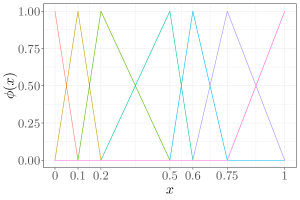
Figure 1: The panels show an example of (left) a one-dimensional hat basis generated from a subdivision $s=\{0,0.1,0.2,0.5,0.6,0.75,1\}$, and (right) an example of the projection (in blue) of a function (in red) onto the vector space generated by the hat family illustrated in the left panel.

The basis $\beta_{m}$ is constructed using tensorization of one-dimensional hat basis families, more details are provided in Section 3.2.2, we give here the main ideas. For every $i\in\{1,\ldots,D\}$ we have a basis $\beta^{(i)}_{m}$ in $\mathcal{C}^{0}(X^{(i)},\mathbb{R})$. Then, for every $\mathcal{B}_{j}$, $j\in\{1,\ldots,B\}$, we define a tensorized hat basis $(\beta^{\mathcal{B}_{j}}_{m})_{m\geq 0}$ as the set of functions $\phi^{j}_{m}:X\to\mathbb{R}$:

$$\phi^{j}_{m}(x_{1},\ldots,x_{D}):=\prod_{i\in\mathcal{B}_{j}}\phi^{(i)}_{m}(x_{i}),\hskip 28.45274pt\phi^{(i)}_{m}\in\beta^{(i)}_{m},\,\forall i\in\{1,\ldots,D\}.$$ (4)

Note that functions in $\beta^{\mathcal{B}_{j}}_{m}$ are essentially functions defined on $X^{\mathcal{B}_{j}}:=\prod_{i\in\mathcal{B}_{j}}X^{(i)}$. Thus, the functions in $E_{m}^{\mathcal{P}}=\operatorname{span}(\beta^{\mathcal{B}_{1}}_{m}\cup\cdots\cup\beta^{\mathcal{B}_{B}}_{m})$ have the shape of (2). The projection $\widetilde{Y}_{m}$ of $Y^{\mathcal{P}}$ onto the $E_{m}^{\mathcal{P}}$ is a finite-dimensional GP and can be written as:

$$\widetilde{Y}_{m}(\bm{x}):=P_{E_{m}^{\mathcal{P}}}\left(Y^{\mathcal{P}}\right)(\bm{x})=\sum_{j=1}^{B}\sum_{\phi_{j}\in\beta^{\mathcal{B}_{j}}_{m}}\xi_{\phi_{j}}\phi_{j}(\bm{x}),$$ (5)

where the $\xi_{\phi_{j}}$’s are Gaussian coefficients. Details over the projection $P_{E_{m}^{\mathcal{P}}}$ can be found in Section 3.2.3. We will assume in the rest of the paper that we have an order in our basis $(\beta^{\mathcal{B}_{1}}_{m},\ldots,\,\beta^{\mathcal{B}_{B}}_{m})$ so that we can define the Gaussian random vector $\bm{\xi}=(\xi_{\phi_{j}})_{j\in\{1,\ldots,B\},\phi_{j}\in\beta^{\mathcal{B}_{j}}_{m}}$. We set as well for $\bm{x}\in X$, the vector $\bm{\Phi}(\bm{x})=(\phi_{j}(\bm{x}))_{j\in\{1,\ldots,B\},\phi_{j}\in\beta^{\mathcal{B}_{j}}_{m}}$, we can rewrite $\widetilde{Y}_{m}(\bm{x})=\bm{\xi}^{\top}\bm{\Phi}(\bm{x})$. This formulation underlines an important fact: conditioning $\widetilde{Y}_{m}$ is equivalent of conditioning $\bm{\xi}$ that is an easier problem.

Writing $\bm{X}=[\bm{x}^{(1)},\ldots,\bm{x}^{(n)}]^{\top}$ and $\bm{Y}=[y^{(1)},\ldots,y^{(n)}]^{\top}$ the observations, $y(\bm{x}^{(i)})+\epsilon_{i}=y^{(i)}$ for $i$ in $\{1,\ldots,D\}$, $\epsilon_{i}$ is a Gaussian noise of variance $\tau^{2}$ independent of GPs $Y_{j}$ . Writing $\bm{\epsilon}=[\epsilon_{1},\ldots,\epsilon_{n}]^{\top}\sim\mathcal{N}(0,\tau^{2}\bm{I}_{n})$, one can define the truncated Gaussian vector:

$$\left(\bm{\xi}\big{|}\widetilde{Y}_{m}(\bm{X})+\bm{\epsilon}=\bm{Y},\widetilde{Y}_{m}\in\mathcal{C}\right).$$ (6)

From [31], a good predictor of $y$ is $\widehat{Y}_{m}=\widehat{\bm{\xi}}^{\top}\bm{\Phi}$ where $\widehat{\bm{\xi}}$ is the maximum a posterior (MAP) estimator, denoted as the maximum of distribution estimator (mode) of the conditional vector in (6). The mean a posteriori (mAP) estimator has been studied in [32, 19, 33] and is also relevant, but presents difficulties to be computed due to Monte Carlo routines. We will focus on the MAP estimator in this paper. Suppose there exists a $\mathcal{C}^{\prime}\subset\mathbb{R}^{|\beta^{\mathcal{B}_{1}}_{m}\cup\cdots\cup\beta^{\mathcal{B}_{B}}_{m}|}$ a convex set (detailed in Section 3.4) such that the following equivalence holds:

$$\widetilde{Y}_{m}\in\mathcal{C}\Longleftrightarrow\bm{\xi}\in\mathcal{C}^{\prime}.$$ (7)

Then, the mode $\widehat{\bm{\xi}}$ is solution of the following quadratic optimization problem:

$$\widehat{\bm{\xi}}=\underset{\bm{\xi}\in\mathcal{C}^{\prime}}{\arg\min}\,(\bm{\xi}-\bm{\mu})^{\top}\bm{\Sigma}^{-1}(\bm{\xi}-\bm{\mu}).$$ (8)

Here, $\bm{\mu}$ and $\bm{\Sigma}$ are the mean and the covariance matrix of the Gaussian vector $(\bm{\xi}|\,\bm{\xi}^{\top}\bm{\Phi}(\bm{X})+\bm{\epsilon}=\bm{Y})$ (see section 3.3). Methods to solve (8) have been studied in [21, 26], notice that the complexity of (8) depends on the dimension of the space $E^{\mathcal{P}}_{m}$: $|\beta^{\mathcal{B}_{1}}_{m}\cup\cdots\cup\beta^{\mathcal{B}_{B}}_{m}|$.

From bases $(\beta^{(i)}_{m})_{1\leq i\leq D}$ and a sub-partition $\mathcal{P}$ we can compute the predictor $\widetilde{Y}_{m}$ of $y$ taking into account given observations $(\bm{X},\bm{Y})$ and the fact that $y$ lies in a convex $\mathcal{C}$. However, one can notice that the predictor lies into $E_{m}$ so that $\|y-\widehat{Y}_{m}\|\geq d(y,E_{m})$, therefore the choice of the bases $(\beta^{(i)}_{m})_{1\leq i\leq D}$ and partition $\mathcal{P}$ is crucial for the accuracy of our predictor. The purpose of the MaxMod is to “cleverly” update the bases $\beta_{m}$ so the one-dimensional bases and the sub-partition. The couple $((\beta^{(i)}_{m})_{i},\mathcal{P})$ is updated chosing the couple $((\beta^{(i)})_{i},\mathcal{J})$ in a set $\mathcal{M}^{\star}$ maximizing a criterion $\mathcal{K}$:

$$\left((\beta^{(i)}_{m+1})_{i},\,\mathcal{P}^{\star}\right)=\underset{((\beta^{(i)})_{i},\mathcal{J})\in\mathcal{M}^{\star}}{\arg\max}\,\mathcal{K}\left(\left((\beta^{(i)})_{i},\mathcal{J}\right),\,\left((\beta^{(i)}_{m})_{i},\mathcal{P}\right)\right).$$ (9)

For the couples in the set $\mathcal{M}^{\star}$, we essentially have three choices: activating a variable $i$, incrementing a basis $\beta^{(i)}_{m}$ or merging two blocks $\mathcal{B}_{j_{1}}$ and $\mathcal{B}_{j_{2}}$. Basically, $\mathcal{K}$ aims to quantify the information “gained” by extending $\widetilde{Y}^{\mathcal{P}}_{\beta_{m}}$ to $\widetilde{Y}^{\mathcal{P}^{\star}}_{\beta_{m+1}}$ while penalizing by the dimension increment between $E^{\mathcal{P}}_{\beta_{m}}$ and the next function space $E^{\mathcal{\mathcal{P}^{\star}}}_{\beta_{m+1}}$. A closed-form expression of the criterion $\mathcal{K}$ together with the detailed over the set $\mathcal{M}^{\star}$ are given in Section 4.

3 Block-additive GPs and their finite-dimensional approximations

In this section, we delve into the explicit construction of the hat basis $\beta_{m}$ introduced in Section 2. For readability, we omit the index $m$, which is not required for this construction. We will focus on the finite-dimensional constrained baGP for a given basis and sub-partition.

3.1 Block-additive GPs

As discussed in Section 2, we place GP priors over the functions $y_{1},\ldots,y_{B}$, which leads to (3). Set a sub-partition $\mathcal{P}=\{\mathcal{B}_{1},\ldots,\mathcal{B}_{B}\}$ of $\{1,\ldots,D\}$. For all $j\in\{1,\ldots,B\}$, let $\{Y_{j}(\bm{x}),\,\bm{x}\in[0,1]^{|\mathcal{B}_{j}|}\}$ be a centered GP with kernel $k_{j}$. An example of a kernel $k_{j}$ is

$$k_{j}(\bm{x}_{\mathcal{B}_{j}},\bm{x}_{\mathcal{B}_{j}}^{\prime})=\sigma^{2}_{j}\prod_{i\in\mathcal{B}_{j}}r_{\theta_{i}}(x_{i},x^{\prime}_{i}),$$ (10)

where $\bm{x}_{\mathcal{B}_{j}}=(x_{i})_{i\in\mathcal{B}_{j}}$, $\bm{x}^{\prime}_{\mathcal{B}_{j}}=(x^{\prime}_{i})_{i\in\mathcal{B}_{j}}$, and $r_{\theta_{i}}$ are the normalized one-dimensional matérn kernel:

$$r_{\theta}(x,x^{\prime})=\left(1+\sqrt{5}\frac{|x-x^{\prime}|}{\theta}+\frac{5}{3}\frac{|x-x^{\prime}|^{2}}{\theta^{2}}\right)\exp\left(-\sqrt{5}\frac{|x-x^{\prime}|}{\theta}\right).$$

For this particular kernel structure, each block has one variance parameter $\sigma_{j}^{2}\in\mathbb{R}^{+}$ and one length-scale parameter per dimension, denoted $\theta_{i}\in\mathbb{R}^{+}$. This results in a total of $B+D$ covariance parameters.

Assuming that $(Y_{j})_{1\leq j\leq B}$ are independent, then $Y^{\mathcal{P}}$ is also a centered GP with kernel $k_{\mathcal{P}}:[0,1]^{D}\times[0,1]^{D}\to\mathbb{R}$:

$$k_{\mathcal{P}}(\bm{x},\bm{x}^{\prime})=\sum_{j=1}^{B}k_{j}(\bm{x}_{\mathcal{B}_{j}},\bm{x}_{\mathcal{B}_{j}}^{\prime}),$$ (11)

for every $\bm{x},\bm{x}^{\prime}\in[0,1]^{|\mathcal{B}_{j}|}$.

The GP $Y^{\mathcal{P}}$ can be considered as a prior over the latent function $y=y_{1}\oplus\cdots\oplus y_{B}$. Let us recall $\bm{X}=[\bm{x}^{(1)},\ldots,\bm{x}^{(n)}]^{\top}$, $\bm{Y}=[y^{(1)},\ldots,\,y^{(n)}]^{\top}$, being observations of the function $y$ with $y(\bm{x}^{(i)})+\epsilon_{i}=y^{(i)}$ and $\epsilon=[\epsilon_{1},\ldots,\,\epsilon_{n}]^{\top}\sim\mathcal{N}(0,\tau^{2}\bm{I}_{n})$ independent of $Y^{\mathcal{P}}$. We can define the conditional GP

$$\{(Y^{\mathcal{P}}(\bm{x})|Y^{\mathcal{P}}(\bm{X})+\bm{\epsilon}=\bm{Y}),\,\bm{x}\in[0,1]^{D}\},$$

where the mean function $\mu$ and kernel $c$ are given by

$$\mu(\bm{x}) =k_{\mathcal{P}}(\bm{x},\bm{X})[k_{\mathcal{P}}(\bm{X},\bm{X})+\tau^{2}\bm{I}_{n}]^{-1}\bm{Y},$$ (12)

$$c(\bm{x},\bm{x}^{\prime}) =k_{\mathcal{P}}(\bm{x},\bm{x}^{\prime})-k_{\mathcal{P}}(\bm{x},\bm{X})[k_{\mathcal{P}}(\bm{X},\bm{X})+\tau^{2}\bm{I}_{n}]^{-1}k_{\mathcal{P}}(\bm{X},\bm{x}^{\prime}).$$

Here, for all vectors $\bm{a}=[a_{1},\ldots,\,a_{n}]^{\top}\in A^{n}$, $\bm{b}=[b_{1},\dots,b_{m}]^{\top}\in B^{m}$ and all function $k:A\times B\to\mathbb{R}$, the notation $k(\bm{a},\bm{b})$ corresponds to the matrix in $M_{n,m}(\mathbb{R})$, $k(\bm{a},\bm{b})=(k(a_{i},b_{j}))_{1\leq i\leq n,\\ 1\leq j\leq m}$.

We note that handling the constraint $Y^{\mathcal{P}}\in\mathcal{C}$ is challenging as $Y^{\mathcal{P}}$ is infinite-dimensional. Thus, we approximate $Y^{\mathcal{P}}$ by a finite-dimensional one, enabling to benefit from (7), that is characterizing the (functional) constraints by equivalent finite-dimensional ones.

3.2 Finite-dimensional approximation

We first define the hat basis functions, starting from the one-dimensional case. Then, we define the corresponding finite-dimensional approximation of $Y^{\mathcal{P}}$, obtained by projection.

3.2.1 One-dimensional hat basis functions

The one-dimensional hat basis functions are defined from a subdivision of $[0,1]$. Let $s$ be this subdivision: $s=(t_{1},\ldots,t_{m})$ with $t_{1}=0<\dots<t_{m}=1$. We write $\widehat{\phi}_{u,v,w}:[0,1]\to\mathbb{R}$, for $u<v<w$, the hat function with support $[u,w]$ having two linear components on $[u,v]$ and $[v,w]$, and equal to $1$ at $v$. More precisely,

$$\widehat{\phi}_{u,v,w}(x)=\begin{cases}\dfrac{x-u}{v-u}&\mbox{if }u\leq x\leq v,\\ \dfrac{w-x}{w-v}&\mbox{if }v\leq x\leq w,\\ 0&\mbox{otherwise}.\end{cases}$$

The basis created by the subdivision $s$ is then

$$\beta_{s}=\{\phi^{s}_{1},\ldots,\phi^{s}_{m}\},\hskip 28.45274pt\phi^{s}_{i}:=\widehat{\phi}_{t_{i-1},t_{i},t_{i+1}},\,1\leq i\leq m,$$ (13)

By convention, we set $t_{0}=-1$ and $t_{m+1}=2$. Note that for every $u<v<w$, $\widehat{\phi}_{u,v,w}$ can be seen as a function from $[0,1]$ just by considering its restriction to the segment.

3.2.2 Multi-dimensional hat basis functions

As in Section 2, denote $X=X^{(1)}\times\cdots\times X^{(D)}$ with $X^{(i)}=[0,1]$. For $i=1,\ldots,D$, let $s^{(i)}=\{t^{(i)}_{1},\ldots,t^{(i)}_{m^{(i)}}\}$ be a subdivision of $[0,1]$ and define the set of all subdivisions, $\mathcal{S}=\{s^{(1)},\ldots,s^{(D)}\}$ . Each $s^{(i)}$ generate a hat function basis $\beta^{(i)}$ defined in (13):

$$\beta_{s^{(i)}}:=\{\phi^{s^{(i)}}_{1},\ldots,\phi^{s^{(i)}}_{m^{(i)}}\},$$

with $m^{(i)}=|s^{(i)}|$. We consider blocks of variables $\mathcal{B}_{j}$ for all $j=1,\ldots,B$. From the block $\mathcal{B}_{j}$, we can define the multi-dimensional basis $\beta^{\mathcal{S}}_{\mathcal{B}_{j}}$ as:

$$\beta^{\mathcal{S}}_{\mathcal{B}_{j}}:=\left\{\phi\in\mathcal{C}^{0}\left(\prod_{i\in\mathcal{B}_{j}}X^{(i)},\mathbb{R}\right),\,\phi(\bm{x}_{\mathcal{B}_{j}})=\prod_{i\in\mathcal{B}_{j}}\phi^{s^{(i)}}(x_{i}),\,\phi^{s^{(i)}}\in\beta_{s^{(i)}}\right\}$$ (14)

We introduce for $j=1,\ldots,D$ the sets of multi-indices

$$\mathcal{L}^{\mathcal{S}}_{\mathcal{B}_{j}}=\prod_{i\in\mathcal{B}_{j}}\left\{1,\ldots,m^{(i)}\right\}=\left\{(\underline{\ell}_{i})_{i\in\mathcal{B}_{j}},\,1\leq\underline{\ell}_{i}\leq m^{(i)},\,\forall i\in\mathcal{B}_{j}\right\},$$ (15)

and of multi-dimensional knots

$$T^{\mathcal{S}}_{\mathcal{B}_{j}}=\prod_{i\in\mathcal{B}_{j}}s^{(i)}=\left\{(t^{(i)}_{k_{i}})_{i\in\mathcal{B}_{j}},\,1\leq k_{i}\leq m^{(i)},\,\forall i\in\mathcal{B}_{j}\right\}.$$ (16)

Remark 1.

There is a one-to-one correspondence between the three sets:

• $\mathcal{L}^{\mathcal{S}}_{\mathcal{B}_{j}}$, the set of indices,

• $\beta^{\mathcal{S}}_{\mathcal{P}}$, the multi-dimensional hat basis functions,

• $T^{\mathcal{S}}_{\mathcal{B}_{j}}$, the grid of points on the hypercube $[0,1]^{|\mathcal{B}_{j}|}$.

We can and will refer to elements in $\beta^{\mathcal{S}}_{\mathcal{B}_{j}}$ and $T^{\mathcal{S}}_{\mathcal{B}_{j}}$ as element $\phi_{\underline{\ell}_{j}}$ and $t_{\underline{\ell}_{j}}$ where $\underline{\ell}_{j}\in\mathcal{L}^{\mathcal{S}}_{\mathcal{B}_{j}}$. Indeed, an element $\underline{\ell}_{j}=(\underline{\ell}_{j,i})_{i\in\mathcal{B}_{j}}\in\mathcal{L}^{\mathcal{S}}_{\mathcal{B}_{j}}$ naturally defines $\phi_{\underline{\ell}_{j}}$, a function in $\beta^{\mathcal{S}}_{\mathcal{B}_{j}}$ and $t_{\underline{\ell}_{j}}$, a point in $T^{\mathcal{S}}_{\mathcal{B}_{j}}$ by:

$$\phi_{\underline{\ell}_{j}}(\bm{x})=\prod_{i\in\mathcal{B}_{j}}\phi^{(i)}_{\underline{\ell}_{j,i}}(x_{i}),\hskip 56.9055ptt_{\underline{\ell}_{j}}=(t^{(i)}_{\underline{\ell}_{j,i}})_{i\in\mathcal{B}_{j}}.$$ (17)

We write $E_{j}$ for the vector space spanned by the basis $\beta^{\mathcal{S}}_{\mathcal{B}_{j}}$(14). Finally, we can construct the global basis $\beta^{\mathcal{S}}_{\mathcal{P}}$ and the vector space $E^{\mathcal{S}}_{\mathcal{P}}$ as:

$$\beta^{\mathcal{S}}_{\mathcal{P}}=\bigcup_{j=1}^{B}\beta^{\mathcal{S}}_{\mathcal{B}_{j}},\hskip 28.45274ptE^{\mathcal{S}}_{\mathcal{P}}=\operatorname{span}(\beta^{\mathcal{S}}_{\mathcal{B}_{j}})_{1\leq j\leq B}.$$ (18)

We define as well the multiset index $\mathcal{L}^{\mathcal{S}}_{\mathcal{P}}$:

$$\mathcal{L}^{\mathcal{S}}_{\mathcal{P}}=\bigcup_{j=1}^{B}\mathcal{L}^{\mathcal{S}}_{\mathcal{B}_{j}}.$$ (19)

Again, there is a natural one-to-one correspondence between the set $\mathcal{L}^{\mathcal{S}}_{\mathcal{P}}$ and the basis $\beta^{\mathcal{S}}_{\mathcal{P}}$ as discussed previously.

3.2.3 Projection and finite-dimensional GPs

Given a sub-partition $\mathcal{P}$ and subdivisions $\mathcal{S}$, a projection $P^{\mathcal{S}}_{\mathcal{P}}$ over the space $E^{\mathcal{S}}_{\mathcal{P}}$ can be defined as:

$$\begin{array}[]{cccc}P^{\mathcal{S}}_{\mathcal{P}}:&\mathcal{C}^{0}(X^{\mathcal{B}_{1}},\mathbb{R})+\cdots+\mathcal{C}^{0}(X^{\mathcal{B}_{B}},\mathbb{R})&\to&E^{\mathcal{S}}_{\mathcal{P}}\\ &\sum_{j=1}^{B}f_{j}&\mapsto&\sum_{j=1}^{B}\sum_{\underline{\ell}_{j}\in\mathcal{L}^{\mathcal{S}}_{\mathcal{B}_{j}}}f_{j}(t_{\underline{\ell}_{j}})\phi_{\underline{\ell}_{j}}\end{array}.$$ (20)

Recall that $Y^{\mathcal{P}}$ is the block-additive GP defined in (3). We can define the centered finite-dimensional GP $\widetilde{Y}^{\mathcal{S}}_{\mathcal{P}}=P^{\mathcal{S}}_{\mathcal{P}}(Y^{\mathcal{P}})$ with kernel $\widetilde{k}$ given by

$$\widetilde{k}(\bm{x},\bm{x}^{\prime})=\sum_{j=1}^{B}\sum_{\underline{\ell}_{j},\underline{\ell}_{j}^{\prime}\in\mathcal{L}^{\mathcal{S}}_{\mathcal{B}_{j}}}k_{j}(t_{\underline{\ell}_{j}},t_{\underline{\ell}^{\prime}_{j}})\phi_{\underline{\ell}_{j}}(\bm{x})\phi_{\underline{\ell}^{\prime}_{j}}(\bm{x}^{\prime}).$$ (21)

Remark 2.

Notice that the application $P^{\mathcal{S}}_{\mathcal{P}}$ in (20) is well defined. Indeed, the decomposition of a function in $\mathcal{C}^{0}(X^{\mathcal{B}_{1}},\mathbb{R})+\cdots+\mathcal{C}^{0}(X^{\mathcal{B}_{B}},\mathbb{R})$ is not unique as

$$f=\sum_{j=1}^{B}f_{j}+u_{j},\,\text{whenever}\;\sum_{j=1}^{B}u_{j}=0.$$ (22)

However, as for any $j\in\{1,\ldots,B\}$, $\sum_{\underline{\ell}_{j}\in\mathcal{L}^{\mathcal{S}}_{\mathcal{P}}}\phi_{\underline{\ell}_{j}}=1$:

$$P^{\mathcal{S}}_{\mathcal{P}}\left(\sum_{j=1}^{B}f_{j}+u_{j}\right)=\sum_{j=1}^{B}\sum_{\underline{\ell}_{j}\in\mathcal{L}^{\mathcal{S}}_{\mathcal{P}}}(f_{j}(t_{\underline{\ell}_{j}})+u_{j})\phi_{\underline{\ell}_{j}}=\sum_{j=1}^{B}\sum_{\underline{\ell}_{j}\in\mathcal{L}^{\mathcal{S}}_{\mathcal{B}_{j}}}f_{j}(t_{\underline{\ell}_{j}})\phi_{\underline{\ell}_{j}}+\sum_{j=1}^{B}u_{j}=P^{\mathcal{S}}_{\mathcal{P}}\left(\sum_{j=1}^{B}f_{j}\right).$$

From ANOVA decomposition, we can assure the previous decomposition is the only way to decompose our function $f$. Hence, we can conclude that the application is well defined.

3.3 Matrix notation and computational cost

Consider here the sub-partition $\mathcal{P}$ and subdivisions $\mathcal{S}=(s^{(1)},\ldots,s^{(D)})$. They define a multi-dimensional hat basis $\beta^{\mathcal{S}}_{\mathcal{P}}$. Given an order on the elements of $\beta^{\mathcal{S}}_{\mathcal{P}}$, one can define the multi-dimensional function $\bm{\Phi}:=\bm{\Phi}^{\mathcal{S}}_{\mathcal{P}}$:

$$\begin{array}[]{cccc}\bm{\Phi}:&[0,1]^{D}&\longrightarrow&\mathbb{R}^{|\mathcal{L}^{\mathcal{S}}_{\mathcal{B}_{1}}|}\times\cdots\times\mathbb{R}^{|\mathcal{L}^{\mathcal{S}}_{\mathcal{B}_{B}}|}\\ &\bm{x}&\mapsto&[\bm{\Phi}_{1}(\bm{x})^{\top},\cdots,\bm{\Phi}_{B}(\bm{x})^{\top}]^{\top}\end{array},$$ (23)

where $\bm{\Phi}_{j}$ is the column vector of size $|\mathcal{L}^{\mathcal{S}}_{\mathcal{B}_{j}}|$ corresponding to the elements of the basis $\beta^{\mathcal{S}}_{\mathcal{B}_{j}}$. Recall the initial (infinite-dimensional) GP, $Y^{\mathcal{P}}=\sum_{j=1}^{B}Y_{j}$ with $Y_{j}\sim\mathrm{GP}(0,k_{j})$ defined in (3). We can write its finite-dimensional approximation with the following matrix notation:

$$\widetilde{Y}^{\mathcal{S}}_{\mathcal{P}}:=P^{\mathcal{S}}_{\mathcal{P}}(Y^{\mathcal{P}})=\bm{\Phi}^{\top}\bm{\xi},$$ (24)

where $P^{\mathcal{S}}_{\mathcal{P}}$ is the projection defined in (20), $\bm{\xi}$ is the Gaussian vector $(\bm{\xi}_{1},\ldots,\bm{\xi}_{B})^{\top}$ and for every $1\leq j\leq B$:

$$\bm{\xi}_{j}=Y_{j}(\bm{t}_{j})\sim\mathcal{N}\big{(}0,k_{j}(\bm{t}_{j},\bm{t}_{j})\big{)},\hskip 28.45274pt\bm{t}_{j}=(t_{\underline{\ell}_{j}})_{\underline{\ell}_{j}\in\mathcal{L}^{\mathcal{S}}_{\mathcal{B}_{j}}}.$$ (25)

The values of $\widetilde{Y}^{\mathcal{S}}_{\mathcal{P}}$ at the observation points is given by $\widetilde{Y}^{\mathcal{S}}_{\mathcal{P}}(\bm{X})=\bm{\Phi}(\bm{X})^{\top}\bm{\xi}$. From the independence of $(\bm{\xi}_{j})_{1\leq j\leq B}$, we directly see that $\bm{\xi}\sim\mathcal{N}(0,\widetilde{\bm{K}})$ where $\widetilde{\bm{K}}$ is a block-diagonal matrix with blocks $k_{j}(\bm{t}_{j},\bm{t}_{j})$.

The conditional Gaussian vector $(\bm{\xi}|\,\bm{\Phi}(\bm{X})^{\top}\bm{\xi}+\bm{\epsilon}=\bm{Y})$, where $\bm{\epsilon}\sim\mathcal{N}(0,\tau^{2}\bm{I}_{n})$ is independent of $\bm{\xi}$, has mean $\bm{\mu}$:

$$\bm{\mu}=\widetilde{\bm{K}}\bm{\Phi}(\bm{X})\Big{[}\bm{\Phi}(\bm{X})^{\top}\widetilde{\bm{K}}\bm{\Phi}(\bm{X})+\tau^{2}\bm{I}_{n}\Big{]}^{-1}\bm{Y}.$$ (26)

The computation of $\bm{\mu}$ has been studied in [26, Appendix 2] when $|\mathcal{L}^{\mathcal{S}}_{\mathcal{P}}|\ll n$ using the Woodbury identity, also known as the matrix inversion lemma (see [1, Appendix A.3]). A significant speed up is obtained to compute $\big{[}\bm{\Phi}(\bm{X})^{\top}\widetilde{\bm{K}}\bm{\Phi}(\bm{X})+\tau^{2}\bm{I}_{n}\big{]}^{-1}$ in $\mathcal{O}(|\mathcal{L}^{\mathcal{S}}_{\mathcal{P}}|^{3}+n|\mathcal{L}^{\mathcal{S}}_{\mathcal{P}}|^{2})$, compared to $\mathcal{O}(n^{3}+n^{2}|\mathcal{L}^{\mathcal{S}}_{\mathcal{P}}|+n|\mathcal{L}^{\mathcal{S}}_{\mathcal{P}}|^{2})$ which is the complexity of the naive computation. The covariance $\bm{\Sigma}$ of the conditional Gaussian vector $(\bm{\xi}|\,\bm{\Phi}(\bm{X})^{\top}\bm{\xi}+\bm{\epsilon}=\bm{Y})$ is:

$$\bm{\Sigma}=\widetilde{\bm{K}}-\widetilde{\bm{K}}\bm{\Phi}(\bm{X})\Big{[}\bm{\Phi}(\bm{X})^{\top}\widetilde{\bm{K}}\bm{\Phi}(\bm{X})+\tau^{2}\bm{I}_{n}\Big{]}^{-1}\bm{\Phi}(\bm{X})^{\top}\widetilde{\bm{K}}.$$ (27)

The naive computation of $\bm{\Sigma}^{-1}$, required in the MAP estimation detailed in Section 3.4, has a complexity of $\mathcal{O}(|\mathcal{L}^{\mathcal{S}}_{\mathcal{P}}|^{3}+n^{3})$ due to the two matrices inversion. In this paper we use an alternative formula for the computation of $\bm{\Sigma}^{-1}$ provided by the Woodbury identity:

$$\bm{\Sigma}^{-1}=\widetilde{\bm{K}}^{-1}+\tau^{-2}\bm{\Phi}(\bm{X})\bm{\Phi}(\bm{X})^{\top}.$$ (28)

The block diagonal structure of $\widetilde{\bm{K}}$ allows the computation of $\bm{\Sigma}^{-1}$ in $\mathcal{O}\big{(}\sum_{j=1}^{B}|\mathcal{L}^{\mathcal{S}}_{\mathcal{B}_{j}}|^{3}+|\mathcal{L}^{\mathcal{S}}_{\mathcal{P}}|^{2}n)$. This complexity stems from the inversion of each block of $\widetilde{\bm{K}}$ followed by the computation of $\bm{\Phi}(\bm{X})\bm{\Phi}(\bm{X})^{\top}$. This improvement in the complexity underlines the fact that block-additive structures allow us to deal with “independent problems” in smaller dimension. Therefore, to compute $\bm{\Sigma}^{-1}$, it is preferable to use (28) instead of (27). Table 1 summarizes some of the computational costs involved in the computation of the conditional finite-dimensional GP when $n\gg|\mathcal{L}^{\mathcal{S}}_{\mathcal{P}}|$ and $n\ll|\mathcal{L}^{\mathcal{S}}_{\mathcal{P}}|$.

Table 1: Illustration of the complexity cost of computation in different cases. Notations $*_{N}$ and $*_{W}$ hold respectively for naive or the Woodbury computation method.

	Complexity computation
	$\bm{\mu}_{N}$	$\bm{\mu}_{W}$	$\bm{\Sigma}^{-1}_{N}$	$\bm{\Sigma}^{-1}_{W}$	$(\bm{\mu}_{N},\bm{\Sigma}^{-1}_{W})$	$(\bm{\mu}_{W},\bm{\Sigma}^{-1}_{W})$
$n\gg|\mathcal{L}^{\mathcal{S}}_{\mathcal{P}}|$	$\mathcal{O}(n^{2}|\mathcal{L}^{\mathcal{S}}_{\mathcal{P}}|)$	$\mathcal{O}(n^{3})$	$\mathcal{O}(n|\mathcal{L}^{\mathcal{S}}_{\mathcal{P}}|^{2})$	$\mathcal{O}(n^{3})$	$\mathcal{O}(n|\mathcal{L}^{\mathcal{S}}_{\mathcal{P}}|^{2})$	$\mathcal{O}(n^{2}|\mathcal{L}^{\mathcal{S}}_{\mathcal{P}}|)$
$n\ll|\mathcal{L}^{\mathcal{S}}_{\mathcal{P}}|$	$\mathcal{O}(|\mathcal{L}^{\mathcal{S}}_{\mathcal{P}}|^{3})$	$\mathcal{O}(n|\mathcal{L}^{\mathcal{S}}_{\mathcal{P}}|^{2})$	$\mathcal{O}(|\mathcal{L}^{\mathcal{S}}_{\mathcal{P}}|^{3})$	$\mathcal{O}(n|\mathcal{L}^{\mathcal{S}}_{\mathcal{P}}|^{2}+\sum|\mathcal{L}^{\mathcal{S}}_{\mathcal{B}_{j}}|^{3})$	$\mathcal{O}(|\mathcal{L}^{\mathcal{S}}_{\mathcal{P}}|^{3})$	$\mathcal{O}(n|\mathcal{L}^{\mathcal{S}}_{\mathcal{P}}|^{2}+\sum|\mathcal{L}^{\mathcal{S}}_{\mathcal{B}_{j}}|^{3})$

To illustrate improvement of the complexity obtained by the computation of $\bm{\Sigma}^{-1}$ when $n\ll|\mathcal{L}^{\mathcal{S}}_{\mathcal{P}}|$, suppose that there is the same number of functions in families $\beta^{\mathcal{S}}_{\mathcal{B}_{j}}$, so that $|\mathcal{L}^{\mathcal{S}}_{\mathcal{B}_{j}}|=|\mathcal{L}^{\mathcal{S}}_{\mathcal{P}}|/B$ for $j\in\{1,\ldots,B\}$. Suppose as well that the size of the block is bounded by $d\ll D$, meaning that we are in the case where our model is fitted for the studied function, thus $B\geq D/d$. Then, $\bm{\Sigma}^{-1}$ can be computed in $\mathcal{O}(d^{2}|\mathcal{L}^{\mathcal{S}}_{\mathcal{P}}|^{3}/D^{2})$ instead of $O(|\mathcal{L}^{\mathcal{S}}_{\mathcal{P}}|^{3})$. This last complexity shows that richness of the model can increase almost linearly with the dimension of the problem without generating computational issues.

Remark 3.

In [26], authors deal with the additive model corresponding to size of blocks bounded by $1$. As they use the naive computation of $\bm{\Sigma}^{-1}$ it leads to a complexity of $|\mathcal{L}^{\mathcal{S}}_{\mathcal{P}}|^{3}$ when $n\ll|\mathcal{L}^{\mathcal{S}}_{\mathcal{P}}|$. From what we show in table 1 and what we said, using (28) would lead to a significant improvement on the complexity of the computation of the model.

3.4 Verifying inequality constraints everywhere with finite-dimensional GPs

Recall that the set $\mathcal{C}$ of monotonic functions is a subset of $\mathcal{C}^{0}([0,1]^{D},\mathbb{R})$. Note that, even if a constrained GP model has a subset $J$ of active variables that is strictly smaller than $D$, it can be considered as a process of the full $D$ variables, and considered as such, it is required to belong to $\mathcal{C}$.

For a given sub-partition $\mathcal{P}$ and subdivisions $\mathcal{S}$, the method to construct the predictor $\widehat{Y}^{\mathcal{S}}_{\mathcal{P}}$ is to take the mode of the finite-dimensional GP $\widetilde{Y}^{\mathcal{S}}_{\mathcal{P}}=\bm{\Phi}^{\top}\bm{\xi}$, conditioned by the observations $\widetilde{Y}^{\mathcal{S}}_{\mathcal{P}}(\bm{X})+\bm{\epsilon}=\bm{Y}$ and the condition $\widetilde{Y}^{\mathcal{S}}_{\mathcal{P}}\in\mathcal{C}$. Here $\bm{\Phi}$ is the multi-dimensional function defined in (23). As discussed in Section 2, finding the mode of the Gaussian vector

$$(\bm{\xi}|\,\widetilde{Y}^{\mathcal{S}}_{\mathcal{P}}(\bm{X})+\bm{\epsilon}=\bm{Y},\,\bm{\xi}\in\mathcal{C}^{\prime}),$$ (29)

is equivalent to solve the minimization problem in (8). In our case, $\mathcal{C}^{\prime}$ is the convex set in $\mathbb{R}^{|\mathcal{L}^{\mathcal{S}}_{\mathcal{P}}|}$ such that

$$\widetilde{Y}^{\mathcal{S}}_{\mathcal{P}}\in\mathcal{C}\Longleftrightarrow\bm{\xi}\in\mathcal{C}^{\prime}.$$ (30)

Details are given below. In (8), $\bm{\mu}$ and $\bm{\Sigma}$ are the mean and the covariance matrix of the Gaussian vector $(\bm{\xi}|\,\widetilde{Y}^{\mathcal{S}}_{\mathcal{P}}(\bm{X})+\bm{\epsilon}=\bm{Y})$, see (26) and (27). The mode predictor is then

$$\widehat{Y}^{\mathcal{S}}_{\mathcal{P}}=\bm{\Phi}^{\top}\widehat{\bm{\xi}}.$$ (31)

From (8), we see that the difficulty of finding the solution depends on the difficulty of handling a quadratic minimization problem on the set $\mathcal{C}^{\prime}$.

Now, let us consider the set $\mathcal{C}$ of monotonic functions, as in the rest of the paper. Then, $\mathcal{C}^{\prime}$ can be made explicit. Let us first explain the case $D=1$, which is simplest to expose. Let $s=(t_{1},\ldots,t_{m})$ and $\beta_{s}=\{\phi^{s}_{1},\ldots,\phi^{s}_{m}\}$ be the subdivision and its associated hat basis defined in (13). For any function $f$ written as a linear combination of elements in $\beta_{s}$

$$f=\sum_{i=1}^{m}a_{i}\phi^{s}_{i},$$

we have the following equivalence:

$$f 1\leq i\leq m-1 a_{i}-a_{i+1}\leq 0$$ is monotonic if and only if for any , .

These inequalities can be rewritten as linear inequalities, letting $\bm{a}=(a_{1},\ldots,a_{m})$, there is a matrix $\bm{\Lambda}\in M_{m-1,m}$ such that $f$ is monotonic if and only if $\bm{\Lambda}\bm{a}\leq 0$. The case of a general value of $D$ shares some ideas with the case $D=1$, but the explicit linear inequalities are more cumbersome to express. Note that since we consider non-overlapping blocks, a block-additive function is monotonic if and only if all the individual block functions are monotonic. Then for a function of the form

$$\sum_{j=1}^{B}\sum_{\underline{\ell}_{j}\in\mathcal{L}^{\mathcal{S}}_{\mathcal{B}_{j}}}a^{j}_{\underline{\ell}_{j}}\phi_{\underline{\ell}_{j}}$$

as in (20), all the functions $\sum_{\underline{\ell}_{j}\in\mathcal{L}^{\mathcal{S}}_{\mathcal{B}_{j}}}\alpha^{j}_{\underline{\ell}_{j}}\phi_{\underline{\ell}_{j}}$ must be monotonic. Hence, the set of linear inequalities defining $\mathcal{C}^{\prime}$ is of the form $\bm{\Lambda}\bm{a}\leq 0$, where $\bm{\Lambda}$ is block diagonal composed of the $B$ blocks $\bm{\Lambda}_{1},\ldots,\bm{\Lambda}_{B}$ and $\bm{a}$ concatenating the $a^{j}_{\underline{\ell}_{j}}$’s is written as $(\bm{a}_{1},\ldots,\bm{a}_{B})$, with the same dimensions. The expressions of the $\bm{\Lambda}_{i}$’s are given in Section SM.1 in [21].

Remark 4.

In this paper, we only focus on monotonic functions but in all generality the optimization problem we are able to solve, as in (8), are ones on polyhedra, that is sets defined by $\bm{a}\in\mathcal{C}^{\prime}$ i.f.f. $\bm{\Lambda}\bm{a}\leq\bm{x}$, a topic further explored in [19, 16]. Similar equivalences as in (30) can be obtained when $\mathcal{C}$ is the set of componentwise convex functions, see Section SM.1 in [21]. Extending this equivalence to other sets of functions $\mathcal{C}$ is an open problem.

4 Sequential construction of constrained baGPs via MaxMod

In the previous section, we built the predictor $\widehat{Y}^{S}_{\mathcal{P}}$ defined in Equation (31). This construction depends on the subdivisions $\mathcal{S}=(s^{(1)},\ldots,s^{(D)})$, the sub-partition $\mathcal{P}$, and the convex set $\mathcal{C}^{\prime}$. Additionally, as discussed in Section 3.3, the computational cost of the predictor increases with the size of the basis $\beta^{\mathcal{S}}_{\mathcal{P}}$. This section provides an iterative methodology for optimally selecting $\mathcal{P}$ and $\mathcal{S}$.

The idea is to sequentially update, in a forward way, the sub-partition $\mathcal{P}$ and the subdivisions $\mathcal{S}$. To this purpose, we provide different choices to enrich $\mathcal{P}$ and $\mathcal{S}$ at each step of the sequential procedure: activating a variable, refining an existing variable, merging two blocks.

4.1 Possible choices to update sub-partition and the subdivision

To formalize the procedure, let us write $\mathcal{S}=(s^{(1)},\ldots,s^{(B)})$ and $\mathcal{P}=\{\mathcal{B}_{1},\ldots,\mathcal{B}_{B}\}$. Define the updated values of $\mathcal{P}$ and $\mathcal{S}$ after one of these three choices as $\mathcal{M}^{\star}=(\mathcal{S}^{\star},\mathcal{P}^{\star})$ with $\mathcal{S}^{\star}=(s^{\star(1)},\ldots,s^{\star(D)})$ and $\mathcal{P}^{\star}=\{\mathcal{B}^{\star}_{1},\ldots,\mathcal{B}^{\star}_{B}\}$. The three choices are then defined as follows.

• ACTIVATE. Activating a variable $i$ (for which $s^{(i)}=\emptyset$). Define $s^{\star(i)}:=(0,1)$, $s^{\star(j)}=s^{(j)}$ for $j\neq i$, and $\mathcal{P}^{\star}:=\mathcal{P}\cup\{i\}$.

• REFINE. Refining an existing variable $i$ by adding a (one-dimensional) knot $t\in[0,1]$. We define

  $$\mathcal{S}^{\star}:=(s^{(1)},\ldots,s^{(i-1)},\operatorname{ord}(s^{(i)}\cup t),s^{(i+1)},\ldots,s^{(D)}).$$

  Here, $\operatorname{ord}(\cdot)$ is an operator that sorts the knots in an increasing order. Assuming that $s^{(i)}_{k}<t<s^{(i)}_{k+1}$, then $\operatorname{ord}(s^{(i)}\cup t)=(s^{(i)}_{1},\ldots,s^{(i)}_{k},t,s^{(i)}_{k+1},\ldots,s^{(i)}_{m_{i}}).$

• MERGE. Merging two blocks $\mathcal{B}_{a}$ and $\mathcal{B}_{b}$. We let $\mathcal{S}^{\star}:=\mathcal{S}$ and $\mathcal{P}^{\star}:=\left\{\mathcal{P}\backslash\{\mathcal{B}_{a},\mathcal{B}_{b}\},\mathcal{B}_{a}\cup\mathcal{B}_{b}\right\}$.

These options define a set

$$\mathcal{M}^{\star}(\mathcal{S},\mathcal{P})=\{(\mathcal{S}^{\star},\mathcal{P}^{\star})\text{ that can be obtained from the three choices above starting from $(\mathcal{S},\mathcal{P})$}\}.$$

Now we define the MaxMod criterion in order to select a couple $(\mathcal{S}^{\star},\mathcal{P}^{\star})$ in $\mathcal{M}^{\star}(\mathcal{S},\mathcal{P})$.

4.2 Construction of the MaxMod criterion

The MaxMod criterion combines two different subcriteria. The first one is the $\mathbf{L^{2}}$-Modification (L2Mod) criterion, defined between two estimators constructed from different subdivisions and sub-partitions. This criterion has been used in the previous versions of MaxMod for dealing with non-additive and additive constrained GPs [21, 26]:

$$\mathrm{L2Mod}((\mathcal{S},\mathcal{P}),(\mathcal{S}^{\star},\mathcal{P}^{\star}))=\left\|\widehat{Y}^{\mathcal{S}^{\star}}_{\mathcal{P}^{\star}}-\widehat{Y}^{\mathcal{S}}_{\mathcal{P}}\right\|^{2}_{L^{2}}=\int_{[0,1]^{D}}\left(\widehat{Y}^{\mathcal{S}^{\star}}_{\mathcal{P}^{\star}}(x)-\widehat{Y}^{\mathcal{S}}_{\mathcal{P}}(x)\right)^{2}\,dx.$$ (32)

Above, $\widehat{Y}^{\mathcal{S}}_{\mathcal{P}}$ and $\widehat{Y}^{\mathcal{S}^{\star}}_{\mathcal{P}^{\star}}$ are the predictors constructed in (31). This criterion can be computed efficiently thanks to the following proposition (see Appendix A for the proof).

Proposition 1 (Closed form for the L2Mod criterion).

Let $\widehat{Y}^{\mathcal{S}^{\star}}_{\mathcal{P}^{\star}}$ and $\widehat{Y}^{\mathcal{S}}_{\mathcal{P}}$ be the two predictors defined in (31). Let $\mathcal{L}^{\mathcal{S}}_{\mathcal{P}}$ and $\mathcal{L}^{\mathcal{S}^{\star}}_{\mathcal{P}^{\star}}$ be the corresponding multi-indices sets defined in (19). Then, with the vectors $\bm{\eta}\in\mathbb{R}^{|\mathcal{L}^{\mathcal{S}^{\star}}_{\mathcal{P}^{\star}}|}$ of (41), $\bm{E}\in\mathbb{R}^{|\mathcal{L}^{\mathcal{S}^{\star}}_{\mathcal{P}^{\star}}|}$ of (47) and the matrix $\bm{\Psi}\in M_{|\mathcal{L}^{\star}|}(\mathbb{R})$ defined in (45), we have the explicit expression:

$$\mathrm{L2Mod}((\mathcal{S},\mathcal{P}),(\mathcal{S}^{\star},\mathcal{P}^{\star}))=\bm{\eta}^{\top}\bm{\Psi}\bm{\eta}+(\bm{\eta}^{\top}\bm{E})^{2}-\sum_{1\leq j\leq B}\left(\bm{\eta}_{j}^{\top}\bm{E}_{j}\right)^{2}.$$ (33)

Furthermore, the matrix $\bm{\Psi}$ is sparse and the computational cost of $\mathrm{L2Mod}((\mathcal{S},\mathcal{P}),(\mathcal{S}^{\star},\mathcal{P}^{\star}))$ is linear with respect to $|\mathcal{L}^{\mathcal{S}^{\star}}_{\mathcal{P}^{\star}}|$.

Unlike previous implementations of MaxMod, which only quantify the difference between the two predictors, we aim to also account for improvements in prediction errors. Therefore, we measure the Squared Error (SE) criterion:

$$\mathrm{SE}(\mathcal{S}^{\star},\mathcal{P}^{\star})=\left\|\widehat{Y}^{\mathcal{S}^{\star}}_{\mathcal{P}^{\star}}(\bm{X})-\bm{Y}\right\|^{2}.$$ (34)

Hence, we define the final selection criterion of the MaxMod procedure as a combination of the two previous criteria:

$$\mathcal{K}(\mathcal{S}^{\star},\mathcal{P}^{\star})=\frac{\mathrm{L2Mod}((\mathcal{S},\mathcal{P}),(\mathcal{S}^{\star},\mathcal{P}^{\star}))}{(|\beta^{\mathcal{S}^{\star}}_{\mathcal{P}^{\star}}|-|\beta^{\mathcal{S}}_{\mathcal{P}}|)^{\alpha}\mathrm{SE}(\mathcal{S}^{\star},\mathcal{P}^{\star})^{\gamma}}.$$ (35)

Note that we also account for the difference of the bases sizes $|\beta^{\mathcal{S}^{\star}}_{\mathcal{P}^{\star}}|-|\beta^{\mathcal{S}}_{\mathcal{P}}|$, as our aim is to keep the dimension of the active space $E^{\mathcal{S}}_{\mathcal{P}}$ relatively low to have efficient computation over the predictors. The coefficients $\alpha>0,\gamma>0$ give flexibility to the MaxMod procedure. Large values of $\alpha$ lead to stronger penalties for merging blocks. Larger values of $\gamma$ increase the importance of the $\mathrm{SE}$ criterion. We tried our method with $\alpha:=(1,1.2,1.4)$ and $\gamma:=(1,0.5)$ over a range of test functions and the best results for recovering the blocks were obtained with $\alpha=1.4$ and $\gamma=0.5$. Thus we fix these values for the rest of the paper. Notice that the square-Error (34) is less reliable when data are noisy. Moreover, the SE can be very small, even when the predictor is not a good relative approximate, if the values of $\bm{Y}$ are themselves concentrated. As a stopping criterion for our algorithm, we will consider the SE divided by the empirical variance $\widehat{\mathrm{VAR}}(\bm{Y})$. This makes the stopping criterion invariant to rescaling of $\bm{Y}$. Algorithm 1 summarizes the implementation of MaxMod.

Algorithm 1 MaxMod

0:  Observations $(\bm{X},\bm{Y})$, stopping criteria parameters $\epsilon_{1},\epsilon_{2}\in(0,1)$, maximal number of iterations $M$

0:  The subdivision $\mathcal{S}$, the partition $\mathcal{P}$ and the predictor $\widehat{Y}^{S}_{\mathcal{P}}$

1:  $\mathcal{S}=((),\ldots,\,())$, $\mathcal{P}=\{\}$, $c_{1}=2\epsilon_{1}$, $c_{2}=2\epsilon_{2}$, $i=0$

2:  while $c_{1}>\epsilon_{1}$ and $c_{2}>\epsilon_{2}$ and $i\leq M$ do

3:     $(\mathcal{S}^{\star},\mathcal{P}^{\star})=\arg\max_{(\mathcal{S}^{\prime},\mathcal{P}^{\prime})\in\mathcal{M}^{\star}(\mathcal{S},\mathcal{P})}\mathcal{K}((\mathcal{S},\mathcal{P}),(\mathcal{S}^{\prime},\mathcal{P}^{\prime}))$ (see definition in (35))

4:     $c_{1}=\mathrm{L2Mod}((\mathcal{S},\mathcal{P}),(\mathcal{S}^{\star},\mathcal{P}^{\star}))$

5:     $c_{2}=\mathrm{SE}(\mathcal{S}^{\star},\mathcal{P}^{\star})/\widehat{\mathrm{VAR}}(\bm{Y})$

6:     $\mathcal{S}=\mathcal{S}^{\star}$, $\mathcal{P}=\mathcal{P}^{\star}$

7:     $i=i+1$

8:  end while

9:  Compute $\widehat{Y}^{\mathcal{S}}_{\mathcal{P}}$ according to (24)

10:  return  $(\mathcal{S},\mathcal{P},\widehat{Y}^{\mathcal{S}}_{\mathcal{P}})$

5 Numerical experiments

The implementations of the block-additive constrained GP (bacGP) framework and the MaxMod algorithm have been integrated into the R package lineqGPR [34]. Both the source codes and notebooks to reproduce some of the numerical illustrations presented in this section are available in the GitHub repository: https://github.com/anfelopera/lineqGPR. The experiments throughout this section have been executed on a 12th Gen Intel(R) Core(TM) i7-12700H processor with 16 GB of RAM.

In our synthetic example, as recommended in [26] for additive constrained GPs, we consider training datasets based on evaluations of random Latin hypercube designs (LHDs). While using LHDs is not strictly required to perform the bacGP framework or the MaxMod algorithm, it is often recommended for achieving more accurate predictions when dealing with additive functions [35, 26]. For the LHDs, we choose a design size $n=k\times D$, where $D\in\mathbb{N}$ is the dimension of the input space, and $k\in\mathbb{N}$ is a multiplication factor that can be arbitrarily chosen. When considering additional information provided by additive structures or inequality constraints within GP frameworks, setting $k<10$ is often sufficient. In our study, we have chosen $k=3$ when focusing on assessing predictions, and $k=7$ to test the MaxMod algorithm’s ability to identify the partition $\mathcal{P}$. For prediction assessment, $k$ is set considering the maximal number of covariance parameters to be estimated, which is $2D+1$ for an additive process that neglects interactions between variables [26]. For testing MaxMod, $k$ has been manually tuned to achieve stable inference results.

To define our bacGP, we consider tensorized Matérn $5/2$ kernels as in (10). We denote the set of covariance parameters as $\Theta=((\sigma_{1}^{2},(\theta_{i})_{i\in\mathcal{B}_{1}}),\ldots,(\sigma_{B}^{2},(\theta_{i})_{i\in\mathcal{B}_{B}}))$. Both $\Theta$ and the noise variance $\tau^{2}$ are estimated via (multi-start) maximum likelihood. We refer to Appendix B for further discussion. As discussed in Section 3.2, the noise is required to relax the interpolation condition when seeking dimensionality reduction and to speed-up numerical computations. It also enhance numerical stability by preventing issues during the inversion of the covariance matrix defined in expression (28).

In the numerical experiments, we assess the quality of predictions in terms of the $Q^{2}$ criterion given by

$$Q^{2}=1-\mathrm{SMSE}(Y,\widehat{Y})=1-\frac{\sum_{i=1}^{n}(Y_{i}-\widehat{Y}_{i})^{2}}{\sum_{i=1}^{n}(Y_{i}-\overline{Y})^{2}},$$ (36)

where $(Y_{i})$ are the observations, $(\widehat{Y}_{i})$ are the corresponding predictions, and $\overline{Y}=\frac{1}{n}\sum_{i=1}^{n}Y_{i}$. The $Q^{2}$ criterion equals one if predictions exactly coincide with observations, and is smaller otherwise. In the synthetic examples, where the target function can be evaluated freely, the $Q^{2}$ is computed via Monte Carlo using $10^{5}$ points from a maximin LHD. For the coastal flooding application, it is computed on the subset of the dataset that is not used for training the models. Additionally, for this latter experiment, to ensure comparability with previous models tested on this application, we also consider the bending energy criterion given by

$$E_{n}(Y,\widehat{Y})=\frac{\sum_{i=1}^{n}(Y_{i}-\widehat{Y}_{i})^{2}}{\sum_{i=1}^{n}Y_{i}^{2}}.$$ (37)

5.1 Monotonicity in high dimension

For testing the bacGP in high dimension, we consider the non-decreasing block-additive target function $y:[0,1]^{D}\to\mathbb{R}$:

$$y(\bm{x})=\sum_{j=1}^{D/2}\arctan\left(5\left[1-\frac{j}{d+1}\right](x_{2j-1}+2x_{2j})\right).$$ (38)

The structure of $y$ is inspired by the additive functions studied in [21, 26], but with interactions between input variables. More precisely, we consider $D/2$ blocks composed by non-overlapping pairs of input variables. We introduce a scale factor that varies with $j>1$ to control the growth rate of a given block. As observed in (38), this growth rate decreases as the index $j$ increases.

For different values of $D\geq 10$, we assess baGP models with and without non-decreasing constraints. The focus here is to compare the quality of bacGP predictors with respect to the unconstrained baGP predictor. For the bacGPs, we set 6 knots uniformly distributed over each variable as subdivisions and the partition $\mathcal{P}=\{\{2j-1,2j\},1\leq j\leq D/2\}$. We denote the MAP estimator in (31) as the bacGP mode and the estimator obtained by averaging Monte Carlo samples as the bacGP mean. For the latter, we use the exact Hamiltonian Monte Carlo (HMC) sampler proposed by [36]. We refer to the unconstrained GP estimator as the GP mean.

Table 2: Results (mean $\pm$ one standard deviation over ten replicates) on the monotonic example in (38) with $n=3D$. Both computational cost and quality of the bacGP predictions (mode and mean) are assessed. For the computation of the bacGP mean, different number of realizations are used and they are indicated as $N_{sim}$. Due to computational overhead, $N_{\text{sim}}$ decreases as $m$ increases.

$D$	$m$	$N_{sim}$	CPU Time $[s]$		$Q^{2}$ [%]
			bacGP mode	bacGP mean	baGP mean	bacGP mode	bacGP mean
10	180	$10^{4}$	0.27 $\pm$ 0.01	15.66 $\pm$ 3.04	78.9 $\pm$ 9.0	89.5 $\pm$ 4.5	90.4 $\pm$ 3.1
20	360	$10^{3}$	0.50 $\pm$ 0.05	10.78 $\pm$ 1.61	82.5 $\pm$ 4.7	92.0 $\pm$ 1.0	92.7 $\pm$ 0.1
40	720	$10^{2}$	1.09 $\pm$ 0.06	6.46 $\pm$ 0.67	86.1 $\pm$ 1.8	91.3 $\pm$ 1.2	90.6 $\pm$ 1.8
80	1440	$10^{2}$	3.17 $\pm$ 0.15	17.82 $\pm$ 5.12	86.1 $\pm$ 1.3	92.0 $\pm$ 1.0	91.6 $\pm$ 1.2
120	2160	$10^{2}$	6.47 $\pm$ 35.8	47.68 $\pm$ 4.93	87.4 $\pm$ 1.1	89.9 $\pm$ 0.8	87.4 $\pm$ 0.7

Table 2 presents the CPU times and $Q^{2}$ values of GP predictors averaged over 10 replicates using different random LHDs with size $n=3D$. We observe an overall improvement in prediction accuracy when constraints are incorporated, resulting in $Q^{2}$ increases ranging between $2.5\%$ and $11\%$. Particularly, the predictor based on the bacGP mode often outperforms others while maintaining computational tractability. We also note that bacGP mean leads to competitive $Q^{2}$ values but requires more computationally intensive implementations. Lastly, as the number of observations increases, we notice that the inequality constraints are learned from the training data in the unconstrained baGP. Therefore, the use of the constrained model is more advantageous in applications where data is scarce.

5.2 Model selection via the MaxMod algorithm

We now consider the following 6D function aiming to test the efficiency of the MaxMod algorithm:

$$y(\bm{x})=2x_{1}x_{3}+\sin(x_{2}x_{4})+\arctan(3x_{5}+5x_{6}).$$ (39)

It is worth noting that $y$ is non-decreasing with respect to all its input variables. A prior sensitivity analysis suggests that the MaxMod algorithm is likely to prioritize activating the first input variables, given their higher contribution to the Sobol indices: $S_{1}=S_{3}\approx 0.41$, $S_{2}=S_{4}\approx 0.08$, $S_{5}\approx 0.05$, $S_{6}\approx 0.1$. Furthermore, since the function $(x_{1},x_{3})\mapsto x_{1}x_{3}$ is component-wise linear, we anticipate the algorithm to activate and merge only these variables, without further refinement. Moreover, functions defined over other variables may not align with the space generated by tensorized hat basis functions, suggesting that more knots in those subdivisions might be necessary.

To demonstrate that MaxMod is effective in dimension reduction, we slightly modified the function $y$ by introducing twenty additional dummy input variables, $x_{7},\ldots,x_{26}$. Thus, for the algorithm, $y:\mathbb{R}^{26}\to\mathbb{R}$. In this scenario, we expect the algorithm to focus on activating the first six input variables

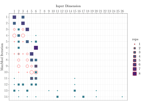
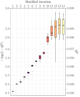
Figure 2: Model selection via the MaxMod algorithm when considering the target function in (39). The panels show: (right) the choices made by the MaxMod and (left) the boxplot of the $Q^{2}$ criterion per iteration of the algorithm. Results are shown for ten replicates of the experiment considering different LHD-based training datasets with $n=7D_{o}$ with $D_{o}=6$ the number of active input variables. In the left panel, squares represent variables that are newly selected or refined by MaxMod, while red circles represent variables that are being merged. The size and color of the markers indicate the frequency of the corresponding choice made by MaxMod over multiple iterations. In the right panel colours of the boxes correspond to the median: lighter colours correspond to higher medians.

Figure 2 shows the decisions made by the MaxMod algorithm alongside boxplots showing the $Q^{2}$ criterion per iteration for ten different replicates. In the right panel, we observe that MaxMod initially activates variables $x_{1}$ and $x_{3}$. Following their activation in the first two iterations, the algorithm then decides between merging them into a single block or activating variables $x_{2}$ and $x_{4}$. It then proceeds with options such as creating a new block with $x_{2}$ and $x_{4}$, activating and merging the remaining variables $x_{5}$ and $x_{6}$, or refining the knots of $x_{2},x_{4},x_{5}$ and $x_{6}$. As anticipated, variables $x_{1}$ and $x_{3}$ are less frequently refined. By the 12th iteration, the algorithm consistently identifies the true partition $\mathcal{P}=\{\{1,3\},\{2,4\},\{5,6\}\}$ across all ten replicates in the experiment. In the left panel, we observe the $Q^{2}$ criterion improves with each iteration, leading to a stable (median) behavior above $Q^{2}=0.995$ after twelve iterations.

Note that beyond twelve iterations, MaxMod starts considering the activation of dummy variables or refining variables $x_{1}$ and $x_{6}$, which is an undesired behavior considering the nature of the target function in (39). This behavior may be attributed to significant empirical correlations between dummy variables and active variables due to the experimental design. To mitigate this issue, adapting the stopping criterion of the algorithm to achieve convergence earlier when neither the $\mathrm{L2Mod}$ nor the $\mathrm{SMSE}$ criterion shows significant improvement would be beneficial.

For a fixed replicate, Figure 3 shows that both $\mathrm{SE}$ and $\mathrm{L2Mod}$ tend to decrease over iterations. On the 13th iteration of MaxMod, one can notice that the SMSE slightly increase. One might question why the interpolation of the predictor $\widehat{Y}^{\mathcal{S}}_{\mathcal{P}}$ on the 10th iteration is better than the one in the 11th. Indeed, $\widehat{Y}^{\mathcal{S}}_{\mathcal{P}}$ minimizes an interpolation problem in an RKHS [37]. In fact, we have an inclusion of RKHS as for the bases. Hence, it seems natural that the solution in a higher-dimensional space interpolates better the observations. However, the noise variance $\tau^{2}$ changes the nature of the optimization problem. In Appendix C, we demonstrate that increasing the dimensionality of the RKHS space can degrade the solution in terms of interpolation.

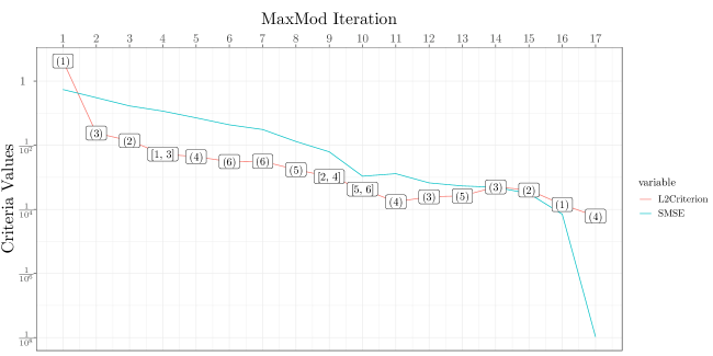
Figure 3: Evolution over MaxMod iterations of the $\mathrm{L2Mod}$ (red curve) and $\mathrm{SMSE}:=\mathrm{SE}/\sum_{i=1}^{n}(Y_{i}-\bar{Y})^{2}$ (blue curve). The choice made by the algorithm per iteration is displayed in a text box where “$(i)$” indicates the activation or the refinement of the variable $i$, while “$[i_{1},\ldots,i_{k}]$” indicates the creation of a block composed of variables $i_{1},\ldots,i_{k}$.

5.3 Real application: Coastal flooding

We examine a coastal flood application in 5D previously studied in [30, 19, 21]. The dataset is available in the R package profExtrema [38].

The application focuses on the Boucholeurs district located on the French Atlantic Coast near the city of La Rochelle. This site was hit by the Xynthia storm in February 2010, which caused the inundation of several areas and severe human and economic damage. We analyze here the flooded area ($A_{flood},[m^{2}]$) induced by overflow processes by using the hydrodynamic numerical model detailed in [39]. The dataset comprises $200$ numerical results of $A_{flood}$; each of them being related to the values of the parameters that describe the temporal evolution of the tide and the surge. The tide temporal signal is simplified and assumed to be represented by a sinusoidal signal, parameterized by the high-tide level $T$. The surge signal is modeled as a triangular function defined by four parameters: the surge peak $S$, the phase difference ($\phi$, [hours]) between surge peak and high tide, the durations of the rising ($t^{-}$, [hours]) and falling ($t^{+}$, [hours]) parts of the triangular surge signal. Figure 5 (left panel) shows a schematic representation of both signals. We refer to [30, 39] for further details on the context and the physical meaning of these variables.

We assume, as illustrated by [30], that $A_{flood}$ is non-decreasing with respect to $T$ and $S$. This assumption makes sense from the viewpoint of the flooding processes because both variables have a direct increasing influence on the offshore forcing conditions. In other words, the higher both variables, the higher the total sea level (which is given by the sum of both signals), and thus the higher the expected total flooded area (see Figure 5, left panel). Adopting the procedure used in [19], we consider as outcome $Y:=\log_{10}(A_{flood})$, and we apply the transform $\phi\mapsto(1+\cos(2\pi\phi))/2$. There, these transformations led to improvements in the $Q^{2}$ criterion.

We perform twenty replicates of the experiment using different training datasets, each comprising $35\%$ of the database (i.e., $n=70$), and evaluate the $Q^{2}$ criterion on the remaining data. We propose a bacGP with non-decreasing constraints on the input variables $T$ and $S$. To prevent overfitting and ensure stable results, we stop the MaxMod algorithm after ten iterations, noting that stability was achieved after the first eight iterations (see Figure 7). For prediction purposes, we focus solely on the predictor provided by MaxMod 1. We compare the $Q^{2}$ results to those obtained by the conditional mean of a non-additive unconstrained GP accounting only for the input variables already activated by MaxMod. We implement the latter using the R package DiceKriging [40].

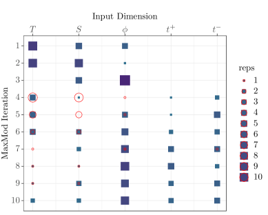
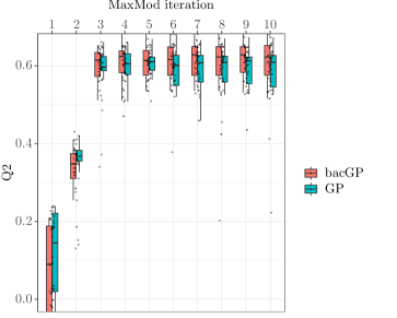
Figure 4: Model selection via the MaxMod algorithm for the coastal flooding application in 5.3. The panels show: (left) the choices made by the MaxMod and (right) the boxplot of the $Q^{2}$ criterion per iteration of the algorithm. Results are shown for twenty replicates of the experiment considering different training datasets considering 35% of the database (i.e. $n=70$). Description of the first panel is the same as in Figure 2. For the second panel, $Q^{2}$ results led by the bacGP (red) are compared to those obtained by an non-additive unconstrained GP (blue) defined on the active dimensions in the sub-partition found by MaxMod. We recall here that $\bm{x}=(T,S,\phi,t^{+},t^{-})$.

Figure 4 (left panel) illustrates the progression of the MaxMod algorithm. Initially, it activates the variables $T$, $S$, and $\phi$. By the third iteration, it focuses on refining variables $T$ and $\phi$, merging $T$ and $S$, or activating additional variables. After ten iterations, the algorithm deems all five input dimensions relevant and suggests considering interactions between $T$ and $S$.

These results can be interpreted in terms of flooding processes:

• The importance of $S$ and $T$ is physically significant since these two variables have a direct impact on the sea level at the coast, and therefore on the total amount of water that can potentially invade inland in the event of flooding.

• The mirroring role of $S$ and $T$ explains the relevance of merging them, i.e., the increase in $T$ or $S$ is interchangeable.

• The importance of $\phi$ is logical if we consider that when $\phi$ (with the transformation described above) is maximum, the two temporal signals, tide and surge, are in phase and the total amount of water is maximum.

These interpretations are consistent with a sensitive analysis (SA) using the FANOVA-decomposition in [41] and the total interaction index in [42]. The latter are estimated using a non-additive unconstrained GP (with a constant trend) trained on the entire database, and the estimator of [43] with 50k function evaluations. Consistently with our results, this experiment highlighted the relevant interaction between $S$ and $T$ and, to some extent, between $T$ and $\phi$, with a total interaction index denoted ($tii$) of the order of 20%. The interaction structure is depicted in Figure 5 (right panel).

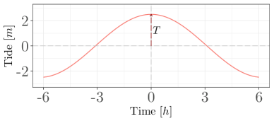
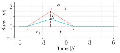
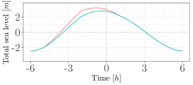
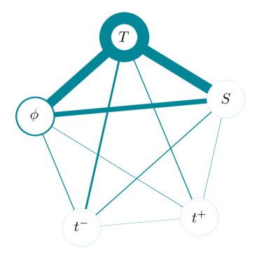
Figure 5: (left) Schematic representation of the tide (top) and surge (middle) temporal signal used in the real test case. The input variables correspond to the parameters outlined with dashed arrows. The sum of both signals results in the total sea level (bottom) which determines the offshore forcing conditions of the hydrodynamic numerical model used to simulate the flooding processes. A blue case is indicated where the surge peak $S$ is below the one of the red case resulting in a lower total sea level height. (right) FANOVA graph representing the interaction structure in the marine flooding case. The linewidth of the nodes is proportional to the Sobol first order index (main effect) and the linewidth of the graph edges proportional to the total interaction index.

We recall that the aforementioned SA was obtained using the entire database (i.e. $n=200$). Interestingly, when repeating the experiment with only 35% of the database (i.e. $n=70$), as suggested when testing the MaxMod algorithm, the interaction structure could hardly be retrieved. The total interaction indices were highly variable over 20 replicates of the experiments. For $S$ and $T$, the $tii$ ranged between from 2% to 15%, and for $T$ and $\phi$, from 7% to 23%. On the other hand, MaxMod successfully identified the interaction between $S$ and $T$ even with the limited number of samples, although detecting the interaction $T$ and $\phi$ remained challenging.

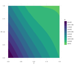
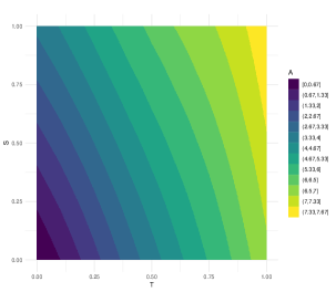
Figure 6: Bivariate representation of the functional relationship between $S$ and $T$ given $\phi=\pi$ (left panel) and $\phi=0$ (right panel) for the coastal flooding case.

In addition to the structure, the MaxMod algorithm has the practical advantage of providing the functional relationships between the three variables, which allows us to get deeper insight in their joint influence on $A_{flood}$. The analysis of Figure 6 confirms an expected behaviour from the viewpoint of flood processes. When $\phi$ gets closer to one (from panel a to e), the color of the top right hand corner of each panel changes from light green to yellow. This is in agreement with the tide and surge signals getting more and more in phase (see Figure 5 (left)), and inducing a higher total sea level offshore, hence a higher flooded area. Let us focus for instance on the combinations ($T$, $S$) for which the flooded area (log-transformed) exceeds 6. We note that the range of admissible ($T$, $S$) combinations gets wider when $\phi$ increases. This zone extends as a function of $\phi$ more rapidly (almost twice) along the $T$ direction than along the $S$ direction. This suggests that the exccedance is admissible for a more restrictive range of $S$ values, hence confirming the higher influence of $S$ (as shown in Figure 5 (right)).

Regarding the $Q^{2}$ criterion (Figure 4, right panel), the first three iterations of MaxMod are crucial for activating the most “expressive” input variables, leading to $Q^{2}>0.6$. Subsequent iterations yield slight but consistent improvements, outperforming predictions from unconstrained GPs. Similar $Q^{2}$ results have been reported in [19] for non-additive constrained GPs without MaxMod.

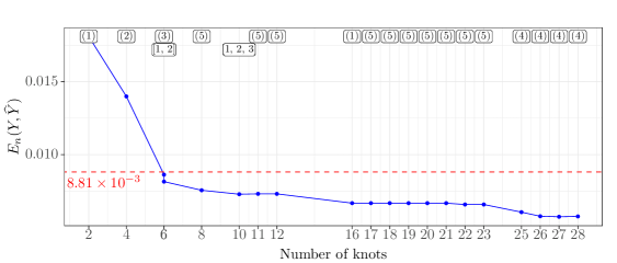
Figure 7: Evolution of the bending energy $E_{n}$ through MaxMod iterations for the bacGP. The choices of the algorithm are detailed by labels defining the same choices of those described in Figure 2. The red dashed line indicates the bending energy for the non-additive constrained GP after convergence of the MaxMod [21].

In [21], after conducting model selection of the non-additive GP via MaxMod using the entire database, their framework led to a bending energy (see definition in (37)) $E_{n}=8.81\times 10^{-3}$ for a model with $|\mathcal{L}^{\mathcal{S}}_{\mathcal{P}}|=432$ multi-dimensional knots. Here, as shown in Figure 7, similar $E_{n}$ results are obtained after three iterations of the MaxMod, requiring a smaller value of $|\mathcal{L}^{\mathcal{S}}_{\mathcal{P}}|$. After convergence, our framework achieves a value of $E_{n}(Y,\widehat{Y})=4.2\times 10^{-3}$ with $|\mathcal{L}^{\mathcal{S}}_{\mathcal{P}}|=28$. This leads to a significant computational improvement in simulation tasks, as the complexity relies on sampling a $|\mathcal{L}^{\mathcal{S}}_{\mathcal{P}}|$-dimensional truncated Gaussian vector. The improvements in terms of the $E_{n}$ are brought by the exploitation of the latent block-additive structure and the consideration of the new criterion $\mathcal{K}$ (see definition in (35)), which also seeks the minimization of the square error (i.e. the bending energy up to renormalization).

6 Conclusion

We introduced a novel block-additive constrained GP framework that allows for interactions between input variables while ensuring monotonicity constraints. As shown in the numerical experiments, the block-additive structure of the model makes it particularly well-suited for functions characterized by strong inter-variable dependencies, all while maintaining tractable computations. For model selection (i.e., the choice of the blocks), we developed the sequential MaxMod algorithm which relies on the maximization of a criterion constructed with the square norm of the modification of the MAP predictor between consecutive iterations and the square error of the predictor at the observations. MaxMod also seeks to identify the most influential input variables, making it efficient for dimension reduction. Our approach provides efficient implementations based on new theoretical results (in particular the conditions for inclusion relationships between bases composed of hat basis functions and the corresponding change-of-basis matrices) and matrix inversion properties. R codes were integrated into the open-source library lineqGPR [34].

Through various toy numerical examples, we demonstrated the framework’s scalability up to 120 dimensions and its ability to identify suitable blocks of interacting variables. We also assessed the model in a real-world 5D coastal flooding application. The derived blocks together with the block-predictors have proven to be a key for interpreting the physical processes acting during flooding. Only a limited budget of observations of the coastal flooding simulator is necessary, which is very beneficial given the high cost of this simulator, to identify the most influential factors, their interactions as well as their functional relationships. In addition, we provide open source codes to reproduce the numerical results.

The proposed work focused on applications satisfying monotonicity constraints, but it can be used to handle other types of constraints, such as componentwise convexity. We note that many applications in fields such as biology and environmental sciences require handling boundedness and positivity constraints. For the additive case, these types of constraints do not verify the equivalence in (7). Therefore, a potential future direction is to adapt the proposed framework to handle these constraints.

Additionally, theoretical guarantees of the MaxMod algorithm could be further investigated. Indeed, it would be beneficial to show as in [21] that the sequence of predictors converges to the infinite-dimensional constrained minimization solution in the RKHS induced by the kernel of the GP as developed in [31]. Moreover, except from [44], very few asymptotic results exist in the setting where the number of observations goes to infinity. It would be interesting to obtain more of these results, in particular related to the estimation of block structures.

Appendix A Proof of Proposition 1

The aim is to compute the explicit expression of the quantity in (32):

$$\left\|\widehat{Y}^{\mathcal{S}^{\star}}_{\mathcal{P}^{\star}}-\widehat{Y}^{\mathcal{S}}_{\mathcal{P}}\right\|^{2}_{L^{2}}.$$

For the sake of readability, in this proof, we simplify the notations by removing the indexes “$\mathcal{S}$” and “$\mathcal{P}$” on every object. Variables denoted with a superscript $\star$ refer to the couple $(\mathcal{P}^{\star},\mathcal{S}^{\star})$ as defined in Section 4.1. Variables without the superscript refer to the couple $(\mathcal{P},\mathcal{S})$. This leads to the following notations:

• $\widehat{Y}=\widehat{Y}^{\mathcal{S}}_{\mathcal{P}}$ (similarly, $\widehat{Y}^{\star}=\widehat{Y}^{\mathcal{S}^{\star}}_{\mathcal{P}^{\star}}$),

• $\mathcal{L}_{j}=\mathcal{L}^{\mathcal{S}}_{\mathcal{B}_{j}}$ (similarly, $\mathcal{L}^{\star}_{j}=\mathcal{L}^{\mathcal{S}^{\star}}_{\mathcal{B}_{j}^{\star}}$),

• $\widehat{Y}_{j}=\sum_{\underline{\ell}_{j}\in\mathcal{L}^{\mathcal{S}}_{\mathcal{B}_{j}}}Y_{j}(t_{\underline{\ell}_{j}})\phi_{\underline{\ell}_{j}}$ (similarly, $\widehat{Y}^{\star}_{j}=\sum_{\underline{\ell}_{j}\in\mathcal{L}^{\mathcal{S}^{\star}}_{\mathcal{B}_{j}^{\star}}}Y_{j}(t_{\underline{\ell}_{j}})\phi^{\star}_{\underline{\ell}_{j}}$),

• $\mathcal{L}=\mathcal{L}^{\mathcal{S}}_{\mathcal{P}}=\bigcup_{j=1}^{B}\mathcal{L}_{j}$ (similarly, $\mathcal{L}^{\star}=\mathcal{L}^{\mathcal{S}^{\star}}_{\mathcal{P}^{\star}}=\bigcup_{j=1}^{B^{\star}}\mathcal{L}^{\star}_{j}$).

Furthermore, to alleviate the notation, we will sometimes simply write $\phi_{\underline{\ell}_{j}}$ instead of $\phi^{s^{(j)}}_{\underline{\ell}_{j}}$, when considering a hat basis function associated to a block $j$ with subdivision $s^{(j)}$. In other words, when the ambient block and thus the ambient subdivision is fixed, we will omit the corresponding superscript. Similarly we will sometimes simply write $\phi^{\star}_{\underline{\ell}_{j}}$ instead of $\phi^{\star s^{(j)}}_{\underline{\ell}_{j}}$.

A.1 Change of basis when updating the subdivision and/or the partition

As a preliminary result, we study the change of basis of hat functions associated to two different pairs of blocks and subdivisions $(\mathcal{S},\mathcal{P})$ and $(\mathcal{S}^{\star},\mathcal{P}^{\star})$. These changes of basis functions extend to several blocks of variables the results presented in [21, Section SM2]. Roughly speaking, an important idea is that a one-dimensional piecewise affine function $f$ defined on a subdivision remains piecewise affine when defined on a finer subdivision. Furthermore, to express $f$ with the hat basis functions of the finer subdivision, it is sufficient to consider the values of $f$ on its knots.

Lemma 1 (Expression of the elements of $\beta^{\mathcal{S}}_{\mathcal{P}}$ in $\beta^{\mathcal{S}^{\star}}_{\mathcal{P}^{\star}}$).

Recall $\mathcal{S}=(s^{(1)},\ldots,\,s^{(D)})$ and $\mathcal{P}=\{\mathcal{B}_{1},\ldots,\mathcal{B}_{B}\}$. We have the following explicit expressions of the basis functions in $\beta^{\mathcal{S}}_{\mathcal{P}}$ in the new basis $\beta^{\mathcal{S}^{\star}}_{\mathcal{P}^{\star}}$ for every choice of MaxMod introduced in Section 4.1:

Activate

Let $i_{0}$ be the index of the activated variable. Recall that this variable forms a new block. Thus $\mathcal{P}^{\star}=\{\mathcal{B}_{1},\cdots,\mathcal{B}_{B},\{i_{0}\}\}$ and $\beta^{\mathcal{S}^{\star}}_{\mathcal{P}^{\star}}$ is the set of functions

$$\beta^{\mathcal{S}^{\star}}_{\mathcal{P}^{\star}}=\beta^{\mathcal{S}}_{\mathcal{P}}\cup\beta^{\mathcal{S}^{\star}}_{\{i_{0}\}},$$

where $\beta^{\mathcal{S}^{\star}}_{\{i_{0}\}}=\{\bm{x}\mapsto\widehat{\phi}_{-1,0,1}(x_{i_{0}}),\bm{x}\mapsto\widehat{\phi}_{0,1,2}(x_{i_{0}})\}$. Hence, every function in $\beta^{\mathcal{S}}_{\mathcal{P}}$ lies in $\beta^{\mathcal{S}^{\star}}_{\mathcal{P}^{\star}}$.

Refine

Let $s^{(i_{0})}$ be the refined subdivision in the block $\mathcal{B}_{j_{0}}$. Write $p^{\star}$ for the index of the left-nearest neighbor knot to $t^{\star}$ in the subdivision $s^{(i_{0})}$: $t^{(i_{0})}_{p^{\star}}<t^{\star}<t^{(i_{0})}_{p^{\star}+1}$. For any $j\neq j_{0}$, the elements $\phi_{\underline{\ell}_{j}}$ of $\beta^{\mathcal{S}}_{\mathcal{B}_{j}}$ are already in $\beta^{\mathcal{S}^{\star}}_{\mathcal{P}^{\star}}$. Consider a multi-index $\underline{\ell}_{j_{0}}=(\ell_{1},...,\ell_{|\mathcal{B}_{j_{0}}|})\in\mathcal{L}^{\mathcal{S}}_{\mathcal{B}_{j_{0}}}$. Without loss of generality we assume that the variable $i_{0}$ is the first in the block $\mathcal{B}_{j_{0}}$, with corresponding knots indexed by $\ell_{1}$ in $\underline{\ell}_{j_{0}}$. Let $\delta_{i_{0}}=(1,0,\ldots,0)\in\mathbb{R}^{|\mathcal{B}_{j_{0}}|}$. If $\ell_{1}\not\in\{p^{\star},p^{\star}+1\}$ then $\phi_{\underline{\ell}_{j_{0}}}\in\beta^{\mathcal{S}^{\star}}_{\mathcal{P}^{\star}}$. If $\ell_{1}=p^{\star}$ then

$$\phi_{p^{\star}}=\phi^{\star}_{p^{\star}}+\phi_{p^{\star}}(t^{\star})\phi^{\star}_{p^{\star}+1},$$

which can be checked by computing the values at the knots of the finest subdivision $s^{\star(i_{0})}$ (of indices $p^{\star}$ and $p^{\star}+1$). Similarly if $\ell_{1}=p^{\star}+1$, then $\phi_{p^{\star}+1}=\phi_{p^{\star}+1}(t^{\star})\phi^{\star}_{p^{\star}+1}+\phi^{\star}_{p^{\star}+2}$. Finally for these two latter cases, we deduce, by tensorization,

$$\phi_{\underline{\ell}_{j_{0}}}=\begin{cases}\phi^{\star}_{\underline{\ell}_{j_{0}}}+\phi_{p^{\star}}(t^{\star})\phi^{\star}_{\underline{\ell}_{j_{0}}+\delta_{i_{0}}}&~{}\mbox{if}~{}\ell_{1}=p^{\star}\\ \phi_{p^{\star}+1}(t^{\star})\phi^{\star}_{\underline{\ell}_{j_{0}}}+\phi^{\star}_{\underline{\ell}_{j_{0}}+\delta_{i_{0}}}&~{}\mbox{if}~{}\ell_{1}=p^{\star}+1.\end{cases}$$

Merge

In the case where we merge two blocks, suppose without loss of generality that $\mathcal{B}_{1}$ and $\mathcal{B}_{2}$ are merged, so that $\mathcal{B}^{\star}_{1}=\mathcal{B}_{1}\cup\mathcal{B}_{2}$. For $j=1,2$, let $\mathcal{B}_{j}=\{i_{j,1},i_{j,2},\ldots,i_{j,{|\mathcal{B}_{j}|}}\}$ with $i_{j,1}<\cdots<i_{j,{|\mathcal{B}_{j}|}}$. Then suppose that the elements in $\mathcal{B}^{\star}_{1}$ are ordered as $\mathcal{B}^{\star}_{1}=\{i_{1,1},\ldots,i_{1,{|\mathcal{B}_{1}|}},i_{2,1},\ldots,i_{2,{|\mathcal{B}_{2}|}}\}$. For any $j>2$, the basis functions $\phi_{\underline{\ell}_{j}}\in\beta^{\mathcal{S}}_{\mathcal{B}_{j}}$ are in $\beta^{\mathcal{S}^{\star}}_{\mathcal{P}^{\star}}$, since the block $\mathcal{B}_{j}$ is not modified by the merge. Now, consider $\underline{\ell}_{1}=(\ell_{1},...,\ell_{|\mathcal{B}_{1}|})\in\mathcal{L}^{\mathcal{S}}_{\mathcal{B}_{1}}$. Using that the hat basis functions corresponding to a block sum to one, the following equality holds:

$$\phi_{\underline{\ell}_{1}}(\bm{x}) = \left(\prod_{a=1}^{|\mathcal{B}_{1}|}\phi_{\ell_{a}}^{(s^{(i_{1,a})})}(x_{i_{1,a}})\right)\cdot 1$$

$$= \left(\prod_{a=1}^{|\mathcal{B}_{1}|}\phi_{\ell_{a}}^{(s^{(i_{1,a})})}(x_{i_{1,a}})\right)\cdot\left(\sum_{\underline{\ell}_{2}\in\mathcal{L}^{\mathcal{S}}_{\mathcal{B}_{2}}}\phi_{\underline{\ell}_{2}}^{(\mathcal{B}_{2})}(x_{\underline{\ell}_{2}})\right)=\sum_{\underline{\ell}^{\star}\in\mathcal{L}^{\star}_{\underline{\ell}_{1}}}\phi^{\star}_{\underline{\ell}^{\star}}(\bm{x}),$$

with $\mathcal{L}^{\star}_{\underline{\ell}_{1}}:=\{(\ell^{\star}_{1},\ldots,\ell^{\star}_{|\mathcal{B}_{1}|+|\mathcal{B}_{2}|})\in\mathcal{L}^{\mathcal{S}}_{\mathcal{P}^{\star}},(\ell^{\star}_{1},\ldots,\ell^{\star}_{|\mathcal{B}_{1}|})=\underline{\ell}_{1}\}$. Similarly, for $\phi_{\underline{\ell}_{2}}\in\beta^{\mathcal{S}}_{\mathcal{B}_{2}}$,

$$\phi_{\underline{\ell}_{2}}=\sum_{\underline{\ell}^{\star}\in\mathcal{L}^{\star}_{\underline{\ell}_{2}}}\phi^{\star}_{\underline{\ell}^{\star}},$$

where $\mathcal{L}^{\star}_{\underline{\ell}_{2}}:=\{(\ell^{\star}_{1},\ldots,\ell^{\star}_{|\mathcal{B}_{1}|+|\mathcal{B}_{2}|})\in\mathcal{L}^{\mathcal{S}}_{\mathcal{P}^{\star}},(\ell^{\star}_{|\mathcal{B}_{1}|+1},\ldots,\ell^{\star}_{|\mathcal{B}_{1}|+|\mathcal{B}_{2}|})=\underline{\ell}_{2}\}$.

Corollary 1.

From Lemma 1, a linear combination of the former basis functions from $(\mathcal{S},\mathcal{P})$ is also a linear combination of the new basis functions from $(\mathcal{S}^{\star},\mathcal{P}^{\star})$. Formally, for every vector $\widehat{\bm{\xi}}\in\mathbb{R}^{|\mathcal{L}|}$ there exists a vector $\widehat{\bm{\xi}}^{\prime}$ in $\mathbb{R}^{|\mathcal{L}^{\star}|}$, obtained by the change of basis formula, such that

$$\bm{\Phi}^{\top}\widehat{\bm{\xi}}=\bm{\Phi}^{\star\top}\widehat{\bm{\xi}}^{\prime},$$

where $\bm{\Phi}$ (respectively $\bm{\Phi}^{\star}$) are the vector functions introduced in (23) for the sub-partition $\mathcal{P}$ (respectively $\mathcal{P}^{\star}$) and subdivision $\mathcal{S}$ (respectively $\mathcal{S}^{\star}$).

A.2 Computation of the L2Mod criterion

Since our model is block additive, we have $\big{(}\widehat{Y}^{\star}-\widehat{Y}\big{)}^{2}=\left(\sum_{j=1}^{B}\left[\widehat{Y}_{j}-\widehat{Y}^{\star}_{j}\right]\right)^{2}$. By expanding the square and integrating, we deduce:

$$\left\|\widehat{Y}^{\star}-\widehat{Y}\right\|^{2}_{L^{2}}=\underbrace{\sum_{j=1}^{B}\int_{[0,1]^{\mathcal{B}^{\star}_{j}}}\big{(}\widehat{Y}_{j}-\widehat{Y}^{\star}_{j}\big{)}^{2}\,d\lambda}_{S_{1}}+2\underbrace{\sum_{1\leq i<j\leq B}\Big{(}\int_{[0,1]^{\mathcal{B}^{\star}_{i}}}(\widehat{Y}_{i}-\widehat{Y}^{\star}_{i})\,d\lambda\Big{)}\Big{(}\int_{[0,1]^{\mathcal{B}^{\star}_{j}}}(\widehat{Y}_{j}-\widehat{Y}^{\star}_{j})\,d\lambda\Big{)}}_{S_{2}},$$ (40)

where $d\lambda$ is Lebesgue measure in the appropriate dimension. In $S_{2}$, we have exploited that the blocks are disjoint to write integrals of products as products of integrals. We will now investigate both sums $S_{1}$ and $S_{2}$ of (40) separately. Our approach for computing these two sums is to express $\widehat{Y}_{i}$ and $\widehat{Y}^{\star}_{i}$ in the “finest” basis corresponding to $\widehat{Y}^{\star}_{i}$ and to use the change of basis formulas of Lemma 1.

A.2.1 Computation of $\mathbf{S_{1}}$

From Corollary 1, we can consider the vector $\widehat{\bm{\xi}}^{\prime}$, which satisfies $\bm{\Phi}^{\top}\widehat{\bm{\xi}}=\bm{\Phi}^{\star\top}\widehat{\bm{\xi}}^{\prime}$. Note that from (31), $\widehat{Y}(\bm{x})=\bm{\Phi}^{\top}(\bm{x})\widehat{\bm{\xi}}$ and $\widehat{Y}^{\star}(\bm{x})=\bm{\Phi}^{\star\top}(\bm{x})\widehat{\bm{\xi}}^{\prime}$. We can now rewrite the expression as follows

$$\int_{[0,1]^{\mathcal{B}^{\star}_{j}}}(\widehat{Y}_{j}-\widehat{Y}^{\star}_{j})^{2}\,d\lambda=\int_{[0,1]^{\mathcal{B}^{\star}_{j}}}\Big{(}\sum_{\underline{\ell}_{j}\in\mathcal{L}^{\star}_{j}}(\widehat{\bm{\xi}}^{\prime}_{j,\underline{\ell}_{j}}-\widehat{\bm{\xi}}^{\star}_{j,\underline{\ell}_{j}})\phi^{\star}_{j,\underline{\ell}_{j}}\Big{)}^{2}d\lambda=\sum_{\underline{\ell}_{j},\underline{\ell}^{\prime}_{j}\in\mathcal{L}^{\star}_{j}}(\widehat{\bm{\xi}}^{\prime}_{j,\underline{\ell}_{j}}-\widehat{\bm{\xi}}^{\star}_{j,\underline{\ell}_{j}})(\widehat{\bm{\xi}}^{\prime}_{j,\underline{\ell}^{\prime}_{j}}-\widehat{\bm{\xi}}^{\star}_{j,\underline{\ell}^{\prime}_{j}})\int_{[0,1]^{\mathcal{B}^{\star}_{j}}}\phi^{\star}_{\underline{\ell}_{j}}\phi^{\star}_{\underline{\ell}^{\prime}_{j}}\,d\lambda.$$

Now, we define the $|\mathcal{L}^{\star}|$-dimensional vector $\bm{\eta}$ as

$$\bm{\eta}=(\bm{\eta}_{j,\underline{\ell}_{j}})_{1\leq j\leq B,\underline{\ell}_{j}\in\mathcal{L}^{\star}_{j}},\hskip 28.45274pt\bm{\eta}_{j,\underline{\ell}_{j}}=(\widehat{\bm{\xi}}^{\prime}_{j,\underline{\ell}_{j}}-\widehat{\bm{\xi}}^{\star}_{j,\underline{\ell}_{j}}),$$ (41)

and the $|\mathcal{L}^{\star}_{j}|$-dimensional matrix $\bm{\Psi}^{j}$ as follows

$$\bm{\Psi}^{j}_{\underline{\ell}_{j},\underline{\ell}^{\prime}_{j}}=\int_{[0,1]^{\mathcal{B}^{\star}_{j}}}\phi^{\star}_{\underline{\ell}_{j}}\phi^{\star}_{\underline{\ell}^{\prime}_{j}}d\lambda=\prod_{i\in\mathcal{B}^{\star}_{j}}\int_{0}^{1}\widehat{\phi}^{\star(i)}_{{\underline{\ell}_{j,i}}}\phi^{\star(i)}_{{\underline{\ell}^{\prime}_{j,i}}}\,d\lambda=\prod_{i\in\mathcal{B}^{\star}_{j}}\Psi^{(i)}_{\underline{\ell}_{j,i},\underline{\ell}^{\prime}_{j,i}},$$ (42)

with

$$\Psi^{(i)}_{\underline{\ell}_{j,i},\underline{\ell}^{\prime}_{j,i}}=\begin{cases}\dfrac{t^{(i)}_{\underline{\ell}_{j,i}+1}-t^{(i)}_{\underline{\ell}_{j,i}}}{3}&\text{if }\underline{\ell}_{j,i}=\underline{\ell}^{\prime}_{j,i}=1,\\ \dfrac{t^{(i)}_{\underline{\ell}_{j,i}+1}-t^{(i)}_{\underline{\ell}_{j,i}-1}}{3}&\text{if }2\leq\underline{\ell}_{j,i}=\underline{\ell}^{\prime}_{j,i}\leq m^{(i)}-1,\\ \dfrac{t^{(i)}_{\underline{\ell}_{j,k}}-t^{(i)}_{\underline{\ell}_{j,i}-1}}{3}&\text{if }\underline{\ell}_{j,i}=\underline{\ell}^{\prime}_{j,i}=m^{(i)},\\ \dfrac{\big{|}t^{(i)}_{\underline{\ell}_{j,i}}-t^{(i)}_{\underline{\ell}^{\prime}_{j,i}}\big{|}}{6}&\text{if }|\underline{\ell}_{j,i}-\underline{\ell}^{\prime}_{j,i}|=1,\\ 0&\text{if }|\underline{\ell}_{j,i}-\underline{\ell}^{\prime}_{j,i}|>1.\end{cases}$$ (43)

The expressions in (43) correspond to the Gram matrices of univariate hat basis functions and can be found for instance in [21]. We finally get the result,

$$S_{1}=\sum_{j=1}^{B}\int_{[0,1]^{\mathcal{B}_{j}}}(\widehat{Y}_{j}-\widehat{Y}^{\star}_{j})^{2}\,d\lambda=\sum_{j=1}^{B}\sum_{\underline{\ell}_{j},\underline{\ell}^{\prime}_{j}\in\mathcal{L}^{\star}_{j}}\bm{\eta}_{j,\underline{\ell}_{j}}\bm{\eta}_{j,\underline{\ell}^{\prime}_{j}}\bm{\Psi}^{j}_{\underline{\ell}_{j},\underline{\ell}^{\prime}_{j}}=\bm{\eta}^{\top}\bm{\Psi}\bm{\eta},$$ (44)

writing $\bm{\Psi}$ as the $|\mathcal{L}^{\star}|$-dimensional matrix and $\bm{\eta}$ as the $|\mathcal{L}^{\star}|$-dimensional vector

$$\bm{\Psi}=\bNiceArray{ccc}[margin]\bm{\Psi}^{1}&\Block{2-2}{0}\\ \Block{2-2}{0}\ddots\\ \bm{\Psi}^{B},\hskip 28.45274pt\bm{\eta}=\bNiceArray{c}[margin]\bm{\xi}^{\prime}_{1}-\bm{\xi}_{1}\\ \vdots\\ \bm{\xi}^{\prime}_{B}-\bm{\xi}_{B}.$$ (45)

Remark 5.

The computational cost of $S_{1}$ in (44) is linear with respect to the dimension $|\mathcal{L}^{\star}|$. Indeed, for each $\underline{\ell}_{j}\in\mathcal{L}^{\star}_{j}$, there are at most $3^{|\mathcal{B}^{\star}_{j}|}$ multi-indices $\underline{\ell}^{\prime}_{j}\in\mathcal{L}^{\star}_{j}$ such that $\bm{\Psi}^{j}_{\underline{\ell},\underline{\ell}^{\prime}}\neq 0$. This is because, from Equations (42) and (43), for $\underline{\ell}_{j}\in\mathcal{L}^{\star}_{j}$ , it is easy to see that $\bm{\Psi}^{j}_{\underline{\ell}_{j},\underline{\ell}^{\prime}_{j}}\neq 0$ implies that $||\underline{\ell}_{j}-\underline{\ell}_{j}^{\prime}||_{\infty}\leq 1$. Since $\underline{\ell}_{j}$ and $\underline{\ell}^{\prime}_{j}$ both lie in $\mathbb{Z}^{|\mathcal{B}^{\star}_{j}|}$, the number of values that $\underline{\ell}^{\prime}_{j}$ can take such that $\bm{\Psi}^{j}_{\underline{\ell}_{j},\underline{\ell}^{\prime}_{j}}\neq 0$ is bounded by $3^{|\mathcal{B}^{\star}_{j}|}$. Hence, the number of non-zero terms in $\displaystyle{\sum_{\underline{\ell}_{j},\underline{\ell}^{\prime}_{j}\in\mathcal{L}^{\star}_{j}}\bm{\eta}_{j,\underline{\ell}_{j}}\bm{\eta}_{j,\underline{\ell}^{\prime}_{j}}\bm{\Psi}^{j}_{\underline{\ell}_{j},\underline{\ell}^{\prime}_{j}}}$ in (44) is bounded by $|\mathcal{L}^{\star}_{j}|3^{|\mathcal{B}^{\star}_{j}|}$.

A.2.2 Computation of $\mathbf{S_{2}}$

We define the $|\mathcal{L}^{\star}|$-dimensional vector $\bm{E}$,

$$\bm{E}\in\mathbb{R}^{|\mathcal{L}^{\star}|},\hskip 28.45274pt\bm{E}=(\bm{E}_{j,\underline{\ell}_{j}})_{1\leq j\leq B,\,\underline{\ell}_{j}\in\mathcal{L}^{\star}_{j}},$$ (46)

with

$$\bm{E}_{\underline{\ell}_{j}}=\int_{[0,1]^{\mathcal{B}^{\star}_{j}}}\phi^{\star}_{\underline{\ell}_{j}}\,d\lambda=\int_{[0,1]^{\mathcal{B}^{\star}_{j}}}\prod_{i\in\mathcal{B}_{j}}\phi^{s^{\star(i)}}_{\underline{\ell}_{j,i}}\,d\lambda=\prod_{i\in\mathcal{B}^{\star}_{j}}\bm{E}_{j,\underline{\ell}_{j,i}},$$ (47)

and $\bm{E}_{j,\underline{\ell}_{j,i}}=\int_{0}^{1}\phi^{s^{\star(i)}}_{\underline{\ell}_{j,i}}\,d\lambda$. Then we can easily compute (see for instance [21])

$$\bm{E}_{j,\underline{\ell}_{j,i}}=\begin{cases}\frac{1}{2}(t^{(i)}_{\underline{\ell}_{j,i}+1}-t^{(i)}_{\underline{\ell}_{j,i}})&\text{if }\underline{\ell}_{j,i}=1,\\ \frac{1}{2}(t^{(i)}_{\underline{\ell}_{j,i}+1}-t^{(i)}_{\underline{\ell}_{j,i}-1})&\text{if }2\leq\underline{\ell}_{j,i}\leq m^{\star(i)}-1,\\ \frac{1}{2}(t^{(i)}_{\underline{\ell}_{j,i}}-t^{(i)}_{\underline{\ell}_{j,i}-1})&\text{if }\underline{\ell}_{j,i}=m^{\star(i)}.\end{cases}$$ (48)

Then, taking $\widehat{\bm{\xi}}^{\prime}$ from Corollary 1 we can write,

$$\rho_{j}:=\int_{[0,1]^{\mathcal{B}^{\star}_{j}}}(\widehat{Y}_{j}-\widehat{Y}^{\star}_{j})\,d\lambda=\int_{[0,1]^{\mathcal{B}^{\star}_{j}}}\sum_{\underline{\ell}_{j}\in\mathcal{L}^{\star}_{j}}\phi^{\star}_{\underline{\ell}_{j}}\big{(}\widehat{\bm{\xi}}^{\prime}_{j,\underline{\ell}_{j}}-\widehat{\bm{\xi}}^{\star}_{j,\underline{\ell}_{j}}\big{)}\,d\lambda=\sum_{\underline{\ell}_{j}\in\mathcal{L}^{\star}_{j}}\bm{\eta}_{j,\underline{\ell}_{j}}\bm{E}_{\underline{\ell}_{j}}=\bm{\eta}_{j}^{\top}\bm{E}_{j}.$$

This gives

$$S_{2}=2\sum_{1\leq i<j\leq B}\rho_{i}\rho_{j}=\left(\sum_{i=1}^{B}\rho_{i}\right)^{2}-\sum_{i=1}^{B}\rho_{i}^{2}=(\bm{\eta}^{\top}\bm{E})^{2}-\sum_{1\leq j\leq B}\left(\bm{\eta}_{j}^{\top}\bm{E}_{j}\right)^{2}.$$

This gives an expression of $S_{2}$ that has a linear computational cost with respect to $B$. Gathering the expressions of $S_{1}$ and $S_{2}$, together with (40) concludes the proof of Proposition 1.

Appendix B Kernel hyperparameters estimation

Here we consider a fixed partition $\mathcal{P}=\{\mathcal{B}_{1},\ldots,\mathcal{B}_{B}\}$ and fixed subdivisions $\mathcal{S}=\{s^{(1)},\ldots,s^{(B)}\}$. We keep notations $X^{(i)},X^{\mathcal{B}_{j}},X$ introduced in Section 2. We consider a parametric family of covariance functions for the block-additive model (3), given by (11). Within each block, we choose to tensorize univariate covariance functions. Formally, we let

$$k_{\mathcal{P},\theta}(\bm{x},\bm{x}^{\prime})=\sum_{j=1}^{B}\prod_{i\in\mathcal{B}_{j}}k_{\theta^{(i)}}(x_{i},x^{\prime}_{i}),$$

for $\bm{x},\bm{x}^{\prime}\in X$ and $\theta=(\theta^{(1)},\ldots,\theta^{(D)})$, where for each $i$, $k_{\theta^{(i)}}$ is a covariance function on $X^{(i)}\times X^{(i)}$ and $\Theta^{(i)}\subseteq\mathbb{R}^{q_{i}}$ for some $q_{i}\in\mathbb{N}$.

Then, we consider standard maximum likelihood estimation for the finite-dimensional GP $\widetilde{Y}^{\mathcal{S}}_{\mathcal{P}}$ in (24) with noisy observations, see [17]. Formally we consider the finite-dimensional covariance function in (21) that yields the finite-dimensional covariance matrix $\bm{K}_{\theta}=\bm{\Phi}(\bm{X})^{\top}\widetilde{k}_{\theta}(\bm{X},\bm{X})\bm{\Phi}(\bm{X})$ of $\widetilde{Y}^{\mathcal{S}}_{\mathcal{P}}(\bm{X})$. The noisy observation vector $\bm{Y}=\widetilde{Y}^{\mathcal{S}}_{\mathcal{P}}(\bm{X})+\bm{\epsilon}$ is Gaussian $\mathcal{N}(\bm{0},\bm{K}_{\theta}+\tau^{2}\bm{I}_{n})$ and the associated likelihood is given by

$$L(\theta,\tau;\bm{Y})=\frac{1}{(2\pi)^{n/2}|\bm{K}_{\theta}+\tau^{2}\bm{I}_{n}|^{1/2}}\exp\left(-\frac{1}{2}\bm{Y}^{\top}(\bm{K}_{\theta}+\tau^{2}\bm{I}_{n})^{-1}\bm{Y}\right).$$ (49)

Numerical improvements can be used for computing the inverse and determinant of $\bm{K}_{\theta}+\tau^{2}\bm{I}_{n}$, using the techniques of Section 3.3. Maximizing the likelihood over $(\theta,\tau)$ is equivalent to solving the optimization problem:

$$\underset{\begin{subarray}{c}\theta\in\Theta\\ \tau\in(0,\infty)\end{subarray}}{\mathrm{argmin}}~{}~{}\log(|\bm{K}_{\theta}+\tau^{2}\bm{I}_{n}|)+\bm{Y}^{\top}(\bm{K}_{\theta}+\tau^{2}\bm{I}_{n})^{-1}\bm{Y}.$$

To facilitate its numerical resolution, we can provide the gradient which is given explicitly, see for instance [1] [Chap 5.4]:

$$\frac{\partial L(\theta,\tau;\bm{Y})}{\partial\theta_{j,\ell}}=-\bm{Y}^{\top}(\bm{K}_{\theta}+\tau^{2}\bm{I}_{n})^{-1}\frac{\partial\bm{K}_{\theta}}{\partial\theta_{j,\ell}}(\bm{K}_{\theta}+\tau^{2}\bm{I}_{n})^{-1}\bm{Y}+\mathrm{Tr}\left((\bm{K}_{\theta}+\tau^{2}\bm{I}_{n})^{-1}\frac{\partial\bm{K}_{\theta}}{\partial\theta_{j,\ell}}\right),$$ (50)

and

$$\frac{\partial L(\theta,\tau;\bm{Y})}{\partial\tau^{2}}=\bm{Y}^{\top}(\bm{K}_{\theta}+\tau^{2}\bm{I}_{n})^{-2}\bm{Y}+\mathrm{Tr}\left((\bm{K}_{\theta}+\tau^{2}\bm{I}_{n})^{-1}\right),$$ (51)

where for $j=1,\ldots,D$, $\theta_{j,1},\ldots,\theta_{j,q_{j}}$ are the components of $\theta_{j}$.

Appendix C Evolution of the square norm over iterations

Figure 3 suggests that the MSE score can occasionally increase over some of the MaxMod iterations. Here we will show that this behavior is not caused by numerical issues, by providing theoretical examples where it occurs. We will provide these theoretical examples in the unconstrained case, for simplicity, relying on the explicit expression of the mode in this case, which coincides with the usual conditional mean of GPs.

Let $X=[0,1]$. Consider two finite vector subspaces $E_{1}$ and $E_{2}$ of $\mathcal{C}^{0}(X,\mathbb{R})$ the realisation space of our GP $\{Y(x),\,x\in X\}$, satisfying $E_{1}\subset E_{2}$. Suppose as well that $Y$ has centered and kernel $k$. We have two projections $P_{1}:\mathcal{C}^{0}(X,\mathbb{R})\to E_{1}$ and $P_{2}:\mathcal{C}^{0}(X,\mathbb{R})\to E_{2}$ such that $P_{1}\circ P_{2}=P_{1}$. We now set the two GPs $\widetilde{Y}_{1}=P_{1}(Y)$ and $\widetilde{Y}_{2}=P_{2}(Y)$. We set our observations to be $(\bm{X},\bm{Y})$. One may think that the function $\widehat{f}_{2}(\cdot)=E(\widetilde{Y}_{2}(\cdot)|\widetilde{Y}_{2}(\bm{X})+\epsilon=\bm{Y})$ better interpolates the observations $\bm{Y}$ than the function $\widehat{f}_{1}(\cdot)=E(\widetilde{Y}_{1}(\cdot)|\widetilde{Y}_{1}(\bm{X})+\epsilon=\bm{Y})$ ($\epsilon$ being a Gaussian white noise of variance $\tau^{2}$). Indeed, $\widetilde{Y}_{2}$ lives in a larger vector space than $\widetilde{Y}_{1}$. However, as already mentioned, Figure 3 shows some occasional increments of the square norm from $\widetilde{Y}_{1}$ to $\widetilde{Y}_{2}$. To interpret these increments, it is convenient to recall that for $i=1,2$ the conditional mean function $\widehat{f}_{i}$ can also be defined as the solution of a minimization problem in the RKHS $\mathcal{H}_{i}$ with kernel $\widetilde{k}_{i}$:

$$\widehat{f}_{i}=\underset{f\in\mathcal{H}_{i}}{\mathrm{argmin}}\left\|f(\bm{X})-\bm{Y}\right\|^{2}+\tau^{2}\left\|f\right\|^{2}_{\mathcal{H}_{i}}.$$ (52)

Here $\widetilde{k}_{i}$ is the (finite-dimensional) kernel of $\widetilde{Y}_{i}$. Notice that $\mathcal{H}_{1}\subseteq\mathcal{H}_{2}$ since $E_{1}\subseteq E_{2}$. Hence, we have

$$\underset{f\in\mathcal{H}_{2}}{\min}\left\|f(\bm{X})-\bm{Y}\right\|^{2}\leq\underset{f\in\mathcal{H}_{1}}{\min}\left\|f(\bm{X})-\bm{Y}\right\|^{2}.$$

However, due to the second term in (52), we can have

$$||\widehat{f}_{1}(\bm{X})-\bm{Y}||^{2}<||\widehat{f}_{2}(\bm{X})-\bm{Y}||^{2}.$$ (53)

We now give an explicit example where this happens. We will find two hat basis $\beta_{1}$ and $\beta_{2}$ such that $E_{1}=\operatorname{span}\beta_{1}\subset E_{2}=\operatorname{span}\beta_{2}$ and such that (53) holds.

Note that Section 3.3 provides an explicit expression of the function $\widehat{f}_{i}$ and thus we have

$$\left\|\widehat{f}_{i}(\bm{X})-\bm{Y}\right\|^{2}=\left\|\left(\widetilde{k}_{i}(\bm{X},\bm{X})\Big{[}\widetilde{k}_{i}(\bm{X},\bm{X})+\tau^{2}\bm{I}_{n}\Big{]}^{-1}-I_{n}\right)\bm{Y}\right\|^{2}.$$

To obtain that construction, we will first show a useful lemma.

Lemma 2.

Let $\bm{A}$ and $\bm{B}$ be two symmetric $n\times n$ matrices. If the matrix $\bm{B}-\bm{A}$ has one strictly positive eigenvalue $\lambda$ with an associated unit eigenvector $\bm{e}_{\lambda}$, then:

$$\left\|(\bm{A}[\bm{A}+\gamma\bm{I}_{n}]^{-1}-\bm{I}_{n})\bm{e}_{\lambda}\right\|>\left\|(\bm{B}[\bm{B}+\gamma\bm{I}_{n}]^{-1}-\bm{I}_{n})\bm{e}_{\lambda}\right\|$$

holds when $\gamma$ is large enough.

Proof.

We can rewrite $(\bm{A}+\gamma\bm{I}_{n})^{-1}=\gamma^{-1}(\bm{I}_{n}+\frac{\bm{A}}{\gamma})^{-1}$. Then, as $\gamma\to\infty$,

$$\left(\bm{A}+\gamma\bm{I}_{n}\right)^{-1}=\gamma^{-1}\left(\bm{I}_{n}-\frac{\bm{A}}{\gamma}+o\left(\frac{1}{\gamma}\right)\right),$$

and again

$$\bm{I}_{n}-\bm{A}(\bm{A}+\gamma\bm{I}_{n})^{-1}=\bm{I}_{n}-\frac{\bm{A}}{\gamma}+o\left(\frac{1}{\gamma}\right).$$

Note that we can have the same expression for $B$. Then, as $\gamma\to\infty$,

$$\left\|\left(\bm{I}_{n}-\frac{\bm{A}}{\gamma}+o\left(\frac{1}{\gamma}\right)\right)\bm{e}_{\lambda}\right\|^{2}>\left\|\left(\bm{I}_{n}-\frac{\bm{B}}{\gamma}+o\left(\frac{1}{\gamma}\right)\right)\bm{e}_{\lambda}\right\|^{2}.$$

The difference of the two expressions is written

$$\left\|\left(\bm{I}_{n}-\frac{\bm{A}}{\gamma}+o\left(\frac{1}{\gamma}\right)\right)\bm{e}_{\lambda}\right\|^{2}-\left\|\left(\bm{I}_{n}-\frac{\bm{B}}{\gamma}+o\left(\frac{1}{\gamma}\right)\right)\bm{e}_{\lambda}\right\|^{2}=\frac{2}{\gamma}\langle\bm{e}_{\lambda},(\bm{B}-\bm{A})\bm{e}_{\lambda}\rangle+o(\gamma^{-1})=\frac{2\lambda}{\gamma}+o(\gamma^{-1}).$$

The result follows. ∎

We do now have a way of constructing our inequality. Taking $\beta_{1}=(\phi_{1})=(\widehat{\phi}_{0,0.5,1})$ and $\beta_{2}=(\phi^{\prime}_{1},\phi^{\prime}_{2})=(\widehat{\phi}_{0,0.5,0.5+\epsilon},\widehat{\phi}_{0.5,0.5+\epsilon,1})$, we have $\phi_{1}=\phi^{\prime}_{1}+(1-2\epsilon)\phi^{\prime}_{2}$. Indeed, since $\phi_{1},\phi^{\prime}_{1},\phi^{\prime}_{2}$ are piecewise linear vanishing at $0,1$ it is sufficient to check the equality at the knots $0.5$ and $0.5+\epsilon$. In particular, we can express $\phi_{1}$ in the basis $\beta_{2}$ and thus $E_{1}\subseteq E_{2}$. Then, taking $\bm{X}=(x_{1},x_{2})=(0.5,0.5+\epsilon)$ gives

$$\Phi_{2}(\bm{X})^{\top}=\bNiceArray{cc}[margin]\phi^{\prime}_{1}(x_{1})&\phi^{\prime}_{2}(x_{1})\\ \phi^{\prime}_{1}(x_{2})\phi^{\prime}_{2}(x_{2})=I_{2}.$$

From what we said

$$\Phi_{1}(\bm{X})^{\top}=\bNiceArray{c}[margin]\phi_{1}(x_{1})\\ \phi_{1}(x_{2})=\bNiceArray{c}[margin]\phi^{\prime}_{1}(x_{1})+(1-2\epsilon)\phi^{\prime}_{2}(x_{1})\\ \phi^{\prime}_{1}(x_{2})+(1-2\epsilon)\phi^{\prime}_{2}(x_{2})\\ =\bNiceArray{c}[margin]1\\ 1-2\epsilon\\ .$$

We can then express $\widetilde{k}_{1}(\bm{X},\bm{X})$:

$$\widetilde{k}_{1}(\bm{X},\bm{X})=\bNiceArray{c}[margin]1\\ 1-2\epsilon k(\bm{X},\bm{X})\bNiceArray{cc}[margin]1&1-2\epsilon.$$

Finally we want to show that the matrix $\widetilde{k}_{1}(\bm{X},\bm{X})-\widetilde{k}_{2}(\bm{X},\bm{X})$ has some strictly positive eigenvalues:

$$\widetilde{k}_{1}(\bm{X},\bm{X})-\widetilde{k}_{2}(\bm{X},\bm{X})=\bNiceArray{c}[margin]1\\ 1-2\epsilon k(\bm{X},\bm{X})\bNiceArray{cc}[margin]1&1-2\epsilon-k(\bm{X},\bm{X}).$$

If $k(\bm{X},\bm{X})=I_{2}$ and $\epsilon=0$ the matrix $\widetilde{k}_{1}(\bm{X},\bm{X})-\widetilde{k}_{2}(\bm{X},\bm{X})$ has for eigenvalues $\{-1,1\}$ thus there is one strictly positive eigenvalue. By continuity of the largest eigenvalue for symmetric matrices there exists $\epsilon>0$ and a kernel $k$ such that the above matrix has strictly positive eigenvalues. This constructs the counter example we were looking for by applying Lemma 2 with $A=\widetilde{k}_{2}(\bm{X},\bm{X})$, $B=\widetilde{k}_{1}(\bm{X},\bm{X})$, $\gamma=\tau^{2}$ and $\bm{Y}=\bm{e}_{\lambda}$.

Appendix D Change of basis: A generalisation

We will focus here on the generalization of the lemma 1. We provide necessary and sufficient conditions between two bases $\beta^{\mathcal{S}}_{\mathcal{P}}$ and $\beta^{\mathcal{S}^{\star}}_{\mathcal{P}^{\star}}$ to be able to express element in $\beta^{\mathcal{S}}_{\mathcal{P}}$ in $\beta^{\mathcal{S}^{\star}}_{\mathcal{P}^{\star}}$. In other words, we provide necessary and sufficient condition so that $E^{\mathcal{S}}_{\mathcal{P}}\subset E^{\mathcal{S}^{\star}}_{\mathcal{P}^{\star}}$.

Lemma 3 (Change of basis from $\beta^{\mathcal{S}}_{\mathcal{P}}$ to $\beta^{\mathcal{S}^{\star}}_{\mathcal{P}^{\star}}$ ).

Let $\mathcal{S}=(s^{(1)},\ldots,\,s^{(D)})$ and $\mathcal{S}^{\star}=(s^{\star(1)},\ldots,\,s^{\star(D)})$ be two subdivisions with associated sub-partition $\mathcal{P}=\{\mathcal{B}_{1},\ldots,\mathcal{B}_{B}\}$ and $\mathcal{P}^{\star}=\{\mathcal{B}^{\star}_{1},\ldots,\mathcal{B}^{\star}_{B^{\star}}\}$, let $E^{\mathcal{S}}_{\mathcal{P}}$ and $E^{\mathcal{S}^{\star}}_{\mathcal{P}^{\star}}$ (18), be the the vector spaces spanned by bases $(\beta^{\mathcal{S}}_{\mathcal{B}_{j}})_{j=1}^{B}$ and $(\beta^{\mathcal{S}^{\star}}_{\mathcal{B}_{j}^{\star}})_{j=1}^{B^{\star}}$ (14).
Then, $E^{\mathcal{S}}_{\mathcal{P}}\subset E^{\mathcal{S}^{\star}}_{\mathcal{P}^{\star}}$ if and only if the two following conditions are satisfied:

• subdivision inclusion: For each $i\in\bigcup_{j=1}^{B}\mathcal{B}_{j}$, we have $s^{(i)}\subset s^{\star(i)}$.

• sub-partitions inclusion: For each $\mathcal{B}_{j}$ block set in $\mathcal{P}$, there exists $j^{\star}$ such $\mathcal{B}_{j}\subset\mathcal{B}^{\star}_{j^{\star}}$.

Thus there is an algorithm giving the change of basis matrix $P_{\beta^{\mathcal{S}}_{\mathcal{P}},\beta^{\mathcal{S}^{\star}}_{\mathcal{P}^{\star}}}$ where bases $\beta^{\mathcal{S}}_{\mathcal{P}}$ and $\beta^{\mathcal{S}^{\star}}_{\mathcal{P}^{\star}}$ are defined in section 3.2.2.

Proof.

( Sufficient condition $\Longrightarrow$)
We present an algorithmic proof by simplifying the problem in stages. First, consider the case where there is only one variable, and that $s^{(1)}\subset s^{\star(1)}$. For any basis function $\phi\in\beta^{(1)}$, we can express it as a linear combination of functions in the basis $\beta^{\star(1)}$ as follows:

$$\phi=\sum_{k=1}^{m^{\star(1)}}\phi(t^{\star(1)}_{k})\phi^{\star(1)}_{k}.$$

This representation is intuitive since it projects the linear-by-parts function $\phi$ from the basis $\beta^{(1)}$ onto the linear-by-parts functional space spanned by $\beta^{\star(1)}$ which is more “precise”.

Case 1: Refinement.

When the sub-partitions are identical, for $1\leq j\leq B$, we can express $\phi_{\underline{\ell}_{j}}\in E^{S}_{\mathcal{P}}$ in the vector space $E^{\mathcal{S}^{\star}}_{\mathcal{P}^{\star}}$ as follows:

$$\phi_{\underline{\ell}_{j}}=\prod_{i\in\mathcal{B}_{j}}\left(\sum_{k=1}^{m^{\star(i)}}\phi^{(i)}_{\underline{\ell}_{j,i}}(t^{\star(i)}_{\underline{\ell}_{j,k}})\phi^{\star(i)}_{k}\circ\Pi_{i}\right),$$

here $\Pi_{i}$ is the canonical surjection $X\to X^{(i)}$. By expanding the product, it becomes clear that $\phi_{\underline{\ell}_{j}}$ belongs to $E^{\mathcal{S}^{\star}}_{\mathcal{P}^{\star}}$, and we can define the matrix of change of basis as $P_{\beta^{\mathcal{S}}_{\mathcal{P}},\beta^{\mathcal{S}^{\star}}_{\mathcal{P}^{\star}}}$.

Case 2: Activating/Merging.

Consider the case where the sub-partition $\mathcal{P}$ consists of blocks $\mathcal{B}_{j}$ such that $\mathcal{B}_{j}\subset\mathcal{B}^{\star}_{j^{\star}}$, and for every $i\in\mathcal{B}_{j}$, we have $s^{(i)}=s^{\star(i)}$. We observe that:

$$\mathcal{L}^{\mathcal{S}^{\star}}_{\mathcal{B}^{\star}_{j^{\star}}}=\mathcal{L}^{\mathcal{S}}_{\mathcal{B}_{j}}\times\mathcal{L}^{\mathcal{S}^{\star}}_{\mathcal{B}^{\star}_{j^{\star}}\setminus\mathcal{B}_{j}},$$

which allows us to express any element $\underline{\ell}^{\star}_{j}\in\mathcal{L}^{\mathcal{S}^{\star}}_{\mathcal{B}_{j}}$ as $\underline{\ell}^{\star}_{j}=(\underline{\ell}_{a},\underline{\ell}_{b})$, where $(\underline{\ell}_{a},\underline{\ell}_{b})\in\mathcal{L}^{\mathcal{S}}_{\mathcal{B}_{j}}\times\mathcal{L}^{\mathcal{S}^{\star}}_{\mathcal{B}^{\star}_{j}\setminus\mathcal{B}_{j}}$.

With the observation that for every $i\in\mathcal{B}^{\star}_{j^{\star}}$, $\sum_{k=1}^{m^{\star(i)}}\phi^{\star(i)}_{k}=1$, we can express any basis function $\phi_{\underline{\ell}_{j}}\in\beta^{\mathcal{S}}_{\mathcal{B}_{j}}$ as

$$\phi_{\underline{\ell}_{j}}=\prod_{i\in\mathcal{B}_{j}}\phi^{(i)}_{\underline{\ell}_{j,i}}\circ\Pi_{i}\prod_{i\in\mathcal{B}^{\star}_{j^{\star}}\setminus\mathcal{B}_{j}}\left(\sum_{k=1}^{m^{\star(i)}}\phi^{\star(i)}_{k}\circ\Pi_{i}\right),$$

again for every $i\in\{1,\cdots,D\}$ $\Pi_{i}$ is the canonical surjection $X\to X^{(i)}$. The last equality, upon expansion of the last, yields:

$$\phi_{\underline{\ell}_{j}}=\sum_{\underline{\ell}_{b}\in\mathcal{L}^{\mathcal{S}^{\star}}_{\mathcal{B}^{\star}_{j^{\star}}\setminus\mathcal{B}_{j}}}\phi^{\star}_{(\underline{\ell}_{j},\underline{\ell}_{b})}.$$

General case: We can now reconstruct the change of basis matrix by constructing intermediate bases. case 1 provides us with $P_{\beta^{\mathcal{S}}_{\mathcal{P}},\beta^{\mathcal{S}^{\star}}_{\mathcal{P}}}$. We can then apply case 2 to obtain the matrix $P_{\beta^{\mathcal{S}^{\star}}_{\mathcal{P}},\beta^{\mathcal{S}^{\star}}_{\mathcal{P}^{\star}}}$. Finally, we have:

$$P_{\beta^{\mathcal{S}}_{\mathcal{P}},\beta^{\mathcal{S}^{\star}}_{\mathcal{P}^{\star}}}=P_{\beta^{\mathcal{S}^{\star}}_{\mathcal{P}},\beta^{\mathcal{S}^{\star}}_{\mathcal{P}^{\star}}}P_{\beta^{\mathcal{S}^{\star}}_{\mathcal{P}},\beta^{\mathcal{S}}_{\mathcal{P}}}.$$

(Necessary condition $\Longleftarrow$)

On the other way, let us consider that conditions are not met and reach a contradiction.
Non subdivision inclusion: There is $i\in\bigsqcup_{j=1}^{B}\mathcal{B}_{j}$ such that $s^{(i)}\not\subset s^{\star(i)}$ it means that there is $t^{(i)}_{k}$ in $s^{(i)}$ which is not in $s^{\star(i)}$. By remarks made in case 1. we have that the function $\phi^{(i)}_{k}:\mathbb{R}\to\mathbb{R}$, $x\mapsto\phi^{(i)}_{k}(x)$ is in the space $E^{\mathcal{S}}_{\mathcal{P}}$. It is clear it is not in the space $E^{\mathcal{S}^{\star}}_{\mathcal{P}^{\star}}$. Otherwise, by projection property would give:

$$\phi^{(i)}_{k}=\sum_{l=1}^{m^{\star(i)}}\phi^{(i)}_{k}(t^{\star(i)}_{l})\phi^{\star(i)}_{l}.$$

However, as $t^{(i)}_{k}\in[0,1]$, for some $1\leq l^{\star}\leq m^{\star(i)}$ the following inequality holds: $t^{\star(i)}_{l^{\star}}<t^{(i)}_{k}<t^{\star(i)}_{l^{\star}+1}.$ Thus

$$\Bigg{(}\sum_{l=1}^{m^{\star(i)}}\phi^{(i)}_{k}(t^{\star(i)}_{l})\phi^{\star(i)}_{l}\Bigg{)}(t^{(i)}_{k})=\phi^{(i)}_{k}(t^{\star(i)}_{l^{\star}})\phi^{\star(i)}_{l}(t^{(i)}_{k})+\phi^{(i)}_{k}(t^{\star(i)}_{l})\phi^{\star(i)}_{l^{\star}+1}(t^{(i)}_{k})<1=\phi^{(i)}_{k}(t^{(i)}_{k}).$$

It is now clear by construction of $E^{\mathcal{S}}_{\mathcal{P}}$ and $E^{\mathcal{S}^{\star}}_{\mathcal{P}^{\star}}$ that we do not have $E^{\mathcal{S}}_{\mathcal{P}}\subset E^{\mathcal{S}^{\star}}_{\mathcal{P}^{\star}}$.
Non sub-partition inclusion: There exists a block $\mathcal{B}_{j}\in\mathcal{P}$ such that there is no block $\mathcal{B}^{\star}_{j^{\star}}\in\mathcal{P}^{\star}$ such that $\mathcal{B}_{j}\subset\mathcal{B}^{\star}_{j^{\star}}$. As the subdivisions $\mathcal{P}$ and $\mathcal{P}^{\star}$ define two space of additive-per-block functions, we have for all $f\in E^{\mathcal{S}^{\star}}_{\mathcal{P}^{\star}}$, we have

$$f(\bm{x})=f_{1}(\bm{x}_{\mathcal{B}^{\star}_{1}})+\cdots+f_{j}(\bm{x}_{\mathcal{B}^{\star}_{j}})+\cdots+f(\bm{x}_{\mathcal{B}^{\star}_{B}}),$$

the family of elements in $E^{\mathcal{S}^{\star}}_{\mathcal{P}^{\star}}$ are derivable almost everywhere as product of almost everywhere derivable functions. Defining the differential operator $\frac{\partial^{|\mathcal{B}_{j}|}}{\partial\bm{x}_{\mathcal{B}_{j}}}=\prod_{i\in\mathcal{B}_{j}}\frac{\partial}{\partial x_{i}}$, hypothesis give that $\frac{\partial^{|\mathcal{B}_{j}|}}{\partial\bm{x}_{\mathcal{B}_{j}}}f=0$ for every $f\in E^{\mathcal{S}^{\star}}_{\mathcal{P}^{\star}}$. However the function $\phi:(x_{1},\ldots,x_{D})\mapsto\prod_{i\in\mathcal{B}_{j}}x_{i}$ is in $E^{\mathcal{S}}_{\mathcal{P}}$ and satisfy $\frac{\partial^{|\mathcal{B}_{j}|}}{\partial\bm{x}_{\mathcal{B}_{j}}}\phi=1$ hence could not belong in $E^{\mathcal{S}^{\star}}_{\mathcal{P}^{\star}}$, this concludes the proof. ∎

Appendix E Block-predictors and its application in the coastal flooding case

Recall that our target function $y$ satisfies:

$$y(\bm{x})=y_{1}(\bm{x}_{\mathcal{B}_{1}})+\cdots+y_{B}(x_{\mathcal{B}_{B}}),$$

and that the constructed predictor is $\widehat{Y}=\bm{\Phi}^{\top}_{1}\widehat{\bm{\xi}}_{1}+\cdots+\bm{\Phi}^{\top}_{B}\widehat{\bm{\xi}}_{B}$ (if the right sub-partition has been found). Then, up to an additive constant (see Remark 2), we have access to the block-predictors $\widehat{y}_{i}=\bm{\Phi}^{\top}_{i}\widehat{\bm{\xi}}_{i}$ of the block-functions $y_{i}$. The study of these block-predictors can bring a new light in the understanding of the impact of the variables over the target function.

E.1 Results for the toy function

For the $6$D toy case treated in Section 5.2 we can compare the results obtained from MaxMod with the target function defined in (39). As the target function $y$ is a sum of 2-dimensional block-functions, we can have 3-dimensional plots of the block-functions and their predictors for each $i$. The predictors are constructed from MaxMod. The observational inputs are from a maximin LHS design of experiments of size $4\times D_{0}=4\times 6$ and we impose monotonicity for each variable. To be able to compare the block-functions $y_{i}$ with the block-predictors $\widehat{y}_{i}$, we plot the centered functions $y_{i}-\int y_{i}$ and $\widehat{y}_{i}-\int\widehat{y}_{i}$. After 17 MaxMod iterations the obtained predictor lives in a finite-dimensional space of size equal to $39$. The results in Figure 8 are visually quite convincing. Nevertheless, for the third line of Figure 8, the predictor of the function $\arctan$ seems to suffer from a small dimensionality of the space. This is due to the moderate number of observations and our stopping criterion based on the SE.

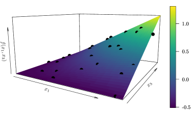
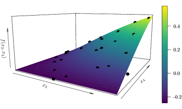
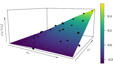
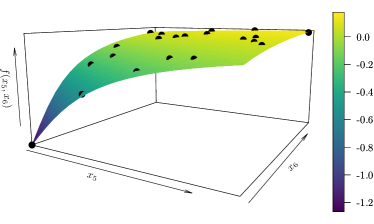
Figure 8: 2D visualizations of (left) the centered functions $y_{1}:(x_{1},x_{3})\mapsto 2x_{1}x_{3}$ (top), $y_{2}:(x_{2},x_{4})\mapsto\sin(x_{2}x_{4})$ (middle) and $y_{3}:(x_{5},x_{6})\mapsto\tan(3x_{5}+5x_{6})$ (bottom), and their corresponding constructed predictors (right).

E.2 Analysis for the coastal flooding case

As developed in Section 5.3 and seen from Figures 5, 6 and 7, the additive structure of the function is $f(S,T,\phi,t_{+},t_{-})=f_{1}(S,T,\phi)+f_{2}(t_{+})+f_{3}(t_{-})$. We will study the block-predictor of the function $f_{1}$ by showing bivariate representations of the functions $f_{1}(\cdot,\cdot,\phi)$ for various values of $\phi$.

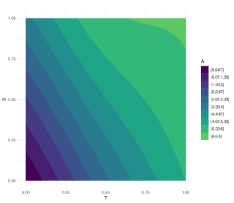
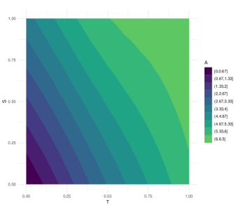
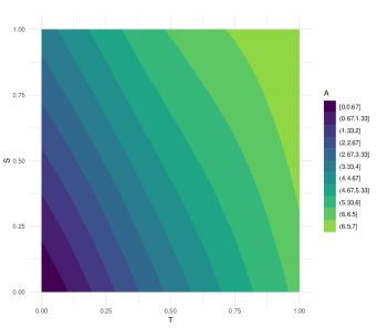
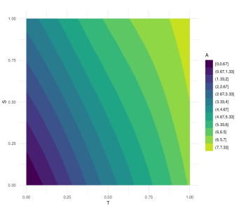
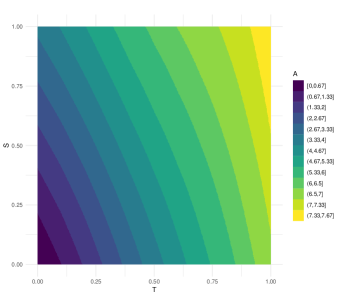
Figure 9: Bivariate representation of the functional relationship between $S$ and $T$ given $(\cos(\phi)+1)/2=0,1/4$ (top), $(\cos(\phi)+1)/2=1/2,3/4$ (middle), $(\cos(\phi)+1)/2=1$ (bottom).

Figure 9 highlights that for fixed $\phi$, the function $(T,S)\mapsto f_{1}(T,S,\phi)$ is quasi-linear. Only for high values of $T$ and $S$ we observe non-linear interactions. Indeed, the isolines for small values of $S$ and $T$ are lines equally spaced, meaning that the function $f_{1}(\cdot,\cdot,\phi)$ behaves as a linear function. Moreover, the vertical orientations of the isolines indicate that the variable $T$ has more impact over the coastal flooding than $S$ which coincides with the Sobol analysis obtained in Figure 5.

One can notice that the influence of the tide $T$ over the coastal flooding increases as the phase difference $\phi$ decreases. We can deduce that the coastal flooding is more sensitive to the tide when the latter is synchronised with the surge. On the other hand, it seems that the influence of the surge over the coastal flooding does not increase as $\phi$ decreases.

These observations are natural as the range of the tide $T$ is wider than the range of the surge $S$ before renormalization as in Figure 5.

References

- [1] C. E. Rasmussen and C. K. I. Williams, Gaussian Processes for Machine Learning. Cambridge, MA: The MIT Press, 2005.
- [2] J. Sacks, W. Welch, T. Mitchell, and H. Wynn, “Design and analysis of computer experiments,” Statistical Science, vol. 4, pp. 409–423, 1989.
- [3] D. R. Jones, M. Schonlau, and W. J. Welch, “Efficient global optimization of expensive black-box functions,” Journal of Global Optimization, vol. 13, no. 4, pp. 455–492, Dec 1998.
- [4] F. Bachoc, C. Helbert, and V. Picheny, “Gaussian process optimization with failures: Classification and convergence proof,” Journal of Global Optimization, vol. 78, no. 3, pp. 483–506, 2020.
- [5] M. C. Kennedy and A. O’Hagan, “Bayesian calibration of computer models,” Journal of the Royal Statistical Society: Series B (Statistical Methodology), vol. 63, no. 3, pp. 425–464, 2001.
- [6] J.-P. Chiles and P. Delfiner, Geostatistics: Modeling Spatial Uncertainty. John Wiley & Sons, 2009.
- [7] M. Niu, P. Cheung, L. Lin, Z. Dai, N. Lawrence, and D. Dunson, “Intrinsic Gaussian processes on complex constrained domains,” Journal of the Royal Statistical Society: Series B (Statistical Methodology), vol. 81, no. 3, pp. 603–627, 2019.
- [8] S. Da Veiga and A. Marrel, “Gaussian process modeling with inequality constraints,” Annales de la faculté des sciences de Toulouse Mathématiques, vol. 21, no. 3, pp. 529–555, 2012.
- [9] S. Da Veiga and A. Marrel, “Gaussian process regression with linear inequality constraints,” Reliability Engineering & System Safety, vol. 195, p. 106732, 2020.
- [10] P. Ray, D. Pati, and A. Bhattacharya, “Efficient bayesian shape-restricted function estimation with constrained gaussian process priors,” Statistics and Computing, vol. 30, pp. 839–853, 2020.
- [11] J. Wang, J. Cockayne, and C. J. Oates, “A role for symmetry in the Bayesian solution of differential equations,” Bayesian Analysis, vol. 15, no. 4, pp. 1057 – 1085, 2020.
- [12] F. Bachoc, A. Lagnoux, and A. F. López-Lopera, “Maximum likelihood estimation for Gaussian processes under inequality constraints,” Electronic Journal of Statistics, vol. 13, no. 2, pp. 2921–2969, 2019.
- [13] J. Riihimäki and A. Vehtari, “Gaussian processes with monotonicity information,” in International Conference on Artificial Intelligence and Statistics, 2010, pp. 645–652.
- [14] S. Golchi, D. R. Bingham, H. Chipman, and D. A. Campbell, “Monotone emulation of computer experiments,” SIAM/ASA Journal on Uncertainty Quantification, vol. 3, no. 1, pp. 370–392, 2015.
- [15] A. Cousin, H. Maatouk, and D. Rullière, “Kriging of financial term-structures,” European Journal of Operational Research, vol. 255, no. 2, pp. 631–648, 2016.
- [16] H. Maatouk and X. Bay, “Gaussian process emulators for computer experiments with inequality constraints,” Mathematical Geosciences, vol. 49, no. 5, pp. 557–582, 2017.
- [17] A. F. López-Lopera, F. Bachoc, N. Durrande, and O. Roustant, “Finite-dimensional Gaussian approximation with linear inequality constraints,” SIAM/ASA Journal on Uncertainty Quantification, vol. 6, no. 3, pp. 1224–1255, 2018.
- [18] A. F. López-Lopera, S. John, and N. Durrande, “Gaussian process modulated Cox processes under linear inequality constraints,” in International Conference on Artificial Intelligence and Statistics, 2019, pp. 1997–2006.
- [19] A. F. López-Lopera, F. Bachoc, N. Durrande, J. Rohmer, D. Idier, and O. Roustant, “Approximating Gaussian process emulators with linear inequality constraints and noisy observations via MC and MCMC,” in Monte Carlo and Quasi-Monte Carlo Methods. Cham: Springer International Publishing, 2020, pp. 363–381.
- [20] S. Zhou, P. Giulani, J. Piekarewicz, A. Bhattacharya, and D. Pati, “Reexamining the proton-radius problem using constrained Gaussian processes,” Physical Review C, vol. 99, p. 055202, 2019.
- [21] F. Bachoc, A. F. López-Lopera, and O. Roustant, “Sequential construction and dimension reduction of gaussian processes under inequality constraints,” SIAM Journal on Mathematics of Data Science, vol. 4, no. 2, pp. 772–800, 2022.
- [22] T. J. Hastie, “Generalized additive models,” in Statistical models in S. Routledge, 2017, pp. 249–307.
- [23] A. Buja, T. Hastie, and R. Tibshirani, “Linear smoothers and additive models,” The Annals of Statistics, pp. 453–510, 1989.
- [24] N. Durrande, D. Ginsbourger, and O. Roustant, “Additive covariance kernels for high-dimensional Gaussian process modeling,” Annales de la Faculté de Sciences de Toulouse, vol. 21, no. 3, pp. 481–499, 2012.
- [25] D. K. Duvenaud, H. Nickisch, and C. E. Rasmussen, “Additive Gaussian processes,” in Neural Information Processing Systems, 2011, pp. 226–234.
- [26] A. López-Lopera, F. Bachoc, and O. Roustant, “High-dimensional additive Gaussian processes under monotonicity constraints,” Neural Information Processing Systems, vol. 35, pp. 8041–8053, 2022.
- [27] C. B. Storlie, H. D. Bondell, B. J. Reich, and H. H. Zhang, “Surface estimation, variable selection, and the nonparametric oracle property,” Statistica Sinica, vol. 21, no. 2, p. 679, 2011.
- [28] C. J. Stone, “Additive regression and other nonparametric models,” The annals of Statistics, vol. 13, no. 2, pp. 689–705, 1985.
- [29] S. N. Wood, Z. Li, G. Shaddick, and N. H. Augustin, “Generalized additive models for gigadata: Modeling the UK black smoke network daily data,” Journal of the American Statistical Association, vol. 112, no. 519, pp. 1199–1210, 2017.
- [30] D. Azzimonti, D. Ginsbourger, J. Rohmer, and D. Idier, “Profile extrema for visualizing and quantifying uncertainties on excursion regions: Application to coastal flooding,” Technometrics, 2019.
- [31] X. Bay, L. Grammont, and H. Maatouk, “Generalization of the kimeldorf-wahba correspondence for constrained interpolation,” Electronic Journal of Statistics, vol. 10, no. 1, pp. 1580–1595, May 2016.
- [32] H. Maatouk and X. Bay, “A new rejection sampling method for truncated multivariate Gaussian random variables restricted to convex sets,” in Monte Carlo and Quasi-Monte Carlo Methods. Cham: Springer International Publishing, 2016, pp. 521–530.
- [33] H. Maatouk, D. Rullière, and X. Bay, “Efficient constrained Gaussian process approximation using elliptical slice sampling,” 2024, HAL preprint (hal-04496474).
- [34] A. F. López-Lopera and M. Deronzier, lineqGPR: Gaussian process regression with linear inequality constraints, 2022, R] package version 0.3.0. [Online]. Available: https://github.com/anfelopera/lineqGPR
- [35] M. Stein, “Large sample properties of simulations using Latin hypercube sampling,” Technometrics, vol. 29, no. 2, pp. 143–151, 1987.
- [36] A. Pakman and L. Paninski, “Exact Hamiltonian Monte Carlo for truncated multivariate Gaussians,” Journal of Computational and Graphical Statistics, vol. 23, no. 2, pp. 518–542, 2014.
- [37] G. Wahba, Spline models for observational data. SIAM, 1990.
- [38] D. Azzimonti, “profExtrema: Compute and visualize profile extrema functions,” R package version 0.2.0, 2018.
- [39] J. Rohmer, D. Idier, F. Paris, R. Pedreros, and J. Louisor, “Casting light on forcing and breaching scenarios that lead to marine inundation: Combining numerical simulations with a random-forest classification approach,” Environmental modelling & software, vol. 104, pp. 64–80, 2018.
- [40] O. Roustant, D. Ginsbourger, and Y. Deville, “DiceKriging, DiceOptim: Two R packages for the analysis of computer experiments by Kriging-based metamodeling and optimization,” Journal of Statistical Software, vol. 51, no. 1, pp. 1–55, 2012. [Online]. Available: https://www.jstatsoft.org/v51/i01/
- [41] T. Muehlenstaedt, O. Roustant, L. Carraro, and S. Kuhnt, “Data-driven Kriging models based on FANOVA-decomposition,” Statistics and Computing, vol. 22, pp. 723–738, 2012.
- [42] J. Fruth, O. Roustant, and S. Kuhnt, “Total interaction index: A variance-based sensitivity index for second-order interaction screening,” Journal of Statistical Planning and Inference, vol. 147, pp. 212–223, 2014.
- [43] R. Liu and A. B. Owen, “Estimating mean dimensionality of analysis of variance decompositions,” Journal of the American Statistical Association, vol. 101, no. 474, pp. 712–721, 2006.
- [44] F. Bachoc, A. Lagnoux, and A. F. López-Lopera, “Maximum likelihood estimation for Gaussian processes under inequality constraints,” Electronic Journal of Statistics, vol. 13, no. 2, pp. 2921–2969, 2019.