SceneMotion: From Agent-Centric Embeddings to Scene-Wide Forecasts

Abstract

Self-driving vehicles rely on multimodal motion forecasts to effectively interact with their environment and plan safe maneuvers. We introduce SceneMotion, an attention-based model for forecasting scene-wide motion modes of multiple traffic agents. Our model transforms local agent-centric embeddings into scene-wide forecasts using a novel latent context module. This module learns a scene-wide latent space from multiple agent-centric embeddings, enabling joint forecasting and interaction modeling. The competitive performance in the Waymo Open Interaction Prediction Challenge demonstrates the effectiveness of our approach. Moreover, we cluster future waypoints in time and space to quantify the interaction between agents. We merge all modes and analyze each mode independently to determine which clusters are resolved through interaction or result in conflict. Our implementation is available at: https://github.com/kit-mrt/future-motion

Figure 1: SceneMotion. Our attention-based motion forecasting model is composed of stacked encoder and decoder modules. Variable-sized agent-centric views $V_{i}$ are reduced to fixed-sized agent-centric embeddings $E_{i}$ via cross-attention with road environment descriptor (RED) tokens $R_{j}$. Afterwards, we concatenate the agent-centric embeddings with global reference tokens $G_{i}$ and rearrange them to form a scene-wide embedding. Our latent context module then learns global context and our motion decoder transforms learned anchors $A_{k}$ into scene-wide forecasts. We show a simplified example with only two focal agents. By default, our model forecasts motion for 8 focal agents each with 48 context agents, enabling interaction modeling in complex scenarios.

I Introduction

Future motion in traffic scenarios is inherently multimodal. Multiple types of agents such as vehicles, pedestrians, or cyclists can move and interact in multiple ways. Therefore, self-driving vehicles rely on multimodal motion forecasts to successfully interact with their environment and plan safe maneuvers [1, 2]. Motion forecasting methods predict future motion based on past observations and scene context (e.g., lane data and traffic light states). However, the majority of recent methods (e.g., [3, 4]) forecast motion for each agent individually (i.e., marginal prediction), which omits modeling of future interaction between agents.

In this work, we present SceneMotion, an attention-based model for forecasting scene-wide motion modes of multiple traffic agents. Our model transforms local agent-centric embeddings into scene-wide forecasts using a novel latent context module. We use agent-centric representations since they allow for more data-efficient learning than scene-centric representations (as in e.g., [5]). In particular, they generate more training samples (potentially for each agent in a traffic scene) and share the local reference frame with motion forecasts. In contrast to fully agent-centric models (e.g., [3, 6]), we use local agent-centric views that capture information from a smaller area of the map. Afterwards, our latent context module learns a scene-wide latent space from multiple agent-centric embeddings, enabling joint forecasting and interaction modeling.

Recent methods address interpretability in motion forecasting by engineering learned representations [7, 8] or learning intention goals [9, 10]. We interpret scene-wide motion forecasts in terms of clusters of waypoints to quantify the interaction between agents. Waypoint clusters are related to implicit occupancy forecasts [11, 12], but explicitly represent which agents are likely to interact. This expands the contextual information available to motion planners.

Overall, our main contributions are twofold:

1. We present SceneMotion, an attention-based and data-efficient model for forecasting scene-wide motion modes.

2. We propose to analyze scene-wide motion forecasts in terms of clusters of waypoints to quantify future interaction.

II Related work

Joint motion forecasting methods model the joint distribution of future motions of multiple agents. Related methods use attention mechanisms between latent representations to model interactions and decode joint futures [13, 5, 14, 15]. Seff et al. [16] cast motion forecasting as language modeling and autoregressively decode joint sets of discrete motion vectors. Their autoregressive decoding allows for temporal causal conditioning, but leads to high inference latency. Jiang et al. [17] reformulate joint motion forecasting as conditional denoising diffusion process. They condition a learned denoiser on environment context to transform a set of noisy trajectories (i.e., positions disturbed by Gaussian noise) into a joint set of future trajectories. At inference, trajectories are sampled from pure noise, causing high inference latency.

Conditional motion forecasting methods forecast future motion for one agent conditioned on the forecast for one [18, 19] or multiple other agents [20, 21, 22]. For scene-wide forecasts, iterative rollouts are used to successively condition forecasts on each other, resulting in high inference latency for complex traffic scenarios. However, goal conditioned motion forecasting [5, 23] bridges the gap to planning and relaxes the conditioning from a full future trajectory to a goal point (i.e., destination).

Marginal motion forecasting methods model future motion for each agent individually. Related methods extend marginal forecasting models with auxiliary joint [24, 25] or dense prediction [10] objectives to model future interactions in a second step. However, this limits interaction modeling to recombining otherwise independent forecasts.

Data-efficient learning is about learning good representations from limited data. For motion forecasting, a recent approach to data efficient learning is self-supervised learning [26, 27, 28]. These methods perform self-supervised pre-training followed by supervised fine-tuning using less annotated or the same data to improve downstream performance (i.e., motion forecasting accuracy).

III Method

Our proposed model, SceneMotion, is attention-based and forecasts scene-wide motion modes in self-driving applications (see Fig. 1). We define scene-wide motion forecasting as modeling joint distributions of future trajectories for multiple agents from past trajectories and scene context (e.g., lanes and traffic light states). Hence, a scene-wide motion mode describes a joint set of future trajectories with one trajectory for each modeled agent. A trajectory represents a sequence of waypoints and a waypoint is a 2D position with $x$ and $y$ coordinates. Therefore, scene-wide motion forecasting requires scene-wide representations to model future motion for multiple agents, including interaction.

Related work focuses on improving the computational efficiency by using scene-centric [5, 14] or pairwise relative representations [29, 30]. Such representations reduce the amount of repeated computations compared to agent-centric input representations. We argue that both approaches are less data-efficient than agent-centric input representations. Scene-centric methods encode all agent and map data in a common reference frame, generating only one sample per scene versus one sample for each agent. Furthermore, motion forecasts are typically in an agent-centric reference frame starting at $(x,y)=(0,0)$, which requires scene-centric models to learn the transformation from a scene-centric to an agent-centric reference frame. Pairwise relative methods encode map data once per scene and agent history for each agent. As a result, agent representations are learned in a data-efficient manner, while map representations are not.

While agent-centric representations offer improved data efficiency, they can lead to redundant computations due to overlapping data. Our model addresses this using local input views, which cover a smaller map area than in fully agent-centric models (e.g., [3, 6, 4]). Afterwards, our latent context module learns a scene-wide latent space from multiple agent-centric embeddings, enabling joint forecasting and interaction modeling. In the following, we discuss specific representations and modules in our model in more detail.

Input representation: We follow [31, 30] and represent all processed modalities (i.e., past motion, map data, and traffic light states) as polylines. For past motion, these polylines contain spatiotemporal data: past positions, past orientations, past velocities, dimensions, and temporal order as one-hot encodings. We sample temporal features with a frequency of 10 Hz. For lane data and traffic lights, the polyline representations include node positions and classes (e.g., lane types and current traffic light states). We generate local agent-centric input views ($V_{i}$ in Fig. 1, where $i$ is the agent index) including the 128 nearest map polylines and 48 other context agents. For reference, the fully agent-centric Wayformer model [3] and the pairwise relative HPTR model [30] process the nearest 512 map polylines.

Agent-centric modules: Our local encoder is a multilayer perceptron (MLP) with 3 layers, which projects all agent-centric polylines to vectors of dimension 256. Afterwards, we add learned absolute positional embeddings [32]. The resulting vector sets per agent-centric view have different lengths depending on the complexity of the corresponding local map area. Therefore, we use a learned reduction mechanism [33] to transform these agent-centric views into fixed-size agent-centric embeddings (see $E_{i}$ in Fig. 1). Our reduction decoder includes 4 blocks of alternating self-attention, cross-attention, LayerNorm, and FeedForward layers. The self-attention blocks mix features within $V_{i}$, and the cross-attention blocks extract features from $V_{i}$ into learned road environment descriptor (RED) tokens $R_{j}$. Consequently, each $E_{i}$ embedding has the same fixed size of 128 tokens as the set of learned RED tokens.

Scene-wide modules: To form a scene-wide embedding, we concatenate the agent-centric embeddings with global reference tokens $G_{i}$ and rearrange them. $G_{i}$ tokens are learned as linear projections of rotation and translation vectors for agent-centric views into a common scene-wide reference frame. Our rearranging changes the batch dimension from the agent index to the scene index. Therefore, our model has a dynamic batch size that changes between our agent-centric and scene-wide modules. Afterwards, our latent context module learns global context via 6 blocks of self-attention, LayerNorm, and FeedForward layers. Finally, we use an attention-based motion decoder with an MLP-based head to transform learned anchors $A_{k}$ into $k=6$ motion modes.

Split	Method (config)	Venue	mAP $\uparrow$	minSADE $\downarrow$	minSFDE $\downarrow$	MR $\downarrow$	OR $\downarrow$
Test	Scene Transformer (joint) [5]	ICLR’22	0.1192	0.9774	2.1892	0.4942	0.2067
	M2I [25]	CVPR’22	0.1239	1.3506	2.8325	0.5538	0.2757
	GameFormer (joint) [34]	ICCV’23	0.1376	0.9161	1.9373	0.4531	0.2112
	SceneMotion (ours)		0.1789	1.0044	2.3141	0.5331	0.2163
	MotionLM (ensemble)	ICCV’23	0.2178	0.8911	2.0067	0.4115	-
Val	GameFormer (joint) [34]	ICCV’23	0.1339	0.9133	1.9251	0.4564	-
	MotionLM (single replica) [16]	ICCV’23	0.1687	1.0345	2.3886	0.4943	-
	JFP (Wayformer) [24]	CoRL’23	0.1700	0.9500	2.1700	0.4500	-
	SceneMotion (ours)		0.1793	0.9613	2.2085	0.5137	0.2129
	Wayformer (marginal) [3, 24]	ICRA’23	0.1600	0.9900	2.3000	0.4700	-

TABLE I: Comparison of joint motion forecasting methods. All methods are evaluated on the interactive splits of the Waymo Open Motion Dataset [35]. Following [30], we compare our method with real-time capable single replica versions of recent motion forecasting methods. We show the results of a non-realtime capable ensemble and a state-of-the-art marginal forecasting model for reference. Best scores are bold, second best are underlined.

Output representation: We follow common practice (e.g., [3, 30]) and represent future motion as mixture of Gaussians, with the following mean and covariance parameters for 2D positions: $\mu_{x},\mu_{y},\sigma_{x},\sigma_{y},\rho$. We forecast motion with a sampling frequency of 10 Hz. During training, we minimize the negative log-likelihood (NLL) loss for predicted positions and the cross-entropy loss for the corresponding confidence scores. To learn joint modes of scene-wide forecasts, we use a winner-takes-all assignment to select the best of 6 scene-wide trajectory sets. Specifically, we only backpropagate the loss for the set with the lowest average displacement error [36, 5].

IV Benchmarking motion forecasts

In this section, we compare our method to recent motion forecasting methods using the large-scale Waymo Open Motion Dataset [35]. We focus our comparison on joint motion forecasting, but discuss marginal performance as well.

Dataset: The Waymo Open Motion Dataset includes over 1.1 million data points extracted from 103,000 urban or suburban driving scenarios, spanning 20 seconds each. The state of traffic agents includes attributes like class (i.e., vehicle, pedestrian, or cyclist), position, dimensions, velocity, acceleration, orientation, angular velocity, and the status of turn signals. Each data point captures 1 second of past followed by 8 seconds of future data. We resample this time interval with 10 Hz. The map data is represented as polylines and includes multiple lane types, crosswalks, speed bumps, stop signs, and traffic lights with their states.

Training details: We configure our model as described in section III, which corresponds to a transformer model with 19 M trainable parameters. We sample 28 scenes in a batch, with 8 focal (i.e., predicted) agents per scene. Consequently, our agent-centric modules are trained with a batch size of 224 and our scene-wide modules with a batch size of 28. We use Adam with weight decay [37] as the optimizer and a step learning rate scheduler to halve the initial learning rate of $2^{-4}$ every 20 epochs. We train for 50 epochs using data distributed parallel (DDP) training on 4 A6000 GPUs.

Evaluation metrics: We use the official challenge metrics, the mean average precision (mAP), the average displacement error (minADE), and the final displacement error (minFDE), the miss rate (MR), and the overlap rate (OR) to evaluate motion forecasts. All metrics are computed using the minimum mode for $k=6$ modes. Accordingly, the metrics for the mode closest to the ground truth are measured. Joint modes (i.e., best scene-wide mode) are evaluated on the interactive splits (denoted by an additional S in the metric names) and marginal modes (i.e., best mode for each agent individually) on the regular splits. All metrics are averaged over the three prediction horizons of 3 s, 5 s, and 8 s, and the 3 agent classes (vehicles, pedestrians, and cyclists). Refer to the appendix for the complete results of our model.

Joint motion forecasting performance: Table I shows the results of our method on the official Waymo Interaction Prediction challenge. Therefore, all metrics are scene-wide and computed for joint modes. Following [30], we compare against real-time capable single replica versions of joint motion forecasting methods and marginal methods with auxiliary joint motion forecasting objectives. Additionally, we show the results of a non-realtime capable ensemble of 8 MotionLM models and a state-of-the-art marginal motion forecasting model (Wayformer) for reference. In both splits (test and validation), our method outperforms all comparable methods on the main challenge metric, the mAP. In particular, our model outperforms a single replica of MotionLM; only a non-real-time capable ensemble of 8 replicas achieves higher mAP values on the test set. For most of the remaining metrics, our model ranks third.

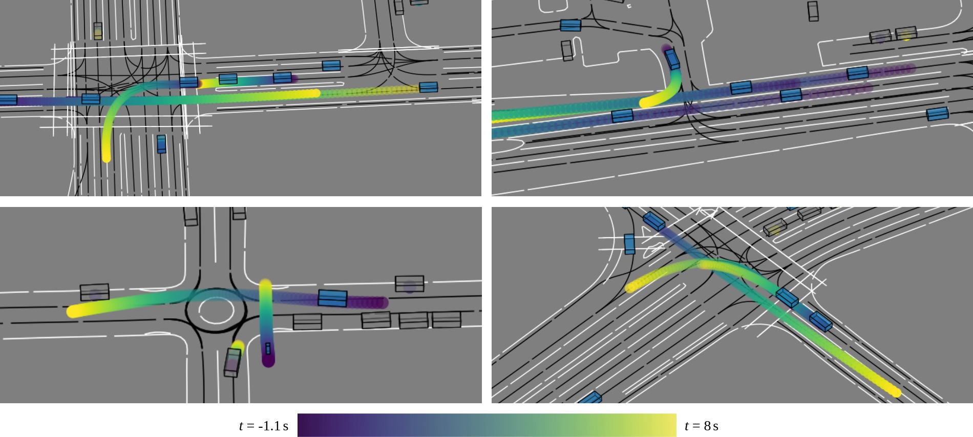
Figure 2: Scene-wide motion forecasts. Our model forecasts scene-wide motion modes by modeling joint distributions of trajectories for 8 focal agents. Dynamic agents are shown in blue, static agents in grey (determined at $t=0\,\text{s}$). Lanes are black lines and road markings are white lines.

Furthermore, all joint models except GameFormer outperform the marginal Wayformer model, underscoring the importance of joint motion forecasting for interaction modeling. Fig. 2 shows qualitative results from the interactive split of the Waymo Open Motion dataset.

Marginal motion forecasting performance: Our model is flexible with respect to forecasting types and can be configured to forecast marginal distributions of trajectories (i.e., for each agent independently). Specifically, we fine-tune our previously trained model for marginal forecasting by changing the winner-takes-all assignment to choose the best mode per agent instead of the best scene-wide mode. We fine-tune for another 40 epochs, for a total of 90 epochs, and keep the training hyperparameters the same as in the initial training. Table II shows that our model achieves competitive results on marginal motion forecasting metrics as well.

Method (config)	Venue	mAP $\uparrow$	minADE $\downarrow$	minFDE $\downarrow$	#Epochs	$T_{\text{epoch}}$	$T_{\text{train}}$
Scene Transformer (marginal) [5]	ICLR’22	-	0.6130	1.2200	-	-	-
MTR [6]	NeurIPS’22	0.4164	0.6046	1.2251	-	-	-
HPTR [30]	NeurIPS’23	0.4150	0.5378	1.0923	120	52 min	104 h
SceneMotion (ours, marginal)		0.4251	0.5464	1.1202	90	22 min	33 h

TABLE II: Marginal motion forecasting performance and training time. All methods are evaluated on the regular validation split of the Waymo Open Motion Dataset [35]. $T_{\text{epoch}}$ and $T_{\text{train}}$ are measured for training runs with 4 A6000 GPUs. Best scores are bold, second best are underlined.

Training time: We compare the required training epochs with those of the recent pairwise relative model HPTR. Our two-stage training (first joint, then marginal) is 90 epochs long, compared to the 120 epochs recommended for HPTR. Since our model allows for larger batch sizes on the same hardware, the time required to train one epoch is more than 50% shorter. As a result, the total training time $T_{\text{train}}$ of our model is only about one third of the time required to train HPTR using A6000 GPUs (see Table II).

V Analyzing clusters of future waypoints

In this section, we propose a method to quantify future interaction based on our multimodal motion forecasts. Our method clusters future waypoints to determine which agents are likely to interact in the future. We compute clusters for all agents over all modes in each timestep (i.e., we initially discard motion modes by merging trajectories from all modes). Afterwards, we evaluate if our forecasting model resolves the waypoint clusters by modeling the interaction between agents. In particular, we verify that the clusters do not exist within joint modes. Vice versa, if the cluster exists within a joint motion mode, a future conflict is more likely. Thus, in subsequent planning, trajectories with waypoint clusters can be associated with higher risk [38, 39, 40].

Specifically, we use the DBSCAN algorithm [41] for clustering, with a max. distance of 2.5 m and a min. number of 2 waypoints per cluster. Unlike clustering algorithms that require specifying the number of clusters beforehand (e.g., $k$-means), DBSCAN clusters waypoints more reliably by choosing a suitable number of clusters depending on the given data.

For illustration, we show an example of two interacting agents in Fig. 3, yet our method scales to an arbitrary number of agents. In Fig. 3 (a), waypoints of the lower vehicle that form clusters with waypoints of another vehicle are highlighted in orange. The vehicle potentially involved in the interaction is connected to these waypoints by dashed orange lines. Fig. 3 (b) shows all trajectories for the corresponding vehicles leading to the waypoint clusters. Since our model is trained to forecast consistent modes with respect to the future motion of agents, waypoint clusters are less likely within joint modes. For example, Fig. 3 (c) shows the trajectories of the involved vehicles from the top-1 (i.e., most likely) joint motion mode, which does not include a waypoint cluster. Thus, our forecasting model likely resolves the cluster by modeling the interaction between the two vehicles.

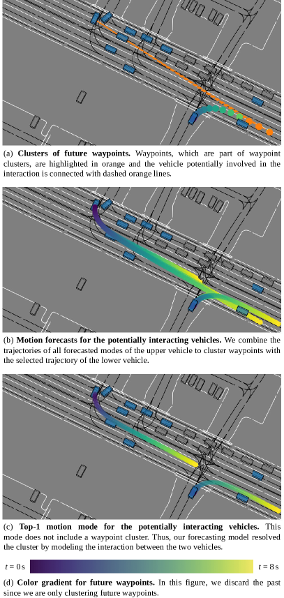
Figure 3: Analyzing scene-wide motion forecasts in terms of waypoint clusters. We show an example of a potential interaction of widely separated vehicles to demonstrate the benefits of a long prediction horizon of 8 s.

We evaluate our method on the interactive validation split of the Waymo Open Motion Dataset. The results are shown in Table III. When clustering the merged set of waypoints from all motion modes, $29.42\%$ of the agents have clustered waypoints with other agents. This shows a large number of possible future interactions.

Notably, the percentage of agents with clustered waypoints decreases to $13.52\%$ when all modes are considered independently and to $6.55\%$ when only the top-1 mode is considered.

Furthermore, we evaluate the learned assignment of trajectories to scene-wide modes by comparing it to a random assignment scheme. Specifically, we compute the average percentage of agents with clustered waypoints within the forecasted modes versus with random mode assignment per trajectory. We implement the random assignment scheme by sampling mode indices for each trajectory from a discrete uniform distribution on the integer interval $[0\,..\,5]$. Within the resulting modes of randomly shuffled trajectories, we compute the percentage of agents with clustered waypoints. We repeat this process 6 times per scene and take the average (see “Avg random mode per trajectory” in Table III). The average percentage of agents with clustered waypoints is 23% lower within the forecasted modes (i.e., using the learned assignment) than with random assignment (6.65% versus 8.69%).

Overall, the results indicate that our motion forecasting model is capable of interaction modeling and resolving potential future conflicts.

Evaluation type	Clustered agents $\downarrow$
All modes merged	$29.42$%
Top-1 mode	$6.55$%
Top-3 modes	$10.12$%
Top-6 modes	$13.52$%
Avg random mode per trajectory	8.69%
Avg within modes	6.65%

TABLE III: Percentage of agents with clustered waypoints. “All modes merged” refers to clustering waypoints from all modes, while “Top-$k$ modes” refers to clustering within $k$ modes independently. “Avg random mode per trajectory” refers to the average of 6 iterations of random sampling of mode indices per trajectory. “Avg within modes” refers to the average of the 6 forecasted modes using the learned mode indices.

VI Conclusion and future work

In this work, we have introduced a method for transforming local agent-centric embeddings into scene-wide motion forecasts. Inspired by methods that perform self-supervised pre-training, we use local agent-centric views for more data-efficient learning compared to existing scene-centric and pairwise relative representations. Our novel latent context module subsequently learns a scene-wide latent space from multiple agent-centric embeddings, enabling joint motion forecasting and interaction modeling. Evaluations on the Waymo Open Motion Dataset and the Waymo Open Interaction Prediction Challenge confirm the effectiveness of our method.

Furthermore, we have proposed to cluster future waypoints in time and space to quantify the interaction between agents.We merge all modes and analyze each mode independently to determine whether a cluster is likely resolved by interaction or results in conflict.

Future work includes exploring how motion planners can benefit from additional information about interactions and the use of mixture models for specific agents and scenarios.

(95mm,20mm) Appendix

Object Type	Measurement time (s)	soft mAP $\uparrow$	mAP $\uparrow$	minADE $\downarrow$	minFDE $\downarrow$	MR $\downarrow$	OR $\downarrow$
Vehicle	3	0.3649	0.3466	0.4016	0.8177	0.2962	0.0421
Vehicle	5	0.2405	0.2295	0.8685	1.9423	0.4363	0.1245
Vehicle	8	0.1371	0.1319	1.8969	4.6197	0.6019	0.3184
Vehicle	Avg	0.2475	0.2360	1.0557	2.4599	0.4448	0.1616
Pedestrian	3	0.3218	0.3104	0.3128	0.6283	0.3646	0.2195
Pedestrian	5	0.2118	0.2040	0.6669	1.4729	0.5170	0.2959
Pedestrian	8	0.1352	0.1346	1.4081	3.3252	0.6932	0.4419
Pedestrian	Avg	0.2229	0.2164	0.7959	1.8088	0.5250	0.3191
Cyclist	3	0.1567	0.1512	0.4755	0.9547	0.5015	0.0673
Cyclist	5	0.0759	0.0736	0.9836	2.1837	0.6148	0.1498
Cyclist	8	0.0284	0.0280	2.0260	4.8828	0.7725	0.2876
Cyclist	Avg	0.0870	0.0843	1.1617	2.6737	0.6296	0.1682
All	3	0.2812	0.2694	0.3967	0.8002	0.3874	0.1096
All	5	0.1761	0.1691	0.8397	1.8663	0.5227	0.1901
All	8	0.1002	0.0982	1.7770	4.2759	0.6892	0.3493
All	Avg	0.1858	0.1789	1.0044	2.3141	0.5331	0.2163

TABLE IV: Test metrics by object type and measurement time for joint motion forecasting.

Object Type	Measurement time (s)	soft mAP $\uparrow$	mAP $\uparrow$	minADE $\downarrow$	minFDE $\downarrow$	MR $\downarrow$	OR $\downarrow$
Vehicle	3	0.3835	0.3678	0.3953	0.8006	0.2864	0.0396
Vehicle	5	0.2622	0.2543	0.8491	1.8859	0.4225	0.1205
Vehicle	8	0.1788	0.1757	1.8448	4.4780	0.5906	0.3132
Vehicle	Avg	0.2748	0.2659	1.0297	2.3882	0.4332	0.1578
Pedestrian	3	0.3070	0.2944	0.2990	0.5890	0.3542	0.2185
Pedestrian	5	0.1946	0.1896	0.6175	1.3270	0.4681	0.2928
Pedestrian	8	0.0725	0.0691	1.2874	2.9752	0.6350	0.4306
Pedestrian	Avg	0.1914	0.1844	0.7346	1.6304	0.4858	0.3139
Cyclist	3	0.1624	0.1579	0.4582	0.9194	0.4974	0.0688
Cyclist	5	0.0774	0.0760	0.9431	2.0950	0.6151	0.1436
Cyclist	8	0.0288	0.0285	1.9576	4.8060	0.7536	0.2884
Cyclist	Avg	0.0895	0.0875	1.1196	2.6068	0.6221	0.1669
All	3	0.2843	0.2734	0.3842	0.7697	0.3793	0.1090
All	5	0.1781	0.1733	0.8032	1.7693	0.5019	0.1856
All	8	0.0933	0.0911	1.6966	4.0864	0.6598	0.3441
All	Avg	0.1852	0.1793	0.9613	2.2085	0.5137	0.2129

TABLE V: Validation metrics by object type and measurement time for joint motion forecasting.

Object Type	Measurement time (s)	soft mAP $\uparrow$	mAP $\uparrow$	minADE $\downarrow$	minFDE $\downarrow$	MR $\downarrow$	OR $\downarrow$
Vehicle	3	0.5674	0.5493	0.2825	0.4930	0.0902	0.0187
Vehicle	5	0.4574	0.4502	0.5757	1.1109	0.1313	0.0384
Vehicle	8	0.3374	0.3342	1.1128	2.4611	0.2091	0.0940
Vehicle	Avg	0.4541	0.4446	0.6570	1.3550	0.1435	0.0503
Pedestrian	3	0.5580	0.5380	0.1495	0.2716	0.0511	0.2384
Pedestrian	5	0.4658	0.4571	0.2818	0.5510	0.0676	0.2643
Pedestrian	8	0.4175	0.4105	0.4884	1.0322	0.0881	0.2593
Pedestrian	Avg	0.4804	0.4687	0.3066	0.6182	0.0689	0.2660
Cyclist	3	0.4438	0.4342	0.3350	0.6021	0.1855	0.0472
Cyclist	5	0.3665	0.3629	0.6156	1.1827	0.1946	0.0846
Cyclist	8	0.2734	0.2715	1.0773	2.3639	0.2432	0.1378
Cyclist	Avg	0.3612	0.3562	0.6760	1.3829	0.2078	0.0898
All	3	0.5231	0.5073	0.2557	0.4556	0.1089	0.1014
All	5	0.4299	0.4234	0.4910	0.9482	0.1312	0.1291
All	8	0.3428	0.3387	0.8928	1.9524	0.1801	0.1757
All	Avg	0.4319	0.4232	0.5465	1.1187	0.1401	0.1354

TABLE VI: Validation metrics by object type and measurement time for marginal motion forecasting.

Focal agents	Inference latency
2	54.3 ms
8 (default)	59.7 ms
64	191.1 ms

TABLE VII: Inference latency of our SceneMotion model. We measure the inference latency on one A6000 GPU using the PyTorch Lightning profiler and plain eager execution. We report the average of 1000 iterations per configuration for the complete predict_step, including pre- and post-processing.

References

- [1] Ömer Şahin Taş, Philipp Heinrich Brusius and Christoph Stiller “Decision-theoretic MPC: Motion Planning with Weighted Maneuver Preferences Under Uncertainty” In arXiv: 2310.17963, 2023
- [2] Haruki Nishimura, Jean Mercat, Blake Wulfe, Rowan Thomas McAllister and Adrien Gaidon “RAP: Risk-Aware Prediction for Robust Planning” In Conference on Robot Learning (CoRL), 2023
- [3] Nigamaa Nayakanti, Rami Al-Rfou, Aurick Zhou, Kratarth Goel, Khaled S Refaat and Benjamin Sapp “Wayformer: Motion Forecasting via Simple & Efficient Attention Networks” In IEEE International Conference on Robotics and Automation (ICRA), 2023
- [4] Xishun Wang, Tong Su, Fang Da and Xiaodong Yang “ProphNet: Efficient Agent-Centric Motion Forecasting With Anchor-Informed Proposals” In IEEE/CVF Conference on Computer Vision and Pattern Recognition (CVPR), 2023
- [5] Jiquan Ngiam et al. “Scene Transformer: A unified architecture for predicting multiple agent trajectories” In International Conference on Learning Representations (ICLR), 2022
- [6] Shaoshuai Shi, Li Jiang, Dengxin Dai and Bernt Schiele “Motion Transformer with Global Intention Localization and Local Movement Refinement” In Advances in Neural Information Processing Systems (NeurIPS), 2022
- [7] Ömer Şahin Taş and Royden Wagner “Words in Motion: Representation Engineering for Motion Forecasting” In arXiv:2406.11624, 2024
- [8] Masha Itkina and Mykel Kochenderfer “Interpretable self-aware neural networks for robust trajectory prediction” In Conference on Robot Learning, 2023
- [9] Karttikeya Mangalam, Yang An, Harshayu Girase and Jitendra Malik “From goals, waypoints & paths to long term human trajectory forecasting” In IEEE/CVF Conference on Computer Vision and Pattern Recognition (CVPR), 2021
- [10] Thomas Gilles, Stefano Sabatini, Dzmitry Tsishkou, Bogdan Stanciulescu and Fabien Moutarde “THOMAS: Trajectory Heatmap Output with learned Multi-Agent Sampling” In International Conference on Learning Representations (ICLR), 2022
- [11] Ben Agro, Quinlan Sykora, Sergio Casas and Raquel Urtasun “Implicit occupancy flow fields for perception and prediction in self-driving” In IEEE/CVF Conference on Computer Vision and Pattern Recognition (CVPR), 2023
- [12] Reza Mahjourian, Jinkyu Kim, Yuning Chai, Mingxing Tan, Ben Sapp and Dragomir Anguelov “Occupancy Flow Fields for Motion Forecasting in Autonomous Driving” In IEEE Robotics and Automation Letters, 2022
- [13] Jean Mercat, Thomas Gilles, Nicole El Zoghby, Guillaume Sandou, Dominique Beauvois and Guillermo Pita Gil “Multi-Head Attention for Multi-Modal Joint Vehicle Motion Forecasting” In IEEE International Conference on Robotics and Automation (ICRA), 2020
- [14] Roger Girgis et al. “Latent Variable Sequential Set Transformers For Joint Multi-Agent Motion Prediction” In International Conference on Learning Representations (ICLR), 2022
- [15] Marlon Steiner, Marvin Klemp and Christoph Stiller “MAP-Former: Multi-Agent-Pair Gaussian Joint Prediction” In arXiv: 2404.19283, 2024
- [16] Ari Seff et al. “MotionLM: Multi-Agent Motion Forecasting as Language Modeling” In IEEE/CVF International Conference on Computer Vision (ICCV), 2023
- [17] Chiyu Jiang, Andre Cornman, Cheolho Park, Benjamin Sapp, Yin Zhou and Dragomir Anguelov “MotionDiffuser: Controllable Multi-Agent Motion Prediction Using Diffusion” In IEEE/CVF Conference on Computer Vision and Pattern Recognition (CVPR), 2023
- [18] Tim Salzmann, Boris Ivanovic, Punarjay Chakravarty and Marco Pavone “Trajectron++: Dynamically-feasible trajectory forecasting with heterogeneous data” In European Conference on Computer Vision (ECCV), 2020
- [19] Ekaterina Tolstaya, Reza Mahjourian, Carlton Downey, Balakrishnan Vadarajan, Benjamin Sapp and Dragomir Anguelov “Identifying driver interactions via conditional behavior prediction” In IEEE International Conference on Robotics and Automation (ICRA), 2021
- [20] Charlie Tang and Russ R Salakhutdinov “Multiple Futures Prediction” In Advances in Neural Information Processing Systems (NeurIPS), 2019
- [21] Sergio Casas, Cole Gulino, Simon Suo, Katie Luo, Renjie Liao and Raquel Urtasun “Implicit Latent Variable Model for Scene-Consistent Motion Forecasting” In European Conference on Computer Vision (ECCV), 2020
- [22] Florian Wirth “Conditional Behavior Prediction of Interacting Agents on Map Graphs with Neural Networks”, 2023
- [23] Nachiket Deo and Mohan M Trivedi “Trajectory Forecasts in Unknown Environments Conditioned on Grid-Based Plans” In arXiv:2001.00735, 2020
- [24] Wenjie Luo, Cheol Park, Andre Cornman, Benjamin Sapp and Dragomir Anguelov “JFP: Joint Future Prediction with Interactive Multi-Agent Modeling for Autonomous Driving” In Conference on Robot Learning (CoRL), 2023
- [25] Qiao Sun, Xin Huang, Junru Gu, Brian C Williams and Hang Zhao “M2I: From Factored Marginal Trajectory Prediction to Interactive Prediction” In IEEE/CVF Conference on Computer Vision and Pattern Recognition (CVPR), 2022
- [26] Chenfeng Xu et al. “PreTraM: Self-supervised Pre-training via Connecting Trajectory and Map” In European Conference on Computer Vision (ECCV), 2022
- [27] Hao Chen et al. “Traj-MAE: Masked Autoencoders for Trajectory Prediction” In IEEE/CVF International Conference on Computer Vision (ICCV), 2023
- [28] Royden Wagner, Ömer Şahin Taş, Marvin Klemp and Carlos Fernandez “JointMotion: Joint Self-supervision for Joint Motion Prediction” In arXiv:2403.05489, 2024
- [29] Alexander Cui, Sergio Casas, Kelvin Wong, Simon Suo and Raquel Urtasun “GoRela: Go Relative for Viewpoint-Invariant Motion Forecasting” In IEEE International Conference on Robotics and Automation (ICRA), 2023
- [30] Zhejun Zhang, Alexander Liniger, Christos Sakaridis, Fisher Yu and Luc Van Gool “Real-Time Motion Prediction via Heterogeneous Polyline Transformer with Relative Pose Encoding” In Advances in Neural Information Processing Systems (NeurIPS), 2023
- [31] Jiyang Gao et al. “VectorNet: Encoding HD Maps and Agent Dynamics from Vectorized Representation” In IEEE/CVF Conference on Computer Vision and Pattern Recognition (CVPR), 2020
- [32] Jacob Devlin, Ming-Wei Chang, Kenton Lee and Kristina Toutanova “BERT: Pre-training of Deep Bidirectional Transformers for Language Understanding” In arXiv:1810.04805, 2019
- [33] Royden Wagner, Ömer Şahin Taş, Marvin Klemp, Carlos Fernandez and Christoph Stiller “RedMotion: Motion Prediction via Redundancy Reduction” In Transactions on Machine Learning Research, 2024
- [34] Zhiyu Huang, Haochen Liu and Chen Lv “GameFormer: Game-theoretic Modeling and Learning of Transformer-based Interactive Prediction and Planning for Autonomous Driving” In IEEE/CVF International Conference on Computer Vision (ICCV), 2023
- [35] Scott Ettinger et al. “Large Scale Interactive Motion Forecasting for Autonomous Driving: The Waymo Open Motion Dataset” In IEEE/CVF International Conference on Computer Vision (ICCV), 2021
- [36] Agrim Gupta, Justin Johnson, Li Fei-Fei, Silvio Savarese and Alexandre Alahi “Social GAN: Socially Acceptable Trajectories with Generative Adversarial Networks” In IEEE/CVF Conference on Computer Vision and Pattern Recognition (CVPR), 2018
- [37] Ilya Loshchilov and Frank Hutter “Decoupled Weight Decay Regularization” In International Conference on Learning Representations (ICLR), 2018
- [38] C. Hubmann, J. Schulz, M. Becker, D. Althoff and C. Stiller “Automated Driving in Uncertain Environments: Planning With Interaction and Uncertain Maneuver Prediction” In IEEE Transactions on Intelligent Vehicles 3.1, 2018, pp. 5–17 DOI: 10.1109/TIV.2017.2788208
- [39] Ömer Şahin Taş “Motion Planning for Autonomous Vehicles in Partially Observable Environments”, 2022 DOI: 10.5445/IR/1000153643
- [40] Zhiyu Huang, Chen Tang, Chen Lv, Masayoshi Tomizuka and Wei Zhan “Learning Online Belief Prediction for Efficient POMDP Planning in Autonomous Driving” In IEEE Robotics and Automation Letters, 2024
- [41] Martin Ester, Hans-Peter Kriegel, Jorg Sander and Xiaowei Xu “A Density-Based Algorithm for Discovering Clusters in Large Spatial Databases with Noise” In International Conference on Knowledge Discovery and Data Mining (KDD), 1996