Relaxation model for a homogeneous plasma with spherically symmetric velocity space

Abstract

We derive the transport equations from the Vlasov-Fokker-Planck equation when the velocity space is spherically symmetric. The Shkarofsky form of Fokker-Planck-Rosenbluth collision operator is employed in the Vlasov-Fokker-Planck equation. A relaxation model for homogeneous plasma could be presented in closed form in terms of Gauss hypergeometric2F1 functions. This has been accomplished based on the Maxwellian mixture model. Furthermore, we demonstrate that classic models such as two-temperature thermal equilibrium model, Braginskii model and thermodynamic equilibrium model are special cases of our relaxation model. The present relaxation model is a nonequilibrium model which is under the assumption that the plasma system possesses finitely distinguishable independent features, but it is not relying on the conventional near-equilibrium assumption.

Keywords: Finitely distinguishable independent features assumption, Maxwellian mixture model, Fokker-Planck-Rosenbluth collision operator, Spherical symmetry

PACS: 52.65.Ff, 52.25.Fi, 52.25.Dg, 52.35.Sb

I Introduction

Transport equations for high order velocity moments of Boltzmann’s equation Boltzmann (1872) or Vlasov-Fokker-Planck (VFP) equationChen (1984) have demonstrated superior effectiveness in solving problems of plasma physics. However, difficultiesMintzer (1965) arise in two aspects: I), the resulting set of equations lack closure because the $l^{th}$-order moment equation contains the moment of order $l+1$. II), the dissipative terms originating from the collision operator are typically nonlinear functions of moments. Consequently, it is necessary to truncate the set of transport equations based on certain assumption about the form of velocity distribution function. Traditionally, near-equilibrium assumptionGrad (1949) is widely adapted in space physics, physics of fluid, plasma physics and other related fields.

The relaxation process of a system of particles with Coulomb interactions towards a Maxwellian distribution function was initially presented by MacDonald and RosenbluthMacDonald et al. (1957). Subsequently, TanenbaumTanenbaum (1967) derived the transport equations based on the isotropic Maxwellian distribution function. The general form of transport equations under near-equilibrium assumption are derived by ChapmanChapman (1916) and EnskogChapman and Cowling (1953), and extended by BurnettBurnett (1935). Another approach proposed by GradGrad (1949), utilizing the Hermite expansion method, also yields the transport equations. Additionally, MintzerMintzer (1965) derive the transport equations by introducing a generalized orthogonal polynomial method, which are capable of describing highly nonequilibrium system. These advancements have been comprehensively reviewed by SchunkSchunk (1977). However, as highlighted by SchunkSchunk (1977), both the Chapman-Enskog and Grad procedures exhibit inadequate convergence in highly non-Maxwellian system due to expanding the distribution function into an orthogonal series around a local Maxwellian. These limitations arise from the underlying near-equilibrium assumption.

We are more directly concerned with developing a novel approach to derive the transport equations under assumption of finitely distinguishable independentTeicher (1963); Yakowitz and Spragins (1968) features (for details, see Sec. III.2), rather than relying on the conventional near-equilibrium assumption. In this paper, the ShkarofskyShkarofsky (1963); Shkarofsky et al. (1967) form of Fokker-Planck-Rosenbluth (FPRS) collision operator is employed to solve the VFP equation. The focus of this paper lies in the case of spherically symmetric velocity space. In this situation, we propose a relaxation model based on Maxwellian mixture model (MMM) that effectively captures both near-equilibrium and far-from-equilibrium states.

The remaining sections of this paper are arranged as follows. Sec.II provides an introduction to the VFP equation, RFPS collision operator, and their key properties. In the case of spherical symmetry in velocity space, Sec. III discusses the relaxation model based on MMM. Finally, a summary of our work is presented in Sec. IV.

II Theoretical formulation

II.1 Vlasov-Fokker-Planck equation

The physical state of a plasma can be characterized by distribution functions of position vector $\boldsymbol{r}$, velocity vector $\boldsymbol{v}$ and time $t$, for species $a$, $f=f\left(\boldsymbol{r},\boldsymbol{v},t\right)$. We assume that function $f$ is continuous and exhibits smoothness. The evolution of the system state can be described by the Vlasov-Fokker-Planck (VFP) equation Chen (1984). For homogeneous plasma system, the VFP equation reduces to the Fokker-Planck collision equation:

$$\frac{\partial}{\partial t}f\left(\boldsymbol{v},t\right) = \mathfrak{C}\leavevmode\nobreak\ .$$ (1)

The term $\mathfrak{C}$ on the right-hand side of Eq. (1) represents the Coulomb collision effect on species $a$, encompassing both its self-collision effect of species $a$ and the mutual collision effect between species $a$ and background species (details in Sec. II.2).

The first few moments of the distribution function, such as the mass density $\rho_{a}(t)$ (zero-order moment), momentum $\boldsymbol{I}_{a}(t)$ (first-order moment), and energy $K_{a}(t)$ respectively are:

$$\rho_{a}\left(t\right) = m_{a}\left<1,f(\boldsymbol{v},t)\right>_{\boldsymbol{v}},$$ (2)

$$\boldsymbol{I}_{a}\left(t\right) = m_{a}\left<\boldsymbol{v},f(\boldsymbol{v},t)\right>_{\boldsymbol{v}},$$ (3)

$$K_{a}\left(t\right) = \frac{m_{a}}{2}\left<\boldsymbol{v}^{2},f(\boldsymbol{v},t)\right>_{\boldsymbol{v}},$$ (4)

where operator $\left<g,h\right>_{\boldsymbol{v}}$ represents the integral of the function $g\cdot h$ with respect to $\boldsymbol{v}$. The temperature at time $t$ is defined as:

$$T_{a}\left(t\right)=\frac{m_{a}}{2}\left<(\boldsymbol{v}-\boldsymbol{u}_{a})^{2},f(\boldsymbol{v},t)\right>_{\boldsymbol{v}},$$ (5)

Among them, the average velocity $\boldsymbol{u}_{a}(t)=\boldsymbol{I}_{a}/\rho_{a}$; number density $n_{a}(t)=\rho_{a}/m_{a}$; momentum amplitude $I_{a}(t)=\sqrt{\boldsymbol{I}_{a}^{2}}$; thermal velocity $v_{ath}(t)=\sqrt{2T_{a}/m_{a}}$ which is functions of $\rho_{a},I_{a}$ and $K_{a}$, reads:

$$v_{ath}(t) = \sqrt{\frac{2}{3}\left(\frac{2K_{a}}{\rho_{a}}-\left(\frac{I_{a}}{\rho_{a}}\right)^{2}\right)}\leavevmode\nobreak\ .$$ (6)

II.2 Fokker-Planck-Rosenbluth collision operator

Without sacrificing generality, the scope of this paper is limited to the case of a two-species plasma system. In this particular scenario, the collision operator in Eq. (1) will be:

$$\mathfrak{C}\left(\boldsymbol{v},t\right) = \mathfrak{C}_{ab}+\mathfrak{C}_{aa}\leavevmode\nobreak\ ,$$ (7)

where $\mathfrak{C}_{ab}$ and $\mathfrak{C}_{aa}$ are FPRSShkarofsky (1963); Shkarofsky et al. (1967) collision operator in this paper. The mutual collision operator between species $a$ and species $b$ denoted as $\mathfrak{C}_{ab}$, is given by:

$$\begin{aligned} \mathfrak{C}_{ab}\left(\boldsymbol{v},t\right)=\ &\Gamma_{ab}\left[4\pi m_{M}Ff+\left(1-m_{M}\right)\nabla_{\boldsymbol{v}}H\cdot\nabla_{\boldsymbol{v}}f+\right.\\ &\left.\frac{1}{2}\nabla_{\boldsymbol{v}}\nabla_{\boldsymbol{v}}G:\nabla_{\boldsymbol{v}}\nabla_{\boldsymbol{v}}f\right],\end{aligned}$$ (8)

where $\Gamma_{ab}=4\pi\left(\frac{q_{a}q_{b}}{4\pi\varepsilon_{0}m_{a}}\right)^{2}\ln{\Lambda_{ab}}$; $m_{M}=m_{a}/m_{b}$; $m_{a}$ and $m_{b}$ are the mass of species $a$ and $b$ respectively. $q_{a}$ and $q_{b}$ are charge numbers of species $a$ and $b$; Parameters $\varepsilon_{0}$ and $\ln{\Lambda_{ab}}$ are the dielectric constant of vacuum and the Coulomb logarithmHuba (2011). Function $F=F(\boldsymbol{v}_{b},t)$ represents the distribution function of background species $b$. Functions $H$ and $G$ are Rosenbluth potentials, which are integral functions of distribution function $F$,

$$H(\boldsymbol{v},t) = \int\frac{1}{\left|\boldsymbol{v}-\boldsymbol{v}_{b}\right|}F\left(\boldsymbol{v}_{b},t\right)\mathrm{d}\boldsymbol{v}_{b},$$ (9)

$$G(\boldsymbol{v},t) = \int\left|\boldsymbol{v}-\boldsymbol{v}_{b}\right|F\left(\boldsymbol{v}_{b},t\right)\mathrm{d}\boldsymbol{v}_{b}\leavevmode\nobreak\ .$$ (10)

By replacing $b$, $F$, and $\boldsymbol{v}_{b}$ in Eq. (8) with $a$, $f$, and $\boldsymbol{v}$, respectively, we can derive the FPRS self-collision operator in Eq. (7):

$$\mathfrak{C}_{aa}\left(\boldsymbol{v},t\right)=\Gamma_{aa}\left(4\pi ff+\frac{1}{2}\nabla_{\boldsymbol{v}}\nabla_{\boldsymbol{v}}G:\nabla_{\boldsymbol{v}}\nabla_{\boldsymbol{v}}f\right)\leavevmode\nobreak\ .$$ (11)

The present study exclusively focuses on the scenario where the velocity space exhibits spherical symmetry. When expressing the velocity space in terms of spherical coordinates, one can obtain the $(l,m)^{th}$-order normalized amplitude of distribution function by employing a spherical harmonic functions expansion Bell et al. (2006) as outlined below:

$$\hat{f}{{}_{l}^{m}}\left(v,t\right) = \frac{v_{ath}^{3}}{n_{a}}f_{l}^{m}\ =\ \delta_{l}^{0}\delta_{m}^{0}\frac{1}{4\pi}\frac{v_{ath}^{3}}{n_{a}}f(v,t),$$ (12)

where $\delta_{l}^{0}$ is the Kronecker symbol and $v=|\boldsymbol{v}|$. Amplitude function $f_{0}^{0}$ is non-negative and the higher-order amplitudes $f_{l}^{m}$ where $l\geq 1$ and $|m|\geq 1$ are all zeros when velocity space is spherically symmetric. Define Shkarofsky integralShkarofsky et al. (1967); Shkarofsky (1997) as follows:

$$I_{i,L}^{0}\left(v,t\right)=\frac{1}{(\hat{v}_{ab})^{i}}\int_{0}^{\hat{v}_{ab}}\hat{v}_{b}^{i+2}\hat{F}_{L}^{0}\mathrm{d}\hat{v}_{b},i=L,L+2$$ (13)

and

$$J_{i,L}^{0}\left(v,t\right)=(\hat{v}_{ab})^{i}\int_{\hat{v}_{ab}}^{\infty}\frac{\hat{v}_{b}^{2}}{\hat{v}_{b}^{i}}\hat{F}_{L}^{0}\mathrm{d}\hat{v}_{b},i=L\pm 1,\$$ (14)

where $\hat{v}_{ab}=v/v_{bth}$ and

$$\hat{F}_{L}^{M}\left(v,t\right) = \delta_{L}^{0}\delta_{M}^{0}\frac{1}{4\pi}\frac{v_{bth}^{3}}{n_{b}}F(v,t),$$ (15)

Eqs. (9)-(10) could be expressed as:

$$H(v,t) = 4\pi\frac{n_{b}}{v_{bth}}\hat{H}{{}_{0}^{0}},$$ (16)

$$G(v,t) = 4\pi n_{b}v_{bth}\hat{G}{{}_{0}^{0}}\leavevmode\nobreak\ .$$ (17)

Here,

$$\hat{H}{{}_{0}^{0}}\left(v,t\right) = \frac{1}{\hat{v}_{ab}}\left(I_{0,0}^{0}+J_{1,0}^{0}\right),$$ (18)

$$\hat{G}{{}_{0}^{0}}\left(v,t\right) = \frac{1}{\hat{v}_{ab}}\left(\frac{I_{2,0}^{0}+J_{1,0}^{0}}{3}+I_{0,0}^{0}+J_{-1,0}^{0}\right)\leavevmode\nobreak\ .$$ (19)

Therefore, Eq. (8) can be expressed as:

$$\mathfrak{C}_{ab}(v,t)=\delta_{l}^{0}\frac{n_{a}}{v_{ath}^{3}}{\hat{\mathfrak{C}}{{}_{l}^{0}}}_{ab}\leavevmode\nobreak\ .$$ (20)

In above equation, the $(l,0)^{th}$-order normalized amplitude of the mutual collision operator will be:

$$\begin{aligned} {\hat{\mathfrak{C}}{{}_{l}^{0}}}_{ab}\left(v,t\right)=\ &\delta_{l}^{0}4\pi\Gamma_{ab}\left[m_{M}\hat{F}{{}_{0}^{0}}\hat{f}_{0}^{0}+\left(1-m_{M}\right)\frac{\partial}{\partial v}\hat{H}{{}_{0}^{0}}\times\right.\\ &\left.\frac{\partial}{\partial v}\hat{f}_{0}^{0}+\frac{2}{v^{2}}\frac{\partial}{\partial v}\hat{G}{{}_{0}^{0}}\frac{\partial}{\partial v}\hat{f}_{0}^{0}+\frac{1}{2}\frac{\partial^{2}}{\partial{v}^{2}}\hat{G}{{}_{0}^{0}}\frac{\partial^{2}}{\partial{v}^{2}}\hat{f}_{0}^{0}\right]\leavevmode\nobreak\ .\end{aligned}$$ (21)

Similarly, the $(l,0)^{th}$-order normalized amplitude of the self-collision operator  (11) can be expressed as:

$$\begin{aligned} {\hat{\mathfrak{C}}{{}_{l}^{0}}}_{aa}\left(v,t\right)=\ &\delta_{l}^{0}\Gamma_{aa}\left(4\pi\hat{f}_{0}^{0}\hat{f}_{0}^{0}+\frac{2}{v^{2}}\frac{\partial}{\partial v}\hat{G}{{}_{0}^{0}}\frac{\partial}{\partial v}\hat{f}_{0}^{0}+\right.\\ &\left.\frac{1}{2}\frac{\partial^{2}}{\partial{v}^{2}}\hat{G}{{}_{0}^{0}}\frac{\partial^{2}}{\partial{v}^{2}}\hat{f}_{0}^{0}\right)\leavevmode\nobreak\ .\end{aligned}$$ (22)

Hence, Eq. (7) can be rewritten as:

$${\hat{\mathfrak{C}}{{}_{l}^{0}}}\left(v,t\right) = {\hat{\mathfrak{C}}{{}_{l}^{0}}}_{ab}+{\hat{\mathfrak{C}}{{}_{l}^{0}}}_{aa}$$ (23)

and Eq. (1) can be rewritten as:

$$\frac{\partial}{\partial t}f_{l}^{0}\left(v,t\right) = \delta_{l}^{0}\frac{n_{a}}{v_{ath}^{3}}{\hat{\mathfrak{C}}{{}_{l}^{0}}}\leavevmode\nobreak\ .$$ (24)

II.3 Elementary properties of FPRS collision operator

Firstly, we give the definitions of $(j,l,0)^{th}$-order kinetic moment:

$${\mathcal{M}}{{}_{j,l}^{0}}\left(t\right)=4\pi\rho_{a}(v_{ath})^{j}\int_{0}^{\infty}\hat{v}^{j+2}\hat{f}_{l}^{0}\mathrm{d}\hat{v},j\geq-2-l,$$ (25)

Specially, the mass density (give in Eq. (2)) and energy (give in Eq. (4)) can be expressed as:

$$\rho_{a}\left(t\right) = \mathcal{M}_{0,0}^{0},$$ (26)

$$K_{a}\left(t\right) = \frac{1}{2}\mathcal{M}_{2,0}^{0}$$ (27)

and the momentum will always be zero in spherically symmetric velocity space. Therefore, the thermal velocity (6) can be rewritten as:

$$v_{ath}(t) = \sqrt{\frac{2}{3}\frac{\mathcal{M}_{2,0}^{0}}{\mathcal{M}_{0,0}^{0}}}\leavevmode\nobreak\ .$$ (28)

Similarly, the $(j,l,0)^{th}$-order kinetic dissipative force is defined as:

$${\mathcal{R}}{{}_{j,l}^{0}}\left(t\right)=4\pi\rho_{a}(v_{ath})^{j}\int_{0}^{\infty}\hat{v}^{j+2}{\hat{\mathfrak{C}}{{}_{l}^{0}}}\mathrm{d}\hat{v},j\geq-2-l\leavevmode\nobreak\ .$$ (29)

Note that ${\mathcal{R}}{{}_{0,0}^{0}}\equiv 0$ for all elastic collisions and $\mathcal{R}_{j,l\geq 1}^{0}\equiv 0$ when the velocity space is spherically symmetric.

The FPRS collision operator theoretically ensures the conservation of mass, momentum, and energy during the collision process between two species. When the velocity space exhibits spherical symmetry, it can be expressed as follows:

$${{\mathcal{R}}{{}_{ab}}}{{}_{0,0}^{0}} = {{\mathcal{R}}{{}_{ba}}}{{}_{0,0}^{0}}\ =\ 0,$$ (30)

$$\frac{1}{3}{{\mathcal{R}}{{}_{ab}}}{{}_{1,1}^{0}} = -\frac{1}{3}{{\mathcal{R}}{{}_{ba}}}{{}_{1,1}^{0}}\ =\ 0,$$ (31)

$$\frac{1}{2}{\mathcal{R}}{{}_{ab}}_{2,0}^{0} = -\frac{1}{2}{\mathcal{R}}{{}_{ba}}_{2,0}^{0}\leavevmode\nobreak\ .$$ (32)

Here, function ${{\mathcal{R}}{{}_{ab}}}{{}_{j,l}^{0}}$ represents the $(j,l,0)^{th}$-order kinetic dissipative force exerted on species $a$ during mutual collisions with species $b$.

III Relaxation model for homogeneous plasma

The starting point for the derivation of transport equations for plasma is VFP equation (1). These equations can be obtained by multiplying the both side of VFP equation by an appropriate function of velocity $g=g(\boldsymbol{v})$ and then integrating over all velocity space.

III.1 Transport equations

In spherical coordinate system, by multiplying both sides of Eq. (24) by $4\pi m_{a}v^{j+2}\mathrm{d}v$ and integrating over the semi-infinite interval $v=\left[0,\infty\right)$, then applying Eqs. (25)-(29), we obtain the $(j,l,0)^{th}$-order transport equation (or kinetic moment evolution equation) as follows:

$$\frac{\partial}{\partial t}{\mathcal{M}}{{}_{j,l}^{0}}\left(t\right) = \delta_{l}^{0}{\mathcal{R}}{{}_{j,0}^{0}},\ j\geq-2-l,$$ (33)

where

$${\mathcal{R}}{{}_{j,0}^{0}}\left(t\right)=\rho_{a}\left(v_{ath}\right)^{j}{\hat{\mathcal{R}}}{{}_{j,0}^{0}}$$ (34)

and the normalized kinetic dissipative force are

$${\hat{\mathcal{R}}}{{}_{j,0}^{0}}\left(t\right) = \frac{n_{b}}{v_{bth}^{3}}\Gamma_{ab}{{\hat{\mathcal{R}}}{{}_{ab}}}{{}_{j,0}^{0}}+\frac{n_{a}}{v_{ath}^{3}}\Gamma_{aa}{{\hat{\mathcal{R}}}{{}_{aa}}}{{}_{j,0}^{0}}\leavevmode\nobreak\ .$$ (35)

Regard Eq. (35) as the kinetic dissipative force closure relation. The first few orders of transport equations (33) associated with conserved moments can be expressed as:

$$\frac{\partial}{\partial t}\rho_{a}\left(t\right) = {\mathcal{R}}{{}_{0,0}^{0}},$$ (36)

$$\frac{\partial}{\partial t}I_{a}\left(t\right) = \frac{1}{3}\mathcal{R}_{1,1}^{0},$$ (37)

$$\frac{\partial}{\partial t}K_{a}\left(t\right) = \frac{3}{4}\mathcal{R}_{2,0}^{0}\leavevmode\nobreak\ .$$ (38)

III.2 Finitely distinguishable independent features assumption

Boltzmann Boltzmann (1872) proved that when the system is in thermodynamic equilibrium, the velocity space exhibits spherical symmetry and the distribution function follows a Maxwellian distribution, which can be normalized as:

$$\hat{f}_{l}^{0}\left(\hat{v},t\right) = \delta_{l}^{0}\frac{1}{\pi^{3/2}}e^{-\hat{v}^{2}}\leavevmode\nobreak\ .$$ (39)

Let Eq. (39) represent the Maxwellian model (MM).

In the more general case, the velocity space of the system exhibits spherical symmetry but may not be in a state of thermodynamic equilibrium. Under this circumstance, the one-dimensional amplitude function $\hat{f}_{0}^{0}$ can be approximated by a linear combination of King functions $\mathcal{K}_{0}$, reads:

$$\hat{f}_{l}^{0}\left(\hat{v},t\right) = \sqrt{2\pi}\frac{\delta_{l}^{0}}{\pi^{3/2}}\sum_{r=1}^{N_{k_{a}}}\hat{n}_{a_{r}}\mathcal{K}_{0}\left(\hat{v};\hat{u}_{a_{r}},\hat{v}_{{ath}_{r}}\right),$$ (40)

where $N_{k_{a}}\in\mathbb{N}^{+}$; $\hat{n}_{a_{r}}=n_{a_{r}}/n_{a}$, $\hat{u}_{a_{r}}=u_{a_{r}}/v_{ath}$ and $\hat{v}_{{ath}_{r}}=v_{{ath}_{r}}/v_{ath}$ are the characteristic parameters of $r^{th}$ sub-distribution of $\hat{f}_{0}^{0}$. The King function is defined as follows:

$$\mathcal{K}_{0}\left(\hat{v};\iota,\sigma\right)=\frac{1}{\sqrt{2\pi}}\frac{1}{\sigma^{3}}\frac{\sigma^{2}}{2\iota\hat{v}}\exp{\left(-\frac{\hat{v}^{2}+\iota^{2}}{\sigma^{2}}\right)}\sinh{\left(\frac{2\iota\hat{v}}{\sigma^{2}}\right)}$$ (41)

Let Eq. (40) represent the zeroth-order King mixture model (KMM0), indicating that the plasma is in a quasi-equilibrium state.

When two groups of characteristic parameters $\left(\iota_{1},\sigma_{1}\right)$ and $\left(\iota_{2},\sigma_{2}\right)$, with weights $\hat{n}_{a_{1}}$ and $\hat{n}_{a_{2}}$ satisfy

$$\left|\frac{\sigma_{1}}{\sigma_{2}}-1\right|+\left|\frac{\iota_{1}}{\iota_{2}}-1\right| \leq rtol,$$ (42)

where $rtol$ is a given relative tolerance (for example, $rtol=10^{-10}$), we call $\mathcal{K}_{l}\left(\hat{v};\iota_{1},\sigma_{1}\right)$ and $\mathcal{K}_{l}\left(\hat{v};\iota_{2},\sigma_{2}\right)$ are identical function, $\mathcal{K}_{l}\left(\hat{v};\iota_{0},\sigma_{0}\right)$ with weight $\hat{n}_{a_{0}}=\hat{n}_{a_{1}}+\hat{n}_{a_{2}}$. Eq. (42) is the indistinguishable condition for the King function.

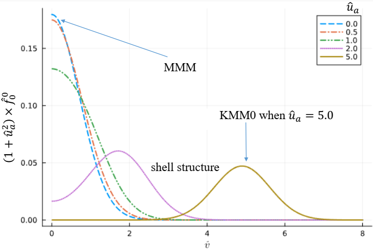
Figure 1: Illustration of the velocity distribution functions multiplied by a factor $(1+\hat{u}_{a}^{2})$ for $N_{k_{a}}\equiv 1$ and various normalized average velocity $\hat{u}_{a}$.

The velocity shell structureMin and Liu (2015) is a typical characteristic feature for $\alpha$ particle distribution functionGorelenkov et al. (2014) in burning plasma. When $\sum_{r}(|\hat{u}_{a_{r}}|^{2})$ in KMM0 (40) is greater than zero, we call that the distribution function described by KMM0 has velocity shell structure. This structure can be observed in Fig. 1, particularly when $\hat{u}_{a}>1$.

When there is no shell structure in velocity space for the distribution function, we can simplify Eq. (40) using $\hat{u}_{a_{r}}\equiv 0,\forall r$ as

$$\hat{f}_{l}^{0}\left(\hat{v},t\right) = \frac{\delta_{l}^{0}}{\pi^{3/2}}\sum_{r=1}^{N_{k_{a}}}\left[\frac{\hat{n}_{a_{r}}}{\hat{v}_{{ath}_{r}}^{3}}\exp{\left(-\frac{\hat{v}^{2}}{\hat{v}_{{ath}_{r}}^{2}}\right)}\right]\leavevmode\nobreak\ .$$ (43)

The Maxwellian mixture model (MMM), denoted by Eq. (43), represents a shell-less distribution, which indicates that the plasma is in a shell-less quasi-equilibrium state. Fig. 1 illustrates velocity distribution functions described by KMM0 (including MMM) as a function of $\hat{v}$, along with various normalized average velocity $\hat{u}_{a}$ when $\hat{v}_{{ath}_{r}}\equiv 1$. To examine the details of cases where $\hat{u}_{a}>1$, the distribution function is multiplied by a factor of $(1+\hat{u}_{a}^{2})$. The convergence of KMM0 and MMM can be proved based on Wiener’s Tauberian theoremWiener (1932); Mandrekar (1995); Vladimirov et al. (1988); Korevaar (2004). The proof is provided in Appendix A.

The above models are under the finitely distinguishable independentTeicher (1963); Yakowitz and Spragins (1968) features assumption. This assumption posits that given indistinguishable condition (42), a finite-volume, finite-density, finite-temperature, and finite-component fully ionized plasma system has a finite number of distinguishable independent characteristics. This assumption indicates that $N_{k_{a}}$ is a finite-size number in KMM0 (40).

Under this assumption, substituting Eq. (40) into Eq. (25), and simplifying the result yields the characteristic parameter equation when velocity space of the system exhibits spherical symmetry, namely:

$${\mathcal{M}}{{}_{j,l}^{0}}\left(t\right)=\delta_{l}^{0}{C_{M}}_{j}^{0}\rho_{a}v_{ath}^{j}\sum_{r=1}^{N_{k_{a}}}\hat{n}_{a_{r}}\hat{v}_{{ath}_{r}}^{j}\left[1+\sum_{k=1}^{j/2}C_{j,0}^{k}\left(\frac{\hat{u}_{a_{s}}}{\hat{v}_{{ath}_{r}}}\right)^{2k}\right]\leavevmode\nobreak\ .$$ (44)

The coefficient

$${C_{M}}_{j}^{0} = \frac{(j+1)!!}{2^{j/2}}$$ (45)

and

$$C_{j,0}^{k} = 2^{k}\frac{C_{(j-k)/2}^{k}}{(2k+1)!!},$$ (46)

where $C_{(j-k)/2}^{k}$ is the binomial coefficient. Similarly, Substituting Eq. (43) into Eq. (25) gives:

$${\mathcal{M}}{{}_{j,l}^{0}}\left(t\right) = \delta_{l}^{0}{C_{M}}_{j}^{0}\rho_{a}\left(v_{ath}\right)^{j}\sum_{s=1}^{N_{k_{a}}}\hat{n}_{a_{r}}\left(\hat{v}_{{ath}_{r}}\right)^{j}\leavevmode\nobreak\ .$$ (47)

In particular, when $j=2$, we obtain:

$$\mathcal{M}_{2,0}^{0}\left(t\right) = 2K_{a}\leavevmode\nobreak\ .$$ (48)

Generally, the Eq. (44) typically encompasses a total of $3N_{k_{a}}$ unidentified parameters and $2N_{k_{a}}$ unidentified parameters in Eq. (47).

The characteristic parameter equation (44) are a set of nonlinear algebraic equations. If we have knowledge of $3N_{k_{a}}$ kinetic moments ${\mathcal{M}}{{}_{j,0}^{0}}$, solving the well-posed characteristic parameter equations can provide us with all the characteristic parameters in Eq. (40) or Eq. (43). The KMM0 (similar to MMM) method is also noteworthy for its ability to achieve moment convergence.

Similarly, the normalized amplitudes of background distribution function can be approximated as:

$$\hat{F}_{L}^{0}\left(\hat{v}_{b},t\right) = \delta_{L}^{0}\frac{\sqrt{2\pi}}{\pi^{3/2}}\sum_{s=1}^{N_{k_{b}}}\hat{n}_{b_{s}}\mathcal{K}_{0}\left(\hat{v};\hat{u}_{b_{s}},\hat{v}_{{bth}_{s}}\right)\leavevmode\nobreak\ .$$ (49)

III.3 Kinetic moment-closed model based on MMM

The analytical expression of the $(j,l,0)^{th}$-order normalized kinetic dissipative force (35) can be obtained by substituting Eqs. (40)-(43) and  (49) into Eq. (21), and then applying Eq. (29). When the velocity space exhibits spherical symmetry without shell structure, which means $\hat{u}_{a_{r}}\equiv 0,\forall r$ and $\hat{u}_{b_{s}}\equiv 0,\forall s$, this expression will be:

$$\begin{aligned} {{\hat{\mathcal{R}}}{{}_{ab}}}{{}_{j,l}^{0}}\left(t\right)\ =&\ \delta_{l}^{0}\frac{2}{\pi^{2}}{\Gamma}\left(\frac{3+j}{2}\right)\sum_{s=1}^{N_{k_{b}}}\hat{n}_{b_{s}}\sum_{r=1}^{N_{k_{a}}}\hat{n}_{a_{r}}\frac{1}{\hat{v}_{{ath}_{r}}^{7}}\left[m_{M}\hat{v}_{{ath}_{r}}\left(\frac{1+v_{abth}^{2}}{\hat{v}_{{ath}_{r}}^{2}}\right)^{-(3+j)/2}-\right.\\ &\left.\left(\hat{v}_{{ath}_{r}}\right)^{3+j}\frac{\hat{v}_{{bth}_{s}}^{2}-m_{M}v_{abth}^{2}\hat{v}_{{ath}_{r}}^{2}}{v_{abth}^{4}\hat{v}_{{bth}_{s}}}\mathrm{{}_{2}F_{1}}\left(\frac{1}{2},\frac{3+j}{2},\frac{3}{2},-\frac{v_{abth}^{2}\hat{v}_{{ath}_{r}}^{2}}{\hat{v}_{{bth}_{s}}^{2}}\right)+\ \right.\\ &\left.\left(m_{M}-1-\frac{\hat{v}_{{bth}_{s}}}{v_{abth}^{4}}\right)\frac{\hat{v}_{{ath}_{r}}^{2}}{v_{abth}^{2}\hat{v}_{{bth}_{s}}}\left(\frac{1}{\hat{v}_{{ath}_{r}}^{2}}+\frac{v_{abth}^{2}}{\hat{v}_{{bth}_{s}}^{2}}\right)^{-(3+j)/2}\right],\quad j\geq-2,\end{aligned}$$ (50)

where $\mathrm{{}_{2}F_{1}}(a,b,c,z)$ represents the Gauss hypergeometric2F1Arfken and Pan (1971) function of the variable $z$ and parameter $v_{abth}=v_{ath}/v_{bth}$. Similarly, the normalized dissipative force arising from the self-collision process can be expressed as:

$$\begin{aligned} {{\hat{\mathcal{R}}}{{}_{aa}}}{{}_{j,l}^{0}}\left(t\right)\ =&\ \delta_{l}^{0}\frac{2}{\pi^{2}}{\Gamma}\left(\frac{3+j}{2}\right)\sum_{s=1}^{N_{k_{a}}}\hat{n}_{a_{s}}\sum_{r=s}^{N_{k_{a}}}\hat{n}_{a_{r}}\frac{1}{\hat{v}_{{ath}_{r}}^{7}}\frac{1}{\hat{v}_{{ath}_{s}}^{7}}s\left[2^{-(3+j)/2}(\hat{v}_{{ath}_{r}})^{4+j}-\right.\\ &\left.\left(\hat{v}_{{ath}_{r}}\right)^{3+j}\frac{\hat{v}_{{ath}_{s}}^{2}-\hat{v}_{{ath}_{r}}^{2}}{\hat{v}_{{ath}_{s}}}\mathrm{{}_{2}F_{1}}\left(\frac{1}{2},\frac{3+j}{2},\frac{3}{2},-\frac{\hat{v}_{{ath}_{r}}^{2}}{\hat{v}_{{ath}_{s}}^{2}}\right)-\right.\\ &\left.\hat{v}_{{ath}_{s}}\left(\frac{1}{\hat{v}_{{ath}_{r}}^{2}}+\frac{1}{\hat{v}_{{ath}_{s}}^{2}}\right)^{-(3+j)/2}\right],\quad j\geq-2\leavevmode\nobreak\ .\end{aligned}$$ (51)

The combination of Eqs. (43),  (47),  (33)-(35) and Eqs. (50)-(51) constitutes a set of nonlinear equations for the situation when velocity space exhibits spherical symmetry without shell structure, which will be named as kinetic moment-closed model. Kinetic moment-closed model for homogeneous plasma is a relaxation model. The flowchart to solve this nonlinear model is given in Appendix B.

Specially, the transport equations of mass density (36), momentum (37) and energy (38) of spices $a$ will be:

$$\frac{\partial}{\partial t}\rho_{a}\left(t\right) = \frac{\partial}{\partial t}I_{a}\left(t\right)\ =\ 0$$ (52)

and

$$\frac{\partial}{\partial t}K_{a}\left(t\right)=\frac{3}{4}\rho_{a}v_{ath}^{2}\left(\frac{n_{b}}{v_{bth}^{3}}\Gamma_{ab}{\hat{\mathcal{R}}}{{}_{ab}}_{2,0}^{0}+\frac{n_{a}}{v_{ath}^{3}}\Gamma_{aa}{\hat{\mathcal{R}}}{{}_{aa}}_{2,0}^{0}\right)\leavevmode\nobreak\ .$$ (53)

As pointed out in Sec. III.3.2 that the traditional Braginskii modelBraginskii (1958); Taitano et al. (2015) is a special case of our relaxation model, which computes the evolution of plasma system based on Maxwellian model. Compared to Braginskii model, there are three advantages for our relaxation model: I) Relaxation model explicitly gives the analytical forms of nonlinear kinetic dissipative closure relations (35) based on arbitrary order kinetic dissipative forces (50)-(51). II) Relaxation model is based on the conserved moments and high-order kinetic moments to describe the system evolution (33), rather than just based on the conserved moments (mass and energy) (61) in the Braginskii model. Therefore, relaxation model is more suitable for constructing numerical algorithms with high-order moment convergence. III) Relaxation model adaptively determines the optimal number of sub-distribution functions in each step, based on the characteristic parameter equation (44).

III.3.1 Special case: Two-temperature thermal equilibrium model

The numbers of sub-distribution are both equal to 1, $N_{k_{a}}=N_{k_{b}}\equiv 1$, when the two species are in thermal equilibrium at different temperatures. Consequently, $\hat{n}_{a_{r}}=\hat{n}_{b_{s}}\equiv 1$ and $\hat{v}_{{ath}_{r}}=\hat{v}_{{bth}_{s}}\equiv 1$, leading to the simplification of Eq. (50), reads:

$${\hat{\mathcal{R}}}{{}_{ab}}_{j,0}^{0}\left(t\right)=\left\{\begin{aligned} &0,\quad j=0,\\ &\frac{C_{j}^{R}}{2}\left[\left(\frac{1}{v_{abth}}+v_{abth}\right)\arctan(v_{abth})-1\right],\quad j=1,\\ &C_{j}^{R}\left[1+\sum_{k=2}^{j/2}(v_{abth})^{2k}\boldsymbol{c}_{j}[k]\right],\quad j\in 2\mathbb{N}^{+},\\ &C_{j}^{R}\left[\mathrm{{}_{2}F_{1}}\left(-\frac{j}{2},1,\frac{3}{2},-v_{abth}^{2}\right)-1\right],\quad j\in 2\mathbb{N}^{+}+1\leavevmode\nobreak\ .\\ \end{aligned}\right.$$ (54)

Operator $\boldsymbol{c}_{j}\left[k\right]$ in Eq. (54) represents the $k^{th}$ element of the vector $\boldsymbol{c}_{j}$, and satisfies the following recursive relationship:

$$\boldsymbol{c}_{j}[k]=\frac{j-2k}{2k+3}\boldsymbol{c}_{j}[k-1],\ \boldsymbol{c}_{j}[1]=1,\ 2\leq k\leq j/2\leavevmode\nobreak\ .$$ (55)

Parameter

$$C_{j}^{R}=\left\{\begin{aligned} &\frac{1}{\pi^{3/2}}\frac{j(j+1)!!}{3\sqrt{2^{j}}}\frac{1}{v_{abth}^{2}}\frac{1-m_{M}v_{abth}^{2}}{\sqrt{\left(1+v_{abth}^{2}\right)^{j+1}}},j\in 2\mathbb{N}^{+},\\ &\frac{2}{\pi^{2}}\frac{\left(j/2+1/2\right)!}{v_{abth}^{4}}\frac{1-m_{M}v_{abth}^{2}}{\sqrt{\left(1+v_{abth}^{2}\right)^{j+1}}},j\in 2\mathbb{N}^{+}+1\leavevmode\nobreak\ .\\ \end{aligned}\right.$$ (56)

Eq. (54) reveals that the arbitrary order normalized kinetic dissipative force solely depends on $m_{M}$ and $v_{abth}$, indicating that the high-order normalized kinetic dissipative force is not an independent quantity when the two species are in thermal equilibrium respectively.

Similarly, Eq. (51) reduces to be:

$${{\hat{\mathcal{R}}}{{}_{aa}}}{{}_{j,0}^{0}}\left(t\right) \equiv 0,\quad j\geq-2\leavevmode\nobreak\ .$$ (57)

In other words, any order normalized kinetic moments during self-collision process remain constant over time when the distribution function of species $a$ is in thermodynamic equilibrium. In this case, the transport equation (33) will be:

$$\frac{\partial}{\partial t}{\mathcal{M}}{{}_{j,l}^{0}}\left(t\right) = \delta_{l}^{0}\rho_{a}\left(v_{ath}\right)^{j}\frac{n_{b}}{v_{bth}^{3}}\Gamma_{ab}{{\hat{\mathcal{R}}}{{}_{ab}}}{{}_{j,l}^{0}},$$ (58)

where function ${{\hat{\mathcal{R}}}{{}_{ab}}}{{}_{j,l}^{0}}$ satisfies Eq. (54).

III.3.2 Special case: Braginskii model

In particular, the $(2,0,0)^{th}$-order transport equation, when the two species are in thermodynamic equilibrium at different temperatures, will be:

$$\frac{\partial}{\partial t}\mathcal{M}_{2,0}^{0}\left(t\right)=\frac{\rho_{a}v_{ath}^{2}}{\pi^{3/2}}\frac{n_{b}}{v_{bth}^{3}}\Gamma_{ab}\frac{1-m_{M}v_{abth}^{2}}{v_{abth}^{2}\sqrt{\left(1+v_{abth}^{2}\right)^{3}}}\leavevmode\nobreak\ .$$ (59)

Substituting Eq. (48) into the above equation yields:

$$\frac{\partial}{\partial t}T_{a}\left(t\right)=\frac{1}{3}\frac{m_{a}v_{ath}^{2}}{\pi^{3/2}}\frac{n_{b}}{v_{bth}^{3}}\Gamma_{ab}\frac{1-m_{M}v_{abth}^{2}}{v_{abth}^{2}\sqrt{\left(1+v_{abth}^{2}\right)^{3}}}\leavevmode\nobreak\ .$$ (60)

The above equation can be simplified and expressed as follows:

$$\frac{\partial}{\partial t}T_{a}\left(t\right)=-\nu_{T}^{ab}\left(T_{a}-T_{b}\right)\leavevmode\nobreak\ .$$ (61)

Eq. (61) is the classical Braginskii modelBraginskii (1958); Taitano et al. (2015). The characteristic frequency of temperature relaxation is consistent with the result obtained by HubaHuba (2011), which can be expressed as:

$$\nu_{T}^{ab}=\frac{1}{3}\frac{1}{\sqrt{2\pi}}\left(\frac{q_{e}^{2}}{4\pi\varepsilon_{0}}\right)^{2}\frac{\sqrt{m_{a}m_{b}}\left(Z_{a}Z_{b}\right)^{2}n_{b}}{\left(m_{a}T_{b}+m_{b}T_{a}\right)^{3/2}}\ln{\Lambda_{ab}}\leavevmode\nobreak\ .$$ (62)

In above equation, $q_{e}$ is the charge of the positron; $Z_{a}$ and $Z_{b}$ are the particle charge number of species $a$ and $b$, respectively.

III.3.3 Special case: Thermodynamic equilibrium model

Furthermore, in the state of thermodynamic equilibrium for the plasma system, where the numbers of sub-distributions are both equal to 1 and both species have the same temperature ($T_{a}=T_{b}$, especially when $m_{M}=v_{abth}=1$), it follows that the factor in Eq. (56) becomes $1-m_{M}v_{abth}^{2}\equiv 0$. Consequently, Eq. (54) can be expressed as follows:

$${{\hat{\mathcal{R}}}{{}_{ab}}}{{}_{j,0}^{0}}\left(t\right) = 0,\quad\forall j\leavevmode\nobreak\ .$$ (63)

Substituting Eq. (63) into Eq. (58) yields the transport equation for homogeneous plasma system is in thermal equilibrium, reads:

$$\frac{\partial}{\partial t}{\mathcal{M}}{{}_{j,0}^{0}}\left(t\right) \equiv 0,\quad\forall j\leavevmode\nobreak\ .$$ (64)

In other words, if both species are in thermodynamic equilibrium and have the same temperature during Coulomb collision process, any order of the system’s kinetic moment does not spontaneously change with time.

IV Conclusion

It has been demonstrated that a relaxation model is obtained when the velocity space exhibits spherical symmetry. This model comprises a set of transport equations of arbitrary order (include density, momentum, and energy) based on Maxwellian mixture model. These results are typically presented in closed form in term of Gauss hypergeometric2F1 functions. Furthermore, it has been demonstrated that our relaxation model encompasses specific instances such as the two-temperature thermal equilibrium model, Braginskii model, and thermodynamic equilibrium model.

It is important to note that our article focuses on proposing a mixture model based on the finitely distinguishable independent feature hypothesis rather than traditionally employed near-equilibrium hypothesis. We have derived the relaxation model for a two-species plasma with spherically symmetric velocity space using FPRS collision operator. The results accurately capture both near-equilibrium and far-from-equilibrium states for spherically symmetric plasma system. These findings will serve as valuable benchmarks for nonlinear statistical physics applications such as fusion plasma and solar plasma. In our future research, we aim to expand these findings to encompass scenarios in the general velocity space, including those involving axisymmetric systems.

V Acknowledgments

We would like to thank Yifeng Zheng, Zhihui Zou, Jian Zheng, Zhe Gao and Mengping Zhang for useful discussions. This work is supported by the Strategic Priority Research Program of the Chinese Academy of Sciences (Grant No. XDB0500302)

Appendix A Convergence of KMM0 and MMM

Convergence of KMM0 and MMM can be proved based on the Wiener’s Tauberian theorem. Wiener’s Tauberian theorem is a set of important theorems about smooth function approximation that was proposed by Norbert Wiener in 1932 Wiener (1932), which will be quoted as follows:

Theorem A. 1

(Wiener’s Tauberian theorem)

Let $f\in L^{1}(\mathbb{R})$ be an integrable function. The span of translations $g_{a}(x)=g(x+a)$ is dense in $L^{1}(\mathbb{R})$ if and only if the Fourier transform of function $f$ has no real zeros.

The Fourier transform of Gaussian function is still a Gaussian function. Therefore, the Gaussian function is obviously a dense function in the Euclidean space. Gaussian function serves as a commonly employed non-orthogonal basis for two primary reasons: Firstly, many natural statistical systems are independent and identically distributed systems that often adhere to the central limit theorem Rosenblatt (1956); Secondly, Gaussian functions offer computational simplicity. By selecting the basis $g(v)$ as a Gaussian function to approximate the distribution function $f(v)$, i.e., $F(v)=\sum_{s=1}^{N}w_{s}g(v+c_{s})$, where $w_{s}$ is the weight of basis function. This form represents the one-dimensional Gaussian mixture model Banerjee et al. (2013) (GMM) with identical expectation.

GMM with different expectations and deviations is represented by approximating the function $f(v)$ with a series of scaled and translated Gaussian functions, $g\left[\left(v+c_{s,k}\right)/\sigma_{s,k}\right]$. With $N$ expectations and $N$ deviations, this approximation can be expressed as:

$$F(v)=\sum_{k=1}^{N}\sum_{k=1}^{N}w_{s,k}g\left[\left(v+c_{s,k}\right)/\sigma_{s,k}\right]\leavevmode\nobreak\ .$$ (65)

Above equation consists of a total of $N\times N$ Gaussian functions, which can be reduced by utilizing optimization algorithms, such as the expectation-maximizationWynne et al. (2021) (EM) method. After obtaining an optimized set of parameters $\{w_{s,k},c_{s,k},\sigma_{s,k}\}$ where $s=k$, Eq. (65) can be expressed as:

$$F(v)=\sum_{k=1}^{N}w_{k}g\left[\left(v+c_{k}\right)/\sigma_{k}\right]\leavevmode\nobreak\ .$$ (66)

Specifically, when all deviations are zero ($c_{k}\equiv 0,\forall k$), Eq. (66) will be:

$$F(v)=\sum_{k=1}^{N}w_{k}g\left(v/\sigma_{k}\right)\leavevmode\nobreak\ .$$ (67)

Eq. (67) is the form of MMM (43) given in Sec. III.2. Function $\mathcal{K}_{0}$ (41) is the form of Gaussian function in spherical coordinate system when the velocity space is spherically symmetric, which can be obtain by employing the spherical harmonic expansionArfken and Pan (1971). Hence, KMM0 (40) will be convergent when the velocity space exhibits spherical symmetry.

Appendix B Flowchart to solve the relaxation model based on MMM

The relaxation model based on MMM, described in detail in Sec. III.3, generally consists of a set of nonlinear equations that can only be solved numerically. In this paper, we just present the flowchart to solve these nonlinear equations, which is provided in Fig. 2. The transport equation (33) can be solved by a Runge-Kutta solver, i.e., trapezoidalRackauckas and Nie (2017) scheme which is a second-order implicit method.

Figure 2: Flowchart of the kinetic moment-closed model for plasma when velocity space exhibits spherical symmetry without shell structure

References

- Boltzmann (1872) V. L. Boltzmann, Wissenschaftliche Abhandlungen (1872).
- Chen (1984) F. F. Chen, Introduction to Plasma Physics and Controlled Fusion Volume 1: Plasma Physics, Second Edition (Springer International Publishing, 1984).
- Mintzer (1965) D. Mintzer, Physics of Fluids 8, 1076 (1965).
- Grad (1949) H. Grad, Communications on Pure and Applied Mathematics 2, 331 (1949).
- MacDonald et al. (1957) W. M. MacDonald, M. N. Rosenbluth, and W. Chuck, Physical Review 107, 350 (1957).
- Tanenbaum (1967) B. S. Tanenbaum, Plasma physics (McGraw Hill, 1967).
- Chapman (1916) S. Chapman, Proceedings of the Royal Society of London. Series A, Containing Papers of a Mathematical and Physical Character 93, 1 (1916).
- Chapman and Cowling (1953) S. Chapman and T. G. Cowling, The Mathematical Theory of Non-Uniform Gases (Cambridge University Press, 1953).
- Burnett (1935) D. Burnett, Proceedings of the London Mathematical Society s2-39, 385 (1935).
- Schunk (1977) R. W. Schunk, Reviews of Geophysics 15, 429 (1977).
- Teicher (1963) H. Teicher, Source: The Annals of Mathematical Statistics 34, 1265 (1963).
- Yakowitz and Spragins (1968) S. J. Yakowitz and J. D. Spragins, The Annals of Mathematical Statistics 39, 209 (1968).
- Shkarofsky (1963) I. P. Shkarofsky, Canadian Journal of Physics 41, 1753 (1963).
- Shkarofsky et al. (1967) I. P. Shkarofsky, T. W. Johnston, M. P. Bachynski, and J. L. Hirshfield, American Journal of Physics 35, 551 (1967).
- Huba (2011) J. D. Huba, NRL PLASMA FORMULARY (NRL, 2011) pp. 1–71.
- Bell et al. (2006) A. R. Bell, A. P. Robinson, M. Sherlock, R. J. Kingham, and W. Rozmus, Plasma Physics and Controlled Fusion 48 (2006), 10.1088/0741-3335/48/3/R01.
- Shkarofsky (1997) I. P. Shkarofsky, Physics of Plasmas 4, 2464 (1997).
- Min and Liu (2015) K. Min and K. Liu, Journal of Geophysical Research: Space Physics 120, 2739 (2015).
- Gorelenkov et al. (2014) N. Gorelenkov, S. Pinches, and K. Toi, Nuclear Fusion 54, 125001 (2014).
- Wiener (1932) N. Wiener, The Annals of Mathematics 33, 1 (1932).
- Mandrekar (1995) V. Mandrekar, NOTICES OF THE AMS (1995).
- Vladimirov et al. (1988) V. S. Vladimirov, Y. N. Drozzinov, and B. I. Zavialov, Tauberian Theorems for Generalized Functions (Springer Netherlands, 1988).
- Korevaar (2004) J. Korevaar, Tauberian Theory, Vol. 329 (Springer Berlin Heidelberg, 2004) p. 1.
- Arfken and Pan (1971) G. Arfken and Y. K. Pan, American Journal of Physics 39, 461 (1971).
- Braginskii (1958) S. I. Braginskii, J. Exptl. Theoret. Phys. (U.S.S.R.) 6, 459 (1958).
- Taitano et al. (2015) W. T. Taitano, L. Chacón, A. N. Simakov, and K. Molvig, Journal of Computational Physics 297, 357 (2015).
- Rosenblatt (1956) M. Rosenblatt, Proceedings of the National Academy of Sciences 42, 43 (1956).
- Banerjee et al. (2013) A. Banerjee, D. B. Dunson, and S. T. Tokdar, Biometrika 100, 75 (2013).
- Wynne et al. (2021) G. Wynne, F.-X. Briol, and M. Girolami, “Convergence guarantees for gaussian process means with misspecified likelihoods and smoothness,” (2021).
- Rackauckas and Nie (2017) C. Rackauckas and Q. Nie, Journal of Open Research Software 5, 15 (2017).