Deep Reinforcement Learning for Dynamic Order Picking in Warehouse Operations

Abstract

Order picking is a crucial operation in warehouses that significantly impacts overall efficiency and profitability. This study addresses the dynamic order picking problem, a significant concern in modern warehouse management where real-time adaptation to fluctuating order arrivals and efficient picker routing are crucial. Traditional methods, often assuming fixed order sets, fall short in this dynamic environment. We utilize Deep Reinforcement Learning (DRL) as a solution methodology to handle the inherent uncertainties in customer demands. We focus on a single-block warehouse with an autonomous picking device, eliminating human behavioral factors. Our DRL framework enables the dynamic optimization of picker routes, significantly reducing order throughput times, especially under high order arrival rates. Experiments demonstrate a substantial decrease in order throughput time and unfulfilled orders compared to benchmark algorithms. We further investigate integrating a hyperparameter in the reward function that allows for flexible balancing between distance traveled and order completion time. Finally, we demonstrate the robustness of our DRL model for out-of-sample test instances.

Key words: Dynamic order picking, warehouse management, deep reinforcement learning, routing

1 Introduction

Order picking, the process of retrieving specific items from warehouse storage to fulfill customer orders, is a labor-intensive and time-consuming operation. Order pickers traverse the warehouse, collecting items from various locations before delivering them to a designated depot. Notably, order picking can constitute about 50% of the total order processing time (Charkhgard and Savelsbergh, 2015; Silva et al., 2020). Recent growth in e-commerce, coupled with heightened customer expectations for fast delivery and increased market competition, has escalated the demand for rapid order fulfillment (Marchet et al., 2015; Van Gils et al., 2018; Rasmi et al., 2022). Efficient order picking, which necessitates solving a routing problem, is crucial for several reasons. It directly enhances operational efficiency, leading to increased order throughput within the warehouse and improved customer satisfaction (Giannikas et al., 2017). Additionally, streamlining the picking process translates to cost reductions for the business.

In modern warehouse operations, the ability to accurately forecast demand and dynamically adjust order picking decisions is paramount (Lu et al., 2016; Dauod and Won, 2022). However, the existing literature predominantly focuses on exact and heuristic methods that assume a fixed set of orders is known in advance. While this approach is suitable for static scenarios, it often fails to effectively address the dynamic nature of real-world warehouse operations. To overcome these challenges, a dynamic and adaptive approach to demand forecasting and picker routing is essential. This would enable warehouses to respond swiftly to real-time order arrivals, optimizing routing decisions, minimizing operational costs, and maximizing overall efficiency.

Our research investigates picker-to-parts systems within single-block warehouses, focusing on how an autonomous picker navigates the aisles to retrieve items. This focus aligns with the growing trend of warehouse automation (Roy et al., 2019; Winkelhaus et al., 2021), and we assume the picking device flawlessly execute recommended routing decisions, thereby eliminating behavioral factors associated with human pickers. We demonstrate that a dynamic, single-picker order picking method can substantially reduce picking time in this setting. Our study serves as a foundation for future research to explore the complexities of dynamic order picking in multi-block warehouses with multiple coordinated pickers.

We employ a Deep Reinforcement Learning (DRL) framework for addressing the dynamic order picking problem due to its inherent ability to handle sequential decision-making under uncertainty. This approach is particularly well-suited for the real-world warehouse environment (Begnardi et al., 2024), characterized by the constantly changing nature of order arrivals, item locations, picker location, and picker availability. By leveraging DRL’s capability to learn and adapt in real-time, and forecast order arrivals to optimize picker routes dynamically, we can significantly improve warehouse efficiency and throughput. We demonstrate that traditional deep neural network architectures are sufficient to achieve this goal, as opposed to more complex state-of-the-art DRL models, which require longer training times or heavier computational resources.

Our experiments demonstrate that as order arrival rates increase, relying solely on the shortest-distance for order picking becomes inefficient. In scenarios with high order frequencies, the policies learned by our DRL agent substantially enhances the order fulfillment efficiency. For example, when orders follow a Poisson process with an arrival rate ($\lambda$) of 0.09, our approach reduces order throughput time by a substantial 420% compared to existing benchmark algorithms. Our approach maintains an unfulfilled order rate of approximately 2% within the work shift, while the benchmark algorithms result in up to 18% of orders remaining unfulfilled. Additionally, we demonstrate that incorporating a hyperparameter ($\alpha$) into the reward function allows us to effectively balance the trade-off between distance traveled and order throughput times, aligning with the preferences of decision-makers.

The remainder of this paper is organized as follows. Section 2 reviews relevant literature, examining various optimization approaches for order picking and applications of deep reinforcement learning in warehouse operations. In Section 3, we formally describe the problem addressed in this study. Section 4 details our proposed solution methodology and the neural network architecture employed. Section 5 presents a series of computational experiments designed to evaluate the effectiveness of our approach against existing benchmark algorithms. We also analyze the robustness of our model when confronted with out-of-sample instances. Finally, Section 6 summarizes our findings with concluding remarks, and proposes potential avenues for future research in this domain.

2 Literature Review

In this section, we first review the traditional optimization approaches for order picker routing in warehouses. We then discuss the application of DRL in addressing various warehouse operational challenges, demonstrating its potential for intelligent decision-making in complex environments. Finally, we identify a critical research gap within the dynamic order picking literature, highlighting the need for our proposed DRL-based approach.

2.1 Optimization Approaches for Order Picking Routing

Numerous methods have been proposed in the literature for order picker routing. However, most methods focus on static problem scenarios. A notable contribution for single-picker routing in single-block warehouses is Ratliff and Rosenthal (1983), who developed an efficient algorithm leveraging the graph-based structure of order storage locations in the warehouse. This algorithm has been extended to accommodate different warehouse layouts, including two-block (Roodbergen and De Koster, 2001), fish-bone (Çelk and Süral, 2014), and chevron (Masae et al., 2020b) configurations. The mathematical formulations for the same problem are presented in Scholz et al. (2016) and Pansart et al. (2018), offering advantages over the standard Traveling Salesperson Problem (TSP) solvers by utilizing the warehouse structure properties to eliminate redundant possibilities inherent in the TSP. However, these approaches are primarily designed for static environments and lack the flexibility to accommodate dynamic order arrivals, a common occurrence in real-world operations. Furthermore, practical implementation often necessitates an order batching policy due to picker capacity constraints. Lu et al. (2016) addressed these limitations by employing a first-come-first-served order batching policy and extending the static algorithm to dynamic scenarios. By utilizing this interventionist routing approach, the authors demonstrate a significant reduction in average order completion times compared to both heuristics and the static exact algorithm.

Heuristic algorithms are a popular focus in warehouse operations research due to their simplicity and ease of implementation. For example, the S-shape heuristic, where pickers traverse aisles in an S-shape curve, offers a straightforward routing policy. Hall (1993) provides a comparative analysis of various heuristic routing methods based on the number of pick locations within an aisle. The largest gap heuristic generally outperforms others when the pick list is small. However, the inherent nature of heuristic algorithms often leads to suboptimal decisions, potentially impacting overall system efficiency. Lu et al. (2016) demonstrated that their dynamic programming algorithm outperforms the largest gap heuristic in terms of both order completion time and total travel distance.

Order batching is a critical strategy that can significantly reduce the distance traveled by order pickers (De Koster et al., 2007; Henn, 2012; Muter and Öncan, 2022). However, most studies focus on either order batching or routing strategies, often employing simplistic approaches for the other aspect. Scholz and Wäscher (2017) introduced an iterated search heuristic to address the combined problem of order batching and picker routing. Their approach demonstrated better performance compared to other common methods, highlighting the advantages of integrating these two warehouse optimization problems. Recent research has seen a growing interest in dynamic pick list updating, notably in Dauod and Won (2022) and Yang et al. (2021). Due to limitations in scope, we benchmark our proposed method against Lu et al. (2016), rather than conducting a comprehensive comparison with other heuristics. Importantly, our proposed approach is dynamic and produces decisions almost instantaneously during testing, while the neighborhood searches involved in heuristics are time-consuming, leading to cumulative wait times in a dynamic order picking scenario.

For a more comprehensive literature review on order picker routing, including a detailed overview of various operational procedures, readers may refer to De Koster et al. (2007), Van Gils et al. (2018), and Masae et al. (2020a).

2.2 Deep Reinforcement Learning for Warehouse Operations

Deep Reinforcement Learning (DRL) has garnered increasing attention in the warehousing domain, with recent studies primarily focusing on order batching and assignment problems. Cals et al. (2021) pioneered DRL in warehousing by addressing the order batching and sequencing problem, aiming to minimize tardy orders. Later, Beeks et al. (2022) extended this method to a multi-objective domain, considering picking costs and analyzing the trade-off between order tardiness and picker efficiency. Li et al. (2019) proposed a DRL architecture for assigning orders to autonomous robots in a warehouse to reduce makespan in the event of traffic conflicts. Notably, these methods do not directly address optimal picker routing with the objective of minimizing travel distance or order completion times. Additionally, some studies utilize DRL for warehouse inventory management (Kaynov et al., 2024; Tian et al., 2024).

Dunn et al. (2024) address the picker routing problem using a DRL approach for combinatorial optimization. Their model, utilizing an attention-based neural network, generates high-quality solutions and is particularly effective when extended to large-scale problems where exact methods may be computationally expensive. The authors demonstrate the effectiveness of their DRL model compared to the benchmark algorithm of Ratliff and Rosenthal (1983). However, this study is confined to the static problem variant. In a recent study, Begnardi et al. (2024) propose multiple graph neural network-based DRL models to solve the collaborative human-robot picking problem, formulated as an online bipartite matching problem. However, their evaluation is limited to small-scale grid-based instances with several pickers, and benchmarks are solely compared against variations of the greedy heuristic. Given the large number of pickers within their small-scale test instances, the study focuses more on the order assignment problem rather than the routing problem.

2.3 Research Gap

Our study is the first to comprehensively address the dynamic order picker routing problem using DRL, where the agent implicitly learns order batching strategies. This approach integrates order assignment and routing within the RL agent’s learning environment. The RL agent’s ability for rapid decision-making during testing is vital to prevent unnecessary delays in picker routing. We prioritize the development of a simple yet effective model for single-block warehouses and demonstrate its superior performance in minimizing order processing delays.

3 Problem Description

Consider the order-picking problem for a single picker within a rectangular warehouse. The warehouse consists of a single block with multiple parallel aisles, interconnected by two cross-aisles at the ends. Inventory storage locations are situated on either side of each aisle. Figure 1 presents a visual representation of this warehouse layout. The picker must collect the requested items from designated storage locations within the warehouse. The picker can move through the aisles to access storage locations on both sides, and we assume that there is no horizontal travel distance within an aisle. To traverse between different aisles, the picker must utilize one of the two cross-aisles. These cross-aisles do not contain any storage locations; they solely serve as pathways for movement between the aisles. Note that the picker can only enter or exist an aisle through one of the two cross-aisles.

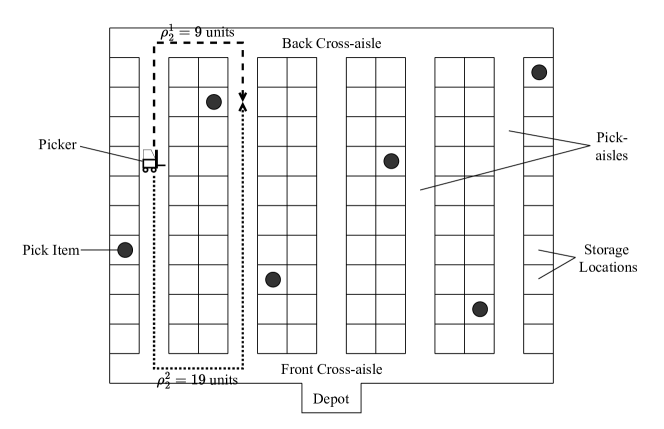
Figure 1: An illustrative example of warehouse layout for the order-picking problem

We assume that the requested items are identical in size and hold the same level of priority. The order-picking device or vehicle utilized for transporting these items has a total capacity of $K$ items. Initially, the picker starts from the depot and moves through the warehouse to collect the assigned items and delivers them to the depot, subject to the capacity constraint at all times. Figure 1 illustrates that this warehouse layout offers two alternative paths the picker can take to collect the next assigned order, denoted by the distances $\rho$. We will discuss the notation details of distances in the next section. The primary objective is to minimize the average waiting time for orders, and thereby increasing the throughput in warehouse operations. The picker route is determined based on the demand forecast, and a dynamically updated pick-list, which is adjusted based on incoming orders and the remaining orders to be collected. This optimization problem is considered over a time horizon that resembles a human picker’s work shift.

In most warehouse order-picking scenarios, customer demand fluctuates throughout a work shift, unlike static problems with pre-defined pick lists. This dynamic environment requires real-time decision-making regarding order batching and traversal routes to minimize order wait times. Reducing these wait times not only enhances customer satisfaction but also frees up resources for fulfilling additional orders, especially critical in the growing field of e-commerce. Our approach further improves order picking by incorporating implicit demand forecasting, allowing pickers to anticipate upcoming orders and optimize their paths. This contrasts with traditional methods based solely on observed order arrivals. Our findings demonstrate that this dynamic, priority-driven behavior leads to significant reductions in order wait times.

4 Methodology

In this section, we present the formulation of the real-time warehouse order picking problem. We model this problem using a finite Markov Decision Process (MDP) with discrete time steps to capture its dynamic nature. Specifically, each time step $t$ involves making a movement or a decision regarding the picker’s actions. At each step, the system state $S_{t}$ is observed, encapsulating information about both the orders, their locations in warehouse and the picker. Based on this state, an action $a_{t}$ is chosen, determining the picker’s movement direction, whether the picker should remain stationary, or if items should be released at the depot. Executing this action leads to a new system state $S_{t+1}$, from which the next action $a_{t+1}$ is determined for the subsequent time step $t+1$.

4.1 MDP Formulation

MDPs provide a structured framework for modeling decision-making processes where outcomes are influenced by both random factors and the actions of a decision maker. An MDP is defined by a five-tuple $(\textit{{S}},\textit{{A}},\textit{{P}},\textit{{R}},\gamma)$, where S represents the set of system states, A is a finite set of actions, P denotes the state transition probability, R is the immediate reward function, and $\gamma$ is the discount factor. The following are the details of the specific formulation of the MDP for our problem.

1. State: The system state at time step $t$ is denoted as $\boldsymbol{S_{t}}=(\boldsymbol{S^{p}_{t}},\boldsymbol{S^{o}_{t}})$, where $\boldsymbol{S^{p}_{t}}$ represents the picker state and $\boldsymbol{S^{o}_{t}}$ represents the state of existing orders in the warehouse.

   The picker state, $\boldsymbol{S^{p}_{t}}=(S^{H}_{t},S^{V_{1}}_{t},S^{V_{2}}_{t},S^{C}_{t})$, consists of four components: $S^{H}_{t}$, $S^{V_{1}}_{t}$, $S^{V_{2}}_{t}$, and $S^{C}_{t}$. Here, $S^{H}_{t}$ represents the horizontal position of the picker, which is the relative position of the picker with respect to cross-aisles, $S^{V_{1}}_{t}$ and $S^{V_{2}}_{t}$ represent the vertical position, which are picker’s positions with respect to pick aisles, and $S^{C}_{t}$ indicates the remaining capacity of the picker. If $S^{C}_{t}=0$, the picker is full and cannot pick up additional items; if $S^{C}_{t}=K$, the picker is empty. The horizontal state $S^{H}_{t}$ can take values of -1, 0, or 1: -1 indicates the picker is at the back cross-aisle, 1 indicates the front cross-aisle, and 0 indicates the picker is within one of the pick aisles. The exact location of the picker within a pick aisle when $S^{H}_{t}=0$ is implicitly encoded in the order state $\boldsymbol{S^{o}_{t}}$. The vertical position is determined by $S^{V_{1}}_{t}$ and $S^{V_{2}}_{t}$, which equal $2n-1$ and $2n$ when the picker is at aisle $n$. The rationale for representing each pick aisle by two consecutive indices, rather than a single index, lies in the formulation of $\boldsymbol{S^{o}_{t}}$ as a vector of size $2N$. Enhancing this consistency between the two components of the state helps in the neural network’s interpretation.
   

   The state of orders, $\boldsymbol{S^{o}_{t}}=(S^{1}_{t},S^{2}_{t},\ldots,S^{2N-1}_{t},S^{2N}_{t})$, where $N$ is the number of pick aisles in the warehouse. Each aisle $n$ is represented by $S^{2n-1}_{t}$ and $S^{2n}_{t}$. These values indicate the state of orders in each pick aisle depending on the picker’s vertical movement direction. $S^{2n-1}_{t}$ represents the value of orders if the picker moves upward in its current aisle, while $S^{2n}_{t}$ represents the value if the picker moves downward. These values are computed by summing the value of each order in the aisle divided by its distance from the picker, based on the direction of movement. The distance between the picker and an order is the smallest number of movements required for picker to reach the order in terms of the number of location storage. These states are calculated as

   $$S^{2n-1}_{t}=\displaystyle\sum_{i=1}^{L}\displaystyle\frac{n_{i}}{\rho^{1}_{i}}\mbox{ and }S^{2n}_{t}=\displaystyle\sum_{i=1}^{L}\displaystyle\frac{n_{i}}{\rho^{2}_{i}},$$

   where $L$ is the number of pick locations in each aisle, $n_{i}$ is the number of orders at pick location $i$, and $\rho^{1}_{i}$ and $\rho^{2}_{i}$ are the distances of picker to pick location $i$ when moving upward or downward, respectively.
   

   For example, consider the picker’s position and the requested items in Figure 1. We assume that the picker is empty and thus the picker state is $\boldsymbol{S^{p}_{t}}=(0,1,2,$K$)$. The distance traveled through each unit square in the figure is 1 unit, and the distance between adjacent cross-aisles is 3 units. Note that each storage location with a requested item in the figure contains only one requested item. Now, the order state can be determined as follows. For the first aisle,

   $$S^{1}_{t}=0\mbox{ and }S^{2}_{t}=\displaystyle\frac{1}{3}=0.33.$$

   Similarly, for the second aisle,

   $$S_{3}=\displaystyle\frac{1}{9}+\displaystyle\frac{1}{15}=0.18\mbox{ and }S_{4}=\displaystyle\frac{1}{13}+\displaystyle\frac{1}{19}=0.13.$$

   Thus, the order state is calculated as $\boldsymbol{S^{o}_{t}}=(0,0.33,0.18,0.13,0,0,0.06,0.04,0.10,0.08)$.
   

   This formulation implicitly captures the importance of the picker’s visiting direction for each aisle. Notably, when $S^{H}_{t}=-1$, then $S^{2n}_{t}=0$ for all aisles since the picker cannot move upward. Similarly, when $S^{H}_{t}=1$, then $S^{2n-1}_{t}=0$ for all aisles. The starting state is $\boldsymbol{S^{o}_{0}}=\boldsymbol{0}$ since there are no orders at time zero, and $\boldsymbol{S^{p}_{t}}=(1,2d-1,2d,K)$, where $d$ is the aisle where depot is located at, and $K$ is the picker capacity.

2. Action: Given the state $S_{t}$, the action $a_{t}$ determines the picker’s decision. The action $a_{t}$ can take on values from 0 to 4. Specifically, $a_{t}=0$ signifies that the picker drops off items if located at the depot, and otherwise results in no movement. Actions with values 1 and 2 correspond to moving the picker to the right and left, respectively. In this study, actions are constrained to feasible options only. For instance, when the picker is situated within a pick aisle (i.e., $S^{H}_{t}=0$), actions 1 and 2 are disallowed. Actions 3 and 4 correspond to moving the picker upward and downward, respectively. Additionally, when the picker is in the back cross-aisle (i.e., $S^{H}_{t}=-1$), action 3 is prohibited, and when the picker is in the front cross-aisle (i.e., $S^{H}_{t}=1$), action 4 is prohibited.

3. State Transition: In our MDP formulation, the state transition describes how the system evolves from one state to another based on the actions taken by the picker and the randomness involved in the order arrival. Let $\tau$ represent the smallest unit of time in which the picker can move from one storage location to another. If action $a_{t}=0$ is executed at any location other than the depot, it indicates that the picker remains stationary for $\tau$ time until the next step. Consequently, $\boldsymbol{S^{p}_{t+1}}$ will be identical to $\boldsymbol{S^{p}_{t}}$, and $\boldsymbol{S^{o}_{t+1}}$ will remain unchanged unless a new order arrives during $\tau$, in which case it will be recalculated. The number of new orders arriving within this interval depends on the order arrival rate.
   

   If action $a_{t}=0$ is executed at the depot, the picker will unload all items. Therefore, if $\boldsymbol{S^{p}_{t}}=(1,2d-1,2d,S^{C}_{t})$ and $a_{t}=0$, then $\boldsymbol{S^{p}_{t+1}}=(1,2d-1,2d,K)$ and $\boldsymbol{S^{o}_{t+1}}$ will be recalculated based on the orders arriving during the time required to unload $K-S^{C}_{t}$ items. Actions $a_{t}=1$ and $a_{t}=2$ can only be performed in cross aisles and require time proportional to the inter-aisle distance. Given $\boldsymbol{S^{p}_{t}}=(S^{H}_{t},S^{V_{1}}_{t},S^{V_{2}}_{t},S^{C}_{t})$, if $a_{t}=1$ is executed, the new state will be $\boldsymbol{S^{p}_{t+1}}=(S^{H}_{t},S^{V_{1}}_{t}+2,S^{V_{2}}_{t}+2,S^{C}_{t})$. Conversely, if $a_{t}=2$ is executed, $\boldsymbol{S^{p}_{t+1}}=(S^{H}_{t},S^{V_{1}}_{t}-2,S^{V_{2}}_{t}-2,S^{C}_{t})$.
   

   In our MDP formulation, actions 3 and 4 result in a new state under one of the following conditions: the picker reaches a cross aisle and cannot proceed further, a new order arrives altering $\boldsymbol{S^{o}_{t}}$, or the picker collects at least one item. It is assumed that the picker collects all items at a storage location before transitioning to a new state. When action $a_{t}=3$ or $a_{t}=4$ is executed, the state of orders $\boldsymbol{S^{o}_{t}}$ will change irrespective of new order arrivals due to the altered relative distance caused by the picker’s movement. For the picker state $\boldsymbol{S^{p}_{t+1}}$, $S^{H}_{t+1}$ may change based on whether the picker moves from a cross aisle to within an aisle or vice versa, but $S^{V_{1}}_{t+1}$ and $S^{V_{2}}_{t+1}$ will remain unchanged. The value of $S^{C}_{t+1}$ will depend on the number of items collected during the action.

4. Reward: The reward at time step $t$ is defined as follows:

   $$r_{t}=\begin{cases}-1&\text{if }a_{t}=0\text{ and picker not at the depot}\\ R\cdot(K-S^{C}_{t})\cdot\alpha&\text{if }a_{t}=0\text{ and picker at the depot}\\ -n^{m}_{t}+R\cdot n^{p}_{t}&\text{otherwise}\end{cases}$$

   Here, $R$ denotes the reward for picking up an item, $n^{m}_{t}$ represents the number of storage locations the picker moves during the time step, and $n^{p}_{t}$ indicates the number of items picked up by the picker. When the picker is at the depot location and $a_{t}=0$, this action implies unloading all items. The number of items in the picker is $K-S^{C}_{t}$, and $\alpha$ is a coefficient that modulates the reward for unloading items relative to picking them up. The value of $\alpha$ ranges between 0 and 1, where smaller values signify that picking up items is more valuable than unloading them at the depot, while larger values imply equal value for both actions. This parameter is designed to balance the trade-off between average time and average distance per order. It is anticipated that with smaller values of $\alpha$, the picker would attempt to maximize its capacity usage before heading towards the depot, thereby minimizing traveling distance. Conversely, with larger values of $\alpha$, the picker would prefer to unload items as soon as possible, minimizing both wait time and delivery time.

4.2 Proposed Approach

Our objective is to train a policy that aims to maximize the discounted cumulative reward $R_{t}=\sum_{k=0}^{\infty}\gamma^{k}\cdot r_{t+k}$, where $R_{t}$ is referred to as the return, and $0<\gamma<1$ is the discount factor that balances the importance between immediate and future rewards. Small values of $\gamma$ indicate that immediate actions are more significant than future actions, while larger values of $\gamma$ place greater emphasis on future rewards.

The fundamental concept behind Q-learning is that if we had access to a function $Q^{*}:\text{State}\times\text{Action}\rightarrow\mathbb{R}$, which could inform us of the expected return if we were to take a particular action in a given state, we could straightforwardly construct a policy that maximizes our rewards: $\pi^{*}=\arg\max_{a}Q^{*}(s,a)$, where $Q^{*}(s,a)=\max(E_{\pi^{*}}[R_{t}\mid s_{t}=s,a_{t}=a])$. However, due to the complexity of the environment, we do not have direct access to $Q^{*}$. Nevertheless, since neural networks are universal function approximators, we can construct a neural network and train it to approximate $Q^{*}$.

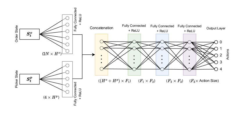
Figure 2: Proposed Deep Neural Network Architecture

4.2.1 Architecture of Deep Neural Network

The deep neural network architecture designed for this study is specifically tailored to handle the state representation and predict optimal actions for the picker in a dynamic warehouse environment. The network serves as a Q-network, approximating the action-value function $Q(s,a)$, and consists of several fully connected layers to process both the picker state and the order state separately before combining them for the final action prediction. Figure 2 provides a summary of the architecture.

The architecture is structured as follows:

• Input Layers: The input to the neural network is divided into two parts: the picker state $S^{p}_{t}$ and the order state $S^{o}_{t}$. The picker state $S^{p}_{t}$ is a four-dimensional vector represented as $(S^{H}_{t},S^{V_{1}}_{t},S^{V_{2}}_{t},S^{C}_{t})$, while the order state $S^{o}_{t}$ is a vector of size $2N$, where $N$ is the number of aisles in the warehouse.

• Processing Picker State: The picker state input $S^{p}_{t}$ is processed by the first fully connected layer, transforming the four-dimensional picker state vector into a $H^{p}$-dimensional feature vector using a ReLU activation function. This transformation helps in capturing the essential features of the picker state.

• Processing Order State: The order state input $S^{o}_{t}$ is processed by a second fully connected layer, which transforms the $2N$-dimensional order state vector into a $H^{o}$-dimensional feature vector using a ReLU activation function. This layer extracts meaningful features from the state of orders in the warehouse.

• Combining Picker and Order States: The feature vectors obtained from processing the picker state and order state are concatenated into a single vector. This combined vector with size $H^{p}+H^{o}$, integrates the information from both states, resulting in a comprehensive representation of the system state.

• Further Processing of Combined Features: The concatenated vector is then passed through a series of fully connected layers:

  • The first layer in this series has $F_{1}$ units and uses a ReLU activation function to further transform the combined feature vector.

  • The subsequent layer reduces the dimensionality to $F_{2}$ units, again using a ReLU activation function.

  • Another layer reduces the dimensionality further to $F_{3}$ units, continuing with the ReLU activation function.

• Output Layer: Finally, the output layer maps the $F_{3}$-dimensional feature vector to the action space, predicting the Q-values for each possible action. The action with the highest Q-value is then selected as the optimal action for the picker.

This deep neural network architecture effectively captures the complex interactions between the picker and the orders in the warehouse, enabling it to predict optimal actions that maximize the cumulative reward over time.

4.2.2 Training of Deep Neural Network

The training process leverages two neural networks: a policy network and a target network. The policy network guides decision-making, selecting actions based on the epsilon-greedy strategy, which balances exploration of action space and exploitation of the learned values. The target network, on the other hand, serves as a stable reference, updated periodically with the policy network’s learned parameters. To enhance the learning process, we employ the replay memory mechanism. Replay memory acts as a repository to store the agent’s experiences in the form of state transitions. During training, the DRL agent randomly samples mini-batches of transitions from the replay memory. This allows for efficient reuse of past experiences, which helps to stabilize the learning process.

The training is conducted over $N_{e}$ episodes, each comprising $N_{s}$ steps. At each step, the agent observes the current state, selects an action using the epsilon-greedy method and the policy network, and and receives a reward upon transitioning to the next state. The current state, action, next state, and reward form a transition, and is stored in the replay memory with capacity $C$. Subsequently, a randomly selected mini-batch of transitions is sampled from the memory, and the policy network undergoes one step of training based on these experiences. If the replay memory lacks sufficient transitions to form a mini-batch, the training step is skipped temporarily.

The training procedure for each mini-batch is a multi-step process. First, the states, next states, actions, and rewards within the batch are stacked for parallelization. Then, the policy network is set to training mode, while the target network enters evaluation mode. This setup allows for the computation of state-action values using the policy network, and expected state-action values using the target network. The discrepancy between these values is then used to calculate the loss, and we utilize the Huber loss function for robustness. The calculated loss is then backpropagated through the policy network, facilitating its optimization. To ensure stability, the target network is updated less frequently, specifically every $N_{\text{update}}$ steps. This update follows the soft update rule using target update weight $\tau$, where the new target network weights are updated as the weighted average of the policy network weights and the existing target network weights. This gradual update mechanism helps prevent drastic fluctuations and promotes smoother learning. The DQN training procedure is outlined in the pseudocode presented in Algorithm 1.

Algorithm 1 Training Procedure for DQN in Real-Time Warehouse Order Picking

1:Initialize policy network $\pi_{\theta}$ and target network $\pi_{\theta^{-}}$ with weights $\theta$ and $\theta^{-}=\theta$

2:Initialize replay memory $D$ with capacity $C$

3:for episode = 1 to $N_{e}$ do

4:     Initialize state $S_{0}$

5:     for t = 1 to $N_{s}$ do

6:         With probability $\epsilon$, select a random action $a_{t}$

7:         Otherwise, select $a_{t}=\arg\max_{a}Q(S_{t},a;\theta)$

8:         Execute action $a_{t}$ and observe reward $r_{t}$ and next state $S_{t+1}$

9:         Store transition $(S_{t},a_{t},r_{t},S_{t+1})$ in replay memory $D$

10:         if size of $D$ $\geq$ mini-batch size then

11:              Sample random mini-batch of transitions from $D$

12:              Set $S_{M}$, $S_{M}^{\prime}$ as states and next states in the mini-batch

13:              Set $A$ as actions, $R$ as rewards

14:              Compute $Q(S_{M},A;\theta)$

15:              Set $Q_{\text{target}}=R+\gamma\cdot\max_{a^{\prime}}Q(S_{M}^{\prime},a^{\prime};\theta^{-})$

16:              Compute loss $L=\text{HuberLoss}(Q(S_{M},A;\theta),Q_{\text{target}})$

17:              Perform gradient descent on $L$ to update $\theta$

18:         end if

19:         if $t\pmod{N_{\text{update}}}==0$ then

20:              Update target network $\theta^{-}=\tau\theta+(1-\tau)\theta^{-}$

21:         end if

22:     end for

23:end for

5 Computational Study

Experimental Settings

The warehouse layout and instance generation process employed in this study are derived from Lu et al. (2016). The warehouse configuration consists of a single block with two cross-aisles and 10 parallel aisles, each containing 15 storage locations on either side. Each aisle is 15 meters long, with 3-meter spacing between adjacent aisles. We assume that the depot is located at the end of aisle 6, adjacent to the front cross-aisle, with negligible travel time between these points. The order-picker operates at a speed of 1 meter per second, with a picking time of 5 seconds per item and an additional 1 second for an item drop-off at the depot. The picking device has a capacity ($K$) of 20 items. We assume orders arrive according to a Poisson process and conduct experiments with arrival rates ranging from 0.01 to 0.09 orders per second. For each order arrival rate, we conduct 10 independent simulation runs and report the average results to ensure reliable performance assessment. Each experiment simulates an 8-hour work shift, during which incoming orders are dynamically assigned to the picker to optimize warehouse order-picking throughput. An order is considered complete only after the picker deposits the item at the depot, and not upon retrieval from the respective storage location.

Evaluation Metrics

To evaluate the efficiency of the proposed dynamic order-picking algorithm, we employ three key metrics:

1. Average Travel Distance per Order (ATDO): The total distance traveled by an order picker during a work shift, divided by the number of completed orders.

2. Average Order Completion Time (AOCT): The average time elapsed between an order arrival at the warehouse and its final delivery at the depot by the order-picker. Our research prioritizes minimizing AOCT. By streamlining order processing, we aim to reduce customer wait times and consequently improve order fulfillment rates.

3. Percentage of Unfulfilled Orders (PUO): The percentage of orders that are not successfully completed within the work shift. A high PUO may indicate high order arrival rates, limited picking device capacity, or inefficient routing.

Traditionally, when designing order picking algorithms or strategies, more focus has been placed on the shortest path. However, as highlighted in Section 2, the primary objective in warehouse management is to minimize order throughput time. Therefore, our solution methodology prioritizes both AOCT and PUO.

5.1 Benchmark Algorithms

To evaluate our order-picker routing algorithm, we utilize two well-known benchmark studies from the literature:

1. Ratliff and Rosenthal (1983): This seminal work introduced an efficient algorithm for the static order picking problem. The order picker operates under a batching strategy, waiting for the pick list to reach the capacity of picking device, followed by a shortest tour to fulfill the orders. The authors employ a graph-based dynamic programming approach to reduce the computational complexity compared to standard TSP solution methods.

2. Lu et al. (2016): This study adapts the static order picking approach for dynamic environments, under certain assumptions. Specifically, the order picker begins a tour when incoming orders reach 25% of device capacity and can be re-routed if new orders arrive within capacity limits. Furthermore, assuming narrow cross-aisles, the picker cannot be re-routed while traveling within them. This method is referred to as the Interventionist Routing Algorithm (IRA). The authors have demonstrated the superiority of their method compared to an effective heuristic known as the largest gap heuristic.

We note that the source code for the aforementioned algorithms is unavailable. More importantly, the core of the above-mentioned studies relies on Dynamic Programming (DP) methods, which are favored for their efficacy in picker routing. However, these DP methods operate under certain assumptions, and extending them to accommodate the diverse routing scenarios found in real-world warehouse operations is not a trivial task. For instance, although picker re-routing within cross-aisles is practical and significantly impacts operational efficiency (as will be shown in the numerical results), it is assumed to be prohibited in these DP methods. Note that our proposed DRL agent automatically learns to apply cross-aisle re-routing as needed. Therefore, to replicate the results of the aforementioned studies under their assumptions, as well as to make these methods adaptable for various routing scenarios, we replace DP with a generic TSP solver in their methods to compute optimal routes. This allows for more flexible routing scenarios, such as using smaller initial pick list sizes or permitting cross-aisle re-routing. Although a generic TSP solver is slower, it does not alter the fundamental nature of the algorithms’ performance. We exclude the computational time of the generic TSP solver in our experiments. Additionally, in our computational study, we do not report any computational time, as the proposed DRL method makes decisions instantaneously at any given state. Thus, the runtime is negligible during testing, with all computational time spent during the training phase. With these considerations, we establish five baseline models for our computational study:

1. Baseline 1: The initial pick list size $k$ is set equal to the picker capacity. This replicates the static routing approach of Ratliff and Rosenthal (1983). Note that cross-aisle re-routing is not applicable in this scenario, as the picker’s load capacity is already fully assigned when a new order arrives.

2. Baseline 2: In this model, $k$ is set to 5, i.e., 25% of the picker capacity, and the picker routing is performed without cross-aisle re-routing. This model represents the IRA in Lu et al. (2016).

3. Baseline 3: A variant of the IRA where cross-aisle re-routing is enabled.

4. Baseline 4: The initial pick list size is set to 1, meaning the picker departs from the depot as soon as the first order arrives. Cross-aisle re-routing is not permitted in this model.

5. Baseline 5: Similar to Baseline 4, we set $k=1$. However, cross-aisle re-routing is enabled in this model.

These variants serve as additional benchmarks to assess the effects of initial pick list size and cross-aisle re-routing constraints on overall picking performance. Note that all baseline comparisons utilize a first-come-first-served batching policy, consistent with the above referenced benchmark studies. A comparison of different baseline assumptions is listed in Table 1.

Table 1: Comparison of model assumptions

Model	Initial Pick Size	Cross-aisle Re-routing
Baseline 1	20	N/A
Baseline 2	5	No
Baseline 3	5	Yes
Baseline 4	1	No
Baseline 5	1	Yes
Proposed DRL Agent	1	Yes

5.2 Training and Testing Details

Training

The proposed DRL approach was implemented in Python 3.9 using PyTorch 1.11. The hyperparameter configuration consisted of a batch size of 64, with training conducted over 4,500 episodes, each comprising 1,000 steps. The neural network architecture consisted of initial layers with dimensions $H^{o}=160$ and $H^{p}=64$, followed by the fully connected layers with dimensions $F_{1}=256,F_{2}=128$ and $F_{3}=64$. Experience replay was employed with a memory capacity of $C=200,000$. The optimization process utilized a learning rate of 0.0001, discount factor $\gamma=0.99$, and target update coefficient $\tau=0.001$. The reward function, $R$, is defined as the sum of the number of storage locations in each aisle and the total number of aisles, ensuring a positive reward for successful item pickup regardless of the agent’s initial location.

We note that a DRL model trained for a specific order arrival rate may not generalize well to different arrival rates. Machine learning frameworks often exhibit sensitivity to the training distribution and its parameter values (Tsotsos et al., 2019; Sobhanan et al., 2023). So, we conduct a series of training experiments with varying arrival rates: $\lambda\in\{0.02,0.04,0.06,0.08\}$. Furthermore, we investigate the trade-off between prioritizing distance minimization and order completion time by adjusting the weight hyperparameter $\alpha\in\{0.1,0.5,1.0\}$. This results in the training of 12 models, given that there are four values for $\lambda$ and three values for $\alpha$. The training process for each model takes approximately 7 hours to complete on a MacBook Pro equipped with an Apple M1 Chip and 16GB RAM. The training curve for one of the models, with $\lambda=0.08$ and $\alpha=1$, is shown in Figure 3 as an example. The other models follow a similar convergence pattern.

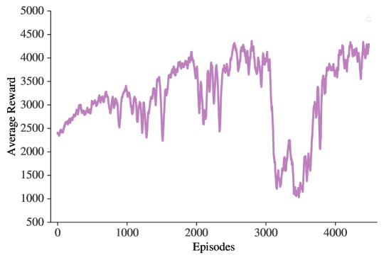
Figure 3: Training curve showing convergence of 20-period moving average reward for $\lambda=0.08$ and $\alpha=1$

Testing and Generalibility

We evaluate the performance of each trained model using test instances with varying values of $\lambda$ to assess their generalizability across different arrival patterns and optimization objectives. For this testing, we use 9 distinct values for $\lambda$, ranging from $0.01$ to $0.09$ in increments of $0.01$, and evaluate each of the 12 trained models against all of these values. Each model is tested against 1 in-sample scenario and 8 out-of-sample scenarios. Note that test scenarios with $\lambda\in\{0.01,0.03,0.05,0.07,0.09\}$ serve as out-of-sample scenarios for all trained models. As previously mentioned, each testing scenario consists of 10 simulation runs, with each run representing an 8-hour work shift.

Illustration of Real-time Order Picking

Figure 4 illustrates a pick cycle recommended by our trained DRL agent for a specific scenario with $\lambda=0.06$ and $\alpha=1$. In this context, the term ‘time’ refers to the elapsed time since the start of the work shift (not the computational time). Accordingly, the picker begins this cycle 661 seconds into the work shift with a full capacity of $K=20$. The blue square represents the depot, while the red square denotes the picker with its remaining capacity highlighted. Since the horizontal distance within aisles is negligible, orders within storage locations on both sides are shown as green dots inside the aisles. At 673 seconds, as depicted in Figure 4(a), the order picker arrives at aisle 9 and retrieves an item from the second row. Simultaneously, a new demand arises for an item on the third row in the same aisle. The picker efficiently fulfills all three pick requests in aisle 9 before moving sequentially to aisles 7 and 5, as indicated by the red line. Figure 4(b) illustrates the picker carrying five items with a remaining capacity of 15 units as it proceeds towards aisle 6 to pick up the next set of requested items. At this point, two new orders appear at position 13 in aisle 6. The DRL agent’s demand forecasting guided the picker to this aisle. Figure 4(c) shows the picker completing pick-ups in aisle 6 before returning to the depot via the same path. In Figure 4(d), the picker concludes the drop-offs at the depot, where each drop-off takes one second. This marks the end of the pick cycle, and the picker is prepared for the next assignment. Note that new orders have arrived at the warehouse at various time steps during the picker’s traversal. Throughout the pick cycle, the DRL agent dynamically prioritizes orders to minimize the average order fulfillment time.

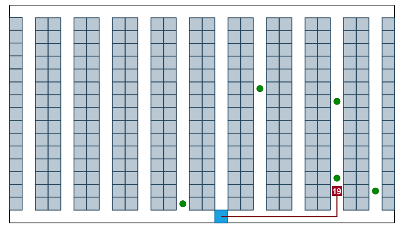
(a) Time (sec.): 673

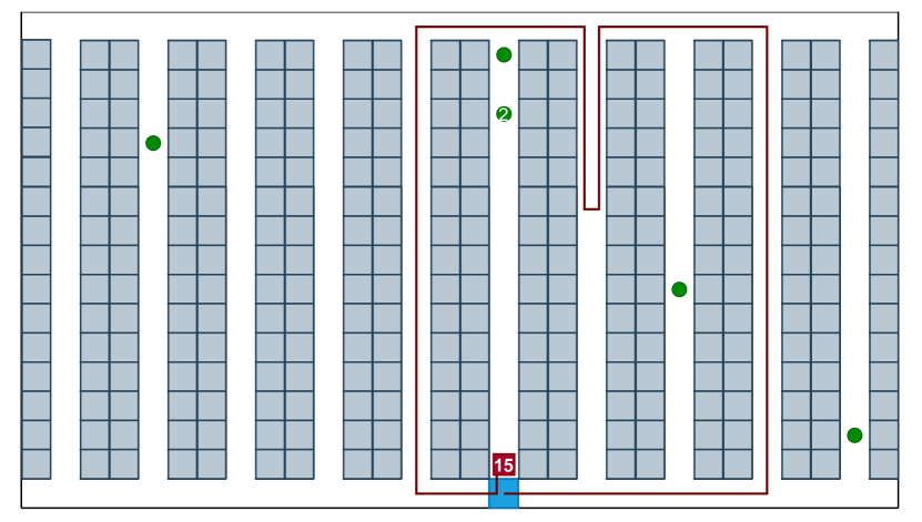
(b) Time (sec.): 735

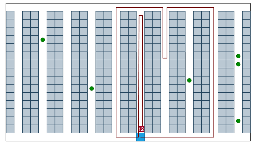
(c) Time (sec.): 766

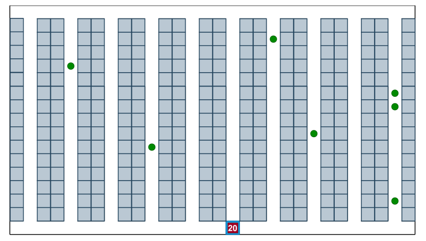
(d) Time (sec.): 775

Figure 4: Example demonstration of a pick cycle executed by the learned DRL agent with $\lambda=0.06$ and $\alpha=1$

5.3 Numerical Results

The results of our experiments are summarized in Tables 2, 3, and 4. Table 2 presents the average total distance traveled (ATDO) resulting from each model decisions for each instance type. The corresponding results for average order completion time (AOCT) and percentage of unfulfilled orders (PUO) are shown in Tables 3 and 4, respectively. Across these tables, the shaded cells highlight either the most desirable result or the most effective DRL model. Specifically, the trained model demonstrating the best average order completion time for each order arrival rate is highlighted. Next, we analyse the results and make a few observations.

The first observation is that, unsurprisingly, Baseline 1 results in the shortest distance traveled due to its strategy of waiting for the pick list to reach pick device capacity. This was expected, as by design, this approach allows the picker to follow the shortest possible path and move uninterrupted even when new customer orders arrive. However, as previously mentioned, the most crucial metric for optimizing warehouse operations is not the shortest distance traveled but the order completion times. Unfortunately, Baseline 1 has the worst performance in terms of average order completion times across all arrival rates and, consequently, the highest percentage of unfilled orders. Therefore, among the baselines, the variations of IRA—namely Baselines 2 through 4—are certainly better choices than Baseline 1.

Table 2: Performance comparison summary: Average Travel Distance per Order (ATDO)

DRL Model		ATDO (meters) w.r.t. $\lambda$
$\lambda$	$\alpha$	0.01	0.02	0.03	0.04	0.05	0.06	0.07	0.08	0.09
	0.1	37.73	55.83	86.42	111.15	109.81	95.24	80.81	65.61	48.50
	0.5	37.15	45.28	57.43	63.91	66.99	69.61	68.18	61.40	51.53
0.02	1.0	33.85	40.31	48.70	59.89	73.69	86.12	81.71	70.74	56.97
	0.1	61.93	79.65	87.51	88.83	84.83	77.18	69.63	63.03	55.31
	0.5	81.60	86.40	81.57	78.43	74.42	70.68	67.46	65.37	57.75
0.04	1.0	72.17	75.91	71.71	66.80	63.30	60.74	59.54	57.03	48.58
	0.1	65.78	106.23	106.92	88.80	75.32	61.26	53.19	46.19	52.29
	0.5	61.51	93.21	95.26	81.43	69.21	60.15	56.10	49.52	46.36
0.06	1.0	117.30	107.46	87.08	75.31	65.38	59.03	55.66	51.27	49.72
	0.1	71.71	145.70	198.54	177.00	143.14	103.99	75.88	57.51	47.08
	0.5	126.68	132.04	109.68	83.98	69.97	59.70	54.62	49.27	42.26
0.08	1.0	70.31	126.53	141.88	112.20	87.12	67.17	54.66	46.57	40.00
Baseline 1		8.18	8.14	8.20	8.18	8.14	8.09	8.19	8.17	8.19
Baseline 2		16.69	16.43	15.60	14.72	13.05	10.90	8.84	8.28	8.23
Baseline 3		16.78	16.59	15.71	14.68	13.01	10.88	8.84	8.28	8.23
Baseline 4		27.98	24.65	21.08	17.56	14.39	11.18	8.88	8.28	8.26
Baseline 5		27.74	24.37	20.86	17.45	14.35	11.15	8.88	8.28	8.26

Further analysis of baseline models also reveals that allowing pickers to re-route within cross-aisles enhances order completion times when order arrivals are frequent, i.e., $\lambda\geq 0.05$. However, the intervention routing strategy should be avoided within cross-aisles when order arrivals are less frequent ($\lambda<0.05$). This is evident when comparing Baselines 2 and 3, or Baselines 4 and 5, in Table 3. Notably, under scenarios with higher order arrival rates, all baseline models lead to a substantial number of unfulfilled orders within the work shift. For example, when $\lambda=0.9$, approximately 18% of orders remain unfulfilled. An exception occurs when $\lambda\leq 0.02$, where Baseline 4 surpasses our trained DRL models. In such cases of low arrival rates, a simple policy of shortest routing with intervention can be effective.

Table 3: Performance comparison summary: Average Order Completion Time (AOCT)

DRL Model		AOCT (seconds) w.r.t. $\lambda$
$\lambda$	$\alpha$	0.01	0.02	0.03	0.04	0.05	0.06	0.07	0.08	0.09
	0.1	89.9	122.0	182.9	268.4	307.6	368.4	461.3	550.2	764.5
	0.5	81.5	95.1	129.6	170.8	219.6	300.9	392.6	479.7	644.5
0.02	1.0	67.4	87.2	118.1	171.6	239.8	363.4	512.2	676.3	844.9
	0.1	150.5	160.9	178.8	208.3	238.2	278.2	340.8	460.5	740.1
	0.5	226.5	181.2	174.8	196.5	222.0	266.4	336.0	456.5	716.8
0.04	1.0	180.1	156.8	162.4	185.5	210.2	255.9	330.5	436.6	620.3
	0.1	136.0	192.6	218.8	227.3	236.3	262.3	305.1	402.0	809.6
	0.5	146.8	186.3	208.8	218.3	230.3	256.1	304.2	382.1	676.8
0.06	1.0	277.6	218.1	202.8	216.7	227.1	260.9	323.1	403.1	640.2
	0.1	175.1	332.8	460.3	427.0	400.5	378.9	378.3	403.7	513.1
	0.5	309.0	292.0	294.7	284.7	288.7	306.0	336.0	383.5	536.7
0.08	1.0	158.2	252.5	313.0	304.4	291.8	295.0	318.5	369.0	556.3
Baseline 1		1,217.1	751.6	593.0	512.1	471.7	445.1	560.0	1,526.2	2,809.3
Baseline 2		292.6	226.3	238.0	270.1	289.2	313.1	461.5	1,429.5	2,715.8
Baseline 3		294.5	229.0	242.9	270.2	286.8	311.6	460.2	1,425.6	2,710.1
Baseline 4		52.2	82.1	141.4	222.0	271.2	308.7	462.9	1,419.8	2,712.7
Baseline 5		54.6	87.1	148.3	225.2	271.0	308.8	461.2	1,418.4	2,711.8

Table 4: Performance comparison summary: Percentage of Unfulfilled Orders (PUO)

DRL Model		PUO (%) w.r.t. $\lambda$
$\lambda$	$\alpha$	0.01	0.02	0.03	0.04	0.05	0.06	0.07	0.08	0.09
	0.1	0.46	0.38	0.36	1.22	1.11	1.24	1.26	2.13	2.80
	0.5	0.40	0.27	0.45	0.54	0.66	0.91	1.21	1.82	2.16
0.02	1.0	0.64	0.36	0.30	0.60	0.85	1.20	1.72	2.72	2.99
	0.1	0.63	0.54	0.60	0.93	0.93	0.71	1.01	1.62	3.02
	0.5	1.23	0.67	0.50	0.75	0.69	0.72	1.00	1.77	2.78
0.04	1.0	0.63	0.67	0.60	0.74	0.56	0.79	0.92	1.69	2.19
	0.1	0.76	0.57	0.69	0.72	0.75	0.80	1.01	1.47	5.62
	0.5	0.84	0.65	0.62	0.93	0.74	0.71	0.95	1.40	3.47
0.06	1.0	0.80	0.93	0.57	0.73	0.69	0.69	1.01	1.54	2.66
	0.1	0.81	0.89	1.21	1.82	1.31	1.27	1.36	1.36	1.78
	0.5	1.87	0.86	1.12	1.11	0.86	0.95	1.17	1.27	1.89
0.08	1.0	0.66	0.77	1.08	1.25	0.96	1.03	0.97	1.25	2.27
Baseline 1		5.02	1.89	2.26	1.48	1.43	1.22	1.65	9.24	18.55
Baseline 2		0.92	0.57	0.58	1.02	0.71	0.89	1.15	9.06	18.30
Baseline 3		0.81	0.55	0.68	1.06	0.83	0.88	1.14	9.06	18.30
Baseline 4		0.07	0.25	0.32	0.94	0.69	1.17	1.18	8.86	18.30
Baseline 5		0.10	0.25	0.34	0.99	0.70	0.93	1.13	8.86	18.30

Comparing the baselines with our trained DRL models demonstrates that our DRL model significantly enhances both order throughput and fulfillment rates, even in scenarios not encountered during training. Based on the results from the trained DRL models, we recommend the following policies for training DRL models: Specifically, use training data that follows Poisson arrival rate parameters aligned with actual order arrival rates, as follows:

• Train with $\lambda=0.02$: For observed order arrival rates between 0.01 and 0.04

• Train with $\lambda=0.06$: For observed order arrival rates between 0.05 and 0.07

• Train with $\lambda=0.08$: For observed order arrival rates between 0.08 and 0.09

While the learned policies may lead to increased travel distances within the warehouses, they result in significant time savings overall. For example, in scenarios with $\lambda=0.09$, the recommended DRL model’s decision rules reduce AOCT by about 428% compared to baseline models. Moreover, our model drastically reduces the percentage of unfulfilled orders (PUO) to approximately 2%, compared to 18.3% for baselines during the 8-hour work shifts. Our results demonstrate that demand forecasting and order picking using reinforcement learning are highly effective strategies, particularly in scenarios with frequent order arrivals, i.e., $\lambda>0.02$.

Finally, our experiments demonstrate the remarkable robustness and transferability of our trained models across diverse testing scenarios with varying arrival rates. For each $\lambda$ used in training, we explored three values of $\alpha$, a parameter indirectly controlling the trade-off between prioritizing travel distance ($\alpha=0$) and order completion times ($\alpha=1$). While ‘$\alpha=1$’ performs well when training and testing data are closely aligned, we find that ‘$\alpha=0.5$’ provides superior robustness when real arrival rates may fluctuate slightly. Additionally, in test instances with higher arrival rates, all our trained models significantly outperformed benchmark algorithms in terms of AOCT and PUO. For example, in test instances with an arrival rate of $\lambda=0.08$, the worst-performing trained model still achieved an AOCT of 676.3 seconds, a significant improvement over the best baseline’s AOCT of 1418.4 seconds. These results underscore the real-world applicability of our proposed framework, as it maintains exceptional performance even under varying order arrival rates, making it well-suited for real-time deployment.

6 Conclusions

In this research, we propose a Deep Reinforcement Learning (DRL) model designed to solve the dynamic order picking problem within a single-block warehouse layout served by an autonomous picking device. Our results demonstrate that the model’s ability to forecast customer demands and adaptively learn efficient order picking policies leads to significant enhancements in overall warehouse operations. Furthermore, the additional experiments demonstrate the robustness of our proposed model through its strong performance on out-of-sample test instances with varying order arrival rates. This work provides a foundation for future research to explore more complex warehouse environments. In particular, the extension of this DRL framework to multi-block layouts and scenarios involving multiple coordinated picking devices presents promising avenues for further advancing the field of warehouse automation. By leveraging the forecasting and adapting capabilities of DRL, warehouse operations can be both efficient and responsive to the dynamic nature of customer demands.

References

- Beeks et al. (2022) Beeks, M., R. R. Afshar, Y. Zhang, R. Dijkman, C. Van Dorst, S. De Looijer. 2022. Deep reinforcement learning for a multi-objective online order batching problem. Proceedings of the International Conference on Automated Planning and Scheduling, vol. 32. 435–443.
- Begnardi et al. (2024) Begnardi, L., H. Baier, W. van Jaarsveld, Y. Zhang. 2024. Deep reinforcement learning for two-sided online bipartite matching in collaborative order picking. Asian Conference on Machine Learning. PMLR, 121–136.
- Cals et al. (2021) Cals, B., Y. Zhang, R. Dijkman, C. van Dorst. 2021. Solving the online batching problem using deep reinforcement learning. Computers & Industrial Engineering 156 107221.
- Çelk and Süral (2014) Çelk, M., H. Süral. 2014. Order picking under random and turnover-based storage policies in fishbone aisle warehouses. IIE Transactions 46(3) 283–300.
- Charkhgard and Savelsbergh (2015) Charkhgard, H., M. Savelsbergh. 2015. Efficient algorithms for travelling salesman problems arising in warehouse order picking. The ANZIAM Journal 57(2) 166–174.
- Dauod and Won (2022) Dauod, H., D. Won. 2022. Real-time order picking planning framework for warehouses and distribution centres. International Journal of Production Research 60(18) 5468–5487.
- De Koster et al. (2007) De Koster, R., T. Le-Duc, K. J. Roodbergen. 2007. Design and control of warehouse order picking: A literature review. European Journal of Operational Research 182(2) 481–501.
- Dunn et al. (2024) Dunn, G., H. Charkhgard, A. Eshragh, S. Mahmoudinazlou, E. Stojanovski. 2024. Deep reinforcement learning for picker routing problem in warehousing. arXiv preprint arXiv:2402.03525 .
- Giannikas et al. (2017) Giannikas, V., W. Lu, B. Robertson, D. McFarlane. 2017. An interventionist strategy for warehouse order picking: Evidence from two case studies. International Journal of Production Economics 189 63–76.
- Hall (1993) Hall, R. W. 1993. Distance approximations for routing manual pickers in a warehouse. IIE transactions 25(4) 76–87.
- Henn (2012) Henn, S. 2012. Algorithms for on-line order batching in an order picking warehouse. Computers & Operations Research 39(11) 2549–2563.
- Kaynov et al. (2024) Kaynov, I., M. van Knippenberg, V. Menkovski, A. van Breemen, W. van Jaarsveld. 2024. Deep reinforcement learning for one-warehouse multi-retailer inventory management. International Journal of Production Economics 267 109088.
- Li et al. (2019) Li, M. P., P. Sankaran, M. E. Kuhl, R. Ptucha, A. Ganguly, A. Kwasinski. 2019. Task selection by autonomous mobile robots in a warehouse using deep reinforcement learning. 2019 Winter Simulation Conference (WSC). IEEE, 680–689.
- Lu et al. (2016) Lu, W., D. McFarlane, V. Giannikas, Q. Zhang. 2016. An algorithm for dynamic order-picking in warehouse operations. European Journal of Operational Research 248(1) 107–122.
- Marchet et al. (2015) Marchet, G., M. Melacini, S. Perotti. 2015. Investigating order picking system adoption: a case-study-based approach. International Journal of Logistics Research and Applications 18(1) 82–98.
- Masae et al. (2020a) Masae, M., C. H. Glock, E. H. Grosse. 2020a. Order picker routing in warehouses: A systematic literature review. International Journal of Production Economics 224 107564.
- Masae et al. (2020b) Masae, M., C. H. Glock, P. Vichitkunakorn. 2020b. Optimal order picker routing in the chevron warehouse. IISE Transactions 52(6) 665–687.
- Muter and Öncan (2022) Muter, İ., T. Öncan. 2022. Order batching and picker scheduling in warehouse order picking. IISE Transactions 54(5) 435–447.
- Pansart et al. (2018) Pansart, L., N. Catusse, H. Cambazard. 2018. Exact algorithms for the order picking problem. Computers & Operations Research 100 117–127.
- Rasmi et al. (2022) Rasmi, S. A. B., Y. Wang, H. Charkhgard. 2022. Wave order picking under the mixed-shelves storage strategy: A solution method and advantages. Computers & Operations Research 137 105556.
- Ratliff and Rosenthal (1983) Ratliff, H. D., A. S. Rosenthal. 1983. Order-picking in a rectangular warehouse: a solvable case of the traveling salesman problem. Operations Research 31(3) 507–521.
- Roodbergen and De Koster (2001) Roodbergen, K. J., R. De Koster. 2001. Routing order pickers in a warehouse with a middle aisle. European Journal of Operational Research 133(1) 32–43.
- Roy et al. (2019) Roy, D., S. Nigam, R. de Koster, I. Adan, J. Resing. 2019. Robot-storage zone assignment strategies in mobile fulfillment systems. Transportation Research Part E: Logistics and Transportation Review 122 119–142.
- Scholz et al. (2016) Scholz, A., S. Henn, M. Stuhlmann, G. Wäscher. 2016. A new mathematical programming formulation for the single-picker routing problem. European Journal of Operational Research 253(1) 68–84.
- Scholz and Wäscher (2017) Scholz, A., G. Wäscher. 2017. Order batching and picker routing in manual order picking systems: the benefits of integrated routing. Central European Journal of Operations Research 25(2) 491–520.
- Silva et al. (2020) Silva, A., L. C. Coelho, M. Darvish, J. Renaud. 2020. Integrating storage location and order picking problems in warehouse planning. Transportation Research Part E: Logistics and Transportation Review 140 102003.
- Sobhanan et al. (2023) Sobhanan, A., J. Park, J. Park, C. Kwon. 2023. Genetic algorithms with neural cost predictor for solving hierarchical vehicle routing problems. arXiv preprint arXiv:2310.14157 .
- Tian et al. (2024) Tian, R., M. Lu, H. Wang, B. Wang, Q. Tang. 2024. Iacppo: A deep reinforcement learning-based model for warehouse inventory replenishment. Computers & Industrial Engineering 187 109829.
- Tsotsos et al. (2019) Tsotsos, J., I. Kotseruba, A. Andreopoulos, Y. Wu. 2019. Why does data-driven beat theory-driven computer vision? Proceedings of the IEEE/CVF International Conference on Computer Vision Workshops. 2057–2060.
- Van Gils et al. (2018) Van Gils, T., K. Ramaekers, A. Caris, R. B. De Koster. 2018. Designing efficient order picking systems by combining planning problems: State-of-the-art classification and review. European journal of operational research 267(1) 1–15.
- Winkelhaus et al. (2021) Winkelhaus, S., E. H. Grosse, S. Morana. 2021. Towards a conceptualisation of order picking 4.0. Computers & Industrial Engineering 159 107511.
- Yang et al. (2021) Yang, P., Z. Zhao, Z.-J. M. Shen. 2021. A flow picking system for order fulfillment in e-commerce warehouses. IISE Transactions 53(5) 541–551.