Structure-preserving approximations of the Serre-Green-Naghdi
equations in standard and hyperbolic form

Abstract

We develop structure-preserving numerical methods for the Serre-Green-Naghdi equations, a model for weakly dispersive free-surface waves. We consider both the classical form, requiring the inversion of a non-linear elliptic operator, and a hyperbolic approximation of the equations, allowing fully explicit time stepping. Systems for both flat and variable topography are studied. Our novel numerical methods conserve both the total water mass and the total energy. In addition, the methods for the original Serre-Green-Naghdi equations conserve the total momentum for flat bathymetry. For variable topography, all the methods proposed are well-balanced for the lake-at-rest state. We provide a theoretical setting allowing us to construct schemes of any kind (finite difference, finite element, discontinuous Galerkin, spectral, etc.) as long as summation-by-parts operators are available in the chosen setting. Energy-stable variants are proposed by adding a consistent high-order artificial viscosity term. The proposed methods are validated through a large set of benchmarks to verify all the theoretical properties. Whenever possible, comparisons with exact, reference numerical, or experimental data are carried out. The impressive advantage of structure preservation, and in particular energy preservation, to resolve accurately dispersive wave propagation on very coarse meshes is demonstrated by several of the tests.

1 Introduction

This paper is devoted to the structure-preserving numerical approximation of the fully nonlinear, weakly dispersive Serre-Green-Naghdi (SGN) equations for free-surface hydrodynamics. Dispersive free-surface waves occur in a wide variety of phenomena going from the propagation of tsunamis [52, 73, 3], to estuarine dynamics and wave propagation in natural as well man made environments [128, 9, 17, 39, 60]. Many of these applications involve multi-scale wave physics, with often large domains and long-time/distance propagation. Depth averaged Boussinesq-type equations are used in many existing operational codes for hazard assessment (see e.g. [68, 64] and references therein). These models can be written as a perturbation of the hyperbolic shallow water equations with a dispersive term, which accounts for some of the vertical kinematic lost in the depth averaging [71]. Among these models, the SGN system [119, 53, 131] accounts for the full nonlinearity of the wave propagation and transformation, and is endowed with a rigorous estimate of the energy associated to the wave dynamics (see e.g. [37, 50, 71, 63]) which can be used as a rigorous criterion to estimate the dissipation during the propagation process. In the literature, two main writings of the SGN equations have been used for the purpose of numerical approximation: a classical one involving the inversion of a nonlinear elliptic operator to evaluate the time variation of the velocity [71, 63, 50], and a system based on a hyperbolic relaxation of the dispersion operator [37, 34]. Both forms are considered here.

Realistic operational applications require being able to run multi-scale simulations on reasonably coarse meshes to obtain fast predictions. A lot of focus is being put on deploying operational codes on modern high-performance parallel architectures [134, 125, 20]. In this work, we consider the other end of the process, and propose improved numerical methods. In the literature we find many different numerical approaches to approximate Boussinesq-type, dispersive shallow water equations. Many such techniques involve some high-order approximation in space and time, with possibly ad-hoc treatments for the dispersive terms (hyperbolization, or some lower-order approximation) to combine efficiency and good numerical dispersion [131, 35, 62, 116, 94, 72, 83, 41, 29, 74, 13, 15, 127, 63]. Some authors also propose methods with some strong energy stability/dissipation property [122, 95], by imitation of what is usually done for hyperbolic conservation laws with entropy stability. Few recent works focus on approximations guaranteeing exact energy conservation [108, 84, 70] at the discrete level.

The theoretical and numerical results discussed in [33, 31, 12, 8] show that there is a very delicate interaction between dissipation, dispersion, and non-linearity. In particular, while in the purely dispersive setting many initial conditions lead to appearance of solitary wave fission, in presence of finite dissipation one obtains travelling waves with finite stationary wavelength and much lower amplitudes. In this respect, while recent work has shown that discontinuous solutions for Boussinesq models can be constructed [49, 30, 58], such constructions do not rely, as in the case of hyperbolic balance laws, on the notion of a dissipative solution. Admissibility conditions for these problems are formulated based on geometrical considerations in phase space, and relate to the celerities of the solution fronts. There is no notion on the sign of the energy evolution in such conditions. It is thus unclear whether one should use numerical dissipation when solving non-dissipative dispersive equations as a means of stabilization. This is a major difference between dispersive models and hyperbolic ones. In addition, the recent work by Jouy et al. [60] has shown that numerical dissipation plays in practice the exact same role of a physical dissipative regularization. In particular, when using high-order schemes embedding dissipation a gross underestimation of the wave amplitudes may be obtained on coarse meshes. This is not the case for non-dissipative methods. The results of [60] show that this issue occurs not only for non-dissipative models, but also in presence of physical dissipation terms in the model, e.g., due to friction terms. Our objective is thus to investigate the construction and validation of structure-preserving methods for the SGN equations, namely methods which conserve within machine accuracy as many physical properties as possible, including energy, and which is well-balanced with respect to the well-known lake-at-rest state.

To this end we use the framework of summation-by-parts (SBP) operators and split forms [43] as a systematic approach to build exactly energy-conservative semidiscretizations. The idea is to follow step-by-step the continuous derivation of the energy balance, and combine the use of SBP differentiation operators, which allow to mimic integration by parts, and use appropriate split forms of the differential equations to mimic the product and chain rule. To obtain a fully conservative method, the resulting ordinary differential equations in time can be integrated using relaxation Runge-Kutta (RRK) schemes, which are a small modification of classical Runge-Kutta methods allowing to preserve appropriate invariants [66, 113].

The paper is organized as follows. In the following Section 2, we briefly review the techniques that we use for spatial and temporal discretizations. In particular, we describe how split forms of the equations can be used to derive energy-conserving discretizations using SBP operators. Next, we review such energy-conserving split forms of the classical shallow water equations in Section 3. In Section 4, we review the classical SGN equations in flat bathymetry as well as their hyperbolic approximation. To prepare the remainder of this article, we also explain how to pass from the hyperbolic approximation to the original system. Next, we derive a structure-preserving split form and discretization of the hyperbolic approximation with flat bathymetry in Section 5. We begin with the hyperbolic approximation since there are less complicated higher-derivative terms in this case, making it easier to derive an energy-conserving split form. Using the previously established translation rules, we use these results to derive corresponding structure-preserving methods for the original SGN equations in Section 6. We extend the investigations to the case of variable bathymetry first for the hyperbolic approximation in Section 7 and to the classical SGN equations in Sections 8 and 9. We describe how to add stabilizing artificial viscosity/dissipation in Section 10. Afterwards, we validate our implementation and present numerical experiments in Section 11. Finally, we summarize our results and give an outlook on future work in Section 12.

2 Brief review of split forms and discretization techniques

In this section, we briefly review the techniques that we use for spatial and temporal discretizations. In general, we will use the method of lines, starting with a semidiscretization in space followed by a time integration.

2.1 Split forms

Consider Burgers’ equation

$$u_{t}+\left(\frac{1}{2}u^{2}\right)_{x}=0$$ (1)

with periodic boundary conditions. As is well known, a smooth solution satisfies the energy equality

$$\left(\frac{1}{2}u^{2}\right)_{t}+\left(\frac{1}{3}u^{3}\right)_{x}=0.$$ (2)

Thus, the total energy (squared $\displaystyle L^{2}$ norm) is conserved. To prove this, one would typically multiply the PDE by $\displaystyle u$ and use the chain rule. However, discrete derivative operators can in general not satisfy a discrete version of the chain rule, in particular for higher-order operators [100]. Thus, we will use the split form [117, eq. (6.40)]

$$u_{t}+\frac{1}{3}(u^{2})_{x}+\frac{1}{3}uu_{x}=0.$$ (3)

Indeed, multiplying Burgers’ equation by the solution $\displaystyle u$ and integrating over the domain yields

$$\frac{1}{2}\frac{\operatorname{d\!}}{\operatorname{d\!}t}\int u^{2}\operatorname{d\!}x=\int uu_{t}\operatorname{d\!}x=-\frac{1}{3}\int u(u^{2})_{x}\operatorname{d\!}x-\frac{1}{3}\int u^{2}u_{x}\operatorname{d\!}x=0.$$ (4)

Hence, energy conservation can be shown using only integration by parts. To obtain a semidiscretization satisfying the energy conservation law at the discrete level, we just need to use the split form derived at the continuous level and apply discrete derivative operators satisfying a discrete equivalent of integration by parts.

Although the split form looks like it results in a non-conservative discretization, one can show that the total mass is still conserved since

$$\frac{\operatorname{d\!}}{\operatorname{d\!}t}\int u\operatorname{d\!}x=-\frac{1}{3}\int(u^{2})_{x}\operatorname{d\!}x-\frac{1}{3}\int u_{x}u\operatorname{d\!}x=0,$$ (5)

using again only integration by parts. Moreover, it can be shown that the discretization of the split form is even locally conservative when discretized with SBP operators [43]. This also holds for more general flux differencing discretizations that can be entropy-stable but do not need to be related to a split form [42].

2.2 Summation-by-parts operators

SBP operators are discrete derivative operators designed to mimic integration by parts at the discrete level. Originally, SBP operators were introduced for finite difference methods [69, 120], but they can also be used for finite volume [88, 89], continuous finite element [57, 56, 1], discontinuous Galerkin [47, 14, 16], and flux reconstruction methods [59, 110]. A good overview can be obtained from the review articles [123, 38] and the application of various methods from the SBP framework to dispersive wave equations in [108].

We consider periodic boundary conditions in this article. Thus, we will only briefly recap the corresponding properties of periodic SBP operators. Further discussions and examples can be found in [123, 38, 108]. We use a nodal collocation approach and discretize the spatial domain using point values of the unknowns at given grid points $\displaystyle x_{i}$. The discretized version of a function $\displaystyle u$ is denoted by $\displaystyle\boldsymbol{u}$ with $\displaystyle\boldsymbol{u}_{i}=u(x_{i})$. In particular, $\displaystyle\boldsymbol{1}=(1,\dots,1)^{T}$. Nonlinear operations are performed pointwise, e.g., $\displaystyle(\boldsymbol{u}^{2})_{i}=\boldsymbol{u}_{i}^{2}$.

Definition 1.

A periodic SBP operator on the domain $\displaystyle[x_{\mathrm{min}},x_{\mathrm{max}}]$ consists of a grid $\displaystyle\boldsymbol{x}$, a symmetric and positive definite mass/norm matrix $\displaystyle M$ satisfying $\displaystyle\boldsymbol{1}^{T}M\boldsymbol{1}=x_{\mathrm{max}}-x_{\mathrm{min}}$, and a consistent derivative operator $\displaystyle D$ such that

$$MD+D^{T}M=0.$$ (6)

It is called diagonal-norm operator if $\displaystyle M$ is diagonal.

A consistent derivative operator $\displaystyle D$ differentiaties constants exactly, i.e., $\displaystyle D\boldsymbol{1}=\boldsymbol{0}$. A classical example of a periodic SBP operator is given by central second-order finite differences, where mass matrix is the identity matrix scaled by the grid spacing $\displaystyle\Delta x$ and the stencil coefficients of the derivative operator are $\displaystyle\Delta x^{-1}(-1/2,0,1/2)$.

The definition above introduces first-derivative SBP operators. Since we also need higher derivatives for the dispersive terms, we will use second-derivative SBP operators [82, 80] as well. Since the second-derivative terms of the Serre-Green-Naghdi equations have variable coefficients, we will use upwind operators to construct them in a general way [81]. See also [108, 92] for discussions of upwind SBP operators and discontinuous Galerkin methods for second-derivative terms.

Definition 2.

A periodic upwind SBP operator on the domain $\displaystyle[x_{\mathrm{min}},x_{\mathrm{max}}]$ consists of a grid $\displaystyle\boldsymbol{x}$, a symmetric and positive definite mass/norm matrix $\displaystyle M$ satisfying $\displaystyle\boldsymbol{1}^{T}M\boldsymbol{1}=x_{\mathrm{max}}-x_{\mathrm{min}}$, and two consistent derivative operators $\displaystyle D_{\pm}$ such that

$$MD_{+}+D_{-}^{T}M=0,\qquad M(D_{+}-D_{-})\text{ is negative semidefinite}.$$ (7)

It is called diagonal-norm operator if $\displaystyle M$ is diagonal.

We will frequently use that the average $\displaystyle D=(D_{+}+D_{-})/2$ of upwind SBP operators is a central SBP operator [81]. A classical example of periodic upwind SBP operators is given by the one-sided first-order finite differences, where the mass matrix is again the identity matrix scaled by the grid spacing $\displaystyle\Delta x$ and the stencil coefficients of the upwind derivative operator are $\displaystyle\Delta x^{-1}(-1,1,0)$ and $\displaystyle\Delta x^{-1}(0,-1,1)$. Thus, the corresponding central SBP operator is given by the coefficients $\displaystyle\Delta x^{-1}(-1/2,0,1/2)$.

To get a second-derivative operator, one can apply a first-derivative operator twice. For the classical second-order central SBP operator, this results in the wide-stencil operator with coefficients $\displaystyle\Delta x^{-2}(1/4,0,-1/2,0,1/4)$. A better approximation is usually given by the combination of upwind operators, e.g., $\displaystyle D_{+}D_{-}$ with stencil coefficients $\displaystyle\Delta x^{-2}(1,-2,1)$.

In this article, we will only use diagonal-normal SBP operators. We will use the quadrature rule induced by the mass matrix to compute discrete versions of integrals or the discrete $\displaystyle L^{2}$ error.

2.3 Time integration methods using relaxation

We will use explicit Runge-Kutta methods for time integration. Since such explicit time integration methods cannot guarantee conservation (or dissipation) of nonlinear invariants such as the energy [101, 90, 105, 61, 76, 109, 121], we will use relaxation to enforce the conservation of the energy [66, 114, 107]. This approach has its origins in an idea of Sanz-Serna [118]. It has been applied successfully to compressible flows [133, 103, 130] and various other systems conserving or dissipating an energy/entropy functional. It is particularly useful for long-time simulations of dispersive wave equations and Hamiltonian systems [108, 106, 84, 111, 7, 135].

The basic idea is as follows. Consider an ODE $\displaystyle u^{\prime}=f(u)$ and assume that the ODE conserves an energy $\displaystyle\eta(u)$, i.e., $\displaystyle\forall u\colon\eta^{\prime}(u)f(u)=0$. Given a one-step method computing $\displaystyle u^{n+1}\approx u(t^{n+1})$ from $\displaystyle u^{n}\approx u(t^{n})$, we enforce conservation of the energy $\displaystyle\eta$ by projecting the numerical solution along the secant line connecting $\displaystyle u^{n}$ and $\displaystyle u^{n+1}$ onto the level set $\displaystyle\eta(u)=\eta(u^{n})$. Thus, we need to solve the scalar root finding problem

$$\eta(u^{n+1}_{\gamma})=\eta(u^{n}),\quad u^{n+1}_{\gamma}=u^{n}+\gamma(u^{n+1}-u^{n}),$$ (8)

for the relaxation parameter $\displaystyle\gamma$. The general theory of relaxation methods shows that there is a unique solution $\displaystyle\gamma=1+\mathcal{O}(\Delta t^{p-1})$ under rather general assumptions [107], where $\displaystyle p$ is the order of accuracy of the time integration method. Continuing the numerical integration with $\displaystyle u^{n+1}_{\gamma}$ instead of $\displaystyle u^{n+1}$ guarantees conservation of the energy $\displaystyle\eta$, of all linear invariants, and at least the same order of accuracy $\displaystyle p$ as the original method if the relaxed solution is interpreted as $\displaystyle u^{n+1}_{\gamma}\approx u(t^{n+1}_{\gamma})$, where the relaxed time is $\displaystyle t^{n+1}_{\gamma}=t^{n}+\gamma\Delta t$.

3 Split forms of the classical shallow water equations

The Serre-Green-Naghdi equations [119, 53, 131] (see also [71] and references therein) and their hyperbolic approximation [37, 13] are extensions of the classical shallow water equations by additional terms modeling dispersive effects. To prepare deriving structure-preserving discretizations, we first consider some split forms of the classical shallow water (Saint-Venant) equations.

3.1 Flat bathymetry

Consider the classical shallow water equations with constant bathymetry

$$h_{t}+(hu)_{x}=0,$$ (9)

$$(hu)_{t}+\left(hu^{2}+\frac{1}{2}gh^{2}\right)_{x}=0,$$

where $\displaystyle h$ denotes the water height, $\displaystyle u$ the velocity, and $\displaystyle g$ the gravitational constant. The system admits the energy conservation law [10, 44]

$$\biggl{(}\underbrace{\frac{1}{2}gh^{2}+\frac{1}{2}hu^{2}}_{=E}\biggr{)}_{t}+\biggl{(}\underbrace{gh^{2}u+\frac{1}{2}hu^{3}}_{=F}\biggr{)}_{x}=0.$$ (10)

A split form of the equations can be used to prove energy conservation using only integration by parts, e.g., [48, 132]. Indeed, there is even a two-parameter family of energy-conserving split forms of the classical shallow water equations [99]. A simplified version discarding some higher-order terms of [99, Section 4.2] reads

$$h_{t}+\alpha(hu)_{x}+(1-\alpha)h_{x}u+(1-\alpha)hu_{x}=0,$$ (11)

$$(hu)_{t}+(1-\alpha)g(h^{2})_{x}-(1-2\alpha)ghh_{x}$$

$$\qquad+\frac{\alpha}{2}(hu^{2})_{x}+\frac{1-\alpha}{2}h(u^{2})_{x}+\frac{1-\alpha}{2}h_{x}u^{2}+\frac{1}{2}(hu)_{x}u+\frac{1}{2}huu_{x}=0.$$

To simplify the following derivation, we focus on the split form (11) with $\displaystyle\alpha=0$, i.e.,

$$h_{t}+h_{x}u+hu_{x}=0,$$ (12)

$$(hu)_{t}+g(h^{2})_{x}-ghh_{x}+\frac{1}{2}h(u^{2})_{x}+\frac{1}{2}h_{x}u^{2}+\frac{1}{2}(hu)_{x}u+\frac{1}{2}huu_{x}=0.$$

Furthermore, to simplify the treatment of the elliptic terms in the Serre-Green-Naghdi equations, we will use primitive variables $\displaystyle(h,u)$ instead of the conservative variables $\displaystyle(h,hu)$ in the following. Thus, using the product rule in time

$$(hu)_{t}=hu_{t}+h_{t}u=hu_{t}-h_{x}u^{2}-huu_{x},$$ (13)

the split form (12) becomes

$$h_{t}+h_{x}u+hu_{x}=0,$$ (14)

$$hu_{t}+g(h^{2})_{x}-ghh_{x}+\frac{1}{2}h(u^{2})_{x}-\frac{1}{2}h_{x}u^{2}+\frac{1}{2}(hu)_{x}u-\frac{1}{2}huu_{x}=0.$$

To prepare the following arguments, we will demonstrate how to obtain conservation of total water mass, momentum, and energy.

3.1.1 Flat bathymetry: conservation of the total water mass

The spatial terms of the first equation of (14) cancel when integrated over the periodic domain due to integration by parts, i.e.,

$$0=\int h_{t}\operatorname{d\!}x+\int h_{x}u\operatorname{d\!}x+\int hu_{x}\operatorname{d\!}x=\frac{\operatorname{d\!}}{\operatorname{d\!}t}\int h\operatorname{d\!}x.$$ (15)

Note that the two terms vanishing via integration by parts yield exactly the difference of the flux $\displaystyle hu$ at the periodic boundaries.

3.1.2 Flat bathymetry: conservation of the total momentum

The time derivative of the momentum is

$$(hu)_{t}=h_{t}u+hu_{t}.$$ (16)

Thus, we multiply the first equation of (14) by $\displaystyle u$, add it to the second equation, integrate over the periodic domain, and obtain

$$0 =\int(hu)_{t}\operatorname{d\!}x+\int h_{x}u^{2}\operatorname{d\!}x+\int huu_{x}\operatorname{d\!}x+\int g(h^{2})_{x}\operatorname{d\!}x-\int ghh_{x}\operatorname{d\!}x$$ (17)

$$\quad+\frac{1}{2}\int h(u^{2})_{x}\operatorname{d\!}x-\frac{1}{2}\int h_{x}u^{2}\operatorname{d\!}x+\frac{1}{2}\int(hu)_{x}u\operatorname{d\!}x-\frac{1}{2}\int huu_{x}\operatorname{d\!}x$$

$$=\int(hu)_{t}\operatorname{d\!}x+\int g(h^{2})_{x}\operatorname{d\!}x-\int ghh_{x}\operatorname{d\!}x$$

$$\quad+\frac{1}{2}\int h(u^{2})_{x}\operatorname{d\!}x+\frac{1}{2}\int h_{x}u^{2}\operatorname{d\!}x+\frac{1}{2}\int(hu)_{x}u\operatorname{d\!}x+\frac{1}{2}\int huu_{x}\operatorname{d\!}x.$$

Using integration by parts, the two $\displaystyle gh^{2}$ terms yield a boundary term $\displaystyle gh^{2}/2$. The first two terms of the last line as well as the last two terms cancel due to integration by parts, respectively, resulting in the boundary terms $\displaystyle hu^{2}/2$ and $\displaystyle hu^{2}/2$. Thus, all terms canceling via integration by parts sum up to the expected flux $\displaystyle gh^{2}/2+hu^{2}$. This shows that for exact time integration momentum is conserved.

3.1.3 Flat bathymetry: conservation of the total energy

The time derivative of the energy $\displaystyle E$ (10) is

$$E_{t}=\left(\frac{1}{2}gh^{2}+\frac{1}{2}hu^{2}\right)_{t}=ghh_{t}+huu_{t}.$$ (18)

Thus, we multiply the first equation of (14) by $\displaystyle gh$, the second equation by $\displaystyle u$, add them, and obtain

$$0 =E_{t}+ghh_{x}u+gh^{2}u_{x}+g(h^{2})_{x}u-ghh_{x}u+\frac{1}{2}hu(u^{2})_{x}-\frac{1}{2}h_{x}u^{3}+\frac{1}{2}(hu)_{x}u^{2}-\frac{1}{2}hu^{2}u_{x}$$ (19)

$$=E_{t}+g\left(h^{2}u_{x}+(h^{2})_{x}u\right)+\frac{1}{2}\left(hu(u^{2})_{x}+(hu)_{x}u^{2}\right)-\frac{1}{2}\left(h_{x}u^{3}+hu^{2}u_{x}\right).$$

We see that all pairs of terms in parentheses cancel when integrating over the periodic domain due to integration by parts, resulting in the expected flux terms $\displaystyle F=gh^{2}u+hu^{3}/2$. Thus, the total energy is conserved, if the time integration is exact.

3.2 Variable bathymetry

The classical shallow water equations with variable bathymetry are

$$h_{t}+(hu)_{x}=0,$$ (20)

$$(hu)_{t}+\left(hu^{2}+\frac{1}{2}gh^{2}\right)_{x}+ghb_{x}=0,$$

where $\displaystyle b$ denotes the bathymetry (bottom topography). The system admits the energy conservation law [10, 44, 48]

$$\biggl{(}\underbrace{\frac{1}{2}gh^{2}+ghb+\frac{1}{2}hu^{2}}_{=E}\biggr{)}_{t}+\biggl{(}\underbrace{gh^{2}u+ghbu+\frac{1}{2}hu^{3}}_{=F}\biggr{)}_{x}=0.$$ (21)

The generalization to variable bathymetry of the split form (14) of [99, Section 5.3] is

$$h_{t}+h_{x}u+hu_{x}=0,$$ (22)

$$hu_{t}+g\bigl{(}h(h+b)\bigr{)}_{x}-g(h+b)h_{x}+\frac{1}{2}h(u^{2})_{x}-\frac{1}{2}h_{x}u^{2}+\frac{1}{2}(hu)_{x}u-\frac{1}{2}huu_{x}=0.$$

Conservation of the total water mass follows as in the case of flat bathymetry. Since (22) is the same as the previous split form (14) for flat bathymetry $\displaystyle b=0$, conservation of the total momentum follows for constant bottom topography as well. In the energy rate of change $\displaystyle E_{t}$, we get the new term $\displaystyle gbh_{t}$, leading to the additional terms

$$gh_{x}bu+ghbu_{x}+g(hb)_{x}u-gh_{x}bu=g\left(hbu_{x}+(hb)_{x}u\right),$$ (23)

which vanish due to integration by parts when integrating over the periodic domain. Thus, the total energy is conserved for variable bathymetry as well.

Moreover, the split form (22) is well-balanced, i.e., it preserves the lake-at-rest steady state $\displaystyle h+b=\mathrm{const}$, $\displaystyle u=0$. Indeed, the time derivative of $\displaystyle h$ vanishes for $\displaystyle u=0$, and the time derivative of the velocity is given by

$$0=hu_{t}+g\bigl{(}h(h+b)\bigr{)}_{x}-g(h+b)h_{x}=hu_{t}g(h+b)h_{x}-g(h+b)h_{x}=hu_{t}$$ (24)

if $\displaystyle h+b=\mathrm{const}$ additionally. All of these properties still hold for semidiscretizations using periodic SBP operators.

4 Review of the Serre-Green-Naghdi equations for flat bathymetry

In this section, we review the classical form of the Serre-Green-Naghdi equations for flat bathymetry as well as their hyperbolic approximation. We present the associated energy conservation laws and describe how to pass from one set of equations to the other to prepare the derivations later in this paper.

4.1 Equations in classical form and elliptic operator

On a flat bathymetry, the SGN equations can be written as

$$h_{t}+(hu)_{x}=0,$$ (25)

$$(hu)_{t}+\left(hu^{2}+\frac{1}{2}gh^{2}+\tilde{p}\right)_{x}=0,$$

$$\tilde{p}=-\dfrac{1}{3}\left(h^{3}(\dot{u})_{x}-2h^{3}u_{x}^{2}\right),$$

with the classical notation for the material derivative $\displaystyle\dot{a}=a_{t}+ua_{x}$. As in Section 3, $\displaystyle h$ is the water height, $\displaystyle u$ the velocity, and $\displaystyle g$ the gravitational constant. Compared to the shallow water equations (9), the SGN equations (25) contain an additional non-hydrostatic pressure $\displaystyle\tilde{p}$. This system is known to admit an energy conservation law reading

$$\biggl{(}\underbrace{\frac{1}{2}gh^{2}+\frac{1}{2}hu^{2}+\frac{1}{6}h(\dot{h})^{2}}_{=E}\biggr{)}_{t}+\biggl{(}\underbrace{gh^{2}u+\frac{1}{2}hu^{3}+\frac{1}{6}h(\dot{h})^{2}u+\tilde{p}u}_{=F}\biggr{)}_{x}=0.$$ (26)

Note that both the energy $\displaystyle E$ and the energy flux $\displaystyle F$ are extensions of the corresponding quantities for the shallow water equations (10). Our objective is to construct discrete approximations of the SGN system preserving exactly the energy conservation law (26).

Note that to advance in time system (25) requires the inversion of the operator $\displaystyle\mathcal{T}(u_{t})$, where

$$\mathcal{T}(v)=hv-\dfrac{1}{3}(h^{3}v_{x})_{x}.$$ (27)

Indeed, writing system (25) in primitive variables we have

$$h_{t}+(hu)_{x}=0,$$ (28)

$$hu_{t}-\frac{1}{3}(h^{3}u_{tx})_{x}+\frac{1}{2}g(h^{2})_{x}+huu_{x}+p_{x}=0,$$

$$p=\frac{1}{3}h^{3}u_{x}^{2}-\frac{1}{3}h^{3}uu_{xx},$$

where we have rewritten the non-hydrostatic pressure as

$$\tilde{p}=-\frac{1}{3}(h^{3}u_{tx})_{x}+p,$$ (29)

and calculated

$$\tilde{p} =-\frac{1}{3}\left(h^{3}(\dot{u})_{x}-2h^{3}u_{x}^{2}\right)=-\frac{1}{3}\left(h^{3}(u_{t}+uu_{x})_{x}-2h^{3}u_{x}^{2}\right)$$ (30)

$$=-\frac{1}{3}h^{3}u_{tx}-\frac{1}{3}h^{3}uu_{xx}+\frac{1}{3}h^{3}u_{x}^{2}.$$

This shows the appearance of the elliptic operator $\displaystyle\mathcal{T}(u_{t})$ (27) whose inversion is required to obtain $\displaystyle u_{t}$.

4.2 1-D augmented Lagrangian hyperbolic system

In this work we will also study the structure-preserving approximation of the hyperbolic augmented Lagrangian formulation of the fully-nonlinear SGN equations reading [37, 126]

$$h_{t}+(hu)_{x}=0,$$ (31)

$$(hu)_{t}+\bigg{(}hu^{2}+\frac{1}{2}gh^{2}+\frac{\lambda}{3}\eta(1-\eta/h)\bigg{)}_{x}=0,$$

$$(hw)_{t}+(hwu)_{x}=\lambda(1-\eta/h),$$

$$(h\eta)_{t}+(h\eta u)_{x}=hw.$$

For $\displaystyle\lambda=0$, we recover the usual hyperbolic shallow water system (9) from the first two equations. In compact form, we can write the above system as (with obvious definitions)

$$\mathbf{U}_{t}+\mathbf{F}_{x}=\mathbf{S}.$$

This system is hyperbolic, with characteristic speeds $\displaystyle\lambda_{1/4}=u\mp c$ and $\displaystyle\lambda_{2/3}=u$, where the celerity is given by

$$c^{2}=gh+\lambda\dfrac{\eta^{2}}{h^{2}}.$$

The model can be shown to admit the mathematical entropy (energy) conservation law

$$\biggl{(}\underbrace{\frac{1}{2}gh^{2}+\frac{1}{2}hu^{2}+\frac{1}{6}hw^{2}+\frac{\lambda}{6}h(1-\eta/h)^{2}}_{=E}\biggr{)}_{t}+\biggl{(}\underbrace{gh^{2}u+\frac{1}{2}hu^{3}+\frac{1}{6}hw^{2}u+\frac{\lambda}{6}h(1-\eta^{2}/h^{2})u}_{=F}\biggr{)}_{x}=0.$$ (32)

Please note again that the energy $\displaystyle E$ and the energy flux $\displaystyle F$ are extensions of the corresponding quantities for the shallow water equations (10). In primitive variables, the system (31) reads

$$h_{t}+(hu)_{x}=0,$$ (33)

$$hu_{t}+\frac{1}{2}g(h^{2})_{x}+huu_{x}+\left(\frac{\lambda}{3}\eta(1-\eta/h)\right)_{x}=0,$$

$$hw_{t}+huw_{x}=\lambda(1-\eta/h),$$

$$\eta_{t}+\eta_{x}u=w.$$

4.3 Passing from the hyperbolic to the classical form

It will be very useful later in the paper to use the existing relations between the hyperbolic and classical systems. In particular, we can easily pass from the hyperbolic approximation (33) to the classical system (28) as follows. First, we note that

$$\left\{\begin{array}[]{ll}\eta_{t}+u\eta_{x}=\dot{\eta}=w,\\ hw_{t}+huw_{x}=h\dot{w}=\lambda(1-\eta/h)\end{array}\right.\quad\implies\quad\lambda(1-\eta/h)=h\ddot{\eta}.$$

We then set

$$\pi=\lambda(1-\eta/h)/3=\dfrac{h}{3}\ddot{\eta}$$ (34)

and note that the hyperbolic system (33) can also be written as

$$h_{t}+(hu)_{x}=0,$$ (35)

$$hu_{t}+ghh_{x}+huu_{x}+(\eta\pi)_{x}=0,$$

$$hw_{t}+huw_{x}=3\pi,$$

$$h\eta_{t}+h\eta_{x}u=hw.$$

Considering the relaxed limit $\displaystyle\lambda\rightarrow\infty$ in which $\displaystyle\eta\rightarrow h$ [37, 126], we set

$$\tilde{p}=\lim\limits_{\eta\to h}\eta\pi=\dfrac{h^{2}}{3}\ddot{h},$$

which can be readily shown to be equivalent to the last equation in (25). Note that we also have $\displaystyle w=\dot{h}$ in the limit $\displaystyle\eta\to h$. Using this, we can write the classical system (28) in the alternative first-order form (see also [95])

$$h_{t}+(hu)_{x}=0,$$ (36)

$$hu_{t}+ghh_{x}+huu_{x}+(h\pi)_{x}=0,$$

$$hw_{t}+huw_{x}=3\pi,$$

$$w+hu_{x}=0,$$

in which the last two equations define $\displaystyle w$ and $\displaystyle\pi$. System (36) can be directly obtained from (33) in the limit $\displaystyle\eta\to h$ (or simply replacing $\displaystyle\eta$ by $\displaystyle h$), and using the mass equation to express $\displaystyle\dot{h}$. Note that to march the system in time, we still need to combine the last two equations and replace $\displaystyle\pi$ in the mometum equation, which at the continuous level still leads to the need to invert operator (27). However, given a discretization for the hyperbolic system, with this correspondence we can deduce one for the classical system in first order form (36). Moreover, the SGN energy from (26) can be written as

$$E=\frac{1}{2}gh^{2}+\frac{1}{2}hu^{2}+\frac{1}{6}hw^{2}$$ (37)

and we have that

$$\operatorname{d\!}E=\left(gh+\dfrac{1}{2}u^{2}+\dfrac{1}{2}w^{2}\right)\operatorname{d\!}h+u\,(h\,\operatorname{d\!}u)+w\,(h\,\operatorname{d\!}w)$$

and

$$F_{x}=\left(gh+\dfrac{1}{2}u^{2}+\dfrac{1}{2}w^{2}\right)(hu)_{x}+u\,\left(hu_{x}+ghh_{x}+(h\pi)_{x}\right)+w\,\left(huw_{x}-3\pi\right)+\pi\left(w+hu_{x}\right).$$ (38)

So from (36), one obtains energy conservation using only integration by parts by multiplying by the transpose of the dual variables $\displaystyle\mathbf{W}^{*}$

$$(\mathbf{W}^{*})^{T}\mathrel{\mathop{\mathchar 58\relax}}=\left(gh+\frac{1}{2}u^{2}+\frac{1}{2}w^{2},\;u,\;w,\;\pi\right).$$ (39)

5 Hyperbolic approximation with flat bathymetry

In this section, we will derive an energy-conservative split form and corresponding structure-preserving numerical methods for the hyperbolic approximation (33) of the Serre-Green-Naghdi equations with flat bathymetry. We will first derive the split form and then present the numerical methods.

5.1 Energy equation

The energy conservation law (32) can be obtained as usual by multiplying the equations (31) by the entropy variables

$$\mathbf{U}^{*}=\frac{\partial E}{\partial\mathbf{U}}=\left(\begin{array}[]{c}gh-\frac{1}{2}hu^{2}-\frac{1}{6}hw^{2}+\dfrac{\lambda}{2}(1-\dfrac{\eta}{h})\left(\dfrac{1}{3}+\dfrac{\eta}{h}\right)\\ u\\ \dfrac{1}{3}w\\ -\dfrac{\lambda}{3h}(1-\dfrac{\eta}{h})\end{array}\right)$$ (40)

and summing them up since

$$\operatorname{d\!}E=(\mathbf{U}^{*})^{T}\operatorname{d\!}\mathbf{U}.$$ (41)

A similar expression can be obtained for the physical/primitive variables $\displaystyle\mathbf{V}\mathrel{\mathop{\mathchar 58\relax}}=(h,u,w,\eta)^{T}$:

$$\operatorname{d\!}E=(\mathbf{V}^{*})^{T}\text{diag}(1,h,h,1)\operatorname{d\!}\mathbf{V},\quad\mathbf{V}^{*}=\left(\begin{array}[]{c}gh+\frac{1}{2}u^{2}+\frac{1}{6}w^{2}+\dfrac{\lambda}{6}(1-\eta^{2}/h^{2})\\ u\\ \dfrac{1}{3}w\\ -\dfrac{\lambda}{3}(1-\eta/h)\end{array}\right).$$ (42)

Setting $\displaystyle P_{h}=\text{diag}(1,h,h,1)$, we have that

$$(\mathbf{V}^{*})^{T}P_{h}\mathbf{V}_{t}=(\mathbf{U}^{*})^{T}\mathbf{U}_{t}=E_{t}=-F_{x}.$$ (43)

Indeed, multiplying (33) by $\displaystyle\mathbf{V}^{*}$ and summing up, we get

$$-E_{t} =-(\mathbf{V}^{*})^{T}P_{h}\mathbf{V}_{t}$$ (44)

$$=\left(gh+\frac{1}{2}u^{2}+\frac{1}{6}w^{2}+\dfrac{\lambda}{6}(1-\eta^{2}/h^{2})\right)(hu)_{x}$$

$$\quad+u\left(\frac{1}{2}g(h^{2})_{x}+huu_{x}+\frac{\lambda}{3}\left(\eta(1-\eta/h)\right)_{x}\right)+\frac{w}{3}\left(huw_{x}-\lambda(1-\eta/h)\right)-\frac{\lambda}{3}(1-\eta/h)\left(\eta_{x}u-w\right)$$

$$=\left(gh(hu)_{x}+\frac{1}{2}g(h^{2})_{x}u\right)+\left(\frac{1}{2}(hu)_{x}u^{2}+hu^{2}u_{x}\right)+\left(\frac{1}{6}(hu)_{x}w^{2}+\frac{1}{3}huww_{x}\right)$$

$$\quad+\frac{\lambda}{6}\left((1-\eta^{2}/h^{2})(hu)_{x}+2\left(\eta(1-\eta/h)\right)_{x}u-2(1-\eta/h)\eta_{x}u\right)$$

$$=\left(gh^{2}u+\frac{1}{2}hu^{3}+\frac{1}{6}huw^{2}+\frac{\lambda}{6}h(1-\eta^{2}/h^{2})u\right)_{x}=F_{x}.$$

5.2 Split form

To develop an energy-conservative split form of the hyperbolic system (33), we rewrite each nonlinear term as a linear combination of terms equivalent when using the product/chain rule. To reduce the number of parameters we have to deal with simultanesously, we start by looking at a split form of the mass terms and non-hydrostatic pressure terms allowing to obtain boundary terms upon integration by parts. Thus, we start from the hyperbolic system (33) and introduce parameters $\displaystyle\alpha,\beta,\gamma\in\mathbb{R}$ to obtain the split form

$$h_{t}+\alpha(hu)_{x}+(1-\alpha)h_{x}u+(1-\alpha)hu_{x}=0,$$ (45)

$$hu_{t}+\frac{1}{2}g(h^{2})_{x}+huu_{x}+\frac{\lambda}{3}\beta\left(\eta(1-\eta/h)\right)_{x}+\frac{\lambda}{3}(1-\beta)\frac{\eta^{2}}{h^{2}}h_{x}+\frac{\lambda}{3}(1-\beta)(1-2\eta/h)\eta_{x}=0,$$

$$hw_{t}+huw_{x}=\lambda(1-\eta/h),$$

$$\eta_{t}+\gamma\eta_{x}u+(1-\gamma)(\eta u)_{x}-(1-\gamma)\eta u_{x}=w.$$

Multiplying the equations by the corresponding entropy variables $\displaystyle\mathbf{V}^{*}$ in primitive variables and summing up the terms contributing to the non-hydrostatic pressure part of the energy flux $\displaystyle F$, we obtain

$$\quad\frac{\lambda}{6}(1-\eta^{2}/h^{2})\left(\alpha(hu)_{x}+(1-\alpha)h_{x}u+(1-\alpha)hu_{x}\right)$$ (46)

$$\quad+\frac{\lambda}{3}\beta\left(\eta(1-\eta/h)\right)_{x}u+\frac{\lambda}{3}(1-\beta)\frac{\eta^{2}}{h^{2}}h_{x}u+\frac{\lambda}{3}(1-\beta)(1-2\eta/h)\eta_{x}u$$

$$\quad-\frac{\lambda}{3}(1-\eta/h)\gamma\eta_{x}u-\frac{\lambda}{3}(1-\eta/h)(1-\gamma)(\eta u)_{x}+\frac{\lambda}{3}(1-\eta/h)(1-\gamma)\eta u_{x}$$

$$=\alpha\frac{\lambda}{6}(hu)_{x}-\alpha\frac{\lambda}{6}\frac{\eta^{2}}{h^{2}}(hu)_{x}+(1-\alpha)\frac{\lambda}{6}\left(h_{x}u+hu_{x}\right)+\left(1+\alpha-2\beta\right)\frac{\lambda}{6}\frac{\eta^{2}}{h^{2}}h_{x}u$$

$$\quad+\left(2(1-\gamma)-(1-\alpha)\right)\frac{\lambda}{6}\frac{\eta^{2}}{h}u_{x}-\beta\frac{\lambda}{3}\left(\frac{\eta^{2}}{h}\right)_{x}u+\left(\beta+(1-\beta)-\gamma-(1-\gamma)\right)\frac{\lambda}{3}\eta_{x}u$$

$$\quad+\left(\gamma-2(1-\beta)\right)\frac{\lambda}{3}\frac{\eta}{h}\eta_{x}u+(1-\gamma)\frac{\lambda}{3}\frac{\eta}{h}(\eta u)_{x}.$$

We can compare terms involving the same monomials, which gives the conditions to be verified to obtain only boundary terms upon integration by parts of one of them:

$$\begin{split}(hu)_{x}\;\mathrel{\mathop{\mathchar 58\relax}}\;&\textsf{ok}\\ \dfrac{\eta^{2}}{h^{2}}(hu)_{x}\;\mathrel{\mathop{\mathchar 58\relax}}\;&\alpha=0\\ uh_{x}\;\mathrel{\mathop{\mathchar 58\relax}}\;&\textsf{ok}\\ \dfrac{\eta^{2}}{h^{2}}h_{x}u\;\mathrel{\mathop{\mathchar 58\relax}}\;&1+\alpha-2\beta=0\\ \dfrac{\eta^{2}}{h}u_{x}\;\mathrel{\mathop{\mathchar 58\relax}}\;&-(1-\alpha)+2\beta-2(1-\gamma)=0\\ \eta_{x}u\;\mathrel{\mathop{\mathchar 58\relax}}\;&\beta+(1-\beta)-\gamma-(1-\gamma)=0\\ \dfrac{\eta}{h}\eta_{x}u\;\mathrel{\mathop{\mathchar 58\relax}}\;&-2(1-\beta)+\gamma=0\\ (\eta u)_{x}\;\mathrel{\mathop{\mathchar 58\relax}}\;&1-\gamma=0\end{split}$$

Luckily enough, the above system admits the unique solution

$$\alpha=0,\quad\beta=1/2,\quad\gamma=1,$$

giving the split forms

$$(hu)_{x} \to h_{x}u+hu_{x},$$

$$\dfrac{\lambda}{3}\dfrac{\eta^{2}}{h^{2}}h_{x}+\dfrac{\lambda}{3}(1-2\dfrac{\eta}{h})\eta_{x} \to\dfrac{\lambda}{6}\dfrac{\eta^{2}}{h^{2}}h_{x}+\dfrac{\lambda}{6}(1-2\eta/h)\eta_{x}+\dfrac{\lambda}{6}(\eta(1-\eta/h))_{x},$$

$$\eta_{x}u \to\eta_{x}u.$$

We are thus left now with the shallow water terms plus the vertical mass equation on $\displaystyle w$. We can choose the split form of the shallow water equation (22) of [99] for the remaining shallow water terms. Finally, we need to consider the terms leading to the $\displaystyle huw^{2}/6$ term of the energy flux (10). We use the ansatz

$$\delta huw_{x}+(1-\delta)\left((huw)_{x}-\varepsilon(hu)_{x}w-(1-\varepsilon)h_{x}uw-(1-\varepsilon)hu_{x}w\right)$$ (47)

for the term $\displaystyle huw_{x}$ in the third equation of (33). Assembling the terms resulting in the energy equation we get

$$\quad\frac{1}{6}h_{x}uw^{2}+\frac{1}{6}hu_{x}w^{2}+\delta\frac{1}{3}huww_{x}+(1-\delta)\frac{1}{3}(huw)_{x}w$$ (48)

$$\quad-(1-\delta)\varepsilon\frac{1}{3}(hu)_{x}w^{2}-(1-\delta)(1-\varepsilon)\frac{1}{3}h_{x}uw^{2}-(1-\delta)(1-\varepsilon)\frac{1}{3}hu_{x}w^{2}$$

$$=\frac{1}{6}\left(1-2(1-\delta)(1-\varepsilon)\right)h_{x}uw^{2}+\frac{1}{6}\left(1-2(1-\delta)(1-\varepsilon)\right)hu_{x}w^{2}$$

$$\quad+\delta\frac{1}{3}huww_{x}+(1-\delta)\frac{1}{3}(huw)_{x}w-(1-\delta)\varepsilon\frac{1}{3}(hu)_{x}w^{2}.$$

To get only boundary terms from integration by parts, we need to solve the system

$$h_{x}uw^{2}\colon \quad 1-2(1-\delta)(1-\varepsilon) =0,$$ (49)

$$hu_{x}w^{2}\colon \quad 1-2(1-\delta)(1-\varepsilon) =0,$$

$$huww_{x}\colon \quad\delta-(1-\delta) =0,$$

$$(hu)_{x}w^{2}\colon \quad(1-\delta)\varepsilon =0,$$

with unique solution $\displaystyle(\delta,\varepsilon)=(1/2,0)$. Assembling all the results, we obtain the following split form for (33):

$$\begin{split}h_{t}&+h_{x}u+hu_{x}=0,\\ hu_{t}&+g(h^{2})_{x}-ghh_{x}+\frac{1}{2}h(u^{2})_{x}-\frac{1}{2}h_{x}u^{2}+\frac{1}{2}(hu)_{x}u-\frac{1}{2}huu_{x}\\ &\qquad+\frac{\lambda}{6}\frac{\eta^{2}}{h^{2}}h_{x}+\frac{\lambda}{6}(1-2\eta/h)\eta_{x}+\frac{\lambda}{6}(\eta(1-\eta/h))_{x}=0,\\ hw_{t}&+\frac{1}{2}(huw)_{x}+\frac{1}{2}huw_{x}-\frac{1}{2}h_{x}uw-\frac{1}{2}hu_{x}w=\lambda(1-\eta/h),\\ \eta_{t}&+\eta_{x}u=w.\end{split}$$ (50)

By grouping terms that appear multiple times, we obtain

$$\begin{split}h_{t}&+h_{x}u+hu_{x}=0,\\ hu_{t}&+g(h^{2})_{x}-ghh_{x}+\frac{1}{2}h(u^{2})_{x}-\frac{1}{2}h_{x}u^{2}+\frac{1}{2}(hu)_{x}u-\frac{1}{2}huu_{x}\\ &\qquad+\frac{\lambda}{6}\frac{\eta^{2}}{h^{2}}h_{x}+\frac{\lambda}{3}\eta_{x}-\frac{\lambda}{3}\frac{\eta}{h}\eta_{x}-\frac{\lambda}{6}\Bigl{(}\frac{\eta^{2}}{h}\Bigr{)}_{x}=0,\\ hw_{t}&+\frac{1}{2}(huw)_{x}+\frac{1}{2}huw_{x}-\frac{1}{2}h_{x}uw-\frac{1}{2}hu_{x}w=\lambda-\lambda\frac{\eta}{h},\\ \eta_{t}&+\eta_{x}u=w.\end{split}$$ (51)

5.3 Semidiscretization

We now consider the semidiscrete form of the non-conservative system (51), which reads

$$\begin{split}&\partial_{t}\boldsymbol{h}+\boldsymbol{u}D\boldsymbol{h}+\boldsymbol{h}D\boldsymbol{u}=\boldsymbol{0},\\ &\boldsymbol{h}\partial_{t}\boldsymbol{u}+gD\boldsymbol{h}^{2}-g\boldsymbol{h}D\boldsymbol{h}+\frac{1}{2}\boldsymbol{h}D\boldsymbol{u}^{2}-\frac{1}{2}\boldsymbol{u}^{2}D\boldsymbol{h}+\frac{1}{2}\boldsymbol{u}D\boldsymbol{h}\boldsymbol{u}-\frac{1}{2}\boldsymbol{h}\boldsymbol{u}D\boldsymbol{u}\\ &\qquad+\frac{\lambda}{6}\frac{\boldsymbol{\eta}^{2}}{\boldsymbol{h}^{2}}D\boldsymbol{h}+\frac{\lambda}{3}D\boldsymbol{\eta}-\frac{\lambda}{3}\frac{\boldsymbol{\eta}}{\boldsymbol{h}}D\boldsymbol{\eta}-\frac{\lambda}{6}D\frac{\boldsymbol{\eta}^{2}}{\boldsymbol{h}}=\boldsymbol{0},\\ &\boldsymbol{h}\partial_{t}\boldsymbol{w}+\frac{1}{2}D\boldsymbol{h}\boldsymbol{u}\boldsymbol{w}+\frac{1}{2}\boldsymbol{h}\boldsymbol{u}D\boldsymbol{w}-\frac{1}{2}\boldsymbol{u}\boldsymbol{w}D\boldsymbol{h}-\frac{1}{2}\boldsymbol{h}\boldsymbol{w}D\boldsymbol{u}=\lambda-\lambda\frac{\boldsymbol{\eta}}{\boldsymbol{h}},\\ &\partial_{t}\boldsymbol{\eta}+\boldsymbol{u}D\boldsymbol{\eta}=\boldsymbol{w}.\end{split}$$ (52)

Here, the discretized functions are again denoted in boldface. The operator $\displaystyle D$ is the discrete differentiation operator. Multiplication and division of vectors is defined pointwise. The discrete total energy for (52) is $\displaystyle\boldsymbol{1}^{T}M\boldsymbol{E}$, where $\displaystyle\boldsymbol{1}^{T}=(1,\dots,1)$ is the vector of ones, $\displaystyle M$ is the mass matrix, and

$$\boldsymbol{E} =\frac{1}{2}g\boldsymbol{h}^{2}+\frac{1}{2}\boldsymbol{h}\boldsymbol{u}^{2}+\frac{1}{6}\boldsymbol{h}\boldsymbol{w}^{2}+\frac{\lambda}{6}\boldsymbol{h}-\frac{\lambda}{3}\boldsymbol{\eta}+\frac{\lambda}{6}\frac{\boldsymbol{\eta}^{2}}{\boldsymbol{h}}$$ (53)

is the discrete equivalent of the energy $\displaystyle E$ in (32).

Theorem 3.

Consider the semidiscretization (52) of the hyperbolic approximation of the Serre-Green-Naghdi equations (31) with a periodic first-derivative SBP operator $\displaystyle D$ with diagonal mass/norm matrix.

1. The total water mass $\displaystyle\boldsymbol{1}^{T}M\boldsymbol{h}$ is conserved.

2. The total energy $\displaystyle\boldsymbol{1}^{T}M\boldsymbol{E}$ is conserved.

Proof.

The discrete total water mass is $\displaystyle\boldsymbol{1}^{T}M\boldsymbol{h}$, and its rate of change is

$$\partial_{t}(\boldsymbol{1}^{T}M\boldsymbol{h})=\boldsymbol{1}^{T}M\partial_{t}\boldsymbol{h}=-\boldsymbol{1}^{T}M\boldsymbol{u}D\boldsymbol{h}-\boldsymbol{1}^{T}M\boldsymbol{h}D\boldsymbol{u}=-\boldsymbol{u}^{T}MD\boldsymbol{h}-\boldsymbol{h}^{T}MD\boldsymbol{u}=0,$$ (54)

hence the result. Here, we have used again that $\displaystyle M$ is diagonal and applied the periodic SBP property (6).

We now evaluate the rate of change of energy. First we note that

$$\partial_{\boldsymbol{h}}\boldsymbol{E} =g\boldsymbol{h}+\frac{1}{2}\boldsymbol{u}^{2}+\frac{1}{6}\boldsymbol{w}^{2}+\frac{\lambda}{6}\boldsymbol{1}-\frac{\lambda}{6}\frac{\boldsymbol{\eta}^{2}}{\boldsymbol{h}^{2}},$$ (55)

$$\partial_{\boldsymbol{u}}\boldsymbol{E} =\boldsymbol{h}\boldsymbol{u},$$

$$\partial_{\boldsymbol{w}}\boldsymbol{E} =\frac{1}{3}\boldsymbol{h}\boldsymbol{w},$$

$$\partial_{\boldsymbol{\eta}}\boldsymbol{E} =-\frac{\lambda}{3}\boldsymbol{1}+\frac{\lambda}{3}\frac{\boldsymbol{\eta}}{\boldsymbol{h}}.$$

So the semidiscrete rate of change of the energy satisfies

$$-\partial_{t}(\boldsymbol{1}^{T}M\boldsymbol{E}) =-\left(\boldsymbol{1}^{T}M\partial_{\boldsymbol{h}}\boldsymbol{E}\cdot\partial_{t}\boldsymbol{h}+\boldsymbol{1}^{T}M\partial_{\boldsymbol{u}}\boldsymbol{E}\cdot\partial_{t}\boldsymbol{u}+\boldsymbol{1}^{T}M\partial_{\boldsymbol{w}}\boldsymbol{E}\cdot\partial_{t}\boldsymbol{w}+\boldsymbol{1}^{T}M\partial_{\boldsymbol{\eta}}\boldsymbol{E}\cdot\partial_{t}\boldsymbol{\eta}\right)$$ (56)

$$=g(\boldsymbol{h}\boldsymbol{u})^{T}MD\boldsymbol{h}+g(\boldsymbol{h}^{2})^{T}MD\boldsymbol{u}+\frac{1}{2}(\boldsymbol{u}^{3})^{T}MD\boldsymbol{h}+\frac{1}{2}(\boldsymbol{h}\boldsymbol{u}^{2})^{T}MD\boldsymbol{u}$$

$$\quad+\frac{1}{6}(\boldsymbol{u}\boldsymbol{w}^{2})^{T}MD\boldsymbol{h}+\frac{1}{6}(\boldsymbol{h}\boldsymbol{w}^{2})^{T}MD\boldsymbol{u}+\frac{\lambda}{6}(\boldsymbol{u})^{T}MD\boldsymbol{h}+\frac{\lambda}{6}(\boldsymbol{h})^{T}MD\boldsymbol{u}$$

$$\quad-\frac{\lambda}{6}\Bigl{(}\frac{\boldsymbol{\eta}^{2}}{\boldsymbol{h}^{2}}\boldsymbol{u}\Bigr{)}^{T}MD\boldsymbol{h}-\frac{\lambda}{6}\Bigl{(}\frac{\boldsymbol{\eta}^{2}}{\boldsymbol{h}}\Bigr{)}^{T}MD\boldsymbol{u}$$

$$\quad+g\boldsymbol{u}^{T}MD\boldsymbol{h}^{2}-g(\boldsymbol{h}\boldsymbol{u})^{T}MD\boldsymbol{h}+\frac{1}{2}(\boldsymbol{h}\boldsymbol{u})^{T}MD\boldsymbol{u}^{2}-\frac{1}{2}(\boldsymbol{u}^{3})^{T}MD\boldsymbol{h}+\frac{1}{2}(\boldsymbol{u}^{2})^{T}MD\boldsymbol{h}\boldsymbol{u}$$

$$\quad-\frac{1}{2}(\boldsymbol{h}\boldsymbol{u}^{2})^{T}MD\boldsymbol{u}+\frac{\lambda}{6}\frac{\boldsymbol{\eta}^{2}}{\boldsymbol{h}^{2}}\boldsymbol{u}D\boldsymbol{h}+\frac{\lambda}{3}\boldsymbol{u}D\boldsymbol{\eta}-\frac{\lambda}{3}\frac{\boldsymbol{\eta}}{\boldsymbol{h}}\boldsymbol{u}D\boldsymbol{\eta}-\frac{\lambda}{6}\boldsymbol{u}D\frac{\boldsymbol{\eta}^{2}}{\boldsymbol{h}}$$

$$\quad+\frac{1}{6}\boldsymbol{w}^{T}MD\boldsymbol{h}\boldsymbol{u}\boldsymbol{w}+\frac{1}{6}(\boldsymbol{h}\boldsymbol{u}\boldsymbol{w})^{T}MD\boldsymbol{w}-\frac{1}{6}(\boldsymbol{u}\boldsymbol{w}^{2})^{T}MD\boldsymbol{h}-\frac{1}{6}(\boldsymbol{h}\boldsymbol{w}^{2})^{T}MD\boldsymbol{u}$$

$$\quad-\frac{\lambda}{3}\boldsymbol{w}^{T}M\boldsymbol{1}+\frac{\lambda}{3}\Bigl{(}\frac{\boldsymbol{\eta}}{\boldsymbol{h}}\Bigr{)}^{T}M\boldsymbol{w}-\frac{\lambda}{3}\boldsymbol{u}^{T}MD\boldsymbol{\eta}+\frac{\lambda}{3}\boldsymbol{1}^{T}M\boldsymbol{w}+\frac{\lambda}{3}\Bigl{(}\frac{\boldsymbol{\eta}}{\boldsymbol{h}}\boldsymbol{u}\Bigr{)}^{T}MD\boldsymbol{\eta}-\frac{\lambda}{3}\Bigl{(}\frac{\boldsymbol{\eta}}{\boldsymbol{h}}\Bigr{)}^{T}M\boldsymbol{w}.$$

Here, we have used that the mass matrix $\displaystyle M$ is diagonal to simplify terms such as

$$g\boldsymbol{1}^{T}M\boldsymbol{h}\boldsymbol{u}D\boldsymbol{h}=g(\boldsymbol{h}\boldsymbol{u})^{T}MD\boldsymbol{h}.$$ (57)

Canceling and grouping terms, we obtain

$$-\partial_{t}E =\left(g\boldsymbol{u}^{T}MD\boldsymbol{h}^{2}+g(\boldsymbol{h}^{2})^{T}MD\boldsymbol{u}\right)+\frac{1}{2}\left((\boldsymbol{u}^{2})^{T}MD\boldsymbol{h}\boldsymbol{u}+(\boldsymbol{h}\boldsymbol{u})^{T}MD\boldsymbol{u}^{2}\right)+\frac{\lambda}{6}\left(\boldsymbol{u}^{T}MD\boldsymbol{h}+\boldsymbol{h}^{T}MD\boldsymbol{u}\right)$$ (58)

$$-\frac{\lambda}{6}\left(\Biggl{(}\frac{\boldsymbol{\eta}^{2}}{\boldsymbol{h}}\Biggr{)}^{T}MD\boldsymbol{u}+\boldsymbol{u}^{T}MD\frac{\boldsymbol{\eta}^{2}}{\boldsymbol{h}}\right)+\frac{1}{6}\left(\boldsymbol{w}^{T}MD\boldsymbol{h}\boldsymbol{u}\boldsymbol{w}+(\boldsymbol{h}\boldsymbol{u}\boldsymbol{w})^{T}MD\boldsymbol{w}\right).$$

All terms on the right-hand side are of the general form

$$\boldsymbol{a}^{T}MD\boldsymbol{b}+\boldsymbol{b}^{T}MD\boldsymbol{a},$$ (59)

and cancel for periodic first-derivative SBP operators $\displaystyle D$, due to (6). Hence, the conservation of total energy. ∎

Remark 4.

The total momentum is not conserved in general by the semidiscretization (52) of the hyperbolic approximation of the Serre-Green-Naghdi equations. This is due to the split form of the non-hydrostatic pressure term — the other terms conserve the total momentum since they are the same as for the classical shallow water equations, see Section 3 and [99]. We have so far not been able to derive a split form of the non-hydrostatic pressure term that conserves the total momentum (using only integration by parts). For the same reason, there is no advantage in considering a split form using conservative variables.

6 Original Serre-Green-Naghdi equation with flat bathymetry

In this section, we use the results from the previous Section 5 to derive an energy-conserving split form of the original Serre-Green-Naghdi equations with flat bathymetry. Afterwards, we will present corresponding structure-preserving semidiscretizations.

6.1 Deriving a split form from the hyperbolic approximation

As discussed in Section 5 we are going to apply the results for the split form (51) and the connections between the hyperbolic and classical model to devise a split form for the latter. In practice we can start from the first three in (50), we replace the $\displaystyle 1-\eta/h$ terms using the definition of $\displaystyle\pi$ (34), and replace $\displaystyle\eta$ by $\displaystyle h$ in the remaining ones. The resulting split form reads (28):

$$h_{t}+h_{x}u+hu_{x}=0,$$ (60)

$$hu_{t}+g(h^{2})_{x}-ghh_{x}+\frac{1}{2}h(u^{2})_{x}-\frac{1}{2}h_{x}u^{2}+\frac{1}{2}(hu)_{x}u-\frac{1}{2}huu_{x}+(h\pi)_{x}=0,$$

$$hw_{t}+\frac{1}{2}(huw)_{x}+\frac{1}{2}huw_{x}-\frac{1}{2}h_{x}uw-\frac{1}{2}hu_{x}w=3\pi,$$

$$w+hu_{x}=0.$$

One can easily check that the conservation of energy (26) can be obtained only using summation by parts, upon integration with the dual variables (39), as discussed in Section 4.3.

To clarify the structure of the elliptic operator, we compute the part of the non-hydrostatic pressure $\displaystyle h\pi$ containing a time derivative of $\displaystyle u$ and obtain

$$h^{2}w_{t}=-h^{3}u_{tx}-h^{2}h_{t}u_{x}=-h^{3}u_{tx}+h^{2}h_{x}uu_{x}+h^{3}u_{x}^{2}.$$ (61)

Moreover, we have

$$h(huw)_{x}+h^{2}uw_{x}-h^{2}_{x}uw-h^{2}u_{x}w=-h(h^{2}uu_{x})_{x}-h^{2}u(hu_{x})_{x}+h^{2}h_{x}uu_{x}+h^{3}u_{x}^{2},$$ (62)

using which we can recast the split form of the original Serre-Green-Naghdi equations as

$$h_{t}+h_{x}u+hu_{x}=0,$$ (63)

$$hu_{t}-\frac{1}{3}(h^{3}u_{tx})_{x}+g(h^{2})_{x}-ghh_{x}+\frac{1}{2}h(u^{2})_{x}-\frac{1}{2}h_{x}u^{2}+\frac{1}{2}(hu)_{x}u-\frac{1}{2}huu_{x}+p_{x}=0,$$

$$p=\frac{1}{2}h^{3}(u_{x})^{2}+\frac{1}{2}h^{2}h_{x}uu_{x}-\frac{1}{6}h(h^{2}uu_{x})_{x}-\frac{1}{6}h^{2}u(hu_{x})_{x}.$$

Remark 5.

The split form (63) of the original Serre-Green-Naghdi equations conserves not only the total water mass and the energy but also the total momentum, since the non-hydrostatic pressure is written in a conservative form and the remaining terms are the same as in the split form (14) of the classical shallow water equations.

6.2 More general split forms of the non-hydrostatic pressure

As described in the previous subsection, the split form (51) of the hyerbolic approximation induces an energy-conservative split form of the original Serre-Green-Naghdi equations (28). However, such energy-conserving split form is not unique. Indeed, we can derive other splittings of the non-hydrostatic pressure. We can start with

$$h_{t}+h_{x}u+hu_{x}=0,$$ (64)

$$hu_{t}-\frac{1}{3}(h^{3}u_{tx})_{x}+g(h^{2})_{x}-ghh_{x}+\frac{1}{2}h(u^{2})_{x}-\frac{1}{2}h_{x}u^{2}+\frac{1}{2}(hu)_{x}u-\frac{1}{2}huu_{x}+p_{x}=0,$$

where $\displaystyle p$ is a general non-hydrostatic pressure term consistent with

$$p =\frac{1}{2}h^{3}(u_{x})^{2}+\frac{1}{2}h^{2}h_{x}uu_{x}-\frac{1}{6}h(h^{2}uu_{x})_{x}-\frac{1}{6}h^{2}u(hu_{x})_{x}=\frac{1}{3}h^{3}(u_{x})^{2}-\frac{1}{3}h^{3}uu_{xx}.$$ (65)

Note again that the energy (26) is the shallow water energy plus the term $\displaystyle h(hu_{x})^{2}/6$. Its rate of change is

$$E_{t}=\left(gh+\frac{1}{2}u^{2}h_{t}+\frac{1}{2}h^{2}u_{x}^{2}\right)h_{t}+u\,hu_{t}+\frac{1}{3}h^{3}u_{x}u_{tx}.$$ (66)

Thus, we multiply the first equation of the split form by $\displaystyle(gh+u^{2}/2+h^{2}u_{x}^{2}/2)$, the second equation by $\displaystyle u$, add them and integrate over the periodic domain to obtain

$$0 =\int E_{t}\operatorname{d\!}x+\left[gh^{2}u+\frac{1}{2}hu^{3}-\frac{1}{3}h^{3}uu_{tx}+pu\right]+\int\left(\frac{1}{2}h^{3}u_{x}^{3}+\frac{1}{2}h^{2}h_{x}uu_{x}^{2}-pu_{x}\right),$$ (67)

where the term $\displaystyle[\cdot]$ is a boundary flux term vanishing for periodic domains. Thus, we want to choose $\displaystyle p$ such we can use integration by parts on the last volume term to obtain the missing boundary flux term, i.e.,

$$\int\left(\frac{1}{2}h^{3}u_{x}^{3}+\frac{1}{2}h^{2}h_{x}uu_{x}^{2}-pu_{x}\right)=\left[\frac{1}{6}h^{3}uu_{x}^{2}\right]=\left[\frac{1}{6}h(\dot{h})^{2}u\right].$$ (68)

This is satisfied by the general pressure term

$$p=\frac{1}{2}h^{3}u_{x}^{2}+\frac{1}{2}h^{2}h_{x}uu_{x}-\frac{1}{6}\mathfrak{a}(\mathfrak{b}u_{x})_{x}-\frac{1}{6}\mathfrak{b}(\mathfrak{a}u_{x})_{x},$$ (69)

where

$$\mathfrak{a}\mathfrak{b}=h^{3}u.$$ (70)

All of these choices yield a consistent pressure term since

$$p =\frac{1}{2}h^{3}u_{x}^{2}+\frac{1}{2}h^{2}h_{x}uu_{x}-\frac{1}{6}\mathfrak{a}(\mathfrak{b}u_{x})_{x}-\frac{1}{6}\mathfrak{b}(\mathfrak{a}u_{x})_{x}=\frac{1}{2}h^{3}u_{x}^{2}+\frac{1}{2}h^{2}h_{x}uu_{x}-\frac{1}{3}\mathfrak{a}\mathfrak{b}u_{xx}-\frac{1}{6}\mathfrak{a}\mathfrak{b}_{x}u_{x}-\frac{1}{6}\mathfrak{a}_{x}\mathfrak{b}u_{x}$$ (71)

$$=\frac{1}{2}h^{3}u_{x}^{2}+\frac{1}{2}h^{2}h_{x}uu_{x}-\frac{1}{3}h^{3}uu_{xx}-\frac{1}{6}(h^{3}u)_{x}u_{x}$$

$$=\frac{1}{2}h^{3}u_{x}^{2}+\frac{1}{2}h^{2}h_{x}uu_{x}-\frac{1}{3}h^{3}uu_{xx}-\frac{1}{2}h^{2}h_{x}uu_{x}-\frac{1}{6}h^{3}u_{x}^{2}=\frac{1}{3}h^{3}u_{x}^{2}-\frac{1}{3}h^{3}uu_{xx}.$$

Remark 6.

Many choices are possible, here. We take any in $\displaystyle(\mathfrak{a},\mathfrak{b})=(h^{m}u^{n},h^{3-m}u^{1-n})$, with non-negative integers $\displaystyle m\leq 3,\,n\leq 1$. The split form (63) uses $\displaystyle(\mathfrak{a},\mathfrak{b})=(h,h^{2}u)$. Preliminary tests do not show any significant differences when making other choices. Investigating this further is left for future work.

6.3 Spatial semidiscretizations

Replacing continuous derivatives in the split form (63) by periodic SBP operators results in the semidiscretization

$$\begin{split}&\partial_{t}\boldsymbol{h}+\boldsymbol{u}D\boldsymbol{h}+\boldsymbol{h}D\boldsymbol{u}=\boldsymbol{0},\\ &\boldsymbol{h}\partial_{t}\boldsymbol{u}-\frac{1}{3}D\boldsymbol{h}^{3}D\partial_{t}\boldsymbol{u}+gD\boldsymbol{h}^{2}-g\boldsymbol{h}D\boldsymbol{h}+\frac{1}{2}\boldsymbol{h}D\boldsymbol{u}^{2}-\frac{1}{2}\boldsymbol{u}^{2}D\boldsymbol{h}+\frac{1}{2}\boldsymbol{u}D\boldsymbol{h}\boldsymbol{u}-\frac{1}{2}\boldsymbol{h}\boldsymbol{u}D\boldsymbol{u}+D\boldsymbol{p}=\boldsymbol{0},\\ &\boldsymbol{p}=\frac{1}{2}\boldsymbol{h}^{3}(D\boldsymbol{u})^{2}+\frac{1}{2}\boldsymbol{h}^{2}(D\boldsymbol{h})\boldsymbol{u}D\boldsymbol{u}-\frac{1}{6}\boldsymbol{h}D\boldsymbol{h}^{2}\boldsymbol{u}D\boldsymbol{u}-\frac{1}{6}\boldsymbol{h}^{2}\boldsymbol{u}D\boldsymbol{h}D\boldsymbol{u}.\end{split}$$ (72)

The discrete total energy for (72) is $\displaystyle\boldsymbol{1}^{T}M\boldsymbol{E}$ with

$$\boldsymbol{E}=\frac{1}{2}g\boldsymbol{h}^{2}+\frac{1}{2}\boldsymbol{h}\boldsymbol{u}^{2}+\frac{1}{6}\boldsymbol{h}^{3}(D\boldsymbol{u})^{2}.$$ (73)

Theorem 7.

Consider the semidiscretization (72) of the original Serre-Green-Naghdi equations (25) with a periodic first-derivative SBP operator $\displaystyle D$ with diagonal mass/norm matrix.

1. The total water mass $\displaystyle\boldsymbol{1}^{T}M\boldsymbol{h}$ is conserved.

2. The total momentum $\displaystyle\boldsymbol{1}^{T}M\boldsymbol{h}\boldsymbol{u}$ is conserved.

3. The total energy $\displaystyle\boldsymbol{1}^{T}M\boldsymbol{E}$ is conserved.

Proof.

This is a specialization of the more general result Theorem 10 below with $\displaystyle D=D_{-}=D_{+}$. ∎

If the semidiscretization (72) is discretized in time with an explicit method (like an explicit Runge-Kutta method), it requires the solution of discretized elliptic problems of the form

$$\left(\boldsymbol{h}-\frac{1}{3}D\boldsymbol{h}^{3}D\right)\partial_{t}\boldsymbol{u}=\boldsymbol{y},$$ (74)

where

$$\boldsymbol{y}=-gD\boldsymbol{h}^{2}+g\boldsymbol{h}D\boldsymbol{h}-\frac{1}{2}\boldsymbol{h}D\boldsymbol{u}^{2}+\frac{1}{2}\boldsymbol{u}^{2}D\boldsymbol{h}-\frac{1}{2}\boldsymbol{u}D\boldsymbol{h}\boldsymbol{u}+\frac{1}{2}\boldsymbol{h}\boldsymbol{u}D\boldsymbol{u}-D\boldsymbol{p}.$$ (75)

Lemma 8.

If if the water height is positive, the discrete operator

$$\boldsymbol{h}-\frac{1}{3}D\boldsymbol{h}^{3}D$$ (76)

of (72) is symmetric and positive definite with respect to the diagonal mass matrix $\displaystyle M$.

Proof.

We have

$$M\left(\boldsymbol{h}-\frac{1}{3}D\boldsymbol{h}^{3}D\right)=\boldsymbol{h}M+\frac{1}{3}D^{T}M\boldsymbol{h}^{3}D$$ (77)

due to the SBP property (6) for diagonal $\displaystyle M$. ∎

Thus, the discrete elliptic problem can be solved uniquely. However, the second derivative is discretized using a wide-stencil operator (with variable coefficients). This can lead to stability issues (for under-resolved) grids and a loss of efficiency. Thus, it would be better to use narrow-stencil second-derivative operators [80] or upwind SBP operators [81]. Here, we choose the second option with upwind SBP operators $\displaystyle D_{\pm}$ and their corresponding central operator $\displaystyle D=(D_{+}+D_{-})/2$, leading to the semidiscretization

$$\begin{split}\partial_{t}\boldsymbol{h}&+\boldsymbol{u}D\boldsymbol{h}+\boldsymbol{h}D\boldsymbol{u}=\boldsymbol{0},\\ \boldsymbol{h}\partial_{t}\boldsymbol{u}&-\frac{1}{3}D_{+}\boldsymbol{h}^{3}D_{-}\partial_{t}\boldsymbol{u}+gD\boldsymbol{h}^{2}-g\boldsymbol{h}D\boldsymbol{h}+\frac{1}{2}\boldsymbol{h}D\boldsymbol{u}^{2}-\frac{1}{2}\boldsymbol{u}^{2}D\boldsymbol{h}+\frac{1}{2}\boldsymbol{u}D\boldsymbol{h}\boldsymbol{u}-\frac{1}{2}\boldsymbol{h}\boldsymbol{u}D\boldsymbol{u}+D_{+}\boldsymbol{p}_{+}+D\boldsymbol{p}_{0}=\boldsymbol{0},\\ &\boldsymbol{p}_{+}=\frac{1}{2}\boldsymbol{h}^{3}(D\boldsymbol{u})D_{-}\boldsymbol{u}+\frac{1}{2}\boldsymbol{h}^{2}(D\boldsymbol{h})\boldsymbol{u}D_{-}\boldsymbol{u},\\ &\boldsymbol{p}_{0}=-\frac{1}{6}\boldsymbol{h}D\boldsymbol{h}^{2}\boldsymbol{u}D\boldsymbol{u}-\frac{1}{6}\boldsymbol{h}^{2}\boldsymbol{u}D\boldsymbol{h}D\boldsymbol{u}.\end{split}$$ (78)

Lemma 9.

If if the water height is positive, the discrete operator

$$\boldsymbol{h}-\frac{1}{3}D_{+}\boldsymbol{h}^{3}D_{-}$$ (79)

of (78) is symmetric and positive definite with respect to the diagonal mass matrix $\displaystyle M$.

Proof.

We have

$$M\left(\boldsymbol{h}-\frac{1}{3}D_{+}\boldsymbol{h}^{3}D_{-}\right)=\boldsymbol{h}M+\frac{1}{3}D_{-}^{T}M\boldsymbol{h}^{3}D_{-}$$ (80)

due to the upwind SBP property (7) for diagonal $\displaystyle M$. ∎

The corresponding discrete total energy for (78) is

$$\frac{1}{2}g\boldsymbol{1}^{T}M\boldsymbol{h}^{2}+\frac{1}{2}\boldsymbol{1}^{T}M\boldsymbol{h}\boldsymbol{u}^{2}+\frac{1}{6}\boldsymbol{u}^{T}D_{-}^{T}M\boldsymbol{h}^{3}D_{-}\boldsymbol{u}=\boldsymbol{1}^{T}M\left(\frac{1}{2}g\boldsymbol{h}^{2}+\frac{1}{2}\boldsymbol{h}\boldsymbol{u}^{2}+\frac{1}{6}\boldsymbol{h}^{3}(D_{-}\boldsymbol{u})^{2}\right)=\boldsymbol{1}^{T}M\boldsymbol{E}.$$ (81)

There could be more options to use upwind SBP operators in (78). Here, we have chosen the simplest version avoiding the wide-stencil second-derivative operator for the elliptic problem.

Theorem 10.

Consider the semidiscretization (78) of the original Serre-Green-Naghdi equations (25) with periodic first-derivative upwind SBP operators $\displaystyle D_{\pm}$ inducing the central operator $\displaystyle D=(D_{+}+D_{-})/2$ with diagonal mass/norm matrix.

1. The total water mass $\displaystyle\boldsymbol{1}^{T}M\boldsymbol{h}$ is conserved.

2. The total momentum $\displaystyle\boldsymbol{1}^{T}M\boldsymbol{h}\boldsymbol{u}$ is conserved.

3. The total energy $\displaystyle\boldsymbol{1}^{T}M\boldsymbol{E}$ is conserved.

Proof.

Conservation of the total water mass follows from the first equation of (78) as in the proof of Theorem 3. Conservation of the total meomentum follows since the split form of the shallow water part is the same as in Section 3 and the non-hydrostatic pressure term is discretized in a conservative way, i.e.,

$$\boldsymbol{1}^{T}MD_{+}\boldsymbol{p}_{+}+\boldsymbol{1}^{T}MD\boldsymbol{p}_{0}=-\boldsymbol{1}^{T}D_{-}^{T}M\boldsymbol{p}_{+}-\boldsymbol{1}^{T}D^{T}M\boldsymbol{p}_{0}=0$$ (82)

for consistent derivative operators $\displaystyle D_{\pm}$ and $\displaystyle D$. Concerning energy, its rate of change is

$$\quad\partial_{t}\left(\frac{1}{2}g\boldsymbol{1}^{T}M\boldsymbol{h}^{2}+\frac{1}{2}\boldsymbol{1}^{T}M\boldsymbol{h}\boldsymbol{u}^{2}+\frac{1}{6}\boldsymbol{u}^{T}D_{-}^{T}M\boldsymbol{h}^{3}D_{-}\boldsymbol{u}\right)$$ (83)

$$=g\boldsymbol{h}^{T}M\partial_{t}\boldsymbol{h}+\frac{1}{2}(\boldsymbol{u}^{2})^{T}M\partial_{t}\boldsymbol{h}+\boldsymbol{u}^{T}M\boldsymbol{h}\partial_{t}\boldsymbol{u}+\frac{1}{2}\left(\boldsymbol{h}^{2}(D_{-}\boldsymbol{u})^{2}\right)^{T}M\partial_{t}\boldsymbol{h}+\frac{1}{3}\boldsymbol{u}^{T}D_{-}^{T}M\boldsymbol{h}^{3}D_{-}\partial_{t}\boldsymbol{u}.$$

To evaluate it we thus multiply the first of (78) by $\displaystyle g\boldsymbol{h}^{T}M+(1/2)(\boldsymbol{u}^{2})^{T}M+(1/2)\bigl{(}\boldsymbol{h}^{2}(D_{-}\boldsymbol{u})^{2}\bigr{)}^{T}M$, the second by $\displaystyle\boldsymbol{u}^{T}M$, and add the two equations to get

$$\quad g\boldsymbol{h}^{T}M\partial_{t}\boldsymbol{h}+\frac{1}{2}(\boldsymbol{u}^{2})^{T}M\partial_{t}\boldsymbol{h}+\frac{1}{2}\left(\boldsymbol{h}^{2}(D_{-}\boldsymbol{u})^{2}\right)^{T}M\partial_{t}\boldsymbol{h}+\boldsymbol{u}^{T}M\boldsymbol{h}\partial_{t}\boldsymbol{u}+\frac{1}{3}\boldsymbol{u}^{T}D_{-}^{T}M\boldsymbol{h}^{3}D_{-}\partial_{t}\boldsymbol{u}$$ (84)

$$=-g\boldsymbol{h}^{T}M\boldsymbol{u}D\boldsymbol{h}-g\boldsymbol{h}^{T}M\boldsymbol{h}D\boldsymbol{u}-\frac{1}{2}(\boldsymbol{u}^{2})^{T}M\boldsymbol{u}D\boldsymbol{h}-\frac{1}{2}(\boldsymbol{u}^{2})^{T}M\boldsymbol{h}D\boldsymbol{u}$$

$$\quad-\frac{1}{2}\left(\boldsymbol{h}^{2}(D_{-}\boldsymbol{u})^{2}\right)^{T}M\boldsymbol{u}D\boldsymbol{h}-\frac{1}{2}\left(\boldsymbol{h}^{2}(D_{-}\boldsymbol{u})^{2}\right)^{T}M\boldsymbol{h}D\boldsymbol{u}-\boldsymbol{u}^{T}MgD\boldsymbol{h}^{2}+\boldsymbol{u}^{T}Mg\boldsymbol{h}D\boldsymbol{h}$$

$$\quad-\frac{1}{2}(\boldsymbol{h}\boldsymbol{u})^{T}MD\boldsymbol{u}^{2}+\frac{1}{2}(\boldsymbol{u}^{3})^{T}MD\boldsymbol{h}-\frac{1}{2}(\boldsymbol{u}^{2})^{T}MD\boldsymbol{h}\boldsymbol{u}+\frac{1}{2}(\boldsymbol{h}\boldsymbol{u}^{2})^{T}MD\boldsymbol{u}-\boldsymbol{u}^{T}MD_{+}\boldsymbol{p}_{+}-\boldsymbol{u}^{T}MD\boldsymbol{p}_{0}$$

$$=-g(\boldsymbol{h}\boldsymbol{u})^{T}MD\boldsymbol{h}-g(\boldsymbol{h}^{2})^{T}MD\boldsymbol{u}-\frac{1}{2}(\boldsymbol{u}^{3})^{T}MD\boldsymbol{h}-\frac{1}{2}(\boldsymbol{h}\boldsymbol{u}^{2})^{T}MD\boldsymbol{u}$$

$$\quad-\frac{1}{2}\left(\boldsymbol{h}^{2}\boldsymbol{u}(D_{-}\boldsymbol{u})^{2}\right)^{T}MD\boldsymbol{h}-\frac{1}{2}\left(\boldsymbol{h}^{3}(D_{-}\boldsymbol{u})^{2}\right)^{T}MD\boldsymbol{u}-g\boldsymbol{u}^{T}MD\boldsymbol{h}^{2}+g(\boldsymbol{h}\boldsymbol{u})^{T}MD\boldsymbol{h}$$

$$\quad-\frac{1}{2}(\boldsymbol{h}\boldsymbol{u})^{T}MD\boldsymbol{u}^{2}+\frac{1}{2}(\boldsymbol{u}^{3})^{T}MD\boldsymbol{h}-\frac{1}{2}(\boldsymbol{u}^{2})^{T}MD\boldsymbol{h}\boldsymbol{u}+\frac{1}{2}(\boldsymbol{h}\boldsymbol{u}^{2})^{T}MD\boldsymbol{u}-\boldsymbol{u}^{T}MD_{+}\boldsymbol{p}_{+}-\boldsymbol{u}^{T}MD\boldsymbol{p}_{0}$$

$$=-\frac{1}{2}\left(\boldsymbol{h}^{2}\boldsymbol{u}(D_{-}\boldsymbol{u})^{2}\right)^{T}MD\boldsymbol{h}-\frac{1}{2}\left(\boldsymbol{h}^{3}(D_{-}\boldsymbol{u})^{2}\right)^{T}MD\boldsymbol{u}+\boldsymbol{p}_{+}^{T}MD_{-}\boldsymbol{u}+\boldsymbol{p}_{0}^{T}MD\boldsymbol{u}.$$

Inserting the pressure terms $\displaystyle\boldsymbol{p}_{+}$ and $\displaystyle\boldsymbol{p}_{0}$ yields

$$\partial_{t}(\boldsymbol{1}^{T}M\boldsymbol{E})= -\frac{1}{2}\left(\boldsymbol{h}^{2}\boldsymbol{u}(D_{-}\boldsymbol{u})^{2}\right)^{T}MD\boldsymbol{h}-\frac{1}{2}\left(\boldsymbol{h}^{3}(D_{-}\boldsymbol{u})^{2}\right)^{T}MD\boldsymbol{u}+\frac{1}{2}\left(\boldsymbol{h}^{3}(D\boldsymbol{u})D_{-}\boldsymbol{u}\right)^{T}MD_{-}\boldsymbol{u}$$

$$+\frac{1}{2}\left(\boldsymbol{h}^{2}(D\boldsymbol{h})\boldsymbol{u}D_{-}\boldsymbol{u}\right)^{T}MD_{-}\boldsymbol{u}-\frac{1}{6}\left(\boldsymbol{h}D\boldsymbol{h}^{2}\boldsymbol{u}D\boldsymbol{u}\right)^{T}MD\boldsymbol{u}-\frac{1}{6}\left(\boldsymbol{h}^{2}\boldsymbol{u}D\boldsymbol{h}D\boldsymbol{u}\right)^{T}MD\boldsymbol{u}$$

$$=-\frac{1}{6}\left(\boldsymbol{h}^{2}\boldsymbol{u}D\boldsymbol{u}\right)^{T}D^{T}M\left(\boldsymbol{h}D\boldsymbol{u}\right)-\frac{1}{6}\left(\boldsymbol{h}D\boldsymbol{u}\right)^{T}D^{T}M\left(\boldsymbol{h}^{2}\boldsymbol{u}D\boldsymbol{u}\right)=0,$$

since after using the SBP property (6) the first and the fourth as well as the second and the third terms in the first right hand side cancel for a diagonal mass matrix $\displaystyle M$, and similarly the last two terms in the last step. ∎

There are even more possibilities to discretize the non-hydrostatic pressure terms with upwind operators. Consider for example the central pressure term

$$D\boldsymbol{p}_{0}=-\frac{1}{6}D\boldsymbol{h}D\boldsymbol{h}^{2}\boldsymbol{u}D\boldsymbol{u}-\frac{1}{6}D\boldsymbol{h}^{2}\boldsymbol{u}D\boldsymbol{h}D\boldsymbol{u}$$ (85)

of (78). The energy contribution of this terms vanishes since

$$-6\boldsymbol{u}^{T}MD\boldsymbol{p}_{0} =\boldsymbol{u}^{T}MD\boldsymbol{h}D\boldsymbol{h}^{2}\boldsymbol{u}D\boldsymbol{u}+\boldsymbol{u}^{T}MD\boldsymbol{h}^{2}\boldsymbol{u}D\boldsymbol{h}D\boldsymbol{u}=(\boldsymbol{h}D\boldsymbol{u})^{T}MD(\boldsymbol{h}^{2}\boldsymbol{u}D\boldsymbol{u})+(\boldsymbol{h}^{2}\boldsymbol{u}D\boldsymbol{u})^{T}MD(\boldsymbol{h}D\boldsymbol{u})=0.$$

Let us now consider a more general form

$$D_{\alpha}\boldsymbol{h}D_{\beta}\boldsymbol{h}^{2}\boldsymbol{u}D_{\gamma}\boldsymbol{u}+D_{\delta}\boldsymbol{h}^{2}\boldsymbol{u}D_{\varepsilon}\boldsymbol{h}D_{\zeta}\boldsymbol{u},$$ (86)

where $\displaystyle\alpha,\beta,\gamma,\delta,\varepsilon,\zeta\in\{+,-,0\}$, and $\displaystyle D_{0}=D$ is the central operator. The energy contribution of this term is

$$\boldsymbol{u}^{T}MD_{\alpha}\boldsymbol{h}D_{\beta}\boldsymbol{h}^{2}\boldsymbol{u}D_{\gamma}\boldsymbol{u}+\boldsymbol{u}^{T}MD_{\delta}\boldsymbol{h}^{2}\boldsymbol{u}D_{\varepsilon}\boldsymbol{h}D_{\zeta}\boldsymbol{u}=(\boldsymbol{h}D_{\alpha^{*}}\boldsymbol{u})^{T}MD_{\beta}(\boldsymbol{h}^{2}\boldsymbol{u}D_{\gamma}\boldsymbol{u})+(\boldsymbol{h}^{2}\boldsymbol{u}D_{\delta^{*}}\boldsymbol{u})^{T}MD_{\varepsilon}(\boldsymbol{h}D_{\zeta}\boldsymbol{u}),$$ (87)

where $\displaystyle\pm^{*}=\mp$ and $\displaystyle 0^{*}=0$. This term vanishes if

$$\zeta=\alpha^{*},\quad\varepsilon=\beta^{*},\quad\gamma=\delta^{*}.$$ (88)

Even if we do not want to introduce a clear directional bias by choosing the same number of $\displaystyle+$ and $\displaystyle-$ signs in $\displaystyle(\alpha,\beta,\gamma)$, there are many possibilities different from $\displaystyle\alpha=\beta=\gamma=0$ as in (78), e.g., $\displaystyle\alpha=+$, $\displaystyle\beta=0$, and $\displaystyle\gamma=-$.

Preliminary tests do not show any significant differences between the different choices of applying (upwind) derivative operators to the non-hydrostatic pressure term. Investigating this further is left for future work.

7 Hyperbolic approximation with variable bathymetry

Following the notation of [13], we introduce the bottom topography $\displaystyle b=b(x)$ and write the generalization of the hyperbolic system (33) as

$$\begin{split}&h_{t}+(hu)_{x}=0,\\ &hu_{t}+ghh_{x}+huu_{x}+(h\Pi)_{x}+\left(gh+\dfrac{3}{2}\dfrac{h}{\eta}\Pi\right)b_{x}=0,\\ &hw_{t}+huw_{x}=\lambda(1-\eta/h),\\ &\eta_{t}+\eta_{x}u+\dfrac{3}{2}b_{x}u=w,\\ &\Pi=\dfrac{\lambda}{3}\dfrac{\eta}{h}\left(1-\dfrac{\eta}{h}\right).\end{split}$$ (89)

This system satisfies the energy conservation law

$$\biggl{(}\overbrace{\frac{1}{2}g(h+b)^{2}+\frac{1}{2}hu^{2}+\frac{1}{6}hw^{2}+\frac{\lambda}{6}h(1-\eta/h)^{2}}^{=E}\biggr{)}_{t}\\ +\biggl{(}\underbrace{gh(h+b)u+\frac{1}{2}hu^{3}+\frac{1}{6}huw^{2}+\frac{\lambda}{6}h(1-\eta/h)^{2}u+h\Pi u}_{=F}\biggr{)}_{x}=0.$$ (90)

We will derive an energy-conservative split form of this generalization of (33) in the following.

7.1 Energy equation

The energy conservation law (90) can be derived by multiplying the time derivatives of the primitive variables $\displaystyle\mathbf{V}=(h,u,w,\eta)^{T}$ by

$$\mathbf{V}^{*}=\frac{\partial E}{\partial\mathbf{V}}=\begin{pmatrix}g(h+b)+\frac{1}{2}u^{2}+\frac{1}{6}w^{2}+\frac{\lambda}{6}(1-\eta^{2}/h^{2})\\ hu\\ hw\\ -\frac{\lambda}{3}(1-\eta/h)\end{pmatrix}.$$ (91)

Indeed, the computation is very similar to the one from Section 5.1; the additional terms are

$$\quad g(hu)_{x}b+\left(gh+\dfrac{3}{2}\dfrac{h}{\eta}\Pi\right)b_{x}u-\frac{\lambda}{3}(1-\eta/h)\frac{3}{2}b_{x}u$$ (92)

$$=\left(ghbu\right)_{x}+\frac{\lambda}{2}(1-\eta/h)b_{x}u-\frac{\lambda}{2}(1-\eta/h)b_{x}u=\left(ghbu\right)_{x}.$$

7.2 Split form

The analysis shows that the bathymetry terms cancel identically when evaluating the energy balance. Hence, the split form (51) generalizes readily to this case if the bathymetry is included appropriately in the hydrostatic pressure term. In particular, the non-conservative split form becomes

$$\begin{split}&h_{t}+h_{x}u+hu_{x}=0,\\ &hu_{t}+g\bigl{(}h(h+b)\bigr{)}_{x}-g(h+b)h_{x}+\frac{1}{2}h(u^{2})_{x}-\frac{1}{2}h_{x}u^{2}+\frac{1}{2}(hu)_{x}u-\frac{1}{2}huu_{x}\\ &\qquad+\frac{\lambda}{6}\frac{\eta^{2}}{h^{2}}h_{x}+\frac{\lambda}{3}\eta_{x}-\frac{\lambda}{3}\frac{\eta}{h}\eta_{x}-\frac{\lambda}{6}\Bigl{(}\frac{\eta^{2}}{h}\Bigr{)}_{x}+\frac{\lambda}{2}\left(1-\frac{\eta}{h}\right)b_{x}=0,\\ &hw_{t}+\frac{1}{2}(huw)_{x}+\frac{1}{2}huw_{x}-\frac{1}{2}h_{x}uw-\frac{1}{2}hu_{x}w=\lambda-\lambda\frac{\eta}{h},\\ &\eta_{t}+\eta_{x}u+\frac{3}{2}b_{x}u=w.\end{split}$$ (93)

7.3 Semidiscretization

The split form (93) induces the semidiscretization

$$\begin{split}&\partial_{t}\boldsymbol{h}+\boldsymbol{u}D\boldsymbol{h}+\boldsymbol{h}D\boldsymbol{u}=\boldsymbol{0},\\ &\boldsymbol{h}\partial_{t}\boldsymbol{u}+gD\boldsymbol{h}(\boldsymbol{h}+\boldsymbol{b})-g(\boldsymbol{h}+\boldsymbol{b})D\boldsymbol{h}-\frac{1}{2}\boldsymbol{h}D\boldsymbol{u}^{2}+\frac{1}{2}\boldsymbol{u}^{2}D\boldsymbol{h}-\frac{1}{2}\boldsymbol{u}D\boldsymbol{h}\boldsymbol{u}+\frac{1}{2}\boldsymbol{h}\boldsymbol{u}D\boldsymbol{u}\\ &\qquad+\frac{\lambda}{6}\frac{\boldsymbol{\eta}^{2}}{\boldsymbol{h}^{2}}D\boldsymbol{h}+\frac{\lambda}{3}D\boldsymbol{\eta}-\frac{\lambda}{3}\frac{\boldsymbol{\eta}}{\boldsymbol{h}}D\boldsymbol{\eta}-\frac{\lambda}{6}D\frac{\boldsymbol{\eta}^{2}}{\boldsymbol{h}}+\frac{\lambda}{2}D\boldsymbol{b}-\frac{\lambda}{2}\frac{\boldsymbol{\eta}}{\boldsymbol{h}}D\boldsymbol{b}=\boldsymbol{0},\\ &\boldsymbol{h}\partial_{t}\boldsymbol{w}+\frac{1}{2}D\boldsymbol{h}\boldsymbol{u}\boldsymbol{w}+\frac{1}{2}\boldsymbol{h}\boldsymbol{u}D\boldsymbol{w}-\frac{1}{2}\boldsymbol{u}\boldsymbol{w}D\boldsymbol{h}-\frac{1}{2}\boldsymbol{h}\boldsymbol{w}D\boldsymbol{u}=\lambda-\lambda\frac{\boldsymbol{\eta}}{\boldsymbol{h}},\\ &\partial_{t}\boldsymbol{\eta}+\boldsymbol{u}D\boldsymbol{\eta}+\frac{3}{2}\boldsymbol{u}D\boldsymbol{b}=\boldsymbol{w}.\end{split}$$ (94)

The corresponding discrete total energy is $\displaystyle\boldsymbol{1}^{T}M\boldsymbol{E}$, where

$$\boldsymbol{E} =\frac{1}{2}g(\boldsymbol{h}+\boldsymbol{b})^{2}+\frac{1}{2}\boldsymbol{h}\boldsymbol{u}^{2}+\frac{1}{6}\boldsymbol{h}\boldsymbol{w}^{2}+\frac{\lambda}{6}\boldsymbol{h}-\frac{\lambda}{3}\boldsymbol{\eta}+\frac{\lambda}{6}\frac{\boldsymbol{\eta}^{2}}{\boldsymbol{h}}.$$ (95)

Theorem 11.

Consider the semidiscretization (94) of the hyperbolic approximation of the Serre-Green-Naghdi equations with varying bathymetry (89) using a periodic first-derivative SBP operator $\displaystyle D$ with diagonal mass/norm matrix. The following properties are true.

1. The total water mass $\displaystyle\boldsymbol{1}^{T}M\boldsymbol{h}$ is conserved.

2. The total energy $\displaystyle\boldsymbol{1}^{T}M\boldsymbol{E}$ is conserved.

3. The semidiscretization is well-balanced w.r.t. the steady state $\displaystyle h+b\equiv\mathrm{const}$, $\displaystyle u\equiv 0$, $\displaystyle w\equiv 0$, $\displaystyle\eta\equiv h$.

Proof.

Conservation of the total water mass follows as in the proof of Theorem 3. Concerning energy, we compute

$$\partial_{\boldsymbol{h}}\boldsymbol{E} =g(\boldsymbol{h}+\boldsymbol{b})+\frac{1}{2}\boldsymbol{u}^{2}+\frac{1}{6}\boldsymbol{w}^{2}+\frac{\lambda}{6}-\frac{\lambda}{6}\frac{\boldsymbol{\eta}^{2}}{\boldsymbol{h}^{2}}.$$ (96)

The other derivatives are the same as in the proof of Theorem 3. Thus, the differences in the semidiscrete rate of change of the total energy compared to the case of constant bathymetry in Theorem 3 are as follows:

• additional term $\displaystyle g\boldsymbol{b}^{T}M$ multiplied to $\displaystyle\partial_{t}\boldsymbol{h}$

• additional term $\displaystyle gD\boldsymbol{h}\boldsymbol{b}-g\boldsymbol{b}D\boldsymbol{h}+\frac{\lambda}{2}D\boldsymbol{b}-\frac{\lambda}{2}\frac{\boldsymbol{\eta}}{\boldsymbol{h}}D\boldsymbol{b}$ added to $\displaystyle\boldsymbol{h}\partial_{t}\boldsymbol{u}$

• additional term $\displaystyle\frac{3}{2}\boldsymbol{u}D\boldsymbol{b}$ added to $\displaystyle\partial_{t}\boldsymbol{\eta}$

These additional terms assembled give

$$\quad g\boldsymbol{b}^{T}M\boldsymbol{u}D\boldsymbol{h}+g\boldsymbol{b}^{T}M\boldsymbol{h}D\boldsymbol{u}+g\boldsymbol{u}^{T}MD\boldsymbol{h}\boldsymbol{b}-g\boldsymbol{u}^{T}M\boldsymbol{b}D\boldsymbol{h}$$

$$\quad+\frac{\lambda}{2}\boldsymbol{u}^{T}MD\boldsymbol{b}-\frac{\lambda}{2}\boldsymbol{u}^{T}M\frac{\boldsymbol{\eta}}{\boldsymbol{h}}D\boldsymbol{b}-\frac{\lambda}{2}\boldsymbol{1}^{T}M\boldsymbol{u}D\boldsymbol{b}+\frac{\lambda}{2}\left(\frac{\boldsymbol{\eta}}{\boldsymbol{h}}\right)^{T}M\boldsymbol{u}D\boldsymbol{b}$$

$$=g(\boldsymbol{b}\boldsymbol{u})^{T}MD\boldsymbol{h}+g(\boldsymbol{h}\boldsymbol{b})^{T}MD\boldsymbol{u}+g\boldsymbol{u}^{T}MD\boldsymbol{h}\boldsymbol{b}-g(\boldsymbol{b}\boldsymbol{u})^{T}MD\boldsymbol{h}$$

$$\quad+\frac{\lambda}{2}\boldsymbol{u}^{T}MD\boldsymbol{b}-\frac{\lambda}{2}\left(\frac{\boldsymbol{\eta}}{\boldsymbol{h}}\boldsymbol{u}\right)^{T}MD\boldsymbol{b}-\frac{\lambda}{2}\boldsymbol{u}^{T}MD\boldsymbol{b}+\frac{\lambda}{2}\left(\frac{\boldsymbol{\eta}}{\boldsymbol{h}}\boldsymbol{u}\right)^{T}MD\boldsymbol{b}=0,$$

where we have used that the mass matrix $\displaystyle M$ is diagonal in the first step and applied the SBP property (6) in the second step. This plus the elements in the proof of Theorem 3 show that total energy is conserved.

Finally, we observe that the method is well-balanced since for $\displaystyle\boldsymbol{u}=\boldsymbol{0}=\boldsymbol{w}$, we have both $\displaystyle\partial_{t}\boldsymbol{h}=\boldsymbol{0}$ and $\displaystyle\partial_{t}\boldsymbol{\eta}=\boldsymbol{0}$. Moreover since also $\displaystyle\boldsymbol{\eta}=\boldsymbol{h}$, we have $\displaystyle\partial_{t}\boldsymbol{w}=\boldsymbol{0}$. Finally,

$$-\boldsymbol{h}\partial_{t}\boldsymbol{u} =\underbrace{gD\boldsymbol{h}(\boldsymbol{h}+\boldsymbol{b})-g(\boldsymbol{h}+\boldsymbol{b})D\boldsymbol{h}}+\underbrace{\frac{\lambda}{6}\frac{\boldsymbol{\eta}^{2}}{\boldsymbol{h}^{2}}D\boldsymbol{h}-\frac{\lambda}{6}D\frac{\boldsymbol{\eta}^{2}}{\boldsymbol{h}}}+\underbrace{\frac{\lambda}{3}D\boldsymbol{\eta}-\frac{\lambda}{3}\frac{\boldsymbol{\eta}}{\boldsymbol{h}}D\boldsymbol{\eta}}+\underbrace{\frac{\lambda}{2}D\boldsymbol{b}-\frac{\lambda}{2}\frac{\boldsymbol{\eta}}{\boldsymbol{h}}D\boldsymbol{b}}.$$ (97)

The last three terms grouped in braces cancel due to $\displaystyle\boldsymbol{\eta}=\boldsymbol{h}$. The first due to the fact that $\displaystyle\boldsymbol{h}+\boldsymbol{b}$ is constant. ∎

8 Original Serre-Green-Naghdi equations with variable bathymetry: mild-slope approximation

We proceed as before and note that we can pass from the hyperbolic formulation (89) to the standard one using $\displaystyle w=\dot{\eta}+\dfrac{3}{2}\dot{b}$ and $\displaystyle\Pi=\dfrac{\eta}{h}\dfrac{1}{3}h\dot{w}$. Then, we can easily recast the momentum in (89) as

$$hu_{t}+ghh_{x}+huu_{x}+\left(\frac{h\eta}{3}\dot{w}\right)_{x}+\left(gh+\frac{1}{2}h\dot{w}\right)b_{x}=0.$$ (98)

Taking now the relaxed limit $\displaystyle\eta=h$, and simplifying the last in (89) using the mass equation we obtain

$$\begin{split}&h_{t}+(hu)_{x}=0,\\ &hu_{t}+ghh_{x}+huu_{x}+(h\pi)_{x}+\left(gh+\dfrac{3}{2}\pi\right)b_{x}=0,\\ &hw_{t}+huw_{x}=3\pi,\\ &w+hu_{x}-\dfrac{3}{2}b_{x}u=0,\end{split}$$ (99)

where as before the last two equations are merely the definitions of $\displaystyle\pi$ and $\displaystyle w$. Note that the above system does not match exactly the SGN equations reported in, e.g., [54, 50]. The form obtained is essentially a mild-slope version of the SGN model in which a quadratic term $\displaystyle b_{x}^{2}$ has been removed, following to the classical mild-slope approximation [78]. This approximation has been made in [13] to simplify the Lagrangian used to derive the hyperbolic formulation. We can nevertheless show that the system obtained admits an energy conservation law

$$\biggl{(}\underbrace{\frac{1}{2}g(h+b)^{2}+\frac{1}{2}hu^{2}+\frac{1}{6}hw^{2}}_{=E}\biggr{)}_{t}+\biggl{(}\underbrace{gh(h+b)u+\frac{1}{2}hu^{3}+\frac{1}{6}huw^{2}+h\pi u}_{=F}\biggr{)}_{x}=0.$$ (100)

Expanding the energy terms, we get

$$E=\frac{1}{2}g(h+b)^{2}+\frac{1}{2}hu^{2}+\frac{1}{6}h\left(-hu_{x}+\frac{3}{2}b_{x}u\right)^{2}=\frac{1}{2}g(h+b)^{2}+\frac{1}{2}hu^{2}+\frac{1}{6}h^{3}u_{x}^{2}-\frac{1}{2}h^{2}b_{x}uu_{x}+\frac{3}{8}hb_{x}^{2}u^{2}.$$ (101)

We can check easily that a $\displaystyle h\dot{b}^{2}/8=h(ub_{x})^{2}/8$ term is missing compared, e.g., to [54, 50]. This is precisely the quadratic term neglected in [13]. We can check that the following relations hold for the differentials:

$$\begin{split}\operatorname{d\!}E=&\left(g(h+b)+\frac{1}{2}u^{2}+\frac{1}{6}w^{2}\right)\operatorname{d\!}h+hu\,\operatorname{d\!}u+h\dfrac{w}{3}\operatorname{d\!}w,\\ \operatorname{d\!}F=&\left(g(h+b)+\frac{1}{2}u^{2}+\frac{1}{6}w^{2}\right)\operatorname{d\!}\,(hu)+u\left(hu\,\operatorname{d\!}u+gh\,\operatorname{d\!}h+\operatorname{d\!}(h\pi)+(gh+\dfrac{3}{2}\pi)\operatorname{d\!}b\right)\\ +&\dfrac{w}{3}(hu\operatorname{d\!}w-3\pi)+\pi(w+h\,\operatorname{d\!}u-\dfrac{3}{2}u\,\operatorname{d\!}b).\end{split}$$ (102)

8.1 Deriving a split form from the hyperbolic approximation

With the same approach as in Section 6, we find that a split form induced by (93) allowing to recover the energy balance using only integration by parts is

$$h_{t}+h_{x}u+hu_{x}=0,$$ (103)

$$hu_{t}+g(h(h+b))_{x}-g(h+b)h_{x}+\frac{1}{2}h(u^{2})_{x}-\frac{1}{2}h_{x}u^{2}+\frac{1}{2}(hu)_{x}u-\frac{1}{2}huu_{x}+(h\pi)_{x}+\dfrac{3}{2}\pi b_{x}=0,$$

$$hw_{t}+\dfrac{1}{2}(huw)_{x}+\dfrac{1}{2}huw_{x}-\dfrac{1}{2}h_{x}uw-\dfrac{1}{2}hu_{x}w=3\pi,$$

$$w+hu_{x}-\dfrac{3}{2}b_{x}u=0.$$

One can easily check (details omitted for brevity) that the SBP property holds now by multiplying the above system by the transpose of the dual variable $\displaystyle(\mathbf{W}^{*})^{T}$ where from (102) we have

$$(\mathbf{W}^{*})^{T}\mathrel{\mathop{\mathchar 58\relax}}=\left(g(h+b)+\dfrac{1}{2}u^{2}+\dfrac{1}{6}w^{2},\;u,\;w/3,\;\pi\right).$$

To clarify the structure of the elliptic operator that we need to invert to obtain $\displaystyle u_{t}$, we compute the part of the non-hydrostatic pressure $\displaystyle h\pi$ containing a time derivative of $\displaystyle u$ and obtain

$$h^{2}w_{t} =h^{2}\left(-hu_{x}+\frac{3}{2}b_{x}u\right)_{t}=-h^{3}u_{tx}+\frac{3}{2}h^{2}b_{x}u_{t}+h^{2}h_{x}uu_{x}+h^{3}u_{x}^{2}.$$ (104)

Moreover, as in the flat bathymetry case we exploit the relation

$$h(huw)_{x}+h^{2}uw_{x}-hh_{x}uw-h^{2}u_{x}w= -h(h^{2}uu_{x})_{x}-h^{2}u(hu_{x})_{x}+h^{2}h_{x}uu_{x}+h^{3}u_{x}^{2}$$ (105)

$$+\frac{3}{2}h(hb_{x}u^{2})_{x}+\frac{3}{2}h^{2}u(b_{x}u)_{x}-\frac{3}{2}hh_{x}b_{x}u^{2}-\frac{3}{2}h^{2}b_{x}uu_{x},$$

obtained with some manipulations of the definition of $\displaystyle w$. This leads to the split form

$$h_{t}+h_{x}u+hu_{x}=0,$$ (106)

$$hu_{t}-\frac{1}{3}(h^{3}u_{tx})_{x}+\frac{1}{2}(h^{2}b_{x}u_{t})_{x}-\frac{1}{2}h^{2}b_{x}u_{tx}+\frac{3}{4}hb_{x}^{2}u_{t}+g(h(h+b))_{x}-g(h+b)h_{x}$$

$$\qquad+\frac{1}{2}h(u^{2})_{x}-\frac{1}{2}h_{x}u^{2}+\frac{1}{2}(hu)_{x}u-\frac{1}{2}huu_{x}+p_{x}+\frac{3}{2}\frac{p}{h}b_{x}=0,$$

$$p=\frac{1}{2}h^{3}u_{x}^{2}+\frac{1}{2}h^{2}h_{x}uu_{x}-\frac{1}{6}h(h^{2}uu_{x})_{x}-\frac{1}{6}h^{2}u(hu_{x})_{x}$$

$$\qquad+\frac{1}{4}h(hb_{x}u^{2})_{x}+\frac{1}{4}h^{2}u(b_{x}u)_{x}-\frac{1}{4}hh_{x}b_{x}u^{2}-\frac{1}{4}h^{2}b_{x}uu_{x}.$$

As described in Remark 6, there are still other options of split forms of the non-hydrostatic pressure terms that could be considered. We will not pursue this further here.

8.2 Semidiscretization

The split form (106) leads to the semidiscretization

$$\partial_{t}\boldsymbol{h}+\boldsymbol{u}D\boldsymbol{h}+\boldsymbol{h}D\boldsymbol{u}=\boldsymbol{0},$$ (107)

$$\left(\boldsymbol{h}-\frac{1}{3}D\boldsymbol{h}^{3}D+\frac{1}{2}D\boldsymbol{h}^{2}(D\boldsymbol{b})-\frac{1}{2}\boldsymbol{h}^{2}(D\boldsymbol{b})D+\frac{3}{4}\boldsymbol{h}(D\boldsymbol{b})^{2}\right)\partial_{t}\boldsymbol{u}+gD\boldsymbol{h}(\boldsymbol{h}+\boldsymbol{b})-g(\boldsymbol{h}+\boldsymbol{b})D\boldsymbol{h}$$

$$\qquad+\frac{1}{2}\boldsymbol{h}D\boldsymbol{u}^{2}-\frac{1}{2}\boldsymbol{u}^{2}D\boldsymbol{h}+\frac{1}{2}\boldsymbol{u}D\boldsymbol{h}\boldsymbol{u}-\frac{1}{2}\boldsymbol{h}\boldsymbol{u}D\boldsymbol{u}+D\boldsymbol{p}+\frac{3}{2}\frac{\boldsymbol{p}}{\boldsymbol{h}}D\boldsymbol{b}=\boldsymbol{0},$$

$$\boldsymbol{p}=\frac{1}{2}\boldsymbol{h}^{3}(D\boldsymbol{u})^{2}+\frac{1}{2}\boldsymbol{h}^{2}(D\boldsymbol{h})\boldsymbol{u}D\boldsymbol{u}-\frac{1}{6}\boldsymbol{h}D(\boldsymbol{h}^{2}\boldsymbol{u}D\boldsymbol{u})-\frac{1}{6}\boldsymbol{h}^{2}\boldsymbol{u}D\boldsymbol{h}D\boldsymbol{u}$$

$$\qquad+\frac{1}{4}\boldsymbol{h}D\bigl{(}\boldsymbol{h}(D\boldsymbol{b})\boldsymbol{u}^{2}\bigr{)}+\frac{1}{4}\boldsymbol{h}^{2}\boldsymbol{u}D\bigl{(}(D\boldsymbol{b})\boldsymbol{u}\bigr{)}-\frac{1}{4}\boldsymbol{h}(D\boldsymbol{h})(D\boldsymbol{b})\boldsymbol{u}^{2}-\frac{1}{4}\boldsymbol{h}^{2}(D\boldsymbol{b})\boldsymbol{u}D\boldsymbol{u}.$$

The discrete total energy for (107) is $\displaystyle\boldsymbol{1}^{T}M\boldsymbol{E}$, where

$$\boldsymbol{E} =\frac{1}{2}g(\boldsymbol{h}+\boldsymbol{b})^{2}+\frac{1}{2}\boldsymbol{h}\boldsymbol{u}^{2}+\frac{1}{6}\boldsymbol{h}\left(-\boldsymbol{h}D\boldsymbol{u}+\frac{3}{2}\boldsymbol{u}D\boldsymbol{b}\right)^{2}$$ (108)

$$=\frac{1}{2}g(\boldsymbol{h}+\boldsymbol{b})^{2}+\frac{1}{2}\boldsymbol{h}\boldsymbol{u}^{2}+\frac{1}{6}\boldsymbol{h}^{3}(D\boldsymbol{u})^{2}-\frac{1}{2}\boldsymbol{h}^{2}(D\boldsymbol{b})(D\boldsymbol{u})\boldsymbol{u}+\frac{3}{8}\boldsymbol{h}(D\boldsymbol{b})^{2}\boldsymbol{u}^{2}.$$

Theorem 12.

Consider the semidiscretization (107) of the original Serre-Green-Naghdi equations with mild-slope approximation (99) using a periodic SBP operator $\displaystyle D$ with diagonal mass matrix. The following holds.

1. The total water mass $\displaystyle\boldsymbol{1}^{T}M\boldsymbol{h}$ is conserved.

2. The total momentum $\displaystyle\boldsymbol{1}^{T}M\boldsymbol{h}\boldsymbol{u}$ is conserved if the bathymetry is constant.

3. The total energy $\displaystyle\boldsymbol{1}^{T}M\boldsymbol{E}$ is conserved.

4. The semidiscretization is well-balanced, i.e., it preserves the steady state $\displaystyle h+b\equiv\mathrm{const}$, $\displaystyle u\equiv 0$.

Proof.

This is a special case of the more general Theorem 15 below with $\displaystyle D=D_{-}=D_{+}$. ∎

Lemma 13.

If the water height is positive, then the discrete operator

$$\boldsymbol{h}-\frac{1}{3}D\boldsymbol{h}^{3}D+\frac{1}{2}D\boldsymbol{h}^{2}(D\boldsymbol{b})-\frac{1}{2}\boldsymbol{h}^{2}(D\boldsymbol{b})D+\frac{3}{4}\boldsymbol{h}(D\boldsymbol{b})^{2}$$ (109)

of (107) is symmetric and positive definite with respect to the diagonal mass matrix $\displaystyle M$.

Proof.

This is a special case of the more general Lemma 14 below with $\displaystyle D=D_{-}=D_{+}$. ∎

As before, the discrete operator (109) of (107) includes a wide-stencil approximation of the second derivative. Thus, we also use an upwind version.

Lemma 14.

If the water height is positive, then the discrete operator

$$\boldsymbol{h}-\frac{1}{3}D_{+}\boldsymbol{h}^{3}D_{-}+\frac{1}{2}D_{+}\boldsymbol{h}^{2}(D\boldsymbol{b})-\frac{1}{2}\boldsymbol{h}^{2}(D\boldsymbol{b})D_{-}+\frac{3}{4}\boldsymbol{h}(D\boldsymbol{b})^{2}$$ (110)

is symmetric and positive definite with respect to the diagonal mass matrix $\displaystyle M$.

Proof.

We have

$$M\left(\boldsymbol{h}-\frac{1}{3}D_{+}\boldsymbol{h}^{3}D_{-}+\frac{1}{2}D_{+}\boldsymbol{h}^{2}(D\boldsymbol{b})-\frac{1}{2}\boldsymbol{h}^{2}(D\boldsymbol{b})D_{-}+\frac{3}{4}\boldsymbol{h}(D\boldsymbol{b})^{2}\right)\\ =\boldsymbol{h}M+\frac{1}{3}D^{T}_{-}M\boldsymbol{h}^{3}D_{-}+\frac{1}{2}MD_{+}\boldsymbol{h}^{2}(D\boldsymbol{b})-\frac{1}{2}\boldsymbol{h}^{2}(D\boldsymbol{b})MD_{-}+\frac{3}{4}\boldsymbol{h}(D\boldsymbol{b})^{2}M$$ (111)

and

$$\left(MD_{+}\bigl{(}\boldsymbol{h}^{2}(D\boldsymbol{b})\bigr{)}-\boldsymbol{h}^{2}(D\boldsymbol{b})MD_{-}\right)^{T}=\bigl{(}\boldsymbol{h}^{2}(D\boldsymbol{b})\bigr{)}D_{+}^{T}M-D_{-}^{T}M\bigl{(}\boldsymbol{h}^{2}(D\boldsymbol{b})\bigr{)}=-\boldsymbol{h}^{2}(D\boldsymbol{b})MD_{-}+MD_{+}\bigl{(}\boldsymbol{h}^{2}(D\boldsymbol{b})\bigr{)}.$$

Thus, the operator is symmetric with respect to $\displaystyle M$. Now for any given vector $\displaystyle\boldsymbol{v}$, we have

$$\boldsymbol{v}^{T}M\left(\boldsymbol{h}-\frac{1}{3}D_{+}\boldsymbol{h}^{3}D_{-}+\frac{1}{2}D_{+}\boldsymbol{h}^{2}(D\boldsymbol{b})-\frac{1}{2}\boldsymbol{h}^{2}(D\boldsymbol{b})D_{-}+\frac{3}{4}\boldsymbol{h}(D\boldsymbol{b})^{2}\right)\boldsymbol{v}\\ =\|\boldsymbol{v}\|_{\boldsymbol{h}M}^{2}+\frac{1}{3}\|\boldsymbol{h}D_{-}\boldsymbol{v}\|_{\boldsymbol{h}M}^{2}-\langle\boldsymbol{h}D_{-}\boldsymbol{v},(D\boldsymbol{b})\boldsymbol{v}\rangle_{\boldsymbol{h}M}+\frac{3}{4}\|(D\boldsymbol{b})\boldsymbol{v}\|_{\boldsymbol{h}M}^{2}.$$ (112)

By the Cauchy-Schwarz and Young inequalities, we have

$$\quad\|\boldsymbol{v}\|_{\boldsymbol{h}M}^{2}+\frac{1}{3}\|\boldsymbol{h}D_{-}\boldsymbol{v}\|_{\boldsymbol{h}M}^{2}+\frac{3}{4}\|(D\boldsymbol{b})\boldsymbol{v}\|_{\boldsymbol{h}M}^{2}-\langle\boldsymbol{h}D_{-}\boldsymbol{v},(D\boldsymbol{b})\boldsymbol{v}\rangle_{\boldsymbol{h}M}$$ (113)

$$\geq\|\boldsymbol{v}\|_{\boldsymbol{h}M}^{2}+\frac{1}{3}\|\boldsymbol{h}D_{-}\boldsymbol{v}\|_{\boldsymbol{h}M}^{2}+\frac{3}{4}\|(D\boldsymbol{b})\boldsymbol{v}\|_{\boldsymbol{h}M}^{2}-\|\boldsymbol{h}D_{-}\boldsymbol{v}\|_{\boldsymbol{h}M}\|(D\boldsymbol{b})\boldsymbol{v}\|_{\boldsymbol{h}M}$$

$$\geq\|\boldsymbol{v}\|_{\boldsymbol{h}M}^{2}+\frac{1}{3}\|\boldsymbol{h}D_{-}\boldsymbol{v}\|_{\boldsymbol{h}M}^{2}+\frac{3}{4}\|(D\boldsymbol{b})\boldsymbol{v}\|_{\boldsymbol{h}M}^{2}-\frac{1}{2\varepsilon}\|\boldsymbol{h}D_{-}\boldsymbol{v}\|_{\boldsymbol{h}M}^{2}-\frac{\varepsilon}{2}\|(D\boldsymbol{b})\boldsymbol{v}\|_{\boldsymbol{h}M}^{2}=\|\boldsymbol{v}\|_{\boldsymbol{h}M}^{2}$$

for $\displaystyle\varepsilon=3/2$. ∎

The use of the above operators leads to the semidiscretization

$$\partial_{t}\boldsymbol{h}+\boldsymbol{u}D\boldsymbol{h}+\boldsymbol{h}D\boldsymbol{u}=\boldsymbol{0},$$ (114)

$$\left(\boldsymbol{h}-\frac{1}{3}D_{+}\boldsymbol{h}^{3}D_{-}+\frac{1}{2}D_{+}\boldsymbol{h}^{2}(D\boldsymbol{b})-\frac{1}{2}\boldsymbol{h}^{2}(D\boldsymbol{b})D_{-}+\frac{3}{4}\boldsymbol{h}(D\boldsymbol{b})^{2}\right)\partial_{t}\boldsymbol{u}+gD\boldsymbol{h}(\boldsymbol{h}+\boldsymbol{b})-g(\boldsymbol{h}+\boldsymbol{b})D\boldsymbol{h}$$

$$\qquad+\frac{1}{2}\boldsymbol{h}D\boldsymbol{u}^{2}-\frac{1}{2}\boldsymbol{u}^{2}D\boldsymbol{h}+\frac{1}{2}\boldsymbol{u}D\boldsymbol{h}\boldsymbol{u}-\frac{1}{2}\boldsymbol{h}\boldsymbol{u}D\boldsymbol{u}+D_{+}\boldsymbol{p}_{+}+D\boldsymbol{p}_{0}+\frac{3}{2}\frac{\boldsymbol{p}_{+}+\boldsymbol{p}_{0}}{\boldsymbol{h}}D\boldsymbol{b}=\boldsymbol{0},$$

$$\boldsymbol{p}_{+}=\frac{1}{2}\boldsymbol{h}^{3}(D\boldsymbol{u})D_{-}\boldsymbol{u}+\frac{1}{2}\boldsymbol{h}^{2}(D\boldsymbol{h})\boldsymbol{u}D_{-}\boldsymbol{u}-\frac{1}{4}\boldsymbol{h}^{2}(D\boldsymbol{b})\boldsymbol{u}D\boldsymbol{u}-\frac{1}{4}\boldsymbol{h}(D\boldsymbol{h})(D\boldsymbol{b})\boldsymbol{u}^{2},$$

$$\boldsymbol{p}_{0}=-\frac{1}{6}\boldsymbol{h}D(\boldsymbol{h}^{2}\boldsymbol{u}D\boldsymbol{u})-\frac{1}{6}\boldsymbol{h}^{2}\boldsymbol{u}D(\boldsymbol{h}D\boldsymbol{u})+\frac{1}{4}\boldsymbol{h}D(\boldsymbol{h}(D\boldsymbol{b})\boldsymbol{u}^{2})+\frac{1}{4}\boldsymbol{h}^{2}\boldsymbol{u}D\bigl{(}(D\boldsymbol{b})\boldsymbol{u}\bigr{)}.$$

The discrete total energy for (114) is $\displaystyle\boldsymbol{1}^{T}M\boldsymbol{E}$, where

$$\boldsymbol{E} =\frac{1}{2}g(\boldsymbol{h}+\boldsymbol{b})^{2}+\frac{1}{2}\boldsymbol{h}\boldsymbol{u}^{2}+\frac{1}{6}\boldsymbol{h}\left(-\boldsymbol{h}D_{-}\boldsymbol{u}+\frac{3}{2}\boldsymbol{u}D\boldsymbol{b}\right)^{2}$$ (115)

$$=\frac{1}{2}g(\boldsymbol{h}+\boldsymbol{b})^{2}+\frac{1}{2}\boldsymbol{h}\boldsymbol{u}^{2}+\frac{1}{6}\boldsymbol{h}^{3}(D_{-}\boldsymbol{u})^{2}-\frac{1}{2}\boldsymbol{h}^{2}(D\boldsymbol{b})(D_{-}\boldsymbol{u})\boldsymbol{u}+\frac{3}{8}\boldsymbol{h}(D\boldsymbol{b})^{2}\boldsymbol{u}^{2}.$$

Theorem 15.

Consider the semidiscretization (114) of the original Serre-Green-Naghdi equations with mild-slope approximation for varying bathymetry (99) with periodic first-derivative upwind SBP operators $\displaystyle D_{\pm}$ inducing the central operator $\displaystyle D=(D_{+}+D_{-})/2$ with diagonal mass/norm matrix.

1. The total water mass $\displaystyle\boldsymbol{1}^{T}M\boldsymbol{h}$ is conserved

2. The total momentum $\displaystyle\boldsymbol{1}^{T}M\boldsymbol{h}\boldsymbol{u}$ is conserved for constant bathymetry.

3. The total energy $\displaystyle\boldsymbol{1}^{T}M\boldsymbol{E}$ is conserved.

4. The semidiscretization is well-balanced, i.e., it preserves the steady state $\displaystyle h+b\equiv\mathrm{const}$, $\displaystyle u\equiv 0$.

Proof.

Conservation of the total water mass follows as in the proof of Theorem 3 since the equation for $\displaystyle\boldsymbol{h}$ is the same. Conservation of the total momentum for constant bathymetry follows from Theorem 10 since (114) reduces to (78) in this case. We now evaluate the time derivative of the total energy:

$$\quad\partial_{t}(\boldsymbol{1}^{T}M\boldsymbol{E})$$ (116)

$$=g(\boldsymbol{h}+\boldsymbol{b})^{T}M\partial_{t}\boldsymbol{h}+\frac{1}{2}(\boldsymbol{u}^{2})^{T}M\partial_{t}\boldsymbol{h}+\frac{1}{2}(\boldsymbol{h}^{2}(D_{-}\boldsymbol{u})^{2})^{T}M\partial_{t}\boldsymbol{h}-\left(\boldsymbol{h}(D\boldsymbol{b})(D_{-}\boldsymbol{u})\boldsymbol{u}\right)^{T}M\partial_{t}\boldsymbol{h}$$

$$\quad+\frac{3}{8}\left((D\boldsymbol{b})^{2}\boldsymbol{u}^{2}\right)^{T}M\partial_{t}\boldsymbol{h}+\boldsymbol{u}^{T}M\boldsymbol{h}\partial_{t}\boldsymbol{u}+\frac{1}{3}\left(\boldsymbol{h}^{3}(D_{-}\boldsymbol{u})\right)^{T}MD_{-}\partial_{t}\boldsymbol{u}-\frac{1}{2}\left(\boldsymbol{h}^{2}(D\boldsymbol{b})(D_{-}\boldsymbol{u})\right)^{T}M\partial_{t}\boldsymbol{u}$$

$$\quad-\frac{1}{2}\left(\boldsymbol{h}^{2}(D\boldsymbol{b})\boldsymbol{u}\right)^{T}MD_{-}\partial_{t}\boldsymbol{u}+\frac{3}{4}\left(\boldsymbol{h}(D\boldsymbol{b})^{2}\boldsymbol{u}\right)^{T}M\partial_{t}\boldsymbol{u}.$$

Thus, we multiply the first equation of (114) by

$$g(\boldsymbol{h}+\boldsymbol{b})^{T}M+\frac{1}{2}(\boldsymbol{u}^{2})^{T}M+\frac{1}{2}(\boldsymbol{h}^{2}(D_{-}\boldsymbol{u})^{2})^{T}M-\left(\boldsymbol{h}(D\boldsymbol{b})(D_{-}\boldsymbol{u})\boldsymbol{u}\right)^{T}M+\frac{3}{8}\left((D\boldsymbol{b})^{2}\boldsymbol{u}^{2}\right)^{T}M,$$ (117)

the second equation by $\displaystyle\boldsymbol{u}^{T}M$, and add them. Compared to the case of flat bathymetry in Theorem 10, the additional spatial derivative terms are

$$\quad g\boldsymbol{b}^{T}M\left(\boldsymbol{u}D\boldsymbol{h}+\boldsymbol{h}D\boldsymbol{u}\right)-\left(\boldsymbol{h}(D\boldsymbol{b})(D_{-}\boldsymbol{u})\boldsymbol{u}\right)^{T}M\left(\boldsymbol{u}D\boldsymbol{h}+\boldsymbol{h}D\boldsymbol{u}\right)+\frac{3}{8}\left((D\boldsymbol{b})^{2}\boldsymbol{u}^{2}\right)^{T}M\left(\boldsymbol{u}D\boldsymbol{h}+\boldsymbol{h}D\boldsymbol{u}\right)$$ (118)

$$\quad+g\boldsymbol{u}^{T}MD\boldsymbol{h}\boldsymbol{b}-g(\boldsymbol{b}\boldsymbol{u})^{T}MD\boldsymbol{h}+\frac{1}{4}\boldsymbol{u}^{T}MD\boldsymbol{h}D\bigl{(}\boldsymbol{h}(D\boldsymbol{b})\boldsymbol{u}^{2}\bigr{)}+\frac{1}{4}\boldsymbol{u}^{T}MD\boldsymbol{h}^{2}\boldsymbol{u}D\bigl{(}(D\boldsymbol{b})\boldsymbol{u}\bigr{)}$$

$$\quad-\frac{1}{4}\boldsymbol{u}^{T}MD_{+}\boldsymbol{h}(D\boldsymbol{h})(D\boldsymbol{b})\boldsymbol{u}^{2}-\frac{1}{4}\boldsymbol{u}^{T}MD_{+}\boldsymbol{h}^{2}(D\boldsymbol{b})\boldsymbol{u}(D\boldsymbol{u})+\frac{3}{4}\boldsymbol{1}^{T}M\boldsymbol{h}^{2}(D\boldsymbol{b})\boldsymbol{u}(D_{-}\boldsymbol{u})(D\boldsymbol{u})$$

$$\quad+\frac{3}{4}\boldsymbol{1}^{T}M\boldsymbol{h}(D\boldsymbol{h})(D\boldsymbol{b})\boldsymbol{u}^{2}(D_{-}\boldsymbol{u})-\frac{1}{4}\bigl{(}(D\boldsymbol{b})\boldsymbol{u}\bigr{)}^{T}MD(\boldsymbol{h}^{2}\boldsymbol{u}D\boldsymbol{u})-\frac{1}{4}(\boldsymbol{h}(D\boldsymbol{b})\boldsymbol{u}^{2})^{T}MD(\boldsymbol{h}D\boldsymbol{u})$$

$$\quad+\frac{3}{8}\bigl{(}(D\boldsymbol{b})\boldsymbol{u}\bigr{)}^{T}MD\bigl{(}\boldsymbol{h}(D\boldsymbol{b})\boldsymbol{u}^{2}\bigr{)}+\frac{3}{8}\bigl{(}\boldsymbol{h}(D\boldsymbol{b})\boldsymbol{u}^{2}\bigr{)}^{T}MD\bigl{(}(D\boldsymbol{b})\boldsymbol{u}\bigr{)}-\frac{3}{8}\boldsymbol{1}^{T}M(D\boldsymbol{h})(D\boldsymbol{b})^{2}\boldsymbol{u}^{3}$$

$$\quad-\frac{3}{8}\boldsymbol{1}^{T}M\boldsymbol{h}(D\boldsymbol{b})^{2}\boldsymbol{u}^{2}(D\boldsymbol{u})=0,$$

proving energy conservation. For well-balanced, if $\displaystyle h+b\equiv\mathrm{const}$ and $\displaystyle u\equiv 0$ we have $\displaystyle\partial_{t}\boldsymbol{h}=\boldsymbol{0}$, and $\displaystyle\boldsymbol{p}=\boldsymbol{0}$ so

$$\left(\boldsymbol{h}-\frac{1}{3}D\boldsymbol{h}^{3}D+\frac{1}{2}D\boldsymbol{h}^{2}(D\boldsymbol{b})-\frac{1}{2}\boldsymbol{h}^{2}(D\boldsymbol{b})D+\frac{3}{4}\boldsymbol{h}(D\boldsymbol{b})^{2}\right)\partial_{t}\boldsymbol{u}+\underbrace{gD\boldsymbol{h}(\boldsymbol{h}+\boldsymbol{b})-g(\boldsymbol{h}+\boldsymbol{b})D\boldsymbol{h}}_{=\boldsymbol{0}}=\boldsymbol{0}.$$ (119)

∎

Remark 16.

One could also choose other non-hydrostatic pressure terms. In addition to the split form versions mentioned in Remark 6, one could distribute the upwind terms differently. For example, one could use

$$D\left(-\frac{1}{4}\boldsymbol{h}^{2}(D\boldsymbol{b})\boldsymbol{u}D_{-}\boldsymbol{u}\right)$$ (120)

in $\displaystyle D\boldsymbol{p}_{0}$ instead of

$$D_{+}\left(-\frac{1}{4}\boldsymbol{h}^{2}(D\boldsymbol{b})\boldsymbol{u}D\boldsymbol{u}\right)$$ (121)

in $\displaystyle D_{+}\boldsymbol{p}_{+}$ since the contribution to the energy rate of both choices is the same (when multiplied by $\displaystyle\boldsymbol{u}^{T}M$). Investigating this further is left for future work.

9 Original Serre-Green-Naghdi equations with variable bathymetry: full system without mild-slope approximation

As an extension of the previous section, we propose here a split form of the classical SGN system with full bathymetric variations, which we write for the moment as

$$\begin{split}&h_{t}+(hu)_{x}=0,\\ &hu_{t}+ghh_{x}+huu_{x}+(h\pi)_{x}+\left(gh+\dfrac{3}{2}\pi\right)b_{x}+\phi b_{x}=0,\\ &hw_{t}+huw_{x}=3\pi,\\ &w+hu_{x}-\dfrac{3}{2}\omega=0,\\ &h\omega_{t}+hu\omega_{x}=4\phi,\\ &\omega-ub_{x}=0,\end{split}$$ (122)

with the last four relations defining $\displaystyle\pi$, $\displaystyle w$, $\displaystyle\phi$, and $\displaystyle\omega$. We can now check that the energy conservation law

$$\biggl{(}\underbrace{\frac{1}{2}g(h+b)^{2}+\frac{1}{2}hu^{2}+\frac{1}{6}hw^{2}+\frac{1}{8}h\omega^{2}}_{=E}\biggr{)}_{t}+\biggl{(}\underbrace{gh(h+b)u+\frac{1}{2}hu^{3}+\frac{1}{6}huw^{2}+\frac{1}{8}hu\omega^{2}+h\pi u}_{=F}\biggr{)}_{x}=0$$ (123)

holds. We can show that the last two definitions allow to write

$$E_{t}=\left(g(h+b)+\frac{1}{2}u^{2}+\frac{1}{6}w^{2}+\frac{1}{8}\omega^{2}\right)h_{t}+huu_{t}+\frac{1}{3}hww_{t}+\frac{1}{4}h\omega\omega_{t}.$$ (124)

As before, the flux variation requires exploiting all the auxiliary variables

$$F_{x} =\left(g(h+b)+\frac{1}{2}u^{2}+\frac{1}{6}w^{2}+\frac{1}{8}\omega^{2}\right)(hu)_{x}+u\left(ghh_{x}+huu_{x}+(h\pi)_{x}+(gh+3\pi/2)b_{x}+\phi b_{x}\right)$$ (125)

$$\quad+\dfrac{w}{3}(huw_{x}-3\pi)+\pi(w+hu_{x}-3\omega/2)+\dfrac{\omega}{4}(hu\omega_{x}-4\phi)+\phi(\omega-b_{x}u).$$

To mimic these relations, using the results obtained so far, we consider the following split form:

$$\begin{split}&h_{t}+h_{x}u+hu_{x}=0,\\ &hu_{t}+g(h(h+b))_{x}-g(h+b)h_{x}\\ &\qquad+\frac{1}{2}h(u^{2})_{x}-\frac{1}{2}h_{x}u^{2}+\frac{1}{2}(hu)_{x}u-\frac{1}{2}huu_{x}+(h\pi)_{x}+\dfrac{3}{2}\pi b_{x}+\phi b_{x}=0,\\ &hw_{t}+\dfrac{1}{2}(huw)_{x}+\dfrac{1}{2}huw_{x}-\dfrac{1}{2}h_{x}uw-\dfrac{1}{2}hu_{x}w=3\pi,\\ &w+hu_{x}-\frac{3}{2}\omega=0,\\ &h\omega_{t}+\dfrac{1}{2}(hu\omega)_{x}+\dfrac{1}{2}hu\omega_{x}-\dfrac{1}{2}h_{x}u\omega-\dfrac{1}{2}hu_{x}\omega=4\phi,\\ &\omega-b_{x}u=0.\end{split}$$ (126)

One can easily check that this formulation is compatible, up to integration by parts, with mass and energy conservation, as well as well-balanced wrt states at rest and constant $\displaystyle h+b$. Compared to the mild-slope approximation (99), we only have the additional term $\displaystyle+\phi b_{x}$ in the momentum equation, where

$$\phi =\frac{1}{4}hb_{x}u_{t}+\frac{1}{8}(hb_{x}u^{2})_{x}+\frac{1}{8}hu(b_{x}u)_{x}-\frac{1}{8}h_{x}b_{x}u^{2}-\frac{1}{8}hb_{x}uu_{x}.$$ (127)

Following a similar procedure as done in the flat and mild slope cases, we can write

$$h_{t}+h_{x}u+hu_{x}=0,$$ (128)

$$hu_{t}-\frac{1}{3}(h^{3}u_{tx})_{x}+\frac{1}{2}(h^{2}b_{x}u_{t})_{x}-\frac{1}{2}h^{2}b_{x}u_{tx}+hb_{x}^{2}u_{t}+g(h(h+b))_{x}-g(h+b)h_{x}$$

$$\qquad+\frac{1}{2}h(u^{2})_{x}-\frac{1}{2}h_{x}u^{2}+\frac{1}{2}(hu)_{x}u-\frac{1}{2}huu_{x}+p_{x}+\frac{3}{2}\frac{p}{h}b_{x}+\psi b_{x}=0,$$

$$p=\frac{1}{2}h^{3}u_{x}^{2}+\frac{1}{2}h^{2}h_{x}uu_{x}-\frac{1}{6}h(h^{2}uu_{x})_{x}-\frac{1}{6}h^{2}u(hu_{x})_{x}$$

$$\qquad+\frac{1}{4}h(hb_{x}u^{2})_{x}+\frac{1}{4}h^{2}u(b_{x}u)_{x}-\frac{1}{4}hh_{x}b_{x}u^{2}-\frac{1}{4}h^{2}b_{x}uu_{x},$$

$$\psi=\frac{1}{8}(hb_{x}u^{2})_{x}+\frac{1}{8}hu(b_{x}u)_{x}-\frac{1}{8}h_{x}b_{x}u^{2}-\frac{1}{8}hb_{x}uu_{x}.$$

Compared to the split form (106) of the mild-slope approximation, we have the following differences:

• the term $\displaystyle hb_{x}^{2}u_{t}$ has a factor of unity instead of $\displaystyle 3/4$

• the terms $\displaystyle(hb_{x}u^{2})_{x}+hu(b_{x}u)_{x}-h_{x}b_{x}u^{2}-hb_{x}uu_{x}$ appearing in $\displaystyle 3pb_{x}/(2h)$ have the factor $\displaystyle 1/2$ instead of $\displaystyle 3/8$ due to the additional term $\displaystyle\psi b_{x}$

9.1 Semidiscretization

The split form (128) leads to the semidiscretization

$$\partial_{t}\boldsymbol{h}+\boldsymbol{u}D\boldsymbol{h}+\boldsymbol{h}D\boldsymbol{u}=\boldsymbol{0},$$ (129)

$$\left(\boldsymbol{h}-\frac{1}{3}D\boldsymbol{h}^{3}D+\frac{1}{2}D\boldsymbol{h}^{2}(D\boldsymbol{b})-\frac{1}{2}\boldsymbol{h}^{2}(D\boldsymbol{b})D+\boldsymbol{h}(D\boldsymbol{b})^{2}\right)\partial_{t}\boldsymbol{u}+gD\boldsymbol{h}(\boldsymbol{h}+\boldsymbol{b})-g(\boldsymbol{h}+\boldsymbol{b})D\boldsymbol{h}$$

$$\qquad+\frac{1}{2}\boldsymbol{h}D\boldsymbol{u}^{2}-\frac{1}{2}\boldsymbol{u}^{2}D\boldsymbol{h}+\frac{1}{2}\boldsymbol{u}D\boldsymbol{h}\boldsymbol{u}-\frac{1}{2}\boldsymbol{h}\boldsymbol{u}D\boldsymbol{u}+D\boldsymbol{p}+\frac{3}{2}\frac{\boldsymbol{p}}{\boldsymbol{h}}D\boldsymbol{b}+\boldsymbol{\psi}D\boldsymbol{b}=\boldsymbol{0},$$

$$\boldsymbol{p}=\frac{1}{2}\boldsymbol{h}^{3}(D\boldsymbol{u})^{2}+\frac{1}{2}\boldsymbol{h}^{2}(D\boldsymbol{h})\boldsymbol{u}D\boldsymbol{u}-\frac{1}{6}\boldsymbol{h}D(\boldsymbol{h}^{2}\boldsymbol{u}D\boldsymbol{u})-\frac{1}{6}\boldsymbol{h}^{2}\boldsymbol{u}D\boldsymbol{h}D\boldsymbol{u}$$

$$\qquad+\frac{1}{4}\boldsymbol{h}D\bigl{(}\boldsymbol{h}(D\boldsymbol{b})\boldsymbol{u}^{2}\bigr{)}+\frac{1}{4}\boldsymbol{h}^{2}\boldsymbol{u}D\bigl{(}(D\boldsymbol{b})\boldsymbol{u}\bigr{)}-\frac{1}{4}\boldsymbol{h}(D\boldsymbol{h})(D\boldsymbol{b})\boldsymbol{u}^{2}-\frac{1}{4}\boldsymbol{h}^{2}(D\boldsymbol{b})\boldsymbol{u}D\boldsymbol{u},$$

$$\boldsymbol{\psi}=\frac{1}{8}D\bigl{(}\boldsymbol{h}(D\boldsymbol{b})\boldsymbol{u}^{2}\bigr{)}+\frac{1}{8}\boldsymbol{h}\boldsymbol{u}D\bigl{(}(D\boldsymbol{b})\boldsymbol{u}\bigr{)}-\frac{1}{8}(D\boldsymbol{h})(D\boldsymbol{b})\boldsymbol{u}^{2}-\frac{1}{8}\boldsymbol{h}(D\boldsymbol{b})\boldsymbol{u}D\boldsymbol{u}.$$

Lemma 17.

If the water height is positive, then the discrete operator

$$\boldsymbol{h}-\frac{1}{3}D\boldsymbol{h}^{3}D+\frac{1}{2}D\boldsymbol{h}^{2}(D\boldsymbol{b})-\frac{1}{2}\boldsymbol{h}^{2}(D\boldsymbol{b})D+\boldsymbol{h}(D\boldsymbol{b})^{2}$$ (130)

is symmetric and positive definite with respect to the diagonal mass matrix $\displaystyle M$.

Proof.

Compared to Lemma 13, we have an additional term $\displaystyle\boldsymbol{h}(D\boldsymbol{b})^{2}/4$. ∎

The discrete total energy for (129) is $\displaystyle\boldsymbol{1}^{T}M\boldsymbol{E}$, where

$$\boldsymbol{E} =\frac{1}{2}g(\boldsymbol{h}+\boldsymbol{b})^{2}+\frac{1}{2}\boldsymbol{h}\boldsymbol{u}^{2}+\frac{1}{6}\boldsymbol{h}\left(-\boldsymbol{h}D\boldsymbol{u}+\frac{3}{2}\boldsymbol{u}D\boldsymbol{b}\right)^{2}+\frac{1}{8}\boldsymbol{h}(\boldsymbol{u}D\boldsymbol{b})^{2}$$ (131)

$$=\frac{1}{2}g(\boldsymbol{h}+\boldsymbol{b})^{2}+\frac{1}{2}\boldsymbol{h}\boldsymbol{u}^{2}+\frac{1}{6}\boldsymbol{h}^{3}(D\boldsymbol{u})^{2}-\frac{1}{2}\boldsymbol{h}^{2}(D\boldsymbol{b})(D\boldsymbol{u})\boldsymbol{u}+\frac{1}{2}\boldsymbol{h}(D\boldsymbol{b})^{2}\boldsymbol{u}^{2}.$$

Theorem 18.

Consider the semidiscretization (129) of the original Serre-Green-Naghdi equations without mild-slope approximation for varying bathymetry (122) using a periodic first-derivative SBP operator $\displaystyle D$ with diagonal mass/norm matrix.

1. The total water mass $\displaystyle\boldsymbol{1}^{T}M\boldsymbol{h}$ is conserved.

2. The total momentum $\displaystyle\boldsymbol{1}^{T}M\boldsymbol{h}\boldsymbol{u}$ is conserved if the bathymetry is constant.

3. The total energy $\displaystyle\boldsymbol{1}^{T}M\boldsymbol{E}$ is conserved.

4. The semidiscretization is well-balanced, i.e., it preserves the steady state $\displaystyle h+b\equiv\mathrm{const}$, $\displaystyle u\equiv 0$.

Proof.

This is a special case of the more general result Theorem 20 below. ∎

Analogously, we can derive the upwind version of the split form as

$$\partial_{t}\boldsymbol{h}+\boldsymbol{u}D\boldsymbol{h}+\boldsymbol{h}D\boldsymbol{u}=\boldsymbol{0},$$ (132)

$$\left(\boldsymbol{h}-\frac{1}{3}D_{+}\boldsymbol{h}^{3}D_{-}+\frac{1}{2}D_{+}\boldsymbol{h}^{2}(D\boldsymbol{b})-\frac{1}{2}\boldsymbol{h}^{2}(D\boldsymbol{b})D_{-}+\boldsymbol{h}(D\boldsymbol{b})^{2}\right)\partial_{t}\boldsymbol{u}+gD\boldsymbol{h}(\boldsymbol{h}+\boldsymbol{b})-g(\boldsymbol{h}+\boldsymbol{b})D\boldsymbol{h}$$

$$\qquad+\frac{1}{2}\boldsymbol{h}D\boldsymbol{u}^{2}-\frac{1}{2}\boldsymbol{u}^{2}D\boldsymbol{h}+\frac{1}{2}\boldsymbol{u}D\boldsymbol{h}\boldsymbol{u}-\frac{1}{2}\boldsymbol{h}\boldsymbol{u}D\boldsymbol{u}+D_{+}\boldsymbol{p}_{+}+D\boldsymbol{p}_{0}+\frac{3}{2}\frac{\boldsymbol{p}_{+}+\boldsymbol{p}_{0}}{\boldsymbol{h}}D\boldsymbol{b}+\boldsymbol{\psi}D\boldsymbol{b}=\boldsymbol{0},$$

$$\boldsymbol{p}_{+}=\frac{1}{2}\boldsymbol{h}^{3}(D\boldsymbol{u})D_{-}\boldsymbol{u}+\frac{1}{2}\boldsymbol{h}^{2}(D\boldsymbol{h})\boldsymbol{u}D_{-}\boldsymbol{u}-\frac{1}{4}\boldsymbol{h}^{2}(D\boldsymbol{b})\boldsymbol{u}D\boldsymbol{u}-\frac{1}{4}\boldsymbol{h}(D\boldsymbol{h})(D\boldsymbol{b})\boldsymbol{u}^{2},$$

$$\boldsymbol{p}_{0}=-\frac{1}{6}\boldsymbol{h}D(\boldsymbol{h}^{2}\boldsymbol{u}D\boldsymbol{u})-\frac{1}{6}\boldsymbol{h}^{2}\boldsymbol{u}D(\boldsymbol{h}D\boldsymbol{u})+\frac{1}{4}\boldsymbol{h}D(\boldsymbol{h}(D\boldsymbol{b})\boldsymbol{u}^{2})+\frac{1}{4}\boldsymbol{h}^{2}\boldsymbol{u}D\bigl{(}(D\boldsymbol{b})\boldsymbol{u}\bigr{)},$$

$$\boldsymbol{\psi}=\frac{1}{8}D\bigl{(}\boldsymbol{h}(D\boldsymbol{b})\boldsymbol{u}^{2}\bigr{)}+\frac{1}{8}\boldsymbol{h}\boldsymbol{u}D\bigl{(}(D\boldsymbol{b})\boldsymbol{u}\bigr{)}-\frac{1}{8}\boldsymbol{h}(D\boldsymbol{b})\boldsymbol{u}D\boldsymbol{u}-\frac{1}{8}(D\boldsymbol{h})(D\boldsymbol{b})\boldsymbol{u}^{2}.$$

Lemma 19.

If the water height is positive, then the discrete operator

$$\boldsymbol{h}-\frac{1}{3}D_{+}\boldsymbol{h}^{3}D_{-}+\frac{1}{2}D_{+}\boldsymbol{h}^{2}(D\boldsymbol{b})-\frac{1}{2}\boldsymbol{h}^{2}(D\boldsymbol{b})D_{-}+\boldsymbol{h}(D\boldsymbol{b})^{2}$$ (133)

is symmetric and positive definite with respect to the diagonal mass matrix $\displaystyle M$.

Proof.

Compared to Lemma 14, we have an additional term $\displaystyle+\boldsymbol{h}(D\boldsymbol{b})^{2}/4$ in the operator, leading to an additional term $\displaystyle+\|(D\boldsymbol{b})\boldsymbol{v}\|^{2}_{\boldsymbol{h}M}/4\geq 0$ in (113). ∎

The discrete total energy of the semidiscretization is $\displaystyle\boldsymbol{1}^{T}M\boldsymbol{E}$, where

$$\boldsymbol{E} =\frac{1}{2}g(\boldsymbol{h}+\boldsymbol{b})^{2}+\frac{1}{2}\boldsymbol{h}\boldsymbol{u}^{2}+\frac{1}{6}\boldsymbol{h}\left(-\boldsymbol{h}D_{-}\boldsymbol{u}+\frac{3}{2}\boldsymbol{u}D\boldsymbol{b}\right)^{2}+\frac{1}{8}\boldsymbol{h}\left(\boldsymbol{u}D\boldsymbol{b}\right)^{2}$$ (134)

$$=\frac{1}{2}g(\boldsymbol{h}+\boldsymbol{b})^{2}+\frac{1}{2}\boldsymbol{h}\boldsymbol{u}^{2}+\frac{1}{6}\boldsymbol{h}^{3}(D_{-}\boldsymbol{u})^{2}-\frac{1}{2}\boldsymbol{h}^{2}(D\boldsymbol{b})(D_{-}\boldsymbol{u})\boldsymbol{u}+\frac{1}{2}\boldsymbol{h}(D\boldsymbol{b})^{2}\boldsymbol{u}^{2}.$$

Theorem 20.

Consider the semidiscretization (132) of the original Serre-Green-Naghdi equations without mild-slope approximation for varying bathymetry (122) with periodic first-derivative upwind SBP operators $\displaystyle D_{\pm}$ inducing the central operator $\displaystyle D=(D_{+}+D_{-})/2$ with diagonal mass/norm matrix.

1. The total water mass $\displaystyle\boldsymbol{1}^{T}M\boldsymbol{h}$ is conserved.

2. The total momentum $\displaystyle\boldsymbol{1}^{T}M\boldsymbol{h}\boldsymbol{u}$ is conserved if the bathymetry is constant.

3. The total energy $\displaystyle\boldsymbol{1}^{T}M\boldsymbol{E}$ is conserved.

4. The semidiscretization is well-balanced, i.e., it preserves the steady state $\displaystyle h+b\equiv\mathrm{const}$, $\displaystyle u\equiv 0$.

Proof.

Conservation of the total water mass and momentum as well as preservation of the steady state follow as in Theorem 15. Thus, we just check the rate of change of the total energy. Compared to the mild-slope case in Theorem 15, we get the following additional terms

• $\displaystyle+(1/8)\bigl{(}(D\boldsymbol{b})^{2}\boldsymbol{u}^{2}\bigr{)}^{T}M\partial_{t}\boldsymbol{h}$ from the additional energy term and the rate of change of $\displaystyle\boldsymbol{h}$

• $\displaystyle+(1/4)\boldsymbol{u}^{T}M\boldsymbol{h}(D\boldsymbol{b})\partial_{t}\boldsymbol{u}$ from the additional energy term and the rate of change of $\displaystyle\boldsymbol{u}$

• $\displaystyle+\boldsymbol{u}^{T}M\boldsymbol{\psi}D\boldsymbol{b}=\bigl{(}(D\boldsymbol{b})\boldsymbol{u}\bigr{)}^{T}M\boldsymbol{\psi}$ from the additional term involving the bottom topography

The additional term involving the time derivative of $\displaystyle\boldsymbol{u}$ is included in the linear operator that we need to invert. Adding the remaining terms yields

$$\bigl{(}(D\boldsymbol{b})^{2}\boldsymbol{u}^{2}\bigr{)}^{T}M\partial_{t}\boldsymbol{h}+8\boldsymbol{u}^{T}M\boldsymbol{\psi}D\boldsymbol{b} =\bigl{(}(D\boldsymbol{b})^{2}\boldsymbol{u}^{2}\bigr{)}^{T}M\boldsymbol{h}D\boldsymbol{u}+\bigl{(}(D\boldsymbol{b})^{2}\boldsymbol{u}^{2}\bigr{)}^{T}M\boldsymbol{u}D\boldsymbol{h}+\bigl{(}(D\boldsymbol{b})\boldsymbol{u}\bigr{)}^{T}MD\bigl{(}\boldsymbol{h}(D\boldsymbol{b})\boldsymbol{u}^{2}\bigr{)}$$

$$+\bigl{(}(D\boldsymbol{b})\boldsymbol{u}\bigr{)}^{T}M\boldsymbol{h}\boldsymbol{u}D\bigl{(}\boldsymbol{u}(D\boldsymbol{b})\bigr{)}-\bigl{(}(D\boldsymbol{b})\boldsymbol{u}\bigr{)}^{T}M\boldsymbol{h}(D\boldsymbol{b})\boldsymbol{u}D\boldsymbol{u}-\bigl{(}(D\boldsymbol{b})\boldsymbol{u}\bigr{)}^{T}M(D\boldsymbol{h})(D\boldsymbol{b})\boldsymbol{u}^{2}$$

$$=\boldsymbol{1}^{T}M\boldsymbol{h}(D\boldsymbol{b})^{2}\boldsymbol{u}^{2}(D\boldsymbol{u})+\boldsymbol{1}^{T}M(D\boldsymbol{h})(D\boldsymbol{b})^{2}\boldsymbol{u}^{3}+\bigl{(}(D\boldsymbol{b})\boldsymbol{u}\bigr{)}^{T}MD\bigl{(}\boldsymbol{h}(D\boldsymbol{b})\boldsymbol{u}^{2}\bigr{)}$$

$$+\bigl{(}\boldsymbol{h}(D\boldsymbol{b})\boldsymbol{u}^{2}\bigr{)}^{T}MD\bigl{(}\boldsymbol{u}(D\boldsymbol{b})\bigr{)}-\boldsymbol{1}^{T}M\boldsymbol{h}(D\boldsymbol{b})^{2}\boldsymbol{u}^{2}(D\boldsymbol{u})-\boldsymbol{1}^{T}M(D\boldsymbol{h})(D\boldsymbol{b})^{2}\boldsymbol{u}^{3}=0.$$

Thus, the total energy is conserved. ∎

10 Artificial viscosity stabilization

When considering structure-preserving methods, and in particular entropy/energy-conservative methods, it is quite natural to compare them to methods embedding some form of numerical dissipation. As discussed in the introduction, it is unclear that the notion of a dissipative weak solution should also apply to dispersive equations such as those considered here. However, when working on coarse meshes, as often in operational practice, one must be careful in controlling spurious modes related to under-resolution, and some degree of dissipation may be justified. This is also the motivation to introduce the upwind SBP operators of Section 2. So inspired by classical and more recent works on spectral and high-order approximations with vanishing viscosity [124, 77, 55, 96] we consider the use of artificial viscosity (AV) as a stabilization method. In particular, for all models studied we consider adding to the momentum equation a viscous term using a classical formulation reading [51, 11]

$$hu_{t}+\dots=(\mu hu_{x})_{x}.$$ (135)

The viscosity definition is set having in mind the preservation of the consistency of the underlying operators, and in particular for a method of accuracy order $\displaystyle p$ we set

$$\mu=C\dfrac{\Delta x^{p}}{p},$$ (136)

where for simplicity the (dimensional) constant $\displaystyle C$, has been set to 1 in all experiments.

10.1 Discretization with SBP operators

In general, we will add to the right hand side of our discretization a term $\displaystyle\boldsymbol{F}_{\mu}$:

$$\boldsymbol{h}\partial_{t}\boldsymbol{u}+\dots=\boldsymbol{F}_{\mu}.$$ (137)

When using periodic central SBP operators, the artificial diffusion term is approximated as

$$\boldsymbol{F}_{\mu}=D(\mu\boldsymbol{h}D\boldsymbol{u}).$$ (138)

When using periodic upwind SBP operators, the artificial diffusion term is approximated as

$$\boldsymbol{F}_{\mu}=D_{+}(\mu\boldsymbol{h}D_{-}\boldsymbol{u}).$$ (139)

For these additional terms we can prove the following simple result.

Theorem 21.

The discrete artificial viscosity terms (138) and (139) verify the following two properties

1. They do not alter momentum conservation: total energy $\displaystyle\boldsymbol{1}^{T}M\boldsymbol{F}_{\mu}=0$.

2. They provide a dissipative contribution to the energy balance: $\displaystyle\boldsymbol{u}^{T}M\boldsymbol{F}_{\mu}\geq 0$.

Proof.

Result obtained combining (138) with (6), and (139) with (7) respectively. ∎

The above proves that energy preserving schemes become energy stable when including the AV term.

11 Numerical experiments

The methods proposed in this work have been implemented in Julia [6], using the packages SummationByPartsOperators.jl [102] for the spatial discretizations and OrdinaryDiffEq.jl [98] for time integration. The Fourier pseudospectral methods use FFTW wrapped in FFTW.jl [45] in Julia. The sparse linear systems are solved using a direct solver of SuiteSparse [19, 2, 22] available in Julia. We use the ITP method [91] implemented in SimpleNonlinearSolve.jl [93] to compute the relaxation parameter $\displaystyle\gamma$ for energy-conservative time integration methods. We use Plots.jl [21] to visualize the results. All source code to reproduce our numerical results is available online [112].

Time integration is performed using explicit Runge-Kutta methods with error-based step size control [5, 67, 104, 115]. If not described otherwise, we choose relative and absolute tolerances $\displaystyle 10^{-5}$. For the original Serre-Green-Naghdi equations, we use the fifth-order Runge-Kutta method of [129]. For the hyperbolic approximation, we use the third-order Runge-Kutta method of [104] that was optimized for discretizations of hyperbolic conservation laws when the time step size is constrained by stability instead of accuracy.

Throughout this article, we use SI units for all quantities. The gravitational constant is set to $\displaystyle g=$\displaystyle 9.81\text{\,}\mathrm{m}\mathrm{/}\mathrm{s}^{2}$$. We apply periodic boundary conditions for all experiments since we have not analyzed the energy for other boundary conditions. When necessary larger domain sizes are used avoid the effects of inconsistent values on the left/right domain boundaries. We initialize the hyperbolic approximation with the water height and velocity of the Serre-Green-Naghdi equations, and the auxiliary variables

$$\boldsymbol{\eta}=\boldsymbol{h},\quad\boldsymbol{w}=-\boldsymbol{h}D\boldsymbol{u}.$$ (140)

11.1 Convergence studies

Since we are interested in the spatial error of the methods, we use the fifth-order Runge-Kutta method of [129] with stricter tolerances $\displaystyle 10^{-9}$ for the convergence experiments reported in this section. To compute the experimental order of convergence (EOC), we use the formula

$$\text{EOC}=-\frac{\log(e_{2}/e_{1})}{\log(N_{2}/N_{1})},$$ (141)

where $\displaystyle e_{i}$ and $\displaystyle N_{i}$ are measures of the error and the discretization size for two consecutive grid refinements. For finite difference methods, we use the number of nodes as discretization size $\displaystyle N$.

11.1.1 Solitary waves of the Serre-Green-Naghdi equations

The exact solitary wave for the Serre-Green-Naghdi equations has depth and depth-averaged velocities given by

$$\begin{split}h_{e}=h_{\infty}\left(1+\varepsilon\operatorname{sech}^{2}\bigl{(}\kappa(x-Ct)\bigr{)}\right),\quad u_{e}=C\left(1-\dfrac{h_{\infty}}{h}\right),\end{split}$$ (142)

where $\displaystyle\varepsilon=A/h_{\infty}$ with $\displaystyle A$ the soliton amplitude, and where

$$\kappa^{2}=\dfrac{3\varepsilon}{4h_{\infty}^{2}(1+\varepsilon)}\;,\quad C^{2}=gh_{\infty}(1+\varepsilon).$$ (143)

This is a solution of the classical Serre-Green-Naghdi equations. When using it for the hyperbolic system, a possible choice to initialize the auxiliary variables, at least for $\displaystyle\lambda$ large enough, is

$$\eta(t=0,x)=h_{e}(0)\;,\quad w(t=0,x)=-h_{e}(0)u_{e}^{\prime}(0).$$ (144)

If not stated otherwise, we use the following parameters for the solitary wave:

$$h_{\infty}=1,\quad A=0.2h_{\infty}.$$ (145)

For the convergence experiments in this section, we choose the domain $\displaystyle[-50,50]$ with periodic boundary conditions and a time interval such that the wave travels through the domain once.

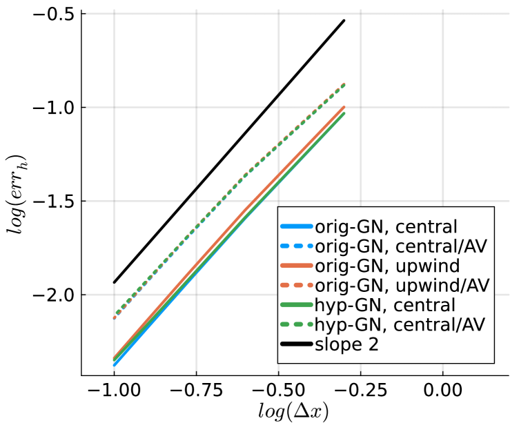
(a) Depth convergence, SBP operators of order 2.

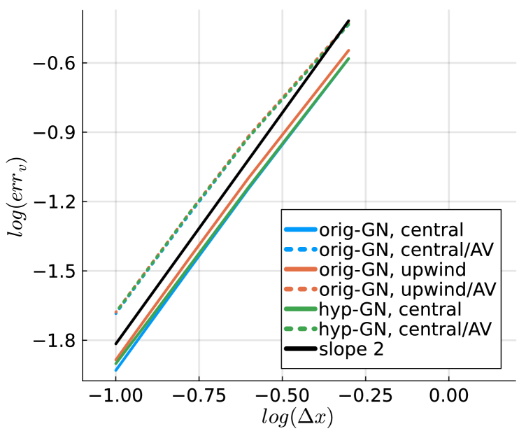
(b) Velocity convergence, SBP operators of order 2.

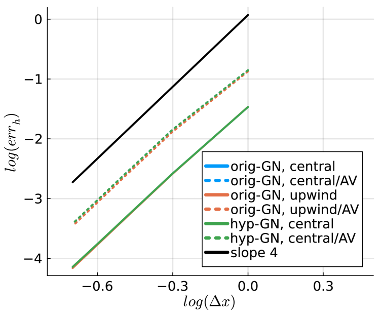
(c) Depth convergence, SBP operators of order 4.

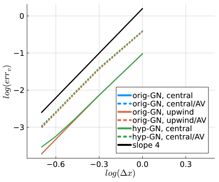
(d) Velocity convergence, SBP operators of order 4.

Figure 1: Convergence results using finite difference semidiscretizations with $\displaystyle N$ nodes applied to the solitary wave of the Serre-Green-Naghdi equations.

Figure 1 shows the errors of the numerical solutions measured with respect to the soliton solution of the Serre-Green-Naghdi equations for finite difference methods with different orders of accuracy, including methods with (high order) artificial viscosity. The EOC matches the expected order of accuracy. For this case artificial viscosity leads to an increase in the absolute value of the error by a factor in between $\displaystyle\approx$ 2–5.

Table 1: Convergence results when increasing the parameter $\displaystyle\lambda$ of the hyperbolic approximation using eighth-order finite difference semidiscretizations with $\displaystyle N=500$ nodes applied to the solitary wave of the Serre-Green-Naghdi equations.

(e) Central operators

$\displaystyle\lambda$	$\displaystyle L^{2}$ err. $\displaystyle h$	EOC $\displaystyle h$	$\displaystyle L^{2}$ err. $\displaystyle v$	EOC $\displaystyle v$
$\displaystyle 10^{2}$	2.85e-02		8.86e-02
$\displaystyle 10^{3}$	2.89e-03	0.99	8.60e-03	1.01
$\displaystyle 10^{4}$	2.91e-04	1.00	1.02e-03	0.92
$\displaystyle 10^{5}$	2.93e-05	1.00	2.45e-04	0.62
$\displaystyle 10^{6}$	2.92e-06	1.00	1.33e-04	0.26

(f) Central operators and artificial dissipation

$\displaystyle\lambda$	$\displaystyle L^{2}$ err. $\displaystyle h$	EOC $\displaystyle h$	$\displaystyle L^{2}$ err. $\displaystyle v$	EOC $\displaystyle v$
$\displaystyle 10^{2}$	2.85e-02		8.86e-02
$\displaystyle 10^{3}$	2.89e-03	0.99	8.60e-03	1.01
$\displaystyle 10^{4}$	2.91e-04	1.00	1.02e-03	0.92
$\displaystyle 10^{5}$	2.94e-05	1.00	2.45e-04	0.62
$\displaystyle 10^{6}$	3.10e-06	0.98	1.41e-04	0.24

For the hyperbolic approximation, the EOC matches the expected order of accuracy for the second-order method, when using $\displaystyle\lambda=10^{4}$. For the fourth-order method $\displaystyle\lambda=10^{6}$, is necessary to obtain the proper rates for the water height, but even with this value the convergence rates are a bit smaller for the velocity. A larger value of $\displaystyle\lambda$ may allow to correct this. For completeness we also study the convergence when increasing the value of the parameter $\displaystyle\lambda$. The results are summarized in Table 1. The EOC of the water height is unity. The velocity converges as well but with a reduced EOC, especially for large $\displaystyle\lambda$. The differences due to the artificial diffusion are very small here.

11.1.2 Manufactured solution for the hyperbolic system

We use the method of manufactured solutions to check the implementation. We choose the solution

$$h(t,x) =7+2\cos(2\pi x)+\cos(2\pi x-4\pi t),$$ (146)

$$u(t,x) =\sin(2\pi x-\pi t),$$

$$\eta(t,x) =h(t,x),$$

$$w(t,x) =-h(t,x)\partial_{x}u(t,x),$$

$$b =-5-2\cos(2\pi x),$$

and add source terms to the equations so that the equations are satisfied for the manufactured solutions. We consider the grid convergence of the error at the final time $\displaystyle t=1$ on a domain of width $\displaystyle 1$. The results shown in Figure 2 confirm the expected order of accuracy for the finite difference semidiscretizations. For this test, the difference brought by adding artificial dissipation is orders of magnitude smaller than the errors itself, and the convergence curves are essentially superposed.

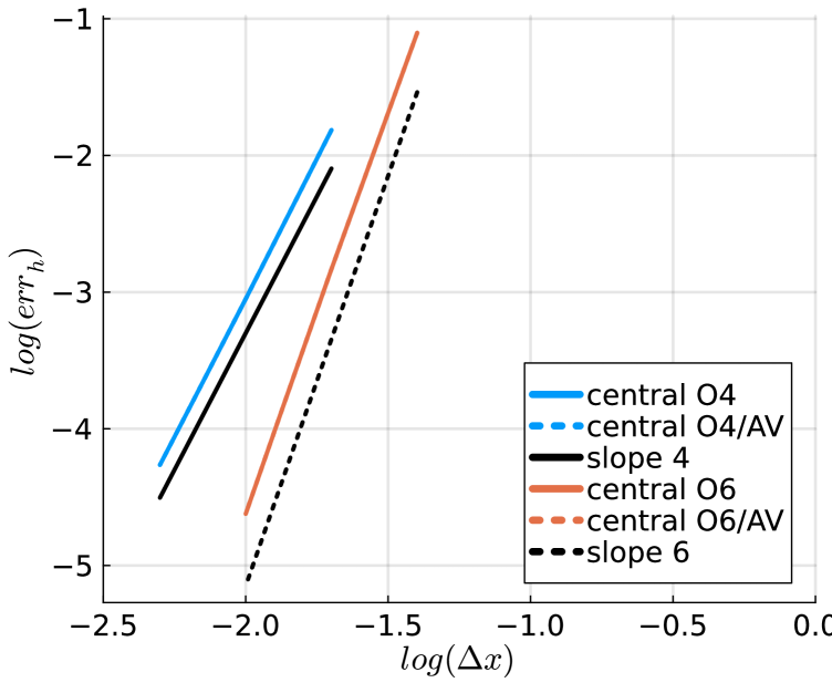
(a) Depth error convergence.

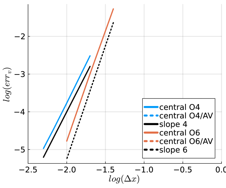
(b) Velocity error convergence.

Figure 2: Grid convergence to the manufactured solution for the hyperbolic system results using finite difference semidiscretizations of different orders and $\displaystyle\lambda=500$. Left: depth. Right: velocity.

11.2 Qualitative comparison of upwind and central methods

To point out the different behavior of upwind and central finite difference methods for solving the elliptic equations, we compare numerical results for a Gaussian initial condition.

11.2.1 Qualitative comparison: flat bathymetry

First, we consider the initial condition

$$h(x,0)=1+\exp(-x^{2}),\quad u(x,u)=10^{-2},\quad b(x)=0,$$ (147)

and discretize the domain $\displaystyle[-150,150]$ with second-order finite differences. We use the fifth-order Runge-Kutta method of [129] with tolerances $\displaystyle 10^{-5}$ for the time interval $\displaystyle[0,35]$. Reference solutions are shown in Figure 3. All the methods considered in this section are visually fully converged with the same number of nodes $\displaystyle N=3000$.

(a) Hyperbolic approximation with $\displaystyle\lambda=500$.

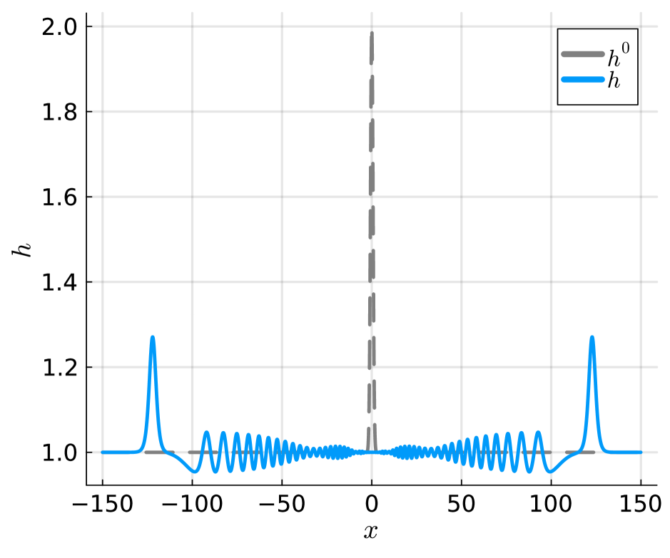
(b) Original Serre-Green-Naghdi equations.

(c) Serre-Green-Naghdi with artificial diffusion.

Figure 3: Numerical solutions for the initial condition (147). These reference solutions are all visually converged on the same grid with $\displaystyle N=3000$ nodes using second-order central finite difference methods.

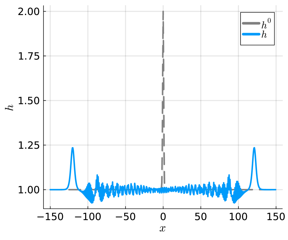
(a) Central operators.

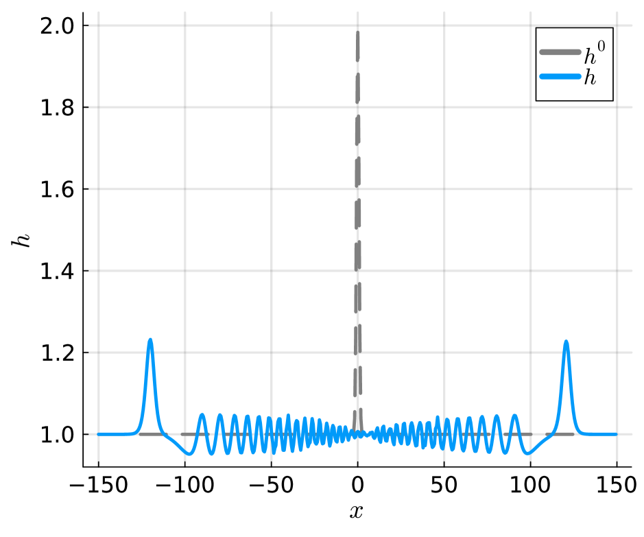
(b) Upwind operators.

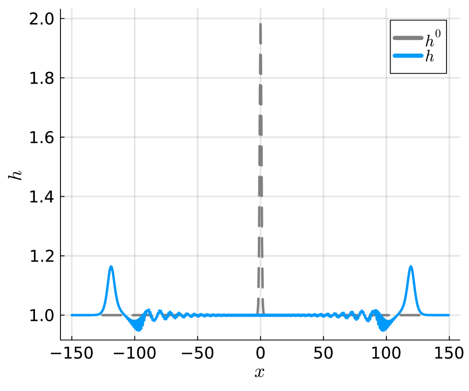
(c) Central operators plus AV.

Figure 4: Numerical solutions obtained with second-order finite difference methods with $\displaystyle N=500$ nodes for the original Serre-Green-Naghdi equations for the same setup as in Figure 3.

Next, we compare three approaches for the original Serre-Green-Naghdi equations with only $\displaystyle N=500$ nodes: central SBP operators, upwind SBP operators, and central SBP plus artificial viscosity. The results are shown in Figure 4. The central discretization of the Laplacian leads to spurious oscillations due to under-resolution. These oscillations, absent in the mesh resolved solutions, are completely removed by the upwind structure-preserving discretization. Artificial viscosity allows to remove some of the oscillations, but also damps the solution everywhere, as visible from the lower water heights obtained. This qualitative difference is in accordance with the behavior of central (wide-stencil) and upwind (narrow-stencil) discretizations of several time-dependent problems [80, 81] including other systems of dispersive wave equations [70]. For the effects of numerical dissipation one can instead refer to [60].

11.2.2 Qualitative comparison: variable bathymetry

Next, we use a variable bathymetry and

$$h(x,0)=1+\exp(-x^{2})-b(x),\quad u(x,u)=10^{-2},\quad b(x)=\frac{\cos(\pi x/75)}{4}.$$ (148)

Reference solutions are shown in Figure 5. All methods are visually converged at the same level $\displaystyle N=3000$ nodes.

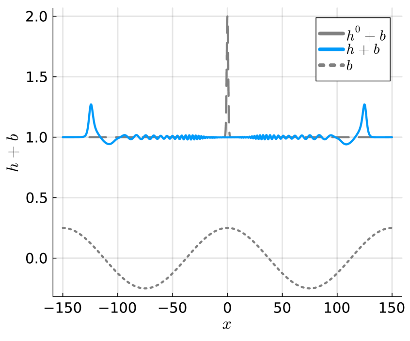
(a) Hyperbolic approximation with $\displaystyle\lambda=500$.

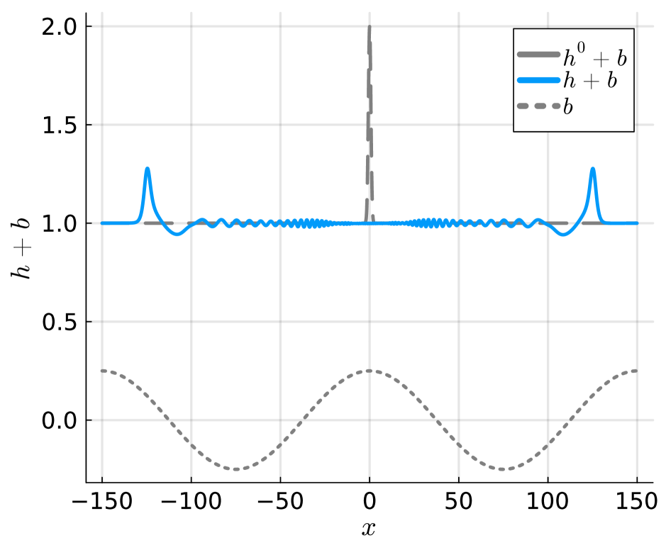
(b) Serre-Green-Naghdi equations (mild slope).

(c) Full Serre-Green-Naghdi equations.

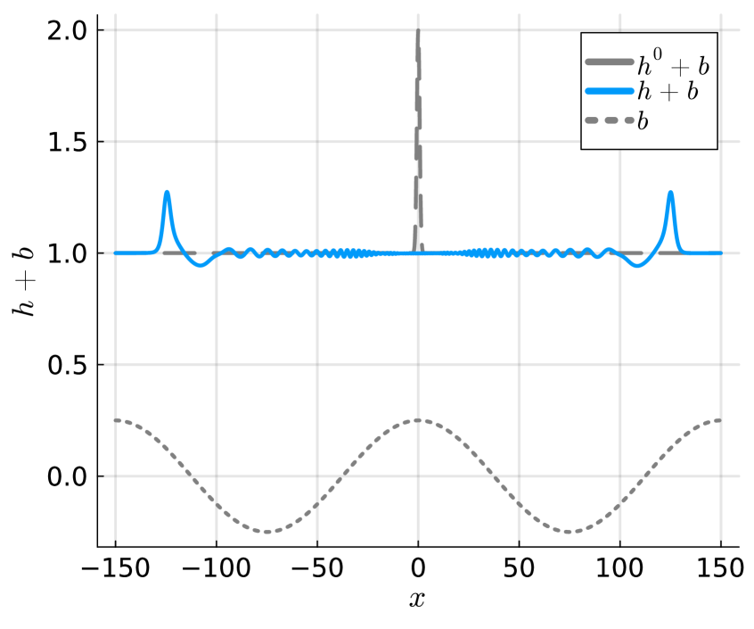
(d) Full Serre-Green-Naghdi plus artificial dissipation.

Figure 5: Numerical solutions for the initial condition (148). These reference solutions are all visually converged on the same grid with $\displaystyle N=3000$ nodes using second-order central finite difference methods.

Numerical solutions obtained with second-order finite difference methods with $\displaystyle N=500$ nodes for the original Serre-Green-Naghdi equations are shown in Figure 6. As before, the central discretization of the Laplacian leads to spurious oscillations. The oscillations are in this case removed in both the upwind SBP method, which is structure-preserving, and using artificial viscosity. However, as expected, on coarse meshes the latter has dramatic impact on the wave heights obtained, and on the resolution of secondary waves.

(a) Central operators, mild slope.

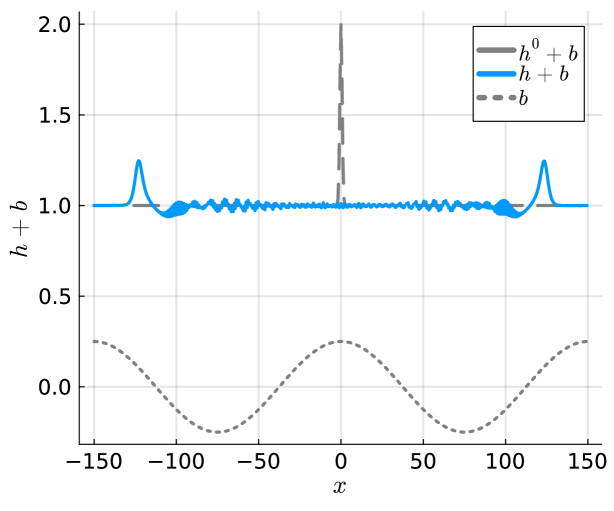
(b) Central operators, full system.

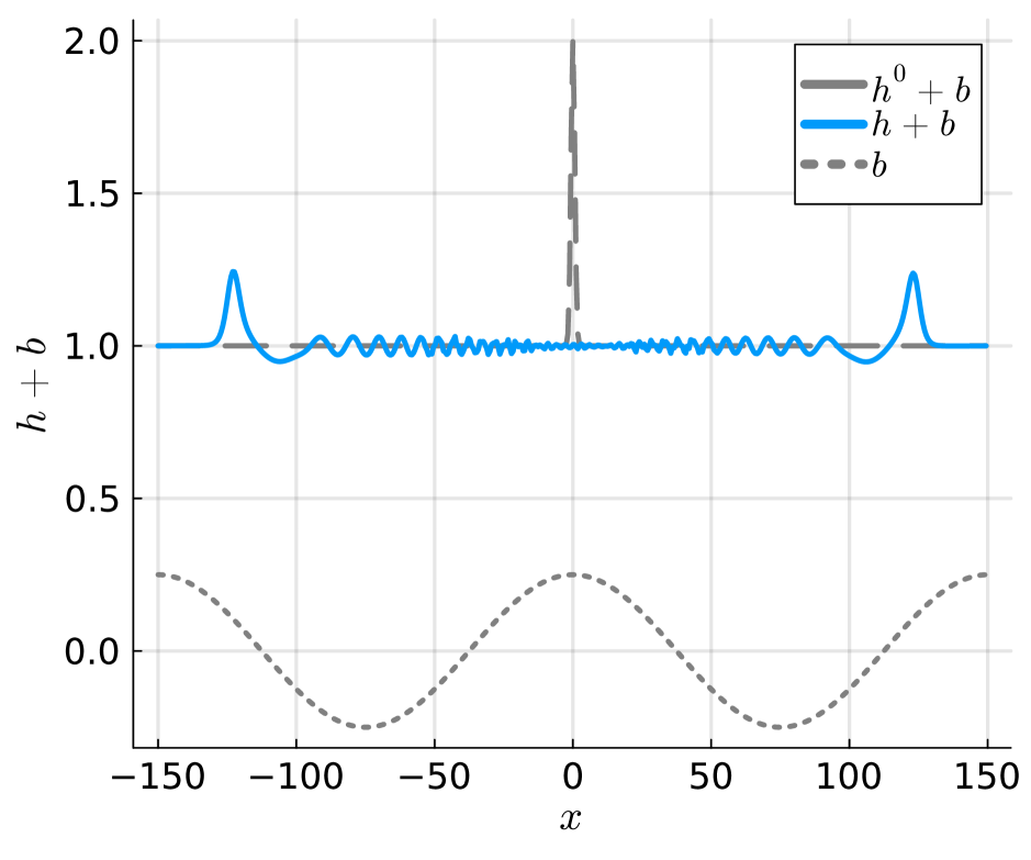
(c) Upwind operators, mild slope.

(d) Upwind operators, full system.

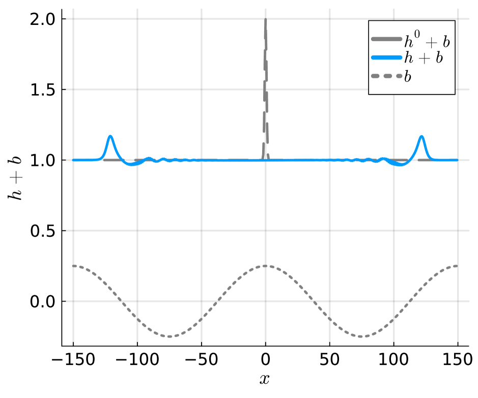
(e) Central + AV, full system.

Figure 6: Numerical solutions obtained with second-order finite difference methods with $\displaystyle N=500$ nodes for the original Serre-Green-Naghdi equations for the same setup as in Figure 5.

11.3 Conservation of invariants

In this section, we check the conservation of the invariants, i.e., the total water mass and the total energy. We use again the initial conditions and setups from Section 11.2 for constant and variable bathymetry.

11.3.1 Conservation of invariants: flat bathymetry

Table 2: Conservation of invariants (error “Er” of water mass $\displaystyle\smallint h$, momentum $\displaystyle\smallint hu$, and energy $\displaystyle\smallint E$) for constant bathymetry.

(f) Hyperbolic approximation $\displaystyle\lambda=500$.
text here

$\displaystyle\Delta t$	Er$\displaystyle\,\smallint\!h$	Er$\displaystyle\,\smallint\!hu$	Er$\displaystyle\,\smallint\!E$	EOC
0.0100	2.3e-13	1.7e-07	6.4e-06
0.0050	2.3e-13	1.7e-07	3.3e-07	4.28
0.0020	2.8e-13	1.7e-07	3.8e-09	4.88
0.0010	2.8e-13	1.7e-07	1.2e-10	4.96
0.0005	4.5e-13	1.7e-07	7.3e-12	4.05

(g) Hyperbolic approximation with $\displaystyle\lambda=500$ and AV (error of energy with orders 2 and 4).

$\displaystyle\Delta t$	Er$\displaystyle\,\smallint\!h$	Er$\displaystyle\,\smallint\!hu$	Er$\displaystyle\,\smallint\!E$
			O2	O4
0.0100	2.3e-13	1.5e-07	1.4	8.9e-02
0.0050	2.3e-13	1.5e-07	1.4	8.9e-02
0.0020	2.8e-13	1.5e-07	1.4	8.9e-02
0.0010	2.8e-13	1.5e-07	1.4	8.9e-02
0.0005	4.0e-13	1.5e-07	1.4	8.9e-02

(h) Original Serre-Green-Naghdi equations with central operators.

$\displaystyle\Delta t$	Er$\displaystyle\,\smallint\!h$	Er$\displaystyle\,\smallint\!hu$	EOC	Er$\displaystyle\,\smallint\!E$	EOC
0.150	1.1e-13	1.5e-06		2.8e-04
0.050	2.3e-13	4.1e-09	5.35	1.1e-06	5.06
0.020	2.8e-13	5.4e-11	4.73	1.4e-08	4.76
0.010	4.5e-13	1.8e-12	4.95	4.4e-10	4.94
0.005	7.4e-13	3.5e-14	5.65	2.0e-11	4.43

(i) Original Serre-Green-Naghdi equations with central operators and AV (error of energy with orders 2 and 4).

$\displaystyle\Delta t$	Er$\displaystyle\,\smallint\!h$	Er$\displaystyle\,\smallint\!hu$	EOC	Er$\displaystyle\,\smallint\!E$
				O2	O4
0.150	1.1e-13	8.2e-07		1.4	8.7e-02
0.050	1.7e-13	2.7e-09	5.19	1.4	8.8e-02
0.020	2.8e-13	3.4e-11	4.77	1.4	8.8e-02
0.010	4.5e-13	1.1e-12	4.96	1.4	8.8e-02
0.005	7.4e-13	4.1e-14	4.76	1.4	8.8e-02

(j) Original Serre-Green-Naghdi equations with upwind operators.

$\displaystyle\Delta t$	Er$\displaystyle\,\smallint\!h$	Er$\displaystyle\,\smallint\!hu$	EOC	Er$\displaystyle\,\smallint\!E$	EOC
0.150	1.1e-13	1.7e-05		2.1e-04
0.050	2.3e-13	1.2e-08	6.57	9.7e-07	4.88
0.020	2.8e-13	9.8e-11	5.27	1.2e-08	4.78
0.010	4.0e-13	4.4e-12	4.46	4.0e-10	4.95
0.005	7.4e-13	1.7e-13	4.69	1.9e-11	4.39

(k) Original Serre-Green-Naghdi equations with upwind operators and AV (error of energy with orders 2 and 4).

$\displaystyle\Delta t$	Er$\displaystyle\,\smallint\!h$	Er$\displaystyle\,\smallint\!hu$	EOC	Er$\displaystyle\,\smallint\!E$
				O2	O4
0.150	2.3e-13	1.4e-05		1.3	8.1e-02
0.050	2.3e-13	1.1e-08	6.50	1.3	8.1e-02
0.020	3.4e-13	4.4e-11	6.03	1.3	8.1e-02
0.010	4.0e-13	2.5e-12	4.12	1.3	8.1e-02
0.005	6.8e-13	9.5e-14	4.73	1.3	8.1e-02

The conservation of mass, momentum, and energy is measured on the test of Section 11.2. We use second-order finite differences with $\displaystyle N=1000$ nodes, in the spatial domain $\displaystyle[-150,150]$, on the time interval $\displaystyle t\in[0,35]$. The results are shown in Table 2. For all systems, the linear invariant (total water mass) is conserved up to machine accuracy. For the structure-preserving semidiscretizations, the total energy error decreases with the time step size, and the EOC matches the order of accuracy of the time integration method. This is expected since, being a nonlinear invariant, total energy is not conserved exactly by the time integration method. For the original systems we obtain the same result for the momentum, which is a nonlinear invariant due to the formulation using $\displaystyle hu_{t}$. As already said, this could be avoided working with $\displaystyle(hu)_{t}$ but with considerable overheads in the solution of the elliptic problem. In any case, the momentum EOC matches the order of accuracy of the time discretization. Conversely, the momentum error for the hyperbolic approximation is the same for all $\displaystyle\Delta t$s since in this case the semidiscretization in space is non momentum conserving. The results including AV show a finite defect in the energy integral, independent of the time step. This error is given by $\displaystyle\smallint\mu(\Delta x,p)h(u_{x})^{2}$ at the final time, and reduces when passing from order 2 to order 4 as shown in the tables.

11.3.2 Conservation of invariants: variable bathymetry

Next, we use a variable bathymetry as in (148). The other parameters are still the same as before. The results shown in Table 3 show similar behavior to the constant bathymetry case. To save space we do note report here the errors when including artificial dissipation, which also behave very similarly as in the previous sub-section. We do report a table with the energy errors at final time $\displaystyle t=35$ for second- and fourth-order schemes showing some small dependence of the error on the formulation, but again mostly on the order (and mesh).

Table 3: Conservation of invariants (errors “Er” of water mass $\displaystyle\smallint h$ and energy $\displaystyle\smallint E$) for variable bathymetry. The spatial discretizations use second-order finite differences with $\displaystyle N=1000$ nodes in the interval $\displaystyle[-150,150]$.

(l) Conservation of energy for second- and fourth-order finite difference schemes with AV.

Formulation	Er$\displaystyle\,\smallint\!E$
	O2	O4
Hyp. $\displaystyle\lambda=500$	1.20	7.49e-02
Orig. mild slope central	1.20	7.27e-02
Orig. mild slope upwind	1.19	7.27e-02
Orig. full central	1.20	7.27e-02
Orig. full upwind	1.19	7.27e-02

(m) Hyperbolic approximation with $\displaystyle\lambda=500$.
text here

$\displaystyle\Delta t$	Er $\displaystyle\smallint h$	Er $\displaystyle\smallint E$	EOC
0.0100	2.3e-13	6.5e-06
0.0050	2.3e-13	3.8e-07	4.12
0.0020	2.3e-13	4.4e-09	4.87
0.0010	3.4e-13	1.4e-10	4.97
0.0005	2.8e-13	5.5e-12	4.68

(n) Serre-Green-Naghdi equations (mild slope) with central operators.

$\displaystyle\Delta t$	Er $\displaystyle\smallint h$	Er $\displaystyle\smallint E$	EOC
0.150	2.3e-13	8.9e-04
0.050	2.3e-13	1.4e-06	5.84
0.020	2.3e-13	2.1e-08	4.62
0.010	2.3e-13	6.9e-10	4.93
0.005	2.8e-13	2.2e-11	4.97

(o) Serre-Green-Naghdi equations (mild slope) with upwind operators.

$\displaystyle\Delta t$	Er $\displaystyle\smallint h$	Er $\displaystyle\smallint E$	EOC
0.150	1.7e-13	6.5e-04
0.050	2.3e-13	1.2e-06	5.70
0.020	2.3e-13	1.7e-08	4.65
0.010	2.3e-13	5.7e-10	4.94
0.005	2.3e-13	1.9e-11	4.94

(p) Full Serre-Green-Naghdi equations with central operators.

$\displaystyle\Delta t$	Er $\displaystyle\smallint h$	Er $\displaystyle\smallint E$	EOC
0.150	2.3e-13	8.9e-04
0.050	2.3e-13	1.4e-06	5.84
0.020	2.3e-13	2.1e-08	4.62
0.010	2.3e-13	6.9e-10	4.94
0.005	3.4e-13	2.2e-11	4.94

(q) Full Serre-Green-Naghdi equations with upwind operators.

$\displaystyle\Delta t$	Er $\displaystyle\smallint h$	Er $\displaystyle\smallint E$	EOC
0.150	1.7e-13	6.5e-04
0.050	2.3e-13	1.2e-06	5.70
0.020	2.3e-13	1.7e-08	4.65
0.010	2.3e-13	5.7e-10	4.93
0.005	2.8e-13	1.9e-11	4.89

11.4 Well-balancedness

We also check the well-balancedness of the methods. For this, we use the initial condition

$$h(x,0)=1-b(x),\quad u(x,u)=0,\quad b(x)=\frac{\cos(\pi x/75)}{4},$$ (149)

in the interval $\displaystyle[-150,150]$ with $\displaystyle N=1000$ nodes. We report in Table 4 the results obtained without artificial viscosity. The ones obtained with this term added are identical down to machine accuracy and are omitted to save space. The results shown confirm the well-balancedness of the semidiscretizations.

Table 4: Discrete $\displaystyle L^{2}$ norm of the ODE RHS for the well-balancedness test case discretized with central finite difference methods of different orders of accuracy $\displaystyle p$.

(r) Hyperbolic approximation with $\displaystyle\lambda=500$.

Order $\displaystyle p$	$\displaystyle h$	$\displaystyle v$	$\displaystyle w$	$\displaystyle\eta$
2	0.0e+00	1.9e-14	0.0e+00	0.0e+00
4	0.0e+00	2.6e-14	0.0e+00	0.0e+00
6	0.0e+00	3.0e-14	0.0e+00	0.0e+00

(s) Hyperbolic approximation with $\displaystyle\lambda=5000$.

Order $\displaystyle p$	$\displaystyle h$	$\displaystyle v$	$\displaystyle w$	$\displaystyle\eta$
2	0.0e+00	1.9e-14	0.0e+00	0.0e+00
4	0.0e+00	2.6e-14	0.0e+00	0.0e+00
6	0.0e+00	3.0e-14	0.0e+00	0.0e+00

(t) Mild slope Serre-Green-Naghdi, central operators

$\displaystyle p$	$\displaystyle h$	$\displaystyle v$
2	0.0e+00	5.2e-15
4	0.0e+00	5.5e-15
6	0.0e+00	5.9e-15

(u) Mild slope Serre-Green-Naghdi, upwind operators

$\displaystyle p$	$\displaystyle h$	$\displaystyle v$
2	0.0e+00	4.2e-15
4	0.0e+00	5.0e-15
6	0.0e+00	5.2e-15

(v) Full Serre-Green-Naghdi, central operators

$\displaystyle p$	$\displaystyle h$	$\displaystyle v$
2	0.0e+00	5.2e-15
4	0.0e+00	5.5e-15
6	0.0e+00	5.9e-15

(w) Full Serre-Green-Naghdi, upwind operators

$\displaystyle p$	$\displaystyle h$	$\displaystyle v$
2	0.0e+00	4.2e-15
4	0.0e+00	5.0e-15
6	0.0e+00	5.2e-15

11.5 Error growth of solitons of the Serre-Green-Naghdi equations

We study the error growth in long-time simulations of solitary waves. We use the setup of Section 11.1.1, and apply Fourier pseudospectral methods in space with $\displaystyle N=2^{7}$ nodes. We choose the final time such that the soliton has traveled through the domain 20 times. We solve the nonlinear scalar equation for relaxation to conserve the energy using the ITP method [91]. The results are shown in Figure 7. Energy is only conserved exactly with relaxation, and in this case it is conserved up to the accuracy of the nonlinear scalar solver. In this case we also see a linear growth in time of the error, while the error of the baseline structure-preserving method grows quadratically. This behavior has also been observed for other nonlinear dispersive systems [23, 28, 108]. It can be explained using the theory of relative equilibrium solutions [27]: the SGN equations can be expressed as Hamiltonian system [75] with the total energy as Hamiltonian $\displaystyle\mathcal{H}$. However, there is another invariant $\displaystyle\mathcal{Q}$ of the SGN equations and solitary wave solutions are critical points of the functional $\displaystyle\mathcal{H}-c\mathcal{Q}$ [75]. Thus, the basic structure of relative equilibrium solutions of [27] is satisfied and we can expect a quadratic error growth for general time integration methods and a linear error growth for methods conserving the total energy.

(a) Error without relaxation.

(b) Error with relaxation.

(c) Energy without relaxation.

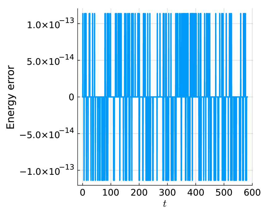
(d) Energy with relaxation.

Figure 7: Long-time soliton propagation for the Serre-Green-Naghdi equations. Energy-conserving Fourier pseudospectral methods, and fifth-order Runge-Kutta method of [129] with and without relaxation to conserve the energy. Top: discrete $\displaystyle L^{2}$ errors of the numerical solutions. Bottom: energy error after 20 periods.

11.6 Riemann problem

We consider a Riemann problem following the setup by [126]. We use a smoothed initial profile

$$h(x,0)=h_{R}+\dfrac{h_{L}-h_{R}}{2}\bigl{(}1-\tanh(x/\alpha)\bigr{)},\quad u(x,0)=0,$$ (150)

with $\displaystyle\alpha=2$. The analysis of Riemann invariants of the shallow-water system, coupled with the analysis of the Whitham system for the SGN equations [31, 49, 126, 33] allow to recover the approximate values $\displaystyle(h^{*},u^{*})$ of the mean flow dividing the rarefaction wave and the dispersive shock zones as

$$h^{*}=\dfrac{(\sqrt{h_{L}}+\sqrt{h_{R}})^{2}}{4},\quad u^{*}=2(\sqrt{gh^{*}}-\sqrt{gh_{R}}),\quad a^{+}=\delta_{0}-\dfrac{1}{12}\delta_{0}^{2}+O(\delta_{0}^{3}),$$ (151)

where $\displaystyle a^{+}$ is the second-order asymptotic approximation of the amplitude of the leading soliton and $\displaystyle\delta_{0}=|h_{R}-h_{L}|$. We take $\displaystyle h_{L}=1.8$ and $\displaystyle h_{R}=1.0$, and solve the problem until time $\displaystyle t=47.434$ on a large domain $\displaystyle[-600,600]$. Only the results in the interval $\displaystyle[-300,300]$ are retained. Figure 8 shows solutions for the hyperbolic approximation and the original SGN equations obtained with structure-preserving central finite difference operators. The results from the two systems agree very well with each other, the analytical predictions, and the numerical results of [49, 97].

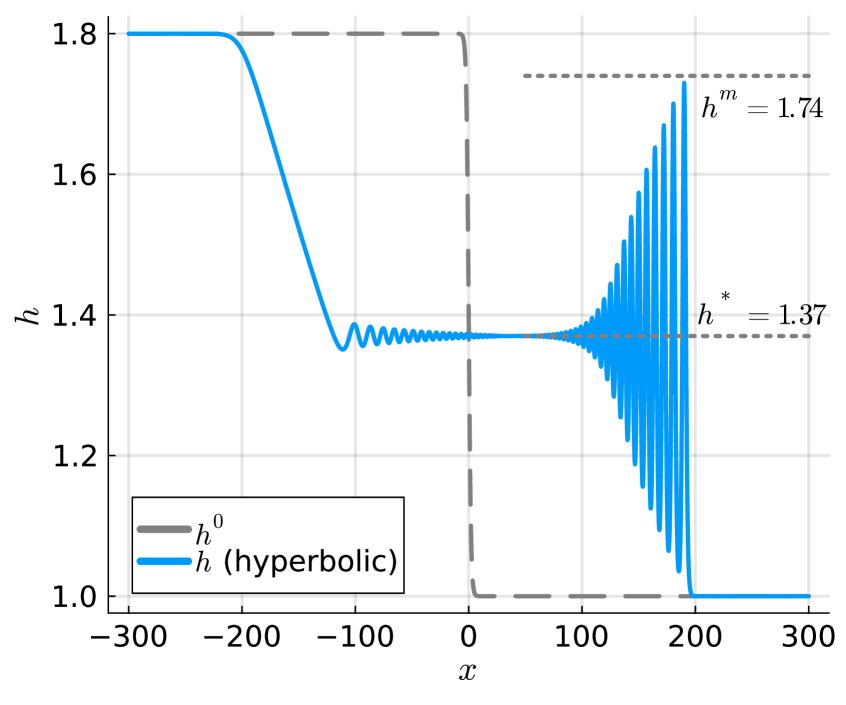
(a) Hyperbolic approximation with $\displaystyle\lambda=500$.

(b) Serre-Green-Naghdi equations.

Figure 8: Riemann problem using structure-preserving second-order finite differences with $\displaystyle\Delta x=0.3$. The intermediate water height $\displaystyle h^{*}=1.37$ and amplitude $\displaystyle h^{m}=1.74$ of the leading dispersive wave are in accordance with analytical predictions and numerical results [49, 97].

11.7 Soliton fission

Next, we study the long-time behavior of a dispersive shock wave. We use the initial condition

$$h(x,0)=\begin{cases}1.8,&|x|<1,\\ 1.0,&\text{otherwise},\end{cases}\quad u(x,0)=0,$$ (152)

and discretize the spatial domain $\displaystyle[-500,500]$ with $\displaystyle 10^{3}$ nodes using central second-order finite differences. We integrate the numerical solutions until $\displaystyle t=118$, and analyze the leading waves in the interval $\displaystyle[390,500]$. We take the values where the water height $\displaystyle h$ is greater than a threshold of $\displaystyle 1.001$ and fit analytical Serre-Green-Naghdi solitons to them. For this, we take the median of the remaining values of $\displaystyle h$ as baseline and use a Nelder-Mead method [86, 46] implemented in Optim.jl/Optimization.jl [85, 26] to compute a least-squares solution.

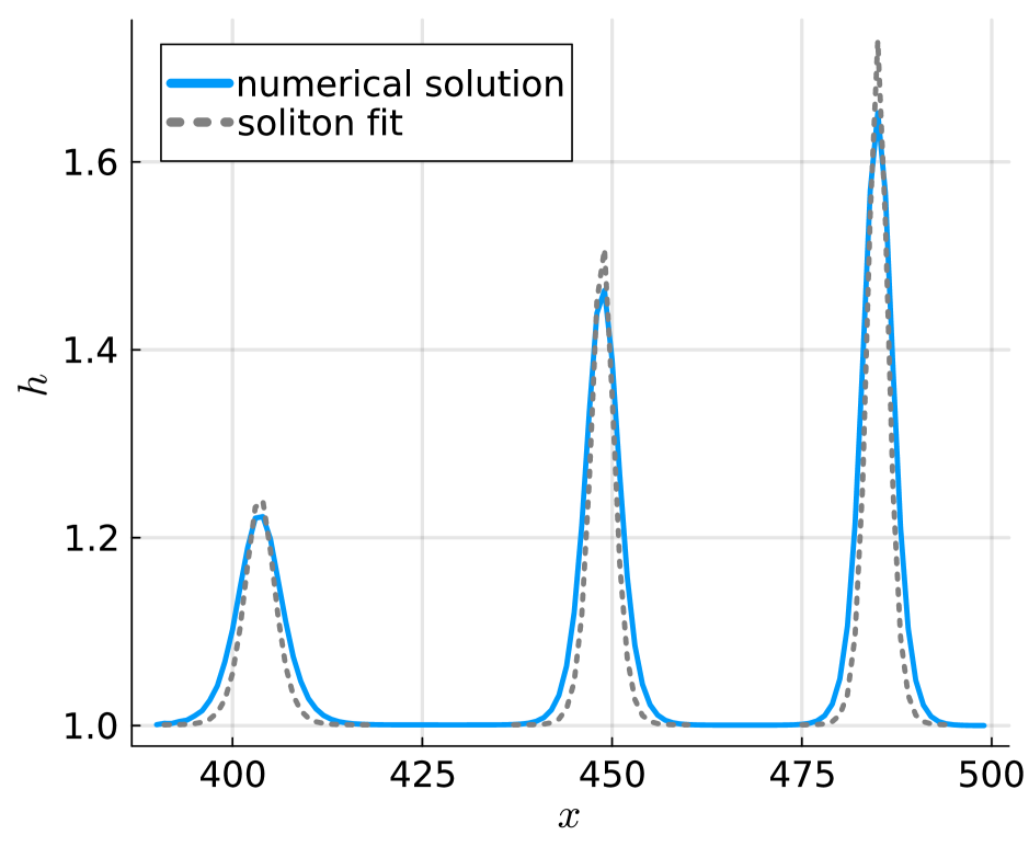
(a) Hyperbolic with $\displaystyle\lambda=500$.

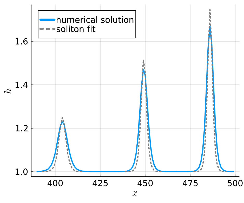
(b) Serre-Green-Naghdi equations.

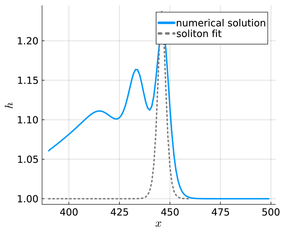
(c) Serre-Green-Naghdi + AV.

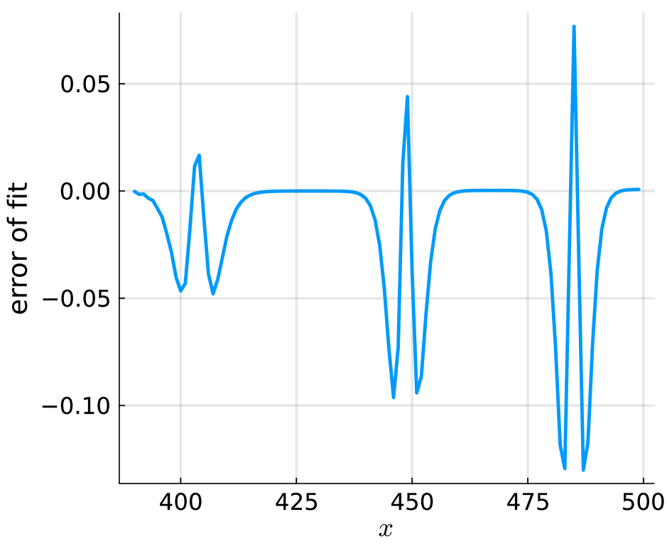
(d) Hyperbolic with $\displaystyle\lambda=500$.

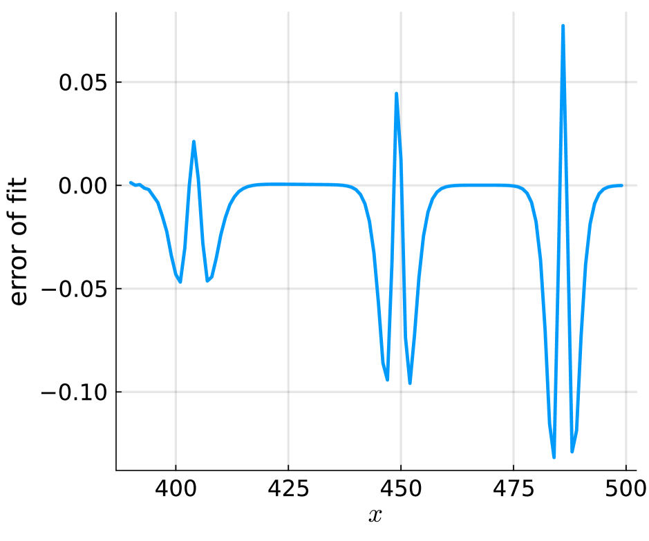
(e) Serre-Green-Naghdi equations.

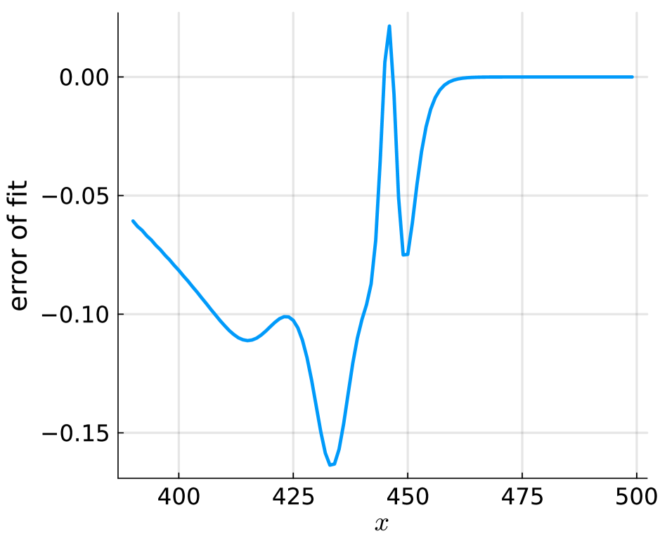
(f) Serre-Green-Naghdi + AV.

Figure 9: Leading soliton waves obtained from the rectangular initial condition discretized with second-order finite differences with $\displaystyle\Delta x=1$. Left: hyperbolic approximation with $\displaystyle\lambda=500$. Center: original Serre-Green-Naghdi model. Right: original Serre-Green-Naghdi model with numerical dissipation. Top: water height and soliton fits. Bottom: soliton fit error.

The results are shown in Figure 9. For both the hyperbolic approximation and the discretization of the original SGN equations, the numerical solutions agree very well with the fitted analytical soliton waves. The differences between the numerical solutions and the fits are roughly two orders of magnitude smaller than the amplitude of the waves. To show the impact of numerical viscosity on such long-time computations, we also plot the results of the the original SGN equations plus artificial diffusion. The corresponding results with the hyperbolic model are visually identical. We can see that not only the height of the first wave is much underestimated, but also its position, certainly due to the dependence of the celerity of the leading wave on its amplitude. The optimization method does recognize a half soliton shape in the leading front. This behaviour is further investigated and commented in the following section.

11.8 Favre waves

The propagation of undular bores, also known as Favre waves, is a classical problem, see, e.g., [131, 17] and references therein, for which well-known experiments exist [36, 128]. The initial setup considered here follows, e.g., [17, 60]. The initial solution is obtained by a smoothed discontinuity (cf. also Figure 10)

$$h(x,t=0)\mathrel{\mathop{\mathchar 58\relax}}=h_{0}+\dfrac{[\![h]\!]}{2}\left\{1-\tanh\bigg{(}\dfrac{x-x_{0}}{\alpha}\bigg{)}\right\},$$

$$u(x,t=0)\mathrel{\mathop{\mathchar 58\relax}}=u_{0}+\dfrac{[\![u]\!]}{2}\left\{1-\tanh\bigg{(}\dfrac{x-x_{0}}{\alpha}\bigg{)}\right\},$$

where

$$[\![h]\!]\mathrel{\mathop{\mathchar 58\relax}}=\varepsilon h_{0},$$

with $\displaystyle\varepsilon$ the nonlinearity, and with $\displaystyle[\![u]\!]$ satisfying the shallow-water Rankine-Hugoniot relations, and in particular

$$[\![u]\!]=\sqrt{g\dfrac{h_{1}+h_{0}}{2h_{0}h_{1}}}[\![h]\!].$$

We refer the reader to [17, 60] for further details on the setup.

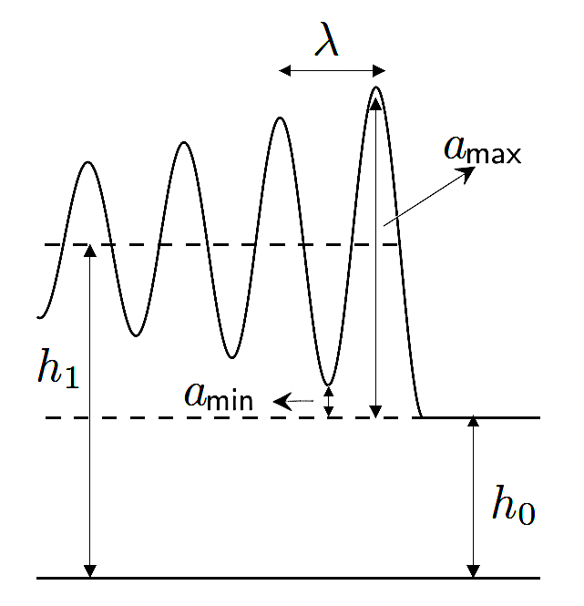
Figure 10: Favre waves: undular bore sketch, and definition of amplitudes $\displaystyle a_{\mathrm{min/max}}$ and wavelength $\displaystyle\lambda$.

As in [17, 60] we consider at first the short-time bore evolution for three values of the non-linearity $\displaystyle\varepsilon\in\{0.1,\,0.2,\,0.3\}$. The free-surface elevation for different values of the dimensionless time $\displaystyle\tilde{t}\mathrel{\mathop{\mathchar 58\relax}}=t\sqrt{g/h_{0}}$ is compared to fully nonlinear potential solutions from [131]. The results obtained with fourth-order structure-preserving finite differences on a relatively coarse mesh with $\displaystyle\Delta x=0.125$ are shown in Figures 11 and 12. Our results compare well with the fully nonlinear potential solutions, and to those of [17]. For larger values like $\displaystyle\varepsilon=0.3$ some limitations, related to the weakly dispersive character of the model itself, can be seen. The value $\displaystyle\lambda=500$ seems again large enough for the hyperbolic approximation and the original formulations to give visually indistinguishable results. For completeness, we also report in each picture the results obtained with artificial viscosity. For these short-time simulations we cannot see any impact of numerical dissipation.

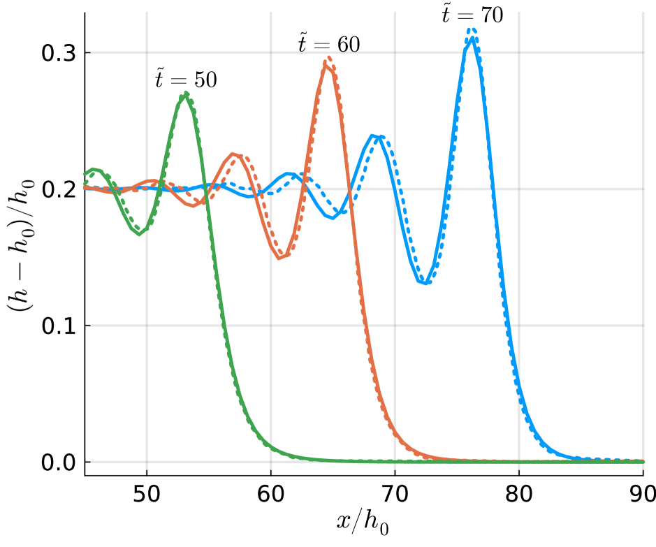
Figure 11: Favre wave: hyperbolic formulation with $\displaystyle\lambda=500$, and grid spacing $\displaystyle\Delta x=0.125$. Numerical solutions (solid lines) with nonlinearity $\displaystyle\varepsilon=0.1$ (left), $\displaystyle\varepsilon=0.2$ (center), and $\displaystyle\varepsilon=0.3$ (right). Top: energy-conservative fourth-order finite differences with central operators. Bottom: fourth-order finite differences with central operators and artificial viscosity. The dashed lines show the fully nonlinear potential solutions from [131].

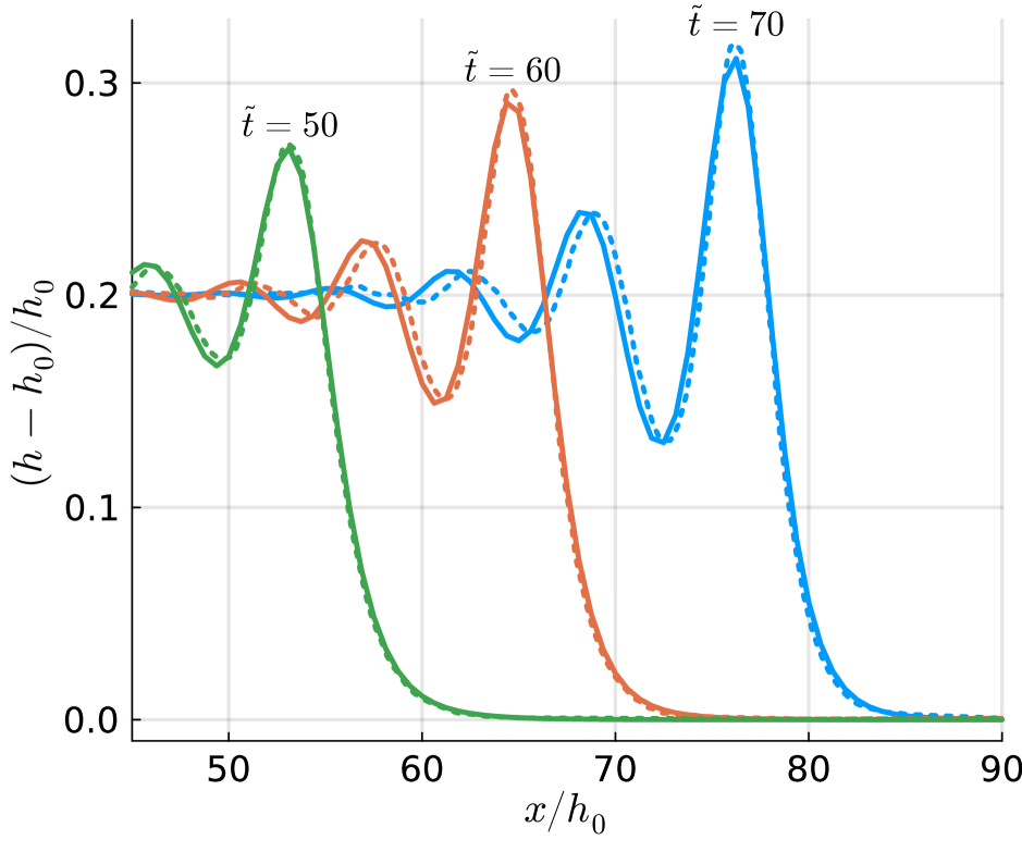
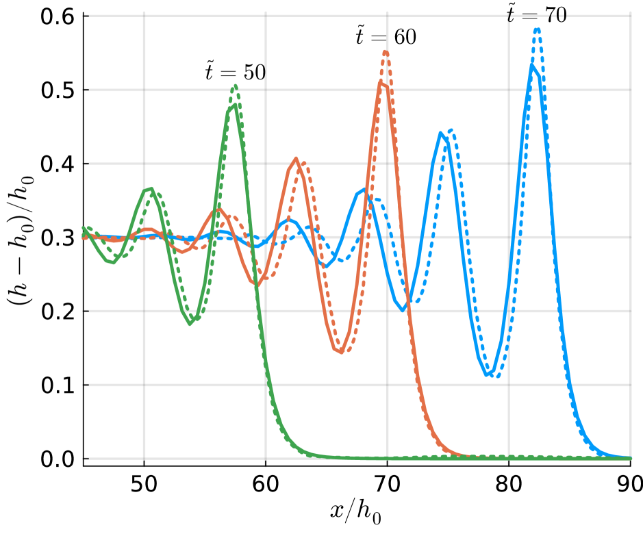
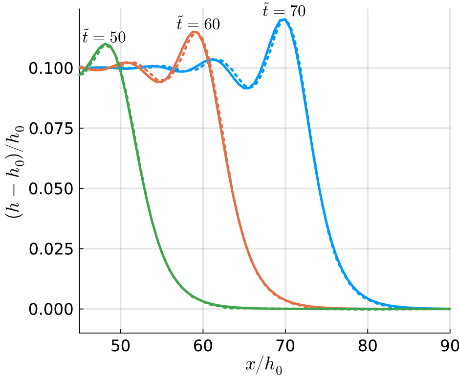
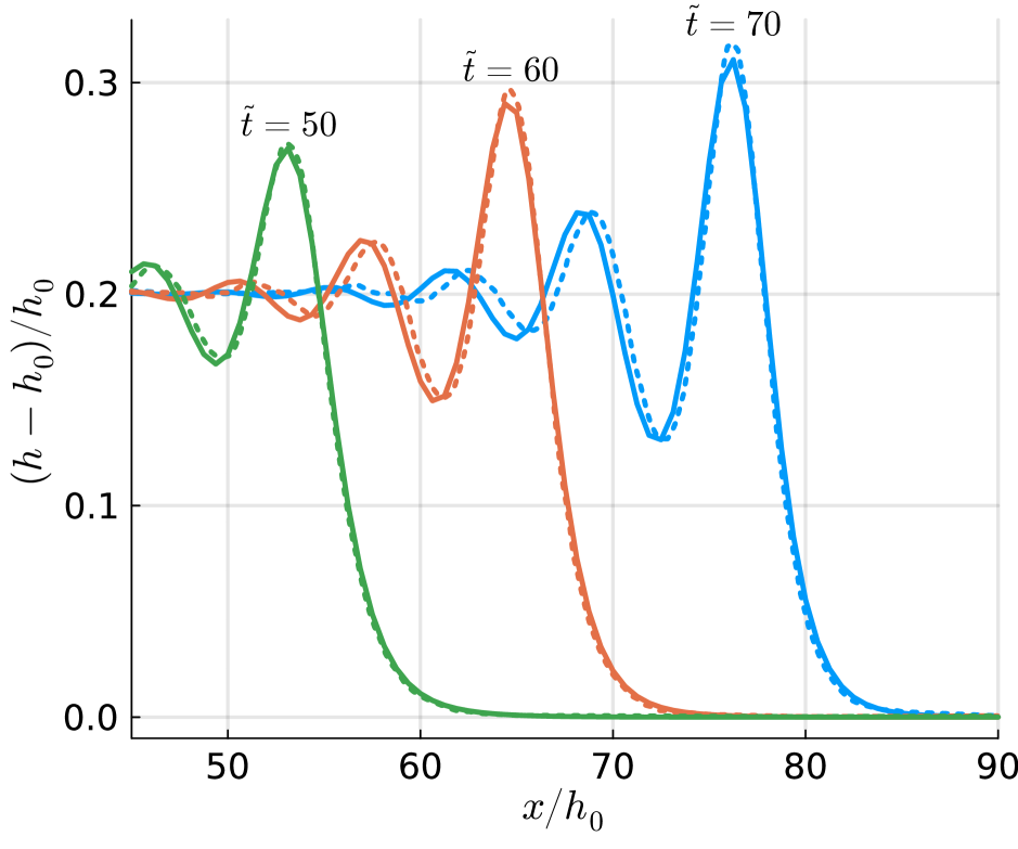
Figure 12: Favre wave: original SGN system, and grid spacing $\displaystyle\Delta x=0.125$. Numerical solutions (solid lines) with nonlinearity $\displaystyle\varepsilon=0.1$ (left), $\displaystyle\varepsilon=0.2$ (center), and $\displaystyle\varepsilon=0.3$ (right). Top : energy-conservative fourth-order finite differences with central operators. Bottom : fourth-order finite differences with central operators and artificial viscosity. The dashed lines show the fully nonlinear potential solutions from [131].

11.8.1 Long-time propagation

As shown in [60, 12, 8] this problem is extremely sensitive to the presence of dissipative processes such as friction or viscous regularization. In absence of dissipation, soliton fission occurs. Dissipation generates undular bores of lower amplitudes and finite wavelength. This fact is also known, for simpler models such as KdV and BBM, from the modulation theory [32]. As it turns out, numerical dissipation plays exactly the same role, which may lead to gross underestimations of the wave heights on coarse meshes as the results in [60] demonstrate.

To investigate this aspect we consider the propagation for a large dimensionless time $\displaystyle\tilde{t}=1500$. To save space we only consider the solution of the system in its original formulation, but similar conclusion are obtained when solving the hyperbolic approximation. The spatial domain considered is now $\displaystyle[-3000,\,3000]$ and the initial discontinuity is set at $\displaystyle x_{0}=-1000$. We plot two sets of results using second- and fourth-order schemes. The bore front is visualized in Figures 13 for second-order schemes, and 14 for fourth-order ones. From these figures we can see that the first solitary wave is already resolved on the coarsest mesh for the structure-preserving schemes. In the second-order case, a phase error is observed for the secondary waves, as one might expect due to the impact of discrete dispersion. However, the amplitudes are close to the finer mesh solution.

The fourth-order structure-preserving schemes have already resolved the solution on the coarsest mesh. The schemes with artificial viscosity behave much like in presence of a viscous regularization [12, 8], with much lower amplitudes and no fission of solitons. In the fourth-order case, doubling the number of nodes allows to obtain a reasonable prediction of wave height and position. In the second-order case even with two refinements the dissipative method still provides large amplitude underestimations.

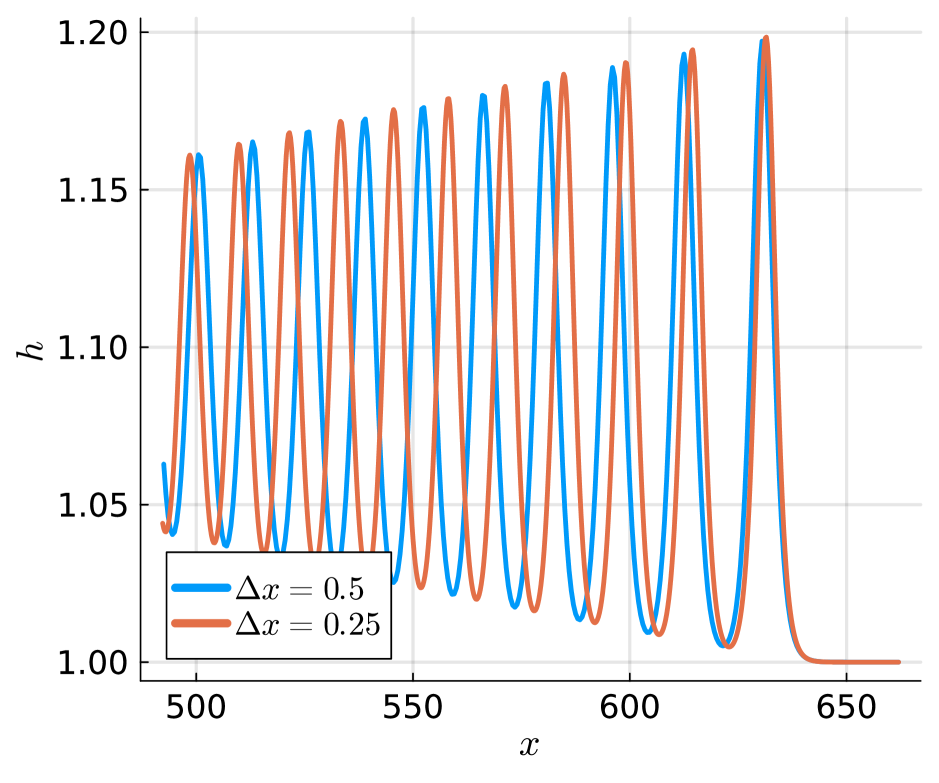
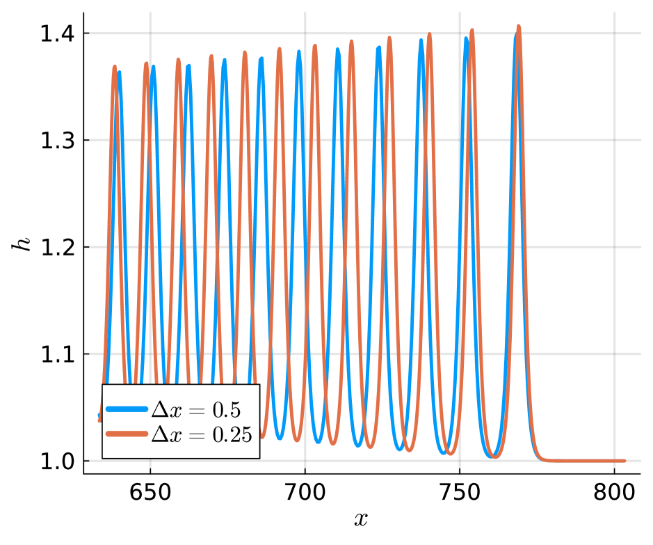
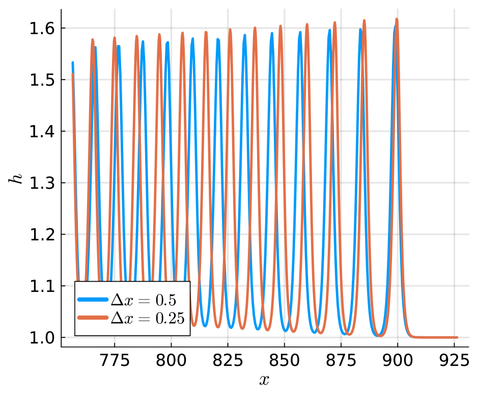
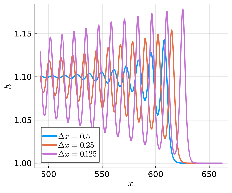
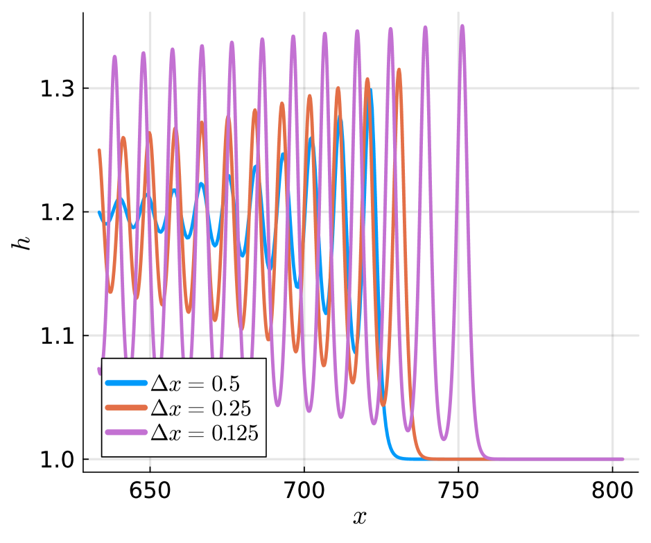
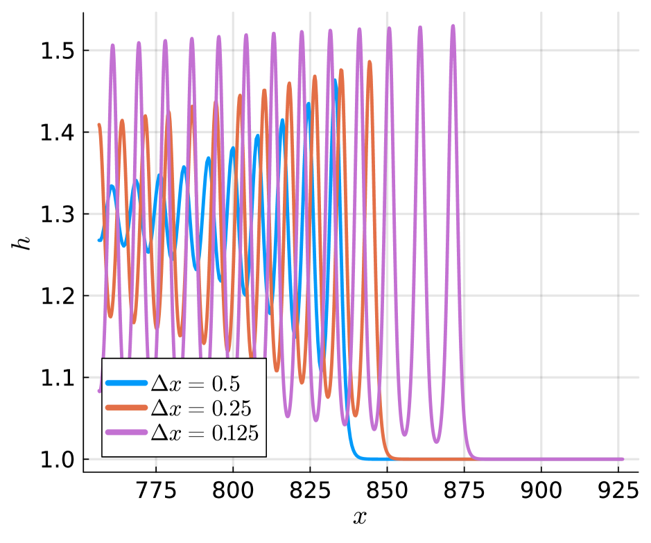
Figure 13: Favre waves. Solutions of the original SGN system at dimensionless time $\displaystyle\tilde{t}=1500$ for nonlinearities $\displaystyle\varepsilon=0.1$ (left), $\displaystyle\varepsilon=0.2$ (center), and $\displaystyle\varepsilon=0.3$ (right). Top: structure-preserving second-order finite difference scheme. Bottom: second-order finite difference with artificial viscosity.

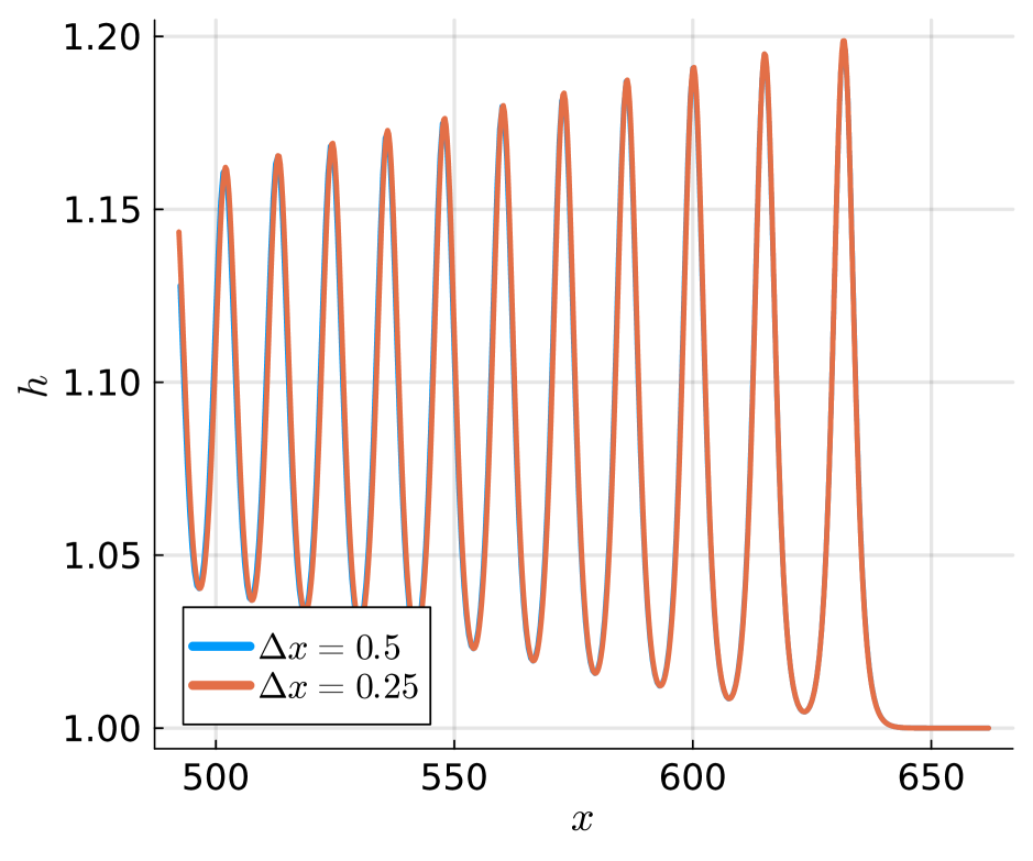
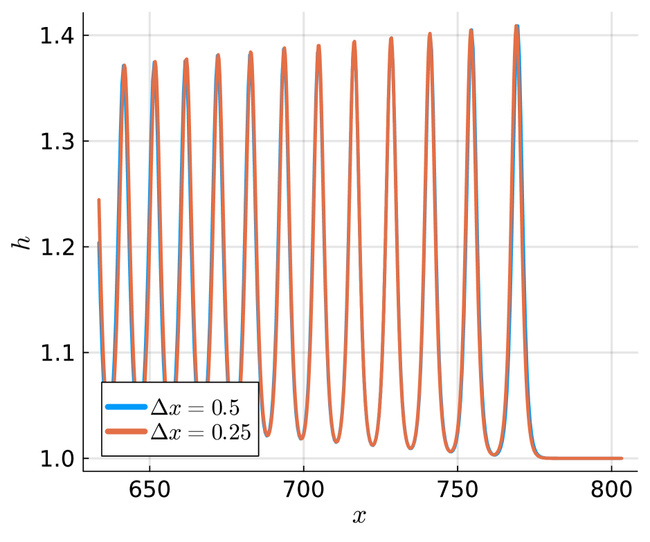
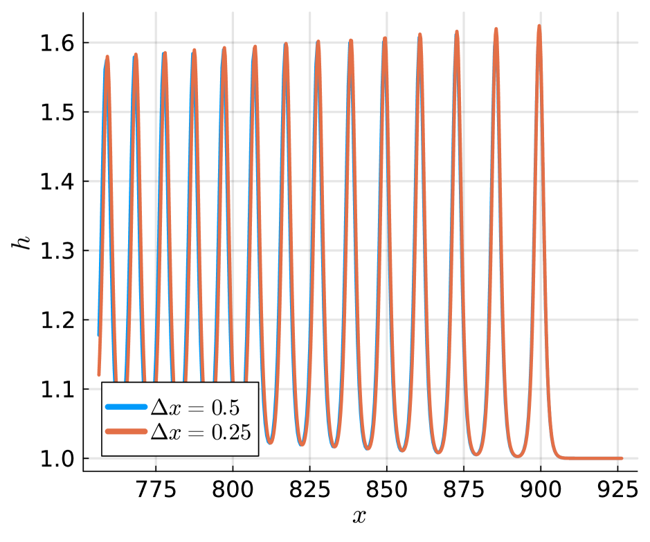
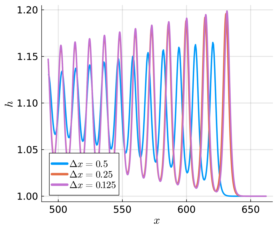
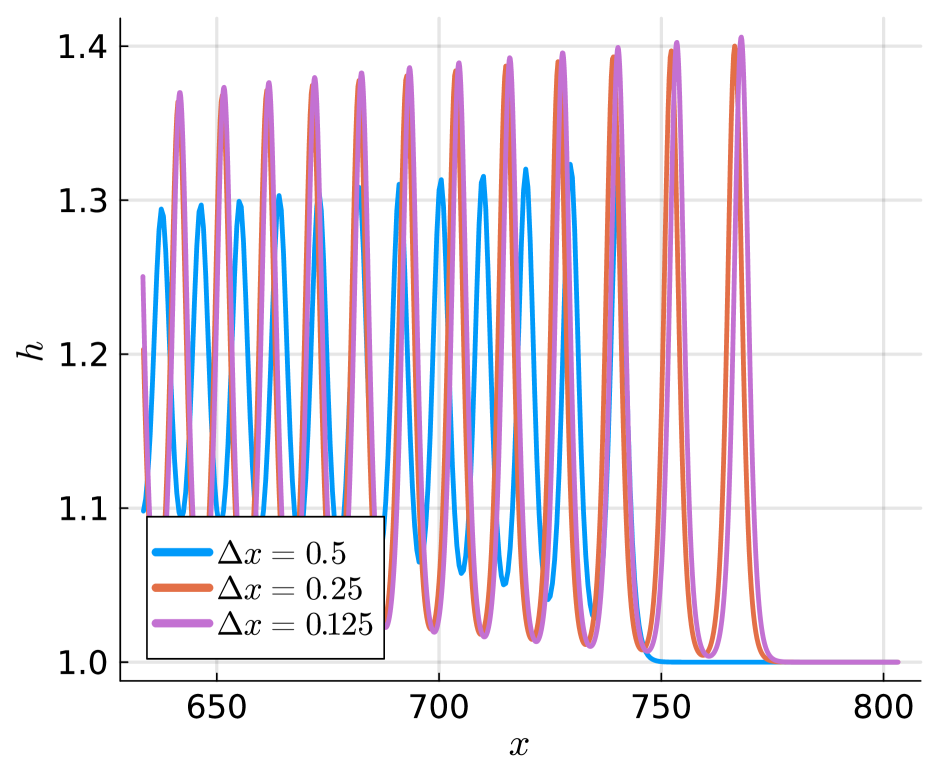
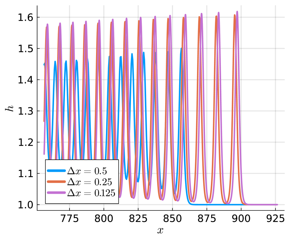
Figure 14: Favre waves. Solutions of the original SGN system at dimensionless time $\displaystyle\tilde{t}=1500$ for nonlinearities $\displaystyle\varepsilon=0.1$ (left), $\displaystyle\varepsilon=0.2$ (center), and $\displaystyle\varepsilon=0.3$ (right). Top: structure-preserving fourth-order finite difference scheme. Bottom: fourth-order finite difference with artificial viscosity.

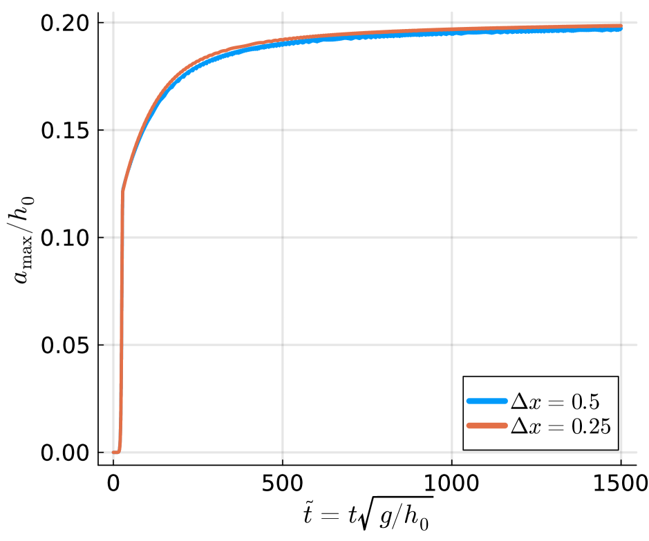
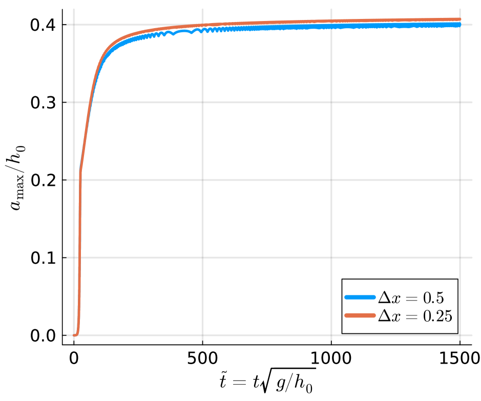
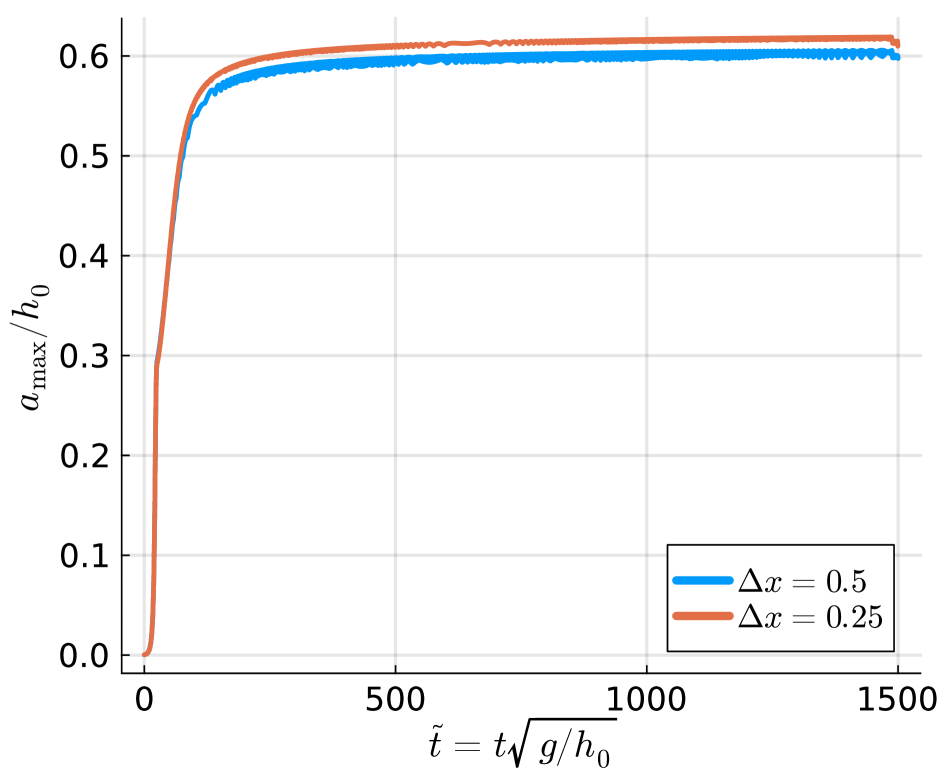
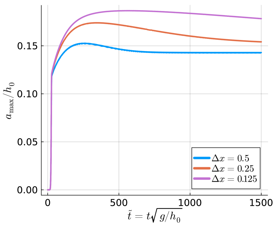
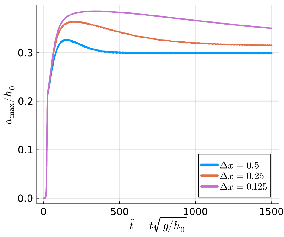
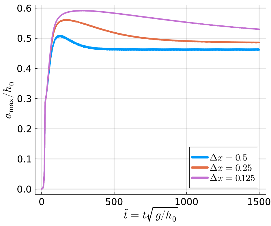
Figure 15: Favre waves. Evolution of the maximum amplitude obtained from the original SGN system with nonlinearities $\displaystyle\varepsilon=0.1$ (left), $\displaystyle\varepsilon=0.2$ (center), and $\displaystyle\varepsilon=0.3$ (right). Top: structure-preserving second-order finite difference scheme. Bottom: second-order finite difference with artificial viscosity.

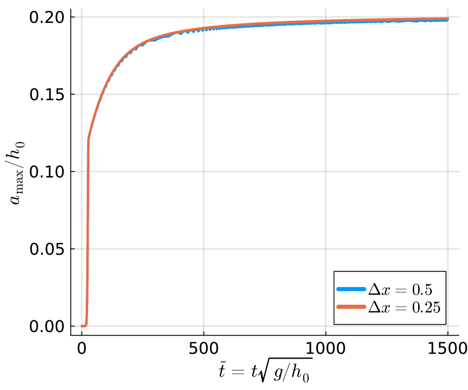
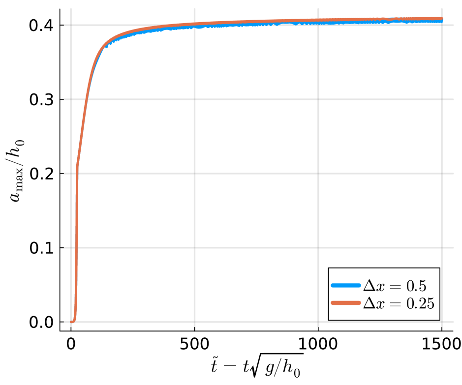
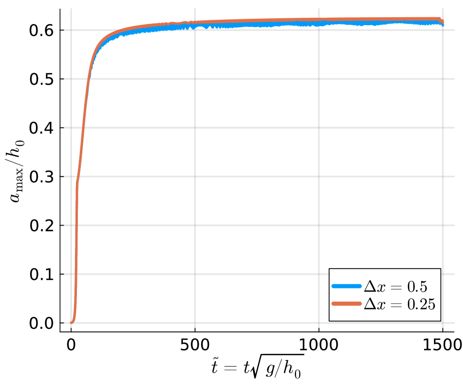
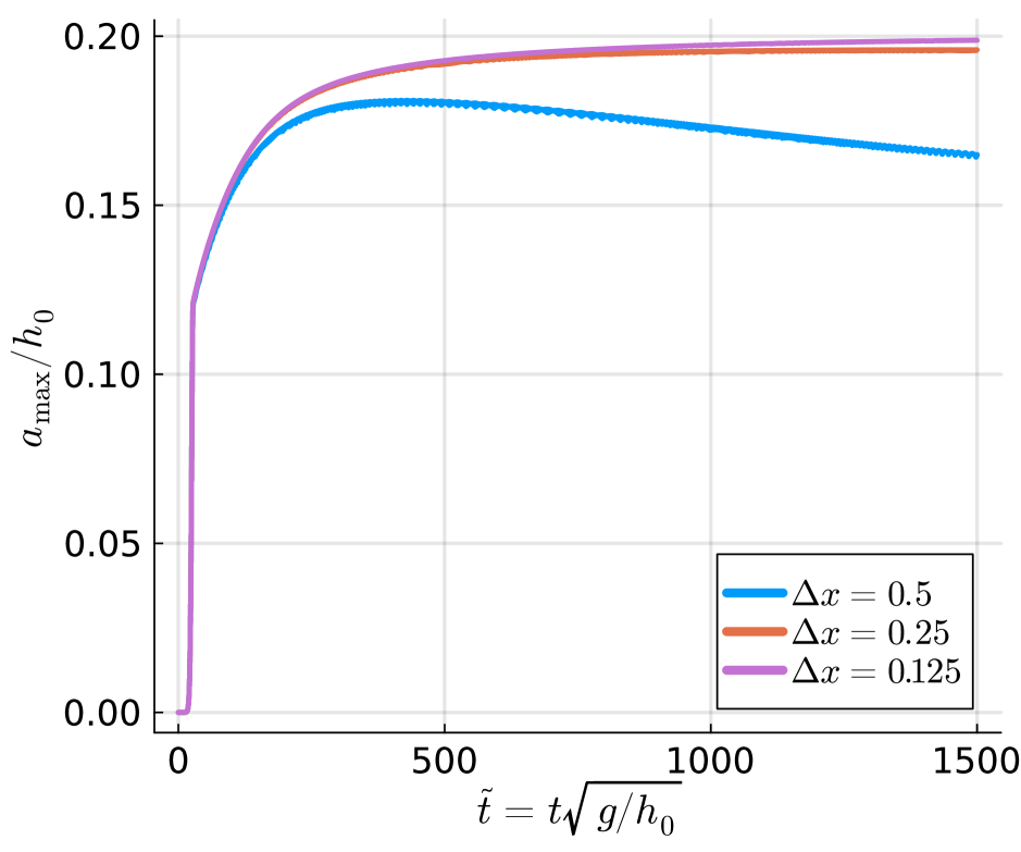
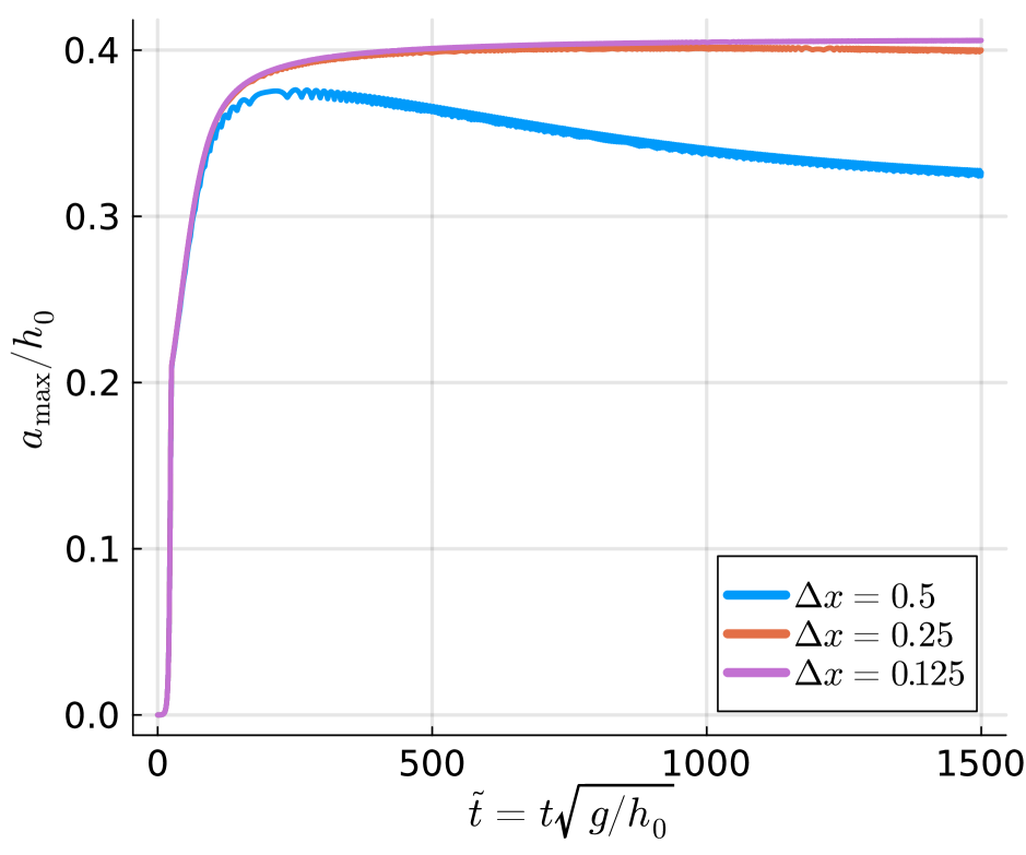
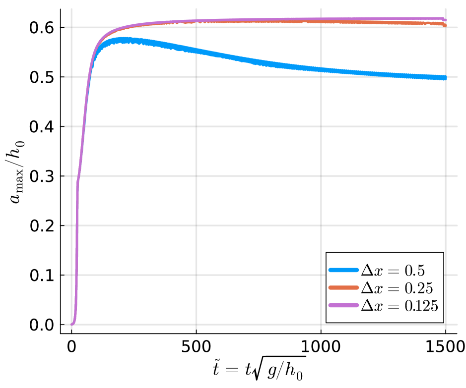
Figure 16: Favre waves. Evolution of the maximum amplitude obtained from the original SGN system with nonlinearities $\displaystyle\varepsilon=0.1$ (left), $\displaystyle\varepsilon=0.2$ (center), and $\displaystyle\varepsilon=0.3$ (right). Top: structure-preserving fourth-order finite difference scheme. Bottom: fourth-order finite difference with artificial viscosity.

These observations are confirmed by the plots of the maximum amplitude in Figures 15–16. The structure-preserving schemes provide already on the coarsest mesh an excellent approximation of the converged height. We can see that two more refinements would be required with a second-order scheme to match this value, while one refinement is required when using a fourth-order method. These results are qualitatively in line with those of [60]. They generalize such results to genuinely structure-preserving discretizations of the Serre-Green-Naghdi equations. We refer to the last reference for similar results when physical dissipation (friction) is included.

We do not show the wave lengths $\displaystyle\lambda$ of the Favre waves, since they increase over time (in the absence of friction/dissipation). This is in accordance with the results we have observed for the soliton fission problem in Section 11.7. However, we compare for completeness the numerical maximal amplitudes $\displaystyle a_{\mathrm{max}}$ with the data by [36, 128]. To this end, we compute $\displaystyle a_{\mathrm{max}}$ for different Froude numbers

$$\mathrm{Fr}=\frac{\sigma}{\sqrt{gh_{0}}}=\sqrt{(1+\varepsilon)(1+\varepsilon/2)}$$

by choosing $\displaystyle\varepsilon\in\{0.02,0.06,0.10,\dots,0.30\}$ for $\displaystyle\Delta x=0.02$, where $\displaystyle\sigma$ is the non-dispersive/average bore speed. We stop the simulations when the first wave (with amplitude $\displaystyle a_{\mathrm{max}}$) has travelled roughly the same distance as in the experiments, i.e., $\displaystyle 63.5\text{\,}\mathrm{m}$. The results are shown in Figure 17. The numerical and experimental data agree very well for Froude numbers $\displaystyle\mathrm{Fr}<1.25$. For larger Froude numbers, wave breaking modelling is required to capture the correct amplitudes.

(a) Hyperbolic approximation with $\displaystyle\lambda=500$.

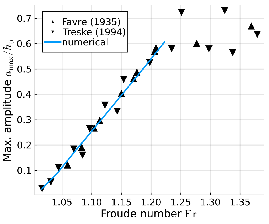
(b) Serre-Green-Naghdi equations.

Figure 17: Favre waves: maximal amplitude $\displaystyle a_{\mathrm{max}}$ against Froude number $\displaystyle\mathrm{Fr}=\sigma/\sqrt{gh_{0}}$. Comparison with experimental data of Favre [36] and Treske [128]. Numerical results with fourth-order structure-preserving finite differences with central operators for the hyperbolic approximation and upwind operators for the original Serre-Green-Naghdi equations.

11.9 Dingemans experiment

In this section, we compare numerical results obtained with our new energy-conserving methods with experimental data from [24, 25]. This setup is similar to classical test cases such as [4] that have been used to validate numerical models for water waves, e.g., [79, 65].

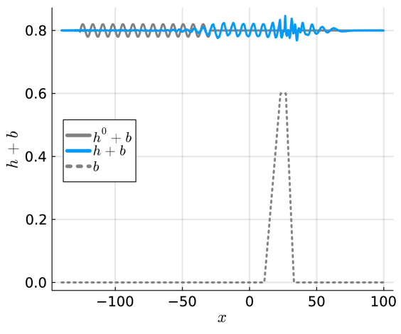
Figure 18: Initial setup and numerical solution at time $\displaystyle t=40$ obtained with fourth-order accurate upwind finite difference methods with $\displaystyle\Delta x=0.24$ applied to the mild-slope approximation of the Serre-Green-Naghdi equations for the Dingemans experiment.

The initial setup as well as a numerical solution of the mild-slope approximation are shown in Figure 18. The original experiment of Dingemans [24, 25] used a wave maker at $\displaystyle x=0$ to produce water waves with an initial amplitude of $\displaystyle A=0.02$ moving to the right. For the numerical simulations, choose the spatial domain $\displaystyle[-140,100]$ and initialize the numerical solution with a sinusoidal perturbation of the still water height $\displaystyle h=0.8$ with amplitude $\displaystyle A=0.02$. The phase of the perturbations and the corresponding velocity perturbation are chosen based on the dispersion relation of the Euler equations as in [122, 70]. The offset of the perturbation is chosen manually such that the phase at the first wave gauge matches the experimental data reasonably well.

The bottom is flat except a trapezoidal bar starting at $\displaystyle x=11.01$. Between $\displaystyle x=11.01$ and $\displaystyle x=23.04$, the bottom increases linearly from $\displaystyle b=0$ to $\displaystyle b=0.6$. The bottom has a small plateau between $\displaystyle x=23.04$ and $\displaystyle x=27.04$ with $\displaystyle b=0.6$ and decreases linearly from $\displaystyle b=0.6$ to $\displaystyle b=0$ between $\displaystyle x=27.04$ and $\displaystyle x=33.07$.

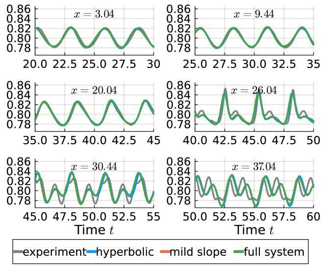
Figure 19: Experimental data of [24, 25] and total water height $\displaystyle h+b$ of the numerical solutions at the wave gauges over time obtained with fourth-order accurate finite difference methods with $\displaystyle\Delta x=0.24$. The hyperbolic approximation uses $\displaystyle\lambda=500$.

The values of the numerical solutions are compared to the experimental data at six wave gauges in Figure 19. First, we observe that the numerical solutions agree very well with each other — the results obtained using the hyperbolic approximation and the original SGN equations with/without mild-slope approximation are nearly indistinguishable. Moreover, the numerical results agree very well with the experimental data at the first three wave gauges. The agreement is less good but still qualitatively correct at the remaining wave gauges above and to the right of the plateau of the trapezoidal bar. This is within the limitations of the model used in terms of dispersion relation [116, 40]. However, the amplitudes of the numerical solutions are still in agreement with the experiments.

11.10 Preliminary comparison of runtime efficiency

The relative computational costs of discretizations of the hyperbolic approximation and the original SGN equations depend strongly on the parameter $\displaystyle\lambda$. For most numerical results presented above, we have chosen $\displaystyle\lambda=500$ as a compromise between accuracy and computational costs since the numerical solutions obtained with the hyperbolic approximation and this value of the parameter $\displaystyle\lambda$ are visually (nearly) indistinguishable from the results obtained with the original SGN equations. The only exception is the Riemann problem in Section 11.6, where a value of $\displaystyle\lambda=1000$ is required to obtain visually indistinguishable results.

Table 5: Benchmarks of the total runtime of the numerical solutions obtained with the hyperbolic approximation and the original Serre-Green-Naghdi equations using finite differences with $\displaystyle N$ nodes.

(a) Setup of the conservation tests with variable bathymetry and second-order central operators (Sections 11.2 and 11.3).

	hyperbolic	hyperbolic	original	original
$\displaystyle N$	($\displaystyle\lambda=500$)	($\displaystyle\lambda=1000$)	(mild slope)	(full system)
1000	$\displaystyle 73.0\pm 21.0\text{\,}\mathrm{m}\mathrm{s}$	$\displaystyle 94.0\pm 3.3\text{\,}\mathrm{m}\mathrm{s}$	$\displaystyle 178.3\pm 2.3\text{\,}\mathrm{m}\mathrm{s}$	$\displaystyle 189.7\pm 4.2\text{\,}\mathrm{m}\mathrm{s}$
2000	$\displaystyle 234.0\pm 38.0\text{\,}\mathrm{m}\mathrm{s}$	$\displaystyle 301.1\pm 7.2\text{\,}\mathrm{m}\mathrm{s}$	$\displaystyle 359.1\pm 8.5\text{\,}\mathrm{m}\mathrm{s}$	$\displaystyle 378.0\pm 11.0\text{\,}\mathrm{m}\mathrm{s}$
3000	$\displaystyle 441.4\pm 4.9\text{\,}\mathrm{m}\mathrm{s}$	$\displaystyle 611.0\pm 18.0\text{\,}\mathrm{m}\mathrm{s}$	$\displaystyle 536.2\pm 7.4\text{\,}\mathrm{m}\mathrm{s}$	$\displaystyle 581.0\pm 29.0\text{\,}\mathrm{m}\mathrm{s}$
4000	$\displaystyle 776.8\pm 5.1\text{\,}\mathrm{m}\mathrm{s}$	$\displaystyle 1.089\pm 0.048\text{\,}\mathrm{s}$	$\displaystyle 724.4\pm 3.0\text{\,}\mathrm{m}\mathrm{s}$	$\displaystyle 781.0\pm 32.0\text{\,}\mathrm{m}\mathrm{s}$
5000	$\displaystyle 1.345\pm 0.031\text{\,}\mathrm{s}$	$\displaystyle 1.869\pm 0.051\text{\,}\mathrm{s}$	$\displaystyle 967.0\pm 27.0\text{\,}\mathrm{m}\mathrm{s}$	$\displaystyle 941.0\pm 20.0\text{\,}\mathrm{m}\mathrm{s}$

(b) Setup of the Favre waves with $\displaystyle\varepsilon=0.2$ and fourth-order central/upwind operators for the hyperbolic/original equations (Section 11.8).

	hyperbolic	hyperbolic	original	original	original
$\displaystyle N$	($\displaystyle\lambda=500$)	($\displaystyle\lambda=1000$)	(flat bottom)	(mild slope)	(full system)
1000	$\displaystyle 68.3\pm 2.5\text{\,}\mathrm{m}\mathrm{s}$	$\displaystyle 96.6\pm 5.2\text{\,}\mathrm{m}\mathrm{s}$	$\displaystyle 132.8\pm 4.1\text{\,}\mathrm{m}\mathrm{s}$	$\displaystyle 163.5\pm 6.1\text{\,}\mathrm{m}\mathrm{s}$	$\displaystyle 162.3\pm 1.9\text{\,}\mathrm{m}\mathrm{s}$
2000	$\displaystyle 236.0\pm 11.0\text{\,}\mathrm{m}\mathrm{s}$	$\displaystyle 339.0\pm 23.0\text{\,}\mathrm{m}\mathrm{s}$	$\displaystyle 300.1\pm 4.3\text{\,}\mathrm{m}\mathrm{s}$	$\displaystyle 358.5\pm 6.6\text{\,}\mathrm{m}\mathrm{s}$	$\displaystyle 382.0\pm 12.0\text{\,}\mathrm{m}\mathrm{s}$
3000	$\displaystyle 517.0\pm 40.0\text{\,}\mathrm{m}\mathrm{s}$	$\displaystyle 741.3\pm 3.9\text{\,}\mathrm{m}\mathrm{s}$	$\displaystyle 517.6\pm 5.8\text{\,}\mathrm{m}\mathrm{s}$	$\displaystyle 667.5\pm 4.8\text{\,}\mathrm{m}\mathrm{s}$	$\displaystyle 664.0\pm 13.0\text{\,}\mathrm{m}\mathrm{s}$
4000	$\displaystyle 1.1796\pm 0.0073\text{\,}\mathrm{s}$	$\displaystyle 1.895\pm 0.014\text{\,}\mathrm{s}$	$\displaystyle 753.0\pm 10.0\text{\,}\mathrm{m}\mathrm{s}$	$\displaystyle 964.0\pm 12.0\text{\,}\mathrm{m}\mathrm{s}$	$\displaystyle 971.4\pm 8.3\text{\,}\mathrm{m}\mathrm{s}$
5000	$\displaystyle 2.0021\pm 0.006\text{\,}\mathrm{s}$	$\displaystyle 3.128\pm 0.025\text{\,}\mathrm{s}$	$\displaystyle 1.109\pm 0.003\text{\,}\mathrm{s}$	$\displaystyle 1.338\pm 0.009\text{\,}\mathrm{s}$	$\displaystyle 1.368\pm 0.012\text{\,}\mathrm{s}$

To give a first impression of the computational costs of the methods, we benchmark the total runtime (wallclock time) required to compute the numerical solutions from Sections 11.2 and 11.8 on a single core of a MacBook (M2 chip) using the Julia package BenchmarkTools.jl [18]. The results are reported in Table 5. While we do not aim to present a detailed performance study including the effects of various constraints and effects, the results show that there is no significant difference between the two versions of the original Serre-Green-Naghdi equations with variable bathymetry. Moreover, the computational costs of the hyperbolic approximation appear to increase faster with the number of grid nodes than the costs of the original system. In particular, the hyperbolic approximation with $\displaystyle\lambda=500$ is faster than the original system (by a factor of roughly three) for $\displaystyle N=1000$ nodes. For $\displaystyle N\in\{2000,3000\}$, the runtimes of the hyperbolic approximation with $\displaystyle\lambda=500$ are still smaller than the runtimes of the original systems. This changes around $\displaystyle N=4000$ nodes; for $\displaystyle N=5000$ nodes, the original systems are faster than the hyperbolic approximation.

However, these performance benchmarks are done with the research code we have implemented for this article. This code is not optimized for performance. While we expect that the efficiency of the hyperbolic version should be reasonably good, the elliptic solves required for the original system are likely to be suboptimal. In particular, most of the total runtime is spent assembling (multiplying sparse/diagonal matrices) and solving (Cholesky factorization of SuiteSparse) the elliptic problems.

12 Summary and conclusions

We have developed structure-preserving numerical methods for the Serre-Green-Naghdi equations in their original formulation and the first-order hyperbolic approximation of [37, 13]. Starting with the hyperbolic approximation for flat bathymetry in Section 5, we have derived the methods for models with increasing complexity, including variable bathymetry for the hyperbolic approximation (Section 7) and the original Serre-Green-Naghdi equations (Sections 8 and 9). All methods conserve the total water mass, the total energy, and are well-balanced with respect to the lake-at-rest steady state. Moreover, the numerical methods discretizing the original Serre-Green-Naghdi equations conserve the total momentum for flat bathymetry.

We have demonstrated the suitability of the novel structure-preserving numerical methods in a range of numerical experiments, including academic test cases such as convergence tests. We have also demonstrated the importance of energy-conserving methods for long-time simulations of solitary waves in Section 11.5, where energy conservation reduces the error growth in time from quadratic to linear. Even without exact preservation in time, we have also shown the impact of energy conservation in providing correct predictions of wave heights in long-time propagation. Moreover, we have shown that our numerical methods reproduce experimental data, e.g., for Favre waves (Section 11.8) and the flow over a trapezoidal bar (Section 11.9).

Preliminary performance benchmarks show that the hyperbolic approximation can be very efficient on coarse meshes. On finer meshes, the original formulations of the Serre-Green-Naghdi equations are more efficient (cf. Section 11.10).

Similar to Jouy et al. [60], we have found that structure-preserving numerical methods for the Serre-Green-Naghdi equations can efficiently capture the qualitatively correct behavior of water waves in a range of scenarios. Compared to methods including artificial dissipation/viscosity, the energy-preserving methods show the correct long-time behavior of the amplitude and shape of waves even on coarse meshes with low-order discretizations. This poses the question of the appropriateness of using entropy/energy dissipation as a stability criterion. Certainly, structure-preserving methods are a promising approach for the numerical simulation of water waves on coarse meshes (required in practice) and long-time simulations, typical of the operational context.

Our investigations can be extended in several directions. For example, we could check whether there are more energy-conservative split forms starting from the two-parameter family of energy-conservative split forms of the classical shallow water equations of [99]. Moreover, we could investigate the influence of possible other split forms of the non-hydrostatic pressure term of the Serre-Green-Naghdi equations, other upwind versions of the non-hydrostatic pressure term, and more general narrow-stencil second-derivative SBP operators instead of upwind operators, e.g., in Lemma 14. Further extensions include other boundary conditions, e.g., a reflective/wall boundary condition [87].

References

- [1] Rémi Abgrall, Jan Nordström, Philipp Öffner, and Svetlana Tokareva. Analysis of the SBP-SAT stabilization for finite element methods part I: Linear problems. Journal of Scientific Computing, 85(2):1–29, 2020.
- [2] Patrick R Amestoy, Timothy A Davis, and Iain S Duff. Algorithm 837: AMD, an approximate minimum degree ordering algorithm. ACM Transactions on Mathematical Software (TOMS), 30(3):381–388, 2004.
- [3] T. Baba, N. Chikasada, K. Imai, Y. Tanioka, and S. Kodaira. Frequency dispersion amplifies tsunamis caused by outer-rise normal faults. Sci.Rep., 1, 2021.
- [4] S Beji and J.A. Battjes. Experimental investigation of wave propagation over a bar. Coastal Engineering, 19(1–2):151–162, 1993.
- [5] Martin Berzins. Temporal error control for convection-dominated equations in two space dimensions. SIAM Journal on Scientific Computing, 16(3):558–580, 1995.
- [6] Jeff Bezanson, Alan Edelman, Stefan Karpinski, and Viral B Shah. Julia: A fresh approach to numerical computing. SIAM Review, 59(1):65–98, 2017.
- [7] Abhijit Biswas and David I Ketcheson. Accurate solution of the nonlinear Schrödinger equation via conservative multiple-relaxation ImEx methods, 2023.
- [8] Daria Bolbot, Dimitrios Mitsotakis, and Athanasios E. Tzavaras. Oscillatory and regularized shock waves for a modified Serre-Green-Naghdi system. Studies in Applied Mathematics, 153(1):e12694, 2024.
- [9] P. Bonneton, N. Bonneton, J.-P. Parisot, and B. Castelle. Tidal bore dynamics in funnel-shaped estuaries. Journal of Geophysical Research: Oceans, 120(2):923–941, 2015.
- [10] François Bouchut. Nonlinear Stability of Finite Volume Methods for Hyperbolic Conservation Laws and Well-Balanced Schemes for Sources. Birkhäuser Verlag, Basel, 2004.
- [11] D. Bresch and B. Desjardins. Sur un modèle de Saint-Venant visqueux et sa limite quasi-géostrophique. Comptes Rendus. Mathématique, 335(12):1079–1084, 2002.
- [12] Larkspur Brudvik-Lindner, Dimitrios Mitsotakis, and Athanasios E Tzavaras. Oscillatory and regularized shock waves for a dissipative Peregrine-Boussinesq system. IMA Journal of Applied Mathematics, 88(4):602–631, 10 2023.
- [13] S. Busto, M. Dumbser, C. Escalante, N. Favrie, and S. Gavrilyuk. On High Order ADER Discontinuous Galerkin Schemes for First Order Hyperbolic Reformulations of Nonlinear Dispersive Systems. Journal of Scientific Computing, 87, 2021.
- [14] Mark H Carpenter, Travis C Fisher, Eric J Nielsen, and Steven H Frankel. Entropy stable spectral collocation schemes for the Navier-Stokes equations: Discontinuous interfaces. SIAM Journal on Scientific Computing, 36(5):B835–B867, 2014.
- [15] A. Cauquis, M. Ricchiuto, and P. Heinrich. Lax–wendroff schemes with polynomial extrapolation and simplified lax–wendroff schemes for dispersive waves: A comparative study. Water Waves, 4:345–377, 2022.
- [16] Jesse Chan. On discretely entropy conservative and entropy stable discontinuous Galerkin methods. Journal of Computational Physics, 362:346–374, 2018.
- [17] R. Chassagne, A.G. Filippini, M. Ricchiuto, and P. Bonneton. Dispersive and dispersive-like bores in channels with sloping banks. Journal of mechanics, 870:595?616, 2019.
- [18] Jiahao Chen and Jarrett Revels. Robust benchmarking in noisy environments, 08 2016.
- [19] Yanqing Chen, Timothy A Davis, William W Hager, and Sivasankaran Rajamanickam. Algorithm 887: CHOLMOD, supernodal sparse Cholesky factorization and update/downdate. ACM Transactions on Mathematical Software (TOMS), 35(3):1–14, 2008.
- [20] Y.-K. Choi, F. Shi, M. Malej, J. M. Smith, J. T. Kirby, and S. T. Grilli. Block-structured, equal-workload, multi-grid-nesting interface for the Boussinesq wave model FUNWAVE-TVD (total variation diminishing). Geoscientific Model Development, 15(14):5441–5459, 2022.
- [21] Simon Christ, Daniel Schwabeneder, Christopher Rackauckas, Michael Krabbe Borregaard, and Thomas Breloff. Plots.jl — a user extendable plotting API for the Julia programming language. Journal of Open Research Software, 2023.
- [22] Timothy A Davis, John R Gilbert, Stefan I Larimore, and Esmond G Ng. Algorithm 836: COLAMD, a column approximate minimum degree ordering algorithm. ACM Transactions on Mathematical Software (TOMS), 30(3):377–380, 2004.
- [23] J De Frutos and Jesus Maria Sanz-Serna. Accuracy and conservation properties in numerical integration: the case of the Korteweg-de Vries equation. Numerische Mathematik, 75(4):421–445, 1997.
- [24] Maarten W. Dingemans. Comparison of computations with Boussinesq-like models and laboratory measurements. Technical Report H1684.12, Delft Hydraulics, 1994.
- [25] Maarten W. Dingemans. Water Wave Propagation Over Uneven Bottoms, volume 13. World Scientific, 1997.
- [26] Vaibhav Kumar Dixit and Christopher Rackauckas. Optimization.jl: A unified optimization package, March 2023.
- [27] Angel Durán and Jesus Maria Sanz-Serna. The numerical integration of relative equilibrium solutions. Geometric theory. Nonlinearity, 11(6):1547, 1998.
- [28] Angel Durán and Jesus Maria Sanz-Serna. The numerical integration of relative equilibrium solutions. The nonlinear Schrödinger equation. IMA Journal of Numerical Analysis, 20(2):235–261, 2000.
- [29] Arnaud Duran and Fabien Marche. A discontinuous galerkin method for a new class of Green–Naghdi equations on simplicial unstructured meshes. Applied Mathematical Modelling, 45:840–864, 2017.
- [30] G. A. El. Resolution of a shock in hyperbolic systems modified by weak dispersion. Chaos: An Interdisciplinary Journal of Nonlinear Science, 15(3):037103, 10 2005.
- [31] G.A. El, R.H.J. Grimshaw, and N. F. Smyth. Unsteady undular bores in fully nonlinear shallow-water theory. Phys. Fluids, 18:027104, 2006.
- [32] G.A. El and M.A. Hoefer. Dispersive shock waves and modulation theory. Physica D: Nonlinear Phenomena, 333:11–65, 2016. Dispersive Hydrodynamics.
- [33] G.A. El, V.V. Khodorovskii, and A.V. Tyurina. Undular bore transition in bi-directional conservative wave dynamics. Phys. D Nonlinear Phenom., 206:232?251, 2005.
- [34] C. Escalante and T.M. de Luna. A general non-hydrostatic hyperbolic formulation for Boussinesq dispersive shallow flows and its numerical approximation. J.Sci.Comput., 83(62), 2020.
- [35] Claes Eskilsson, SJ Sherwin, and Lars Bergdahl. An unstructured spectral/hp element model for enhanced Boussinesq-type equations. Coastal Engineering, 53(11):947–963, 2006.
- [36] H. Favre. Etude théorique et expérimentale des ondes de translation dans les canaux découverts. Dunod, 1935.
- [37] N Favrie and S Gavrilyuk. A rapid numerical method for solving Serre-Green-Naghdi equations describing long free surface gravity waves. Nonlinearity, 30(7):2718, 2017.
- [38] David C Del Rey Fernández, Jason E Hicken, and David W Zingg. Review of summation-by-parts operators with simultaneous approximation terms for the numerical solution of partial differential equations. Computers & Fluids, 95:171–196, 2014.
- [39] A.G. Filippini, L. Arpaia P. Bonneton, and M. Ricchiuto. Modeling analysis of tidal bore formation in convergent estuaries. European Journal of Mechanics - B/Fluids, 73:55–68, 2019. Breaking Waves.
- [40] Andrea Gilberto Filippini, Stevan Bellec, Mathieu Colin, and Mario Ricchiuto. On the nonlinear behaviour of Boussinesq type models: Amplitude-velocity vs amplitude-flux forms. Coastal Engineering, 99:109–123, 2015.
- [41] Andrea Gilberto Filippini, Maria Kazolea, and Mario Ricchiuto. A flexible genuinely nonlinear approach for nonlinear wave propagation, breaking and run-up. Journal of Computational Physics, 310:381–417, 2016.
- [42] Travis C Fisher and Mark H Carpenter. High-order entropy stable finite difference schemes for nonlinear conservation laws: Finite domains. Journal of Computational Physics, 252:518–557, 2013.
- [43] Travis C Fisher, Mark H Carpenter, Jan Nordström, Nail K Yamaleev, and Charles Swanson. Discretely conservative finite-difference formulations for nonlinear conservation laws in split form: Theory and boundary conditions. Journal of Computational Physics, 234:353–375, 2013.
- [44] Ulrik Skre Fjordholm, Siddhartha Mishra, and Eitan Tadmor. Well-balanced and energy stable schemes for the shallow water equations with discontinuous topography. Journal of Computational Physics, 230(14):5587–5609, 2011.
- [45] Matteo Frigo and Steven G Johnson. The design and implementation of FFTW3. Proceedings of the IEEE, 93(2):216–231, 2005.
- [46] Fuchang Gao and Lixing Han. Implementing the Nelder-Mead simplex algorithm with adaptive parameters. Computational Optimization and Applications, 51(1):259–277, 2012.
- [47] Gregor Josef Gassner. A skew-symmetric discontinuous Galerkin spectral element discretization and its relation to SBP-SAT finite difference methods. SIAM Journal on Scientific Computing, 35(3):A1233–A1253, 2013.
- [48] Gregor Josef Gassner, Andrew Ross Winters, and David A Kopriva. A well balanced and entropy conservative discontinuous Galerkin spectral element method for the shallow water equations. Applied Mathematics and Computation, 272:291–308, 2016.
- [49] S. Gavrilyuk, B. Nkonga, K.-M. Shyue, and L. Truskinovsky. Stationary shock-like transition fronts in dispersive systems. Nonlinearity, 33:5477–5509, 2020.
- [50] S. Gavrilyuk and K.-M. Shyue. 2D Serre-Green-Naghdi equations over topography: Elliptic operator inversion method. Journal of Hydraulic Engineering, 150(1):04023054, 2024.
- [51] Jean-Frédéric Gerbeau and Benoit Perthame. Derivation of viscous saint-venant system for laminar shallow water; numerical validation, 2001.
- [52] S. Glimsdal, G. K. Pedersen, C. B. Harbitz, and F. Løvholt. Dispersion of tsunamis: does it really matter? Natural Hazards and Earth System Sciences, 13(6):1507–1526, 2013.
- [53] A. E. Green and P. M. Naghdi. A derivation of equations for wave propa-gation in water of variable depth. J.Fluid Mech., 78, 1976.
- [54] Jean-Luc Guermond, Chris Kees, Bojan Popov, and Eric Tovar. Hyperbolic relaxation technique for solving the dispersive Serre-Green-Naghdi equations with topography. Journal of Computational Physics, 450:110809, 2022.
- [55] Jean-Luc Guermond, Richard Pasquetti, and Bojan Popov. Entropy viscosity method for nonlinear conservation laws. Journal of Computational Physics, 230(11):4248–4267, 2011. Special issue High Order Methods for CFD Problems.
- [56] Jason E Hicken. Entropy-stable, high-order summation-by-parts discretizations without interface penalties. Journal of Scientific Computing, 82(2):50, 2020.
- [57] Jason E Hicken, David C Del Rey Fernández, and David W Zingg. Multidimensional summation-by-parts operators: General theory and application to simplex elements. SIAM Journal on Scientific Computing, 38(4):A1935–A1958, 2016.
- [58] M.A. Hoefer. Shock Waves in Dispersive Eulerian Fluids. J.Nonlinear Sci., 24:525–577, 2014.
- [59] H. T. Huynh. A flux reconstruction approach to high-order schemes including discontinuous Galerkin methods. In 18th AIAA Computational Fluid Dynamics Conference. American Institute of Aeronautics and Astronautics, 2007.
- [60] B. Jouy, D. Violeau, M. Ricchiuto, and M. Le. One dimensional modelling of favre waves in channels. Applied Mathematical Modelling, 133:170–194, 2024.
- [61] Ansgar Jüngel and Stefan Schuchnigg. Entropy-dissipating semi-discrete Runge-Kutta schemes for nonlinear diffusion equations. Communications in Mathematical Sciences, 15(1):27–53, 2017.
- [62] M Kazolea, AI Delis, IK Nikolos, and CE Synolakis. An unstructured finite volume numerical scheme for extended 2D Boussinesq-type equations. Coastal Engineering, 69:42–66, 2012.
- [63] M. Kazolea, A.G. Filippini, and M. Ricchiuto. Low dispersion finite volume/element discretization of the enhanced Green–Naghdi equations for wave propagation, breaking and runup on unstructured meshes. Ocean Modelling, 182:102157, 2023.
- [64] Maria Kazolea and Mario Ricchiuto. Full nonlinearity in weakly dispersive Boussinesq models: Luxury or necessity. Journal of Hydraulic Engineering, 150(1):04023061, 2024.
- [65] Maria Kazolea and Mario Ricchiuto. Full nonlinearity in weakly dispersive Boussinesq models: Luxury or necessity. Journal of Hydraulic Engineering, 150(1):04023061, 2024.
- [66] David I Ketcheson. Relaxation Runge-Kutta methods: Conservation and stability for inner-product norms. SIAM Journal on Numerical Analysis, 57(6):2850–2870, 2019.
- [67] David I Ketcheson, Mikael Mortensen, Matteo Parsani, and Nathanael Schilling. More efficient time integration for Fourier pseudo-spectral DNS of incompressible turbulence. International Journal for Numerical Methods in Fluids, 92(2):79–93, 2020.
- [68] James T. Kirby. Boussinesq models and their application to coastal processes across a wide range of scales. Journal of Waterway, Port, Coastal, and Ocean Engineering, 142(6):03116005, 2016.
- [69] Heinz-Otto Kreiss and Godela Scherer. Finite element and finite difference methods for hyperbolic partial differential equations. In Carl de Boor, editor, Mathematical Aspects of Finite Elements in Partial Differential Equations, pages 195–212, New York, 1974. Academic Press.
- [70] Joshua Lampert and Hendrik Ranocha. Structure-preserving numerical methods for two nonlinear systems of dispersive wave equations, 02 2024.
- [71] D Lannes. Modeling shallow water waves. Nonlinearity, 33(5):R1, mar 2020.
- [72] David Lannes and Fabien Marche. A new class of fully nonlinear and weakly dispersive Green–Naghdi models for efficient 2D simulations. Journal of Computational Physics, 282:238–268, 2015.
- [73] Marine Le Gal, Damien Violeau, and Michel Benoit. Influence of timescales on the generation of seismic tsunamis. European Journal of Mechanics - B/Fluids, 65:257–273, 2017.
- [74] Maojun Li, Liwei Xu, and Yongping Cheng. A CDG-FE method for the two-dimensional Green-Naghdi model with the enhanced dispersive property. Journal of Computational Physics, 399:108953, 2019.
- [75] Yi A Li. Hamiltonian structure and linear stability of solitary waves of the Green-Naghdi equations. Journal of Nonlinear Mathematical Physics, 9(Suppl 1):99–105, 2002.
- [76] Carlos Lozano. Entropy production by explicit Runge-Kutta schemes. Journal of Scientific Computing, 76(1):521–565, 2018.
- [77] Yvon Maday, Sidi M. Ould Kaber, and Eitan Tadmor. Legendre pseudospectral viscosity method for nonlinear conservation laws. SIAM Journal on Numerical Analysis, 30(2):321–342, 1993.
- [78] P. A. Madsen and H. A. Schaffer. Higher-order Boussinesq-type equations for surface gravity waves: derivation and analysis. Philosophical Transactions of the Royal Society of London. Series A: Mathematical, Physical and Engineering Sciences, 356(1749):3123–3181, 1998.
- [79] PA Madsen, B Banijamali, HA Schäffer, and OR Sørensen. Boussinesq type equations with high accuracy in dispersion and nonlinearity. In Coastal Engineering 1996, pages 95–108. 1996.
- [80] Ken Mattsson. Summation by parts operators for finite difference approximations of second-derivatives with variable coefficients. Journal of Scientific Computing, 51(3):650–682, 2012.
- [81] Ken Mattsson. Diagonal-norm upwind SBP operators. Journal of Computational Physics, 335:283–310, 2017.
- [82] Ken Mattsson and Jan Nordström. Summation by parts operators for finite difference approximations of second derivatives. Journal of Computational Physics, 199(2):503–540, 2004.
- [83] Alireza Mazaheri, Mario Ricchiuto, and Hiroaki Nishikawa. A first-order hyperbolic system approach for dispersion. Journal of Computational Physics, 321:593–605, 2016.
- [84] Dimitrios Mitsotakis, Hendrik Ranocha, David I Ketcheson, and Endre Süli. A conservative fully-discrete numerical method for the regularized shallow water wave equations. SIAM Journal on Scientific Computing, 42, 04 2021.
- [85] Patrick Kofod Mogensen and Asbjørn Nilsen Riseth. Optim: A mathematical optimization package for Julia. Journal of Open Source Software, 3(24):615, 2018.
- [86] John A Nelder and Roger Mead. A simplex method for function minimization. The computer journal, 7(4):308–313, 1965.
- [87] Sebastian Noelle, Martin Parisot, and Tabea Tscherpel. A class of boundary conditions for time-discrete Green-Naghdi equations with bathymetry. SIAM Journal on Numerical Analysis, 60(5):2681–2712, 2022.
- [88] Jan Nordström and Martin Björck. Finite volume approximations and strict stability for hyperbolic problems. Applied Numerical Mathematics, 38(3):237–255, 2001.
- [89] Jan Nordström, Karl Forsberg, Carl Adamsson, and Peter Eliasson. Finite volume methods, unstructured meshes and strict stability for hyperbolic problems. Applied Numerical Mathematics, 45(4):453–473, 2003.
- [90] Philipp Öffner, Jan Glaubitz, and Hendrik Ranocha. Analysis of artificial dissipation of explicit and implicit time-integration methods. International Journal of Numerical Analysis and Modeling, 17(3):332–349, 05 2020.
- [91] Ivo FD Oliveira and Ricardo HC Takahashi. An enhancement of the bisection method average performance preserving minmax optimality. ACM Transactions on Mathematical Software (TOMS), 47(1):1–24, 2020.
- [92] Sigrun Ortleb. On the stability of IMEX upwind gSBP schemes for linear advection-diffusion equations, 2023.
- [93] Avik Pal, Flemming Holtorf, Axel Larsson, Torkel Loman, Utkarsh, Frank Schäfer, Qingyu Qu, Alan Edelman, and Chris Rackauckas. NonlinearSolve.jl: High-performance and robust solvers for systems of nonlinear equations in Julia. 2024.
- [94] Nishant Panda, Clint Dawson, Yao Zhang, Andrew B. Kennedy, Joannes J. Westerink, and Aaron S. Donahue. Discontinuous Galerkin methods for solving Boussinesq–Green–Naghdi equations in resolving non-linear and dispersive surface water waves. Journal of Computational Physics, 273:572–588, 2014.
- [95] M. Parisot. Entropy-satisfying scheme for a hierarchy of dispersive reduced models of free surface flow. International Journal for Numerical Methods in Fluids, 91(10):509–531, 2019.
- [96] Richard Pasquetti. Viscous stabilizations for high order approximations of Saint-Venant and Boussinesq flows. In Marco L. Bittencourt, Ney A. Dumont, and Jan S. Hesthaven, editors, Spectral and High Order Methods for Partial Differential Equations ICOSAHOM 2016, pages 519–531, Cham, 2017. Springer International Publishing.
- [97] JPA Pitt, Christopher Zoppou, and SG Roberts. Behaviour of the Serre equations in the presence of steep gradients revisited. Wave Motion, 76:61–77, 2018.
- [98] Christopher Rackauckas and Qing Nie. DifferentialEquations.jl – A performant and feature-rich ecosystem for solving differential equations in Julia. Journal of Open Research Software, 5(1):15, 2017.
- [99] Hendrik Ranocha. Shallow water equations: Split-form, entropy stable, well-balanced, and positivity preserving numerical methods. GEM – International Journal on Geomathematics, 8(1):85–133, 04 2017.
- [100] Hendrik Ranocha. Mimetic properties of difference operators: Product and chain rules as for functions of bounded variation and entropy stability of second derivatives. BIT Numerical Mathematics, 59(2):547–563, 06 2019.
- [101] Hendrik Ranocha. On strong stability of explicit Runge-Kutta methods for nonlinear semibounded operators. IMA Journal of Numerical Analysis, 41(1):654–682, 01 2021.
- [102] Hendrik Ranocha. SummationByPartsOperators.jl: A Julia library of provably stable semidiscretization techniques with mimetic properties. Journal of Open Source Software, 6(64):3454, 08 2021.
- [103] Hendrik Ranocha, Lisandro Dalcin, and Matteo Parsani. Fully-discrete explicit locally entropy-stable schemes for the compressible Euler and Navier-Stokes equations. Computers and Mathematics with Applications, 80(5):1343–1359, 07 2020.
- [104] Hendrik Ranocha, Lisandro Dalcin, Matteo Parsani, and David I. Ketcheson. Optimized Runge-Kutta methods with automatic step size control for compressible computational fluid dynamics. Communications on Applied Mathematics and Computation, 4:1191–1228, 11 2021.
- [105] Hendrik Ranocha and David I Ketcheson. Energy stability of explicit Runge-Kutta methods for nonautonomous or nonlinear problems. SIAM Journal on Numerical Analysis, 58(6):3382–3405, 11 2020.
- [106] Hendrik Ranocha and David I Ketcheson. Relaxation Runge-Kutta methods for Hamiltonian problems. Journal of Scientific Computing, 84(1), 07 2020.
- [107] Hendrik Ranocha, Lajos Lóczi, and David I Ketcheson. General relaxation methods for initial-value problems with application to multistep schemes. Numerische Mathematik, 146:875–906, 10 2020.
- [108] Hendrik Ranocha, Dimitrios Mitsotakis, and David I Ketcheson. A broad class of conservative numerical methods for dispersive wave equations. Communications in Computational Physics, 29(4):979–1029, 02 2021.
- [109] Hendrik Ranocha and Philipp Öffner. stability of explicit Runge-Kutta schemes. Journal of Scientific Computing, 75(2):1040–1056, 05 2018.
- [110] Hendrik Ranocha, Philipp Öffner, and Thomas Sonar. Summation-by-parts operators for correction procedure via reconstruction. Journal of Computational Physics, 311:299–328, 04 2016.
- [111] Hendrik Ranocha, Manuel Quezada de Luna, and David I Ketcheson. On the rate of error growth in time for numerical solutions of nonlinear dispersive wave equations. Partial Differential Equations and Applications, 2(6):76, 10 2021.
- [112] Hendrik Ranocha and Mario Ricchiuto. Reproducibility repository for ”Structure-preserving approximations of the Serre-Green-Naghdi equations in standard and hyperbolic form”. https://github.com/ranocha/2024_serre_green_naghdi, 2024.
- [113] Hendrik Ranocha, Mohammed Sayyari, Lisandro Dalcin, Matteo Parsani, and David I. Ketcheson. Relaxation Runge–Kutta methods: Fully discrete explicit entropy-stable schemes for the compressible Euler and Navier–Stokes equations. SIAM Journal on Scientific Computing, 42(2):A612–A638, 2020.
- [114] Hendrik Ranocha, Mohammed Sayyari, Lisandro Dalcin, Matteo Parsani, and David I. Ketcheson. Relaxation Runge-Kutta methods: Fully-discrete explicit entropy-stable schemes for the compressible Euler and Navier-Stokes equations. SIAM Journal on Scientific Computing, 42(2):A612–A638, 03 2020.
- [115] Hendrik Ranocha, Andrew R Winters, Hugo Guillermo Castro, Lisandro Dalcin, Michael Schlottke-Lakemper, Gregor J Gassner, and Matteo Parsani. On error-based step size control for discontinuous Galerkin methods for compressible fluid dynamics. Communications on Applied Mathematics and Computation, 05 2023.
- [116] M. Ricchiuto and A.G. Filippini. Upwind residual discretization of enhanced Boussinesq equations for wave propagation over complex bathymerties. J. Comput. Phys., 271:306–341, 2014.
- [117] Robert D Richtmyer and Keith William Morton. Difference Methods for Boundary-Value Problems. John Wiley & Sons, New York, London, Sydney, 1967.
- [118] Jesus Maria Sanz-Serna. An explicit finite-difference scheme with exact conservation properties. Journal of Computational Physics, 47(2):199–210, 1982.
- [119] F. Serre. Contribution â l’étude des écoulements permanents et variables dans les canaux. Houille Blanche, 8, 1953.
- [120] Bo Strand. Summation by parts for finite difference approximations for . Journal of Computational Physics, 110(1):47–67, 1994.
- [121] Zheng Sun and Chi-Wang Shu. Strong stability of explicit Runge-Kutta time discretizations. SIAM Journal on Numerical Analysis, 57(3):1158–1182, 2019.
- [122] Magnus Svärd and Henrik Kalisch. A novel energy-bounded Boussinesq model and a well balanced and stable numerical discretisation, 2023.
- [123] Magnus Svärd and Jan Nordström. Review of summation-by-parts schemes for initial-boundary-value problems. Journal of Computational Physics, 268:17–38, 2014.
- [124] Eitan Tadmor. Convergence of spectral methods for nonlinear conservation laws. SIAM Journal on Numerical Analysis, 26(1):30–44, 1989.
- [125] Sasan Tavakkol and Patrick Lynett. Celeris base: An interactive and immersive Boussinesq-type nearshore wave simulation software. Computer Physics Communications, 248:106966, 2020.
- [126] Sergey Tkachenko, Sergey Gavrilyuk, and Jacques Massoni. Extended Lagrangian approach for the numerical study of multidimensional dispersive waves: Applications to the Serre-Green-Naghdi equations. Journal of Computational Physics, 477:111901, 2023.
- [127] Davide Torlo and Mario Ricchiuto. Model order reduction strategies for weakly dispersive waves. Mathematics and Computers in Simulation, 205:997–1028, 2023.
- [128] A. Treske. Undular bores (Favre-waves) in open channels - Experimental studies. Journal of Hydraulic Research, 32(3):355–370, May 1994.
- [129] Ch Tsitouras. Runge-Kutta pairs of order 5 (4) satisfying only the first column simplifying assumption. Computers & Mathematics with Applications, 62(2):770–775, 2011.
- [130] Maciej Waruszewski, Jeremy E Kozdon, Lucas C Wilcox, Thomas H Gibson, and Francis X Giraldo. Entropy stable discontinuous Galerkin methods for balance laws in non-conservative form: Applications to the Euler equations with gravity. Journal of Computational Physics, 468:111507, 2022.
- [131] Ge Wei, James T Kirby, Stephan T Grilli, and Ravishankar Subramanya. A fully nonlinear Boussinesq model for surface waves. Part 1. Highly nonlinear unsteady waves. Journal of Fluid Mechanics, 294:71–92, 1995.
- [132] Niklas Wintermeyer, Andrew Ross Winters, Gregor Josef Gassner, and David A Kopriva. An entropy stable nodal discontinuous Galerkin method for the two dimensional shallow water equations on unstructured curvilinear meshes with discontinuous bathymetry. Journal of Computational Physics, 340:200–242, 2017.
- [133] Ge Yan, Sharanjeet Kaur, Jason E Hicken, and Jeffrey W Banks. Entropy-stable Galerkin difference discretization on unstructured grids. In AIAA AVIATION 2020 FORUM, page 3033, 2020.
- [134] Ye Yuan, Fengyan Shi, James T. Kirby, and Fujiang Yu. FUNWAVE-GPU: Multiple-GPU acceleration of a Boussinesq-type wave model. Journal of Advances in Modeling Earth Systems, 12(5):e2019MS001957, 2020. e2019MS001957 10.1029/2019MS001957.
- [135] Hong Zhang, Xu Qian, Jingye Yan, and Songhe Song. Highly efficient invariant-conserving explicit Runge-Kutta schemes for nonlinear hamiltonian differential equations. Journal of Computational Physics, page 109598, 2020.