Applications of Scientific Machine Learning for the Analysis of Functionally Graded Porous Beams

Abstract

This study investigates different Scientific Machine Learning (SciML) approaches for the analysis of functionally graded (FG) porous beams and compares them under a new framework. The beam material properties are assumed to vary as an arbitrary continuous function. The methods consider the output of a neural network/operator as an approximation to the displacement fields and derive the equations governing beam behavior based on the continuum formulation. The methods are implemented in the framework and formulated by three approaches: (a) the vector approach leads to a Physics-Informed Neural Network (PINN), (b) the energy approach brings about the Deep Energy Method (DEM), and (c) the data-driven approach, which results in a class of Neural Operator methods. Finally, a neural operator has been trained to predict the response of the porous beam with functionally graded material under any porosity distribution pattern and any arbitrary traction condition. The results are validated with analytical and numerical reference solutions. The data and code accompanying this manuscript will be publicly available at https://github.com/eshaghi-ms/DeepNetBeam.

Keywords— Functionally graded material, Porous beam, Physics-informed neural network, Deep energy methods, Fourier Neural Operator, Scientific Machine Learning

1 Introduction

In the field of engineering, exploring novel materials with customized qualities has led to the emergence of Functionally Graded Materials (FGMs) which represent a class of composite materials characterized by gradual variations in material properties, resulting in unique characteristics that are not possible with homogeneous materials [1]. This continuous variation offers a range of advantages over homogeneous materials, including the ability to customize properties such as mechanical, thermal, electrical, and magnetic characteristics. Moreover, this refinement reduces thermal stress through gradual variation of thermal expansion coefficients, thereby minimizing the risk of thermal cracking [2]. FGMs also provide thermal protection and corrosion resistance, making them valuable in the aerospace, automotive, and energy industries. Their lightweight design, combined with structural integrity, allows the creation of structures suitable for weight-sensitive applications [3].

On the other hand, due to the broad application of beams across diverse fields including civil engineering, marine, military, and aeronautics industries, it is imperative to investigate the mechanical response of beams under different materials and loading conditions. Addressing this demand, beam theories are used to simplify the analysis of complex structures and predict their behavior. The primary goals of various beam theories, such as Classical Beam Theory (CBT), First Order Shear Deformation Theory (FSDT), and Higher-Order Shear Deformation Theory (HSDT), are to reach a balance between precision and efficiency [4]. The fundamental differences between these theories stem from their methods of modeling beam behavior. CBT simplifies the analysis by assuming that the cross-section remains plane and perpendicular to the beam’s axis after deformation, neglecting shear deformations. FSDT considers shear deformation effects but assumes constant transverse shear strains across the beam’s thickness. In contrast, HSDT accounts for variable transverse shear strains, resulting in a more accurate shear deformation. Significant research has been carried out in this area [5, 6]. Therefore it is of interest to investigate the analysis of FGMs for beams. Numerous studies in the literature also explore the mechanical analysis of FG beams, as evidenced by references [7, 8, 9, 10, 11, 12].

While beam theories have their utility in specific scenarios, their effectiveness might be limited when compared to the flexibility, autonomy, and data-driven nature of Machine Learning (ML) approaches in computational mechanics [13, 14]. ML has the potential to revolutionize the field by offering more accurate solutions, particularly for complex and real-world problems [15, 16]. For instance, Ebrahimi and Ezzati [17] studied Young’s modulus estimation in functionalized graphene-reinforced nanocomposites using ML. Their findings recommend implementing these models for faster results in engineering applications. Additionally, the research by Ahmed et al. [18] applied ML models (ANN, XGBoost, SVM) to predict shear behavior in ultra-high performance concrete I-shaped beans, where XGBoost exhibited higher accuracy. It highlights the improved accuracy of ML models compared to conventional design methods. Taking advantage of Artificial Neural Networks (ANNs), Mojtabaei et al. [19] successfully predicted elastic critical buckling loads and modal decompositions in thin-walled structural elements, showing their ability to address complicated challenges.

ML finds a wide variety of applications due to its ability to learn patterns from data and then generate the expected output. One significant application of this approach can be found in solving Partial Differential Equations (PDEs) [20, 21, 22]. The potential of using deep learning methods to approximate solutions for PDEs was investigated by Beck et al. [23]. These methods provide new possibilities for solving PDEs in various fields, especially in complex system modeling. The readers can find the history of different ANN methods for solving differential equations in the book by Yadav et al. [24]. This ML application led to the development of the field of Scientific Machine Learning (SciML).

SciML is an interdisciplinary field that combines techniques from scientific computing, machine learning, and domain-specific sciences. Its main purpose is to develop algorithms that combine the knowledge of physical systems (e.g., differential equations, and conservation laws) and the power of ML [25]. In traditional scientific computing, researchers use mathematical models to study the behavior of systems. However, these models often depend on simplifications and assumptions that may not capture the complexity of real-world phenomena. On the other hand, ML approaches are suitable for learning patterns and making predictions from data but may lack interpretability and struggle with extrapolation outside of the data distribution. SciML bridges this gap by merging scientific knowledge into ML algorithms [26].

Another utilization of SciML is in addressing beam-related problems within the field of structural mechanics. Beam-related problems can benefit from SciML’s potential to improve their analysis, design, and performance evaluation across diverse loading scenarios [27]. Therefore, we aim to formulate a new framework, named DeepNetBeam (DNB), which uses SciML for analyzing FG beams. For this purpose, there are three possible approaches to consider: (a) the vector approach followed in continuum mechanics, which leads to Physics-Informed Neural Networks (PINN), (b) the energy approach based on the principle of minimum total potential energy, leading to Deep Energy methods (DEM), or (c) the data-driven approach, resulting in Neural Operator methods. Therefore, the novelty of the current work lies in demonstrating the use of Neural Operators for beam problems for the first time and unifying different scientific machine learning methods under one framework.

PINNs in the area of computational science are attracting attention for their role in solving PDEs. These neural networks are specifically designed to learn and predict the behavior of physical systems while following the fundamental laws of physics. By incorporating domain knowledge and physical equations, PINNs enable accurate predictions even with limited data [28, 29]. Kapoor et al. [30] investigated the application of PINN in simulating complex beam systems, showing that the relative error in computing beam displacement remains low as model complexity increases. The article also demonstrates the algorithm’s effectiveness in solving inverse problems and discovering force functions and model parameters. Moreover, the study by Roy et al. [31], introduces a deep learning framework that uses PINNs to deal with linear elasticity problems. This approach combines data-driven deep learning with traditional numerical techniques, covering a range of mechanics and material science problems. Utilizing variational formulation as the loss function, the approach demonstrated good accuracy in some examples, suggesting its potential as a low-fidelity surrogate for applications like reliability analysis and design optimization. Goswami et al. [32] introduced a PINN algorithm based on transfer learning for predicting crack paths in fracture mechanics. In addition, Fallah and Aghdam [13] proposed a PINN approach to analyze bending and free vibration in TDFG porous beams on an elastic foundation. The research explores the impacts of material distribution, porosity, and foundation on beam behavior, showcasing the flexibility and usefulness of the proposed PINN in predicting the behavior of TDFG beams. As another example, Luong et al. [33] used a parallel network in developing a PINN framework for solving beam bending problems by converting higher-order PDEs into lower-order ones.

The second approach, DEM, introduced by Samaniego et al. [16], differs from the PINN framework by centering its optimization process around minimizing the potential energy of physical systems rather than solely focusing on PDE residuals. While DEM is applicable to physical systems that adhere to the principle of minimum potential energy, it was quickly applied in various fields [34, 35, 36, 37, 38, 39, 40, 41]. Nonetheless, DEM implementation in analyzing FG beams is quite rare, and existing works do not have a detailed analysis of robustness or computational efficiency [42, 43].

Finally, Neural Operators are a class of models designed to learn mappings between function spaces in order to solve PDEs directly from data. While PINNs and DEMs learn the solution of a single instance of a boundary value problem at a time, Neural Operators learn the mapping between the input data and the solution fields for a particular PDE on a fixed geometry [44]. Implementing neural operators for FG porous beams is pursued as the third approach within the DNB framework.

The current study investigates the different machine-learning based approaches for the analysis of porous beams with functionally graded materials. In fact, in the DNB framework, by considering the output of a neural network as an approximation to the displacement fields and deriving the formulation for equations governing beam behavior, the focus is on developing a more adaptable approach to beam analysis. DNB further endeavors to overcome the limitations resulting from assumptions in traditional beam theories, ultimately improving the accuracy of beam response estimations. Through solving some problems, such as parametric investigations on a porous beam, considering factors such as the slenderness ratio, porosity coefficient, and distribution type, the accuracy and effectiveness of the proposed DNB in the context of FG beam analysis are investigated. Additionally, a neural network has been trained to predict the response of an FG porous beam under any porosity distribution pattern and arbitrary traction condition. By doing this, the research contributes to and takes advantage of the capabilities of SciML to provide physics-informed and data-driven paradigms for FG porous beam analysis and the prediction of structural behavior.

The following organized structure is adopted to facilitate the comprehensive exploration of DNB in this research: In section 2, we provide the formulation of DNB, detailing the integration of SciML and equations governing beam behavior. Section 3 exemplifies DNB’s application through different problems and a parametric study is presented in section 4. The conclusion in Section 5 summarizes the paper’s contributions, underlining DNB’s potential to enhance structural analysis through SciML capabilities.

2 Formulation

In general, beam theories have been developed using one of the following two approaches [45]:

1. Theories relying on the presumed displacement expansions in terms of the powers of the thickness coordinate and unknown functions:

   $$u_{i}(x,y,z,t)=\sum_{j=0}^{m}(z)^{j}\varphi_{i}^{(j)},\quad i=1,2,3$$ (1)

   where $u_{i}(i=1,2,3)$ are total displacement of a point (x,y,z) in the body and $\varphi_{i}^{(j)}$ are the displacement functions to be determined.

2. Theories relying on the presumed stress expansions:

   $$\sigma_{i}(x,y,z,t)=\sum_{j=0}^{m}(z)^{j}\psi_{i}^{(j)},\quad i=1,2,\dots,6$$ (2)

   where $\sigma_{i}$ are the stress components $\sigma_{1}=\sigma_{xx}$, $\sigma_{2}=\sigma_{yy}$, $\sigma_{3}=\sigma_{zz}$, $\sigma_{4}=\sigma_{yz}$, $\sigma_{5}=\sigma_{xz}$, $\sigma_{6}=\sigma_{xy}$, and $\psi_{i}^{(j)}$ are the stress functions to be determined.

In this paper, we define our coordinate system as follows: The $x$-axis runs along the length of the beam and passes through its geometric centroid. The $z$-axis is oriented upward, perpendicular to the beam’s axis, and the $y$-axis is directed outward perpendicular to the $xz$-plane. Our current focus is on bending about the $y$-axis, and we are developing the framework using displacement expansions. However, it’s important to note that this formulation can be extended to stress expansions as well.

Let the displacement vector be denoted as $\mathbf{u}=u_{x}\hat{\mathbf{e}}_{x}+u_{y}\hat{\mathbf{e}}_{y}+u_{z}\hat{\mathbf{e}}_{z}$ with $(u_{x},u_{y},u_{z})$ being the component referred to the $(x,y,z)$ coordinates. For bending in the $xz$-plane (i.e, bending about $y$ axis) the displacement field is:

$$\mathbf{u}(x,z)=\mathcal{N}_{x}\hat{\mathbf{e}}_{x}+\mathcal{N}_{z}\hat{\mathbf{e}}_{z}$$ (3)

where $\mathcal{N}_{x}$ and $\mathcal{N}_{z}$ are the outputs of a Deep Neural Network, $\mathcal{N}$, which is defined as follows:

$$\mathcal{N}(x,z;\theta)=[\mathcal{N}_{x},\mathcal{N}_{z}]=f^{[L]}(f^{[L-1]}(\cdots f^{[l]}(\cdots f^{[1]}(x,z))))$$ (4)

where $L$ is the number of network layers, including an input layer, hidden layers, and an output layer, $\theta$ is network parameters, and $f^{[l]}$ represents the $l$-th layer of networks as follows:

$$f^{[1]}=\mathcal{A}^{[1]}\left(\mathbf{W}^{[1]}\divideontimes[x,z]^{\top}+\mathbf{b}^{[1]}\right)$$ (5)

$$f^{[l]}=\mathcal{A}^{[l]}\left(\mathbf{W}^{[l]}\divideontimes f^{[l-1]}+\mathbf{b}^{[l]}\right),\quad l=2,3,\dots,L$$ (6)

where the weights and biases (network parameters, $\theta$) of each layer are represented by $\mathbf{W}^{[l]}$ and $\mathbf{b}^{[l]}$ respectively, for the $l$-th layer, $\mathcal{A}^{[l]}$ is the activation function, and the symbol $\divideontimes$ is matrix multiplication $\left(\cdot\right)$ for fully connected layers and convolution operation $\left(\ast\right)$ for convolutional layers. Therefore, we can rewrite the displacement field for the beam:

$$\mathbf{u}_{x}(x,z)=\mathcal{N}_{x}(x,z;\theta)$$ (7)

$$\mathbf{u}_{y}(x,z)=0$$

$$\mathbf{u}_{z}(x,z)=\mathcal{N}_{z}(x,z;\theta)$$

In addition, the measure of strain in solid mechanics is the Green-Lagrange strain tensor defined by [46]

$$\mathbf{E}=\frac{1}{2}\biggl{[}\nabla\mathbf{u}+(\nabla\mathbf{u})^{\top}+(\nabla\mathbf{u})\cdot(\nabla\mathbf{u})^{\top}\biggr{]}$$ (8)

where $\nabla$ is the gradient operator with respect to material coordinates $\mathbf{X}$ in the reference configuration:

$$\nabla=\hat{\mathbf{E}}_{1}\frac{\partial}{\partial X_{1}}+\hat{\mathbf{E}}_{2}\frac{\partial}{\partial X_{2}}+\hat{\mathbf{E}}_{3}\frac{\partial}{\partial X_{3}}=\hat{\mathbf{E}}_{i}\frac{\partial}{\partial X_{i}}$$ (9)

where $(\hat{\mathbf{E}}_{1},\hat{\mathbf{E}}_{2},\hat{\mathbf{E}}_{3})$ are the unit base vectors in the coordinate system $(X_{1},X_{2},X_{3})$. In the analysis of beams, the deformations are relatively small ($X_{i}\approx x_{i}$) but there are significant rotations about the $y$-axis. This means that the squares and products of $\partial u_{z}/\partial x$ and $\partial u_{z}/\partial y$ cannot be ignored, however, squares and products of $\partial u_{x}/\partial x$, $\partial u_{y}/\partial y$, and $\partial u_{z}/\partial z$ can be considered negligible in this context. The strains, which are a result of the components of the Green strain tensor, are referred to as Föppl-von Kármán strains [47]:

$$\varepsilon_{xx}=\frac{\partial u_{x}}{\partial x}+\frac{1}{2}\left(\frac{\partial u_{z}}{\partial x}\right)^{2},\quad\varepsilon_{yy}=\frac{\partial u_{y}}{\partial y}+\frac{1}{2}\left(\frac{\partial u_{z}}{\partial y}\right)^{2},\quad\varepsilon_{zz}=\frac{\partial u_{z}}{\partial z},$$ (10)

$$2\varepsilon_{xy}=\frac{\partial u_{x}}{\partial y}+\frac{\partial u_{y}}{\partial x}+\frac{\partial u_{z}}{\partial x}\frac{\partial u_{z}}{\partial y},\quad 2\varepsilon_{xz}=\frac{\partial u_{x}}{\partial z}+\frac{\partial u_{z}}{\partial x},\quad 2\varepsilon_{yz}=\frac{\partial u_{y}}{\partial z}+\frac{\partial u_{z}}{\partial y}.$$ (11)

Therefore, the nonzero strain tensor components referred to the rectangular Cartesian system $(x,y,z)$, associated with the displacement field in Eq. 7 are obtained:

$$\varepsilon_{xx}=\frac{\partial\mathcal{N}_{x}}{\partial x}+\frac{1}{2}\left(\frac{\partial\mathcal{N}_{z}}{\partial x}\right)^{2},\quad\varepsilon_{zz}=\frac{\partial\mathcal{N}_{z}}{\partial z},\quad\varepsilon_{xz}=\frac{1}{2}\left(\frac{\partial\mathcal{N}_{x}}{\partial z}+\frac{\partial\mathcal{N}_{z}}{\partial x}\right).$$ (12)

The only nonzero components of the rotation vector $\bm{\omega}$ and the curvature tensor $\bm{\chi}$ associated with the displacement field in Eq. 7 are presented as:

$$\omega_{y}=\frac{1}{2}\left(\frac{\partial{\mathcal{N}_{x}}}{\partial{z}}-\frac{\partial{\mathcal{N}_{z}}}{\partial{x}}\right)$$ (13)

$$\chi_{xy}=\frac{1}{2}\frac{\partial{\omega_{y}}}{\partial{x}}=\frac{1}{4}\left(\frac{\partial^{2}{\mathcal{N}_{x}}}{\partial{x}\partial{z}}-\frac{\partial^{2}{\mathcal{N}_{z}}}{\partial{x^{2}}}\right)$$ (14)

$$\chi_{yz}=\frac{1}{2}\frac{\partial{\omega_{y}}}{\partial{z}}=\frac{1}{4}\left(\frac{\partial^{2}{\mathcal{N}_{x}}}{\partial{z^{2}}}-\frac{\partial^{2}{\mathcal{N}_{z}}}{\partial{x}\partial{z}}\right)$$ (15)

However, in the case of an isotropic, linear elastic material, the stress-strain relations in three dimensions can be expressed as follows:

$$\sigma_{ij}=2\mu\varepsilon_{ij}+\lambda\delta_{ij}\varepsilon_{kk}$$ (16)

Here, the parameters $\mu$ and $\lambda$ are known as the Lame parameters and they are defined as [48]:

$$\lambda=\frac{E\nu}{(1+\nu)(1-2\nu)},\quad\mu=\frac{E}{2(1+\nu)}$$ (17)

with $E$ represents Young’s modulus and $\nu$ represents Poisson’s ration. Therefore, the constitutive relations in Eq. 16 can be simplified as follows:

$$\sigma_{xx}= (2\mu+\lambda)\frac{\partial{\mathcal{N}_{x}}}{\partial{x}} + \lambda\frac{\partial{\mathcal{N}_{z}}}{\partial{z}} + (\mu+\frac{\lambda}{2})\left(\frac{\partial\mathcal{N}_{z}}{\partial x}\right)^{2}$$ (18)

$$\sigma_{yy}= \lambda\frac{\partial{\mathcal{N}_{x}}}{\partial{x}} + \lambda\frac{\partial{\mathcal{N}_{z}}}{\partial{z}} + \frac{\lambda}{2}\left(\frac{\partial\mathcal{N}_{z}}{\partial x}\right)^{2}$$ (19)

$$\sigma_{zz}= \lambda\frac{\partial{\mathcal{N}_{x}}}{\partial{x}} + (2\mu+\lambda)\frac{\partial{\mathcal{N}_{z}}}{\partial{z}} + \frac{\lambda}{2}\left(\frac{\partial\mathcal{N}_{z}}{\partial x}\right)^{2}$$ (20)

$$\sigma_{xz}=\mu\left(\frac{\partial\mathcal{N}_{x}}{\partial z}+\frac{\partial\mathcal{N}_{z}}{\partial x}\right)$$ (21)

Therefore, the displacement fields in Eq. 7 involve two unknowns, specifically denoted as $\mathcal{N}_{x}$ and $\mathcal{N}_{z}$, which we need to solve for. In turn, these are determined by the network parameters $\mathbf{W}$ and $\mathbf{b}$. In deriving the governing equations, as mentioned earlier, there are three alternative approaches to consider: (a) the vector approach followed in continuum mechanics, which here leads to Physics-Informed Neural Networks, (b) the energy approach based on the principle of minimum total potential energy, leading to Deep Energy methods, or (c) the data-driven approach, resulting in Neural Operator methods.

The vector approach typically involves defining suitable forces acting on an infinitesimal element taken from the continuum, while the energy approach focuses on constructing the energy functional for the system. However, the data-driven approach solves the problem without explicitly considering the underlying physical laws. Moreover, it is worth mentioning that there are also formulations based on Hellinger-Reisner [49] and Ho-Washizo [50] principles, which are not discussed in this article and can be the subject of future studies.

2.1 Vector Approach - Physics-Informed Neural Networks

The fundamental principle of linear momentum balance, when applied to a deformed solid continuum and expressed in terms of the second Piola-Kirchhoff stress tensor $\mathbf{S}$ is given by the equation:

$$\mathbf{\nabla}\cdot\left[\mathbf{S}\cdot\left(\mathbf{I}+\mathbf{\nabla u}\right)\right]+\hat{\mathbf{f}}=0$$ (22)

where $\mathbf{\nabla}$ represents the gradient operator with respect to the material coordinate $\mathbf{X}$ and $\hat{\mathbf{f}}$ represents the body force per unit volume in the undeformed body. Therefore, when we expand the vector form of the equations of motion for a 2-D solid continuum in the rectangular Cartesian coordinate system (x, y, z), we get the following equations:

$$\frac{\partial}{\partial{x}}\left(\sigma_{xx}+\frac{\partial{u_{x}}}{\partial{x}}\sigma_{xx}+\frac{\partial{u_{x}}}{\partial{z}}\sigma_{xz}\right)+\frac{\partial}{\partial{z}}\left(\sigma_{xz}+\frac{\partial{u_{x}}}{\partial{x}}\sigma_{xz}+\frac{\partial{u_{x}}}{\partial{z}}\sigma_{zz}\right)+f_{x}(x,z)=0$$ (23)

$$\frac{\partial}{\partial{x}}\left(\sigma_{xz}+\frac{\partial{u_{z}}}{\partial{x}}\sigma_{xx}+\frac{\partial{u_{z}}}{\partial{z}}\sigma_{xz}\right)+\frac{\partial}{\partial{z}}\left(\sigma_{zz}+\frac{\partial{u_{z}}}{\partial{x}}\sigma_{xz}+\frac{\partial{u_{z}}}{\partial{z}}\sigma_{zz}\right)+f_{z}(x,z)=0$$ (24)

Hence, the loss function can be defined as follows by incorporating Eqs. 18-21 into Eqs. 23 and 24, while also taking into consideration that Eqs. 23 and 24 must hold throughout the entire domain.

$$\mathcal{L}(\mathbf{W},\mathbf{b})=\frac{1}{N_{d}}\,\sum_{i=1}^{N_{d}}\left[\left(\frac{\partial\mathcal{M}_{xx}^{i}}{\partial x}+\frac{\partial\mathcal{M}_{xz}^{i}}{\partial z}+f_{x}^{i}\right)^{2}+\left(\frac{\partial\mathcal{M}_{zx}^{i}}{\partial x}+\frac{\partial\mathcal{M}_{zz}^{i}}{\partial z}+f_{z}^{i}\right)^{2}\right]$$ (25)

In this equation, $N_{d}$ specifies the total number of collocation points within the entire domain, $f^{i}$ and $\mathcal{M}^{i}$ represent $f(x_{i},z_{i})$ and $\mathcal{M}(x_{i},z_{i})$, respectively, and $\mathcal{M}_{pq}(x_{i},z_{i})$ is defined as follows:

$$\begin{split}\mathcal{M}_{xx}(x_{i},z_{i})=\,&(2\mu+\lambda)\frac{\partial{\mathcal{N}_{x}}}{\partial{x}}+\lambda\frac{\partial{\mathcal{N}_{z}}}{\partial{z}}+(2\mu+\lambda)\left(\frac{\partial{\mathcal{N}_{x}}}{\partial{x}}\right)^{2}+\mu\left(\frac{\partial{\mathcal{N}_{x}}}{\partial{z}}\right)^{2}+(\mu+\frac{\lambda}{2})\left(\frac{\partial{\mathcal{N}_{z}}}{\partial{x}}\right)^{2}\\ +\,&\lambda\frac{\partial{\mathcal{N}_{x}}}{\partial{x}}\frac{\partial{\mathcal{N}_{z}}}{\partial{z}}+\mu\frac{\partial{\mathcal{N}_{x}}}{\partial{z}}\frac{\partial{\mathcal{N}_{z}}}{\partial{x}}+(\mu+\frac{\lambda}{2})\frac{\partial{\mathcal{N}_{x}}}{\partial{x}}\left(\frac{\partial{\mathcal{N}_{z}}}{\partial{x}}\right)^{2}\end{split}$$ (26)

$$\begin{split}\mathcal{M}_{xz}(x_{i},z_{i})=\,&\mu\frac{\partial{\mathcal{N}_{x}}}{\partial{z}}+\mu\frac{\partial{\mathcal{N}_{z}}}{\partial{x}}+(\mu+\lambda)\frac{\partial{\mathcal{N}_{x}}}{\partial{x}}\frac{\partial{\mathcal{N}_{x}}}{\partial{z}}+\mu\frac{\partial{\mathcal{N}_{x}}}{\partial{x}}\frac{\partial{\mathcal{N}_{z}}}{\partial{x}}+(2\mu+\lambda)\frac{\partial{\mathcal{N}_{z}}}{\partial{z}}\frac{\partial{\mathcal{N}_{x}}}{\partial{z}}\\ +\,&\frac{\lambda}{2}\frac{\partial{\mathcal{N}_{x}}}{\partial{z}}\left(\frac{\partial{\mathcal{N}_{z}}}{\partial{x}}\right)^{2}\end{split}$$ (27)

$$\begin{split}\mathcal{M}_{zx}(x_{i},z_{i})=\,&\mu\frac{\partial{\mathcal{N}_{x}}}{\partial{z}}+\mu\frac{\partial{\mathcal{N}_{z}}}{\partial{x}}+(\mu+\lambda)\frac{\partial{\mathcal{N}_{z}}}{\partial{z}}\frac{\partial{\mathcal{N}_{z}}}{\partial{x}}+\mu\frac{\partial{\mathcal{N}_{x}}}{\partial{z}}\frac{\partial{\mathcal{N}_{z}}}{\partial{z}}+(2\mu+\lambda)\frac{\partial{\mathcal{N}_{x}}}{\partial{x}}\frac{\partial{\mathcal{N}_{z}}}{\partial{x}}\\ +\,&(2\mu+\frac{\lambda}{2})\left(\frac{\partial{\mathcal{N}_{z}}}{\partial{x}}\right)^{3}\end{split}$$ (28)

$$\begin{split}\mathcal{M}_{zz}(x_{i},z_{i})=\,&(2\mu+\lambda)\frac{\partial{\mathcal{N}_{z}}}{\partial{z}}+\lambda\frac{\partial{\mathcal{N}_{x}}}{\partial{x}}+(2\mu+\lambda)\left(\frac{\partial{\mathcal{N}_{z}}}{\partial{z}}\right)^{2}+(\mu+\frac{\lambda}{2})\left(\frac{\partial{\mathcal{N}_{z}}}{\partial{x}}\right)^{2}\\ +\,&\lambda\frac{\partial{\mathcal{N}_{x}}}{\partial{x}}\frac{\partial{\mathcal{N}_{z}}}{\partial{z}}+\mu\frac{\partial{\mathcal{N}_{x}}}{\partial{z}}\frac{\partial{\mathcal{N}_{z}}}{\partial{x}}+\frac{\lambda}{2}\frac{\partial{\mathcal{N}_{z}}}{\partial{z}}\left(\frac{\partial{\mathcal{N}_{z}}}{\partial{x}}\right)^{2}\end{split}$$ (29)

Now we’ve formulated all the necessary equations to determine $\mathbf{W}$ and $\mathbf{b}$, so that

$$\left(\mathbf{W}^{*},\mathbf{b}^{*}\right)=\operatorname*{argmin}_{\mathbf{W},\mathbf{b}}\mathcal{L}(\mathbf{W},\mathbf{b})$$ (30)

and for achieving the values of $\mathbf{W}^{*},\mathbf{b}^{*}$, different methods such as gradient descent method [51] can be used, as follows:

$$W_{j+1}\leftarrow W_{j}-\gamma\,\frac{\partial{\mathcal{L}}}{\partial{W_{j}}}$$ (31)

$$b_{j+1}\leftarrow b_{j}-\gamma\,\frac{\partial{\mathcal{L}}}{\partial{b_{j}}}$$ (32)

where $\gamma$ is the learning rate. Moreover, Adam optimization method [52] which is a stochastic gradient descent method, BFGS [53] which is a quasi-Newton optimization algorithm, or L-BFGS (Limited-memory BFGS) optimizers [54] which is an extension of BFGS, can be used.

2.2 Energy Approach - Deep Energy Method

An alternative method for addressing the beam problems involves formulating it as a variational problem by applying the principle of minimum total potential energy. It is derived as a specific instance of the principle of virtual displacement, provided that the constitutive relations can be derived from a potential function. In this context, we focus our analysis on materials that permit the presence of a strain energy potential, allowing the stress to be derived from it. These materials are commonly referred to as hyperelastic.

The principle of minimum total potential energy is a statement of the fact that the energy of the system is the minimum only at its equilibrium configuration. On the other hand, given the fact that the training process in machine learning can be regarded as a process of minimizing the loss function, it seems natural to regard the energy of the system as a very good candidate for this loss function.

The total potential energy is defined as follows:

$$\Pi=U+V_{E}$$ (33)

where $V_{E}$ represents the potential energy resulting from external loads, and $U$ denotes the strain energy. Consider a body occupying the volume $\Omega$, which experiences a body force $\hat{\mathbf{f}}$ (measured per unit volume), a prescribed surface traction $\hat{\mathbf{t}}$ (measured per unit area) on portion $\Gamma_{\sigma}$, and specified displacement $\hat{\mathbf{u}}$ on a portion $\Gamma_{u}$ of the total surface $\Gamma$ of $\Omega$. The total potential energy for the given problem is expressed as:

$$\Pi(\mathbf{u})=\int_{\Omega}\,\left[\frac{1}{2}\,\mathbf{\sigma}:\mathbf{\varepsilon}-\hat{\mathbf{f}}\cdot\mathbf{u}\right]\,d\Omega-\int_{\Gamma_{\sigma}}\,\hat{\mathbf{t}}\cdot\mathbf{u}d\Gamma$$ (34)

and considering the Eqs. 8, 16 and 17, the following is obtained:

$$\Pi(\mathbf{u})= \int_{\Omega}\,\left[(\mu+\frac{\lambda}{2})\left(\left(\frac{\partial\mathcal{N}_{x}}{\partial x}\right)^{2}+\left(\frac{\partial\mathcal{N}_{z}}{\partial z}\right)^{2}\right)+\frac{\mu}{4}\,\left(\frac{\partial\mathcal{N}_{x}}{\partial z}\right)^{2}+\frac{\mu+\lambda}{4}\,\left(\frac{\partial\mathcal{N}_{z}}{\partial x}\right)^{2}\right]d\Omega$$ (35)

$$+ \int_{\Omega}\,\left[\,\lambda\,\frac{\partial\mathcal{N}_{x}}{\partial x}\,\frac{\partial\mathcal{N}_{z}}{\partial z}+\frac{\mu}{2}\,\frac{\partial\mathcal{N}_{x}}{\partial z}\,\frac{\partial\mathcal{N}_{z}}{\partial x}\right]d\Omega$$

$$+ \int_{\Omega}\,\left[(\mu+\frac{3\lambda}{4})\,\frac{\partial\mathcal{N}_{x}}{\partial x}\,\left(\frac{\partial\mathcal{N}_{z}}{\partial x}\right)^{2}+\frac{\lambda}{4}\,\frac{\partial\mathcal{N}_{z}}{\partial z}\,\left(\frac{\partial\mathcal{N}_{z}}{\partial x}\right)^{2}+\frac{1}{4}(\mu+\lambda)\,\left(\frac{\partial\mathcal{N}_{z}}{\partial x}\right)^{4}\right]d\Omega$$

$$- \int_{\Omega}\,\left(\hat{f}_{x}\,\mathcal{N}_{x}+\hat{f}_{z}\,\mathcal{N}_{z}\right)d\Omega-\int_{\Gamma_{\sigma}}\left(\hat{t}_{x}u_{x}+\hat{t}_{z}u_{z}\,\right)d\Gamma$$

The above integral can be considered as the loss function and so the parameters of the networks can be extracted by the following:

$$W_{j+1}\leftarrow W_{j}-\gamma\,\frac{\partial\Pi}{\partial{W_{j}}}$$ (36)

$$b_{j+1}\leftarrow b_{j}-\gamma\,\frac{\partial\Pi}{\partial{b_{j}}}$$ (37)

It is evident that the approach outlined possesses advantages when compared to the vector approach, because it exclusively requires the computation of first derivatives. On the other hand, the energy functional must be evaluated by numerical integration, which requires a quadrature method. This is generally not difficult for the geometries considered here.

2.3 Data-Driven Approach - Neural Operator

Neural Networks, which are discussed in the sections 2.1 and 2.2, in fact, have been designed to learn mappings between coordinates of points in the domain into the displacement vector for a specific problem, with determined boundary conditions. The concept of Neural Operators represents a significant extension of traditional neural network development, by learning operators, that map between infinite-dimensional function spaces. Hence, Neural Operators can address a range of problems instead of being limited to a singular one, offering a computationally efficient solution. For instance, consider rephrasing Eq. 22 in the following manner:

$$L(a,\mathbf{u})\coloneqq-\mathbf{\nabla}\cdot\left[\mathbf{S}\cdot\left(\mathbf{I}+\mathbf{\nabla u}\right)\right]=\hat{\mathbf{f}}$$ (38)

where $a$ is a specific parameter from the set $\mathcal{A}$, $\hat{\mathbf{f}}$ is any element from the dual space $\mathcal{U}^{*}$ and $D$ belongs to $\mathbb{R}^{d}$. We assume that the solution $\mathbf{u}:D\rightarrow\mathbb{R}$ belongs to the Banach space $\mathcal{U}$ and $L(a,\mathbf{u})\rightarrow\hat{\mathbf{f}}$ is a forward mapping between the solution $\mathbf{u}$, and problem parameters $a$, and the problem data $\hat{\mathbf{f}}$. The parameter $a$, could indicate, e.g. the distribution of the material density over the problem domain. An operator that can be derived from this PDE is $\mathcal{G}^{\dagger}\coloneqq L^{-1}(a,\hat{\mathbf{f}}):\mathcal{A}\times\mathcal{U}\rightarrow\mathcal{U}$ defined to map the body force to the corresponding solution $\hat{\mathbf{f}}\mapsto\mathbf{u}$.

Our goal is to learn a mapping between two infinite dimensional spaces by using a finite collection of observations of input-output pairs from this mapping. Given a collection of paired solutions $\left\{\left(a^{(i)},\hat{\mathbf{f}}^{(i)}\right),\mathbf{u}^{(i)}\right\}$, where $\mathbf{u}^{(i)}=\mathcal{G}^{\dagger}\left(a^{(i)},\hat{\mathbf{f}}^{(i)}\right)$, our goal is to construct an approximation of $\mathcal{G}^{\dagger}$ through the parametric map

$$\mathcal{G}_{\theta}:\mathcal{A}\times\mathcal{U}\rightarrow\mathcal{U},\quad\theta\in\mathbb{R}^{p}$$ (39)

with parameter from the finite-dimensional space $\mathbb{R}^{p}$ and the choosing $\theta^{\dagger}\in\mathbb{R}^{p}$ so that $\mathcal{G}_{\theta^{\dagger}}\approx\mathcal{G}^{\dagger}$.

We are focused on managing the average error of the approximation, specifically, our objective is to minimize the following norm of the approximation

$$\lVert\mathcal{G}^{\dagger}-\mathcal{G}_{\theta}\rVert^{2}_{L^{2}}=\min_{\theta\,\in\,\mathbb{R}^{p}}\frac{1}{N}\sum_{i=1}^{N}\,\lVert\mathbf{u^{(i)}}-\mathcal{G}_{\theta}(\hat{\mathbf{f}}^{(i)})\rVert^{2}_{\mathcal{U}}$$ (40)

Approximating the $\mathcal{G}^{\dagger}$ operator poses a distinct and generally more difficult challenge compared to determining the solution $\mathbf{u}\in\mathcal{U}$ for a singular occurrence of the parameter $a\in\mathcal{A}$ or $\hat{\mathbf{f}}\in\mathcal{U}$. Most existing approaches, such as classical finite elements, finite differences, and finite volumes, as well as PINNs (discussed in section 2.1) and DEM (discussed in section 2.2), are geared towards the latter task and consequently tend to be computationally inefficient. This causes them to be suboptimal for scenarios where the problem’s solution is needed across numerous instances of the parameter. Conversely, the Neural Operator directly estimates the operator, resulting in a significantly more economical and quicker process, once the model is trained, leading to substantial computational efficiency gains compared to conventional solvers. There are some Neural Operator architectures, that can be used, such as Multi-Wavelet neural operator [55], U-shaped Neural Operator [56], Multipole Graph Neural Operator (MGNO) [57], Fourier Neural Operator (FNO) [58], and DeepONet [59].

Therefore, if we consider the displacement field of the beam as follows:

$$\mathbf{u}_{x}(x,z)=\mathcal{G}_{\theta_{x}}(\hat{\mathbf{f}};\theta)(x,z)$$ (41)

$$\mathbf{u}_{y}(x,z)=0$$

$$\mathbf{u}_{z}(x,z)=\mathcal{G}_{\theta_{z}}(\hat{\mathbf{f}};\theta)(x,z)$$

all of the Eqs. 12, 13-21 and 26-32 can be rewritten by substitution of $\mathcal{G}_{\theta_{x}}$ and $\mathcal{G}_{\theta_{z}}$ for $\mathcal{N}_{x}$ and $\mathcal{N}_{y}$ respectively.

In conclusion, we have considered three primary methodologies. The efficacy of a particular approach within DNB depends on the specific characteristics of the problem at hand.

3 Numerical Results

In this section, we explore the application of DNB to solve some different problems in FG porous beam analysis and present their result. The first example examines an end-loaded cantilever, a commonly employed case in the literature, and compares the results obtained using DNB with the available Timoshenko exact solution. In the next example, DNB is implemented to analyze an FG porous beam, and later, we consider the application of DNB in training a Neural Operator to predict an FG porous beam with any material distribution and any arbitrary traction. The code and accompanying data will be publicly available https://github.com/eshaghi-ms/DeepNetBeam. Specifics regarding the network architecture, including the number of layers, neurons in each layer, and the chosen activation functions, have been provided for each example. The computational times have been obtained by training the neural network on an NVIDIA A100-PCIE-40GB GPU.

3.1 Cantilever Beam

In this section, to show the implementation of DNB in vector approach, which is discussed in section 2.1, we consider a simple example of a cantilever beam, in Fig. 1 with dimensions including depth $D$, length $L$, and unit thickness. This beam has prescribed displacements at $x=0$ and sustains an end load $p(z)$. Therefore, the equilibrium equation is

$$-\nabla\cdot\sigma(x,z)=f(x,z)\quad\text{for }x,z\in\Omega$$ (42)

with the strain-displacement equation:

$$\varepsilon(x,z)=\frac{1}{2}(\nabla u+\nabla u^{T})$$ (43)

and the constitutive law in Eq. 16, where $\sigma$ is the stress tensor, $\varepsilon$ is strain tensor, $f$ is body force, $u=(u_{x},u_{z})$ is displacement field, $\Omega$ is problem domain, and with the Dirichlet boundary conditions:

$$u(x,z)=\hat{u}(x,z)\quad\text{for }x,z\in\Gamma_{D}$$ (44)

where $\hat{u}(x,z)$ is the displacement at the boundary and Neumann boundary conditions:

$$\sigma\cdot n=\hat{t}\,(x,z)\quad\text{for }x,z\in\Gamma_{N},$$ (45)

where $\hat{t}(x,z)$ is traction at the boundary and $n$ is the normal vector.

Figure 1: Cantilever Beam Example

We solve the problem when $\Omega$ is a rectangle with corners at (0,0) and (8,2), Dirichlet boundary conditions for $x=0$:

$$u_{x}(z)=\frac{Pz}{6EI_{yy}}\left((2+\nu)(z^{2}-\frac{D^{2}}{4})\right)$$ (46)

$$u_{z}(z)=-\frac{\nu}{2}\frac{PLz^{2}}{EI_{yy}}$$ (47)

and parabolic traction at $x=L$

$$\hat{t}(z)=P\left(\frac{z^{2}-Dz}{2I_{yy}}\right)$$ (48)

where $P=2$ is the maxmimum traction, $E=10^{3}$ is Young’s modulus, $\nu=0.25$ is the Poisson ratio, and $I_{yy}=D^{3}/12$ is second moment of area of the cross-section. For the validation of results, Timoshenko and Goodier [60] have demonstrated that the stress distribution within the cantilever can be described as follows:

$$\sigma_{xx}=\frac{P(L-x)z}{I_{yy}}$$ (49)

$$\sigma_{zz}=0$$ (50)

$$\tau_{xz}=-\frac{P}{2I_{yy}}\left(\frac{D^{2}}{4}-z^{2}\right)$$ (51)

and the displacement field $\{u_{x},u_{z}\}$ is given by:

$$u_{x}=-\frac{Pz}{6EI_{yy}}\left((6L-3x)x+(2+\nu)\left(z^{2}-\frac{D^{2}}{4}\right)\right)$$ (52)

$$u_{z}=-\frac{P}{6EI_{yy}}\left(3\nu z^{2}(L-x)+(4+5\nu)\frac{D^{2}x}{4}+(3L-x)x^{2}\right)$$ (53)

.

Figure 2: Examples of 400 points generated in $[0,2]\times[0,8]$ using different sampling methods

Figure 3: Convergence of the loss function in different sampling methods

To obtain the displacement field, we have used a network with 3 hidden layers of 20 neurons each and considered the swish activation function across all layers [61]. For sampling strategy [62] of choosing the collocation points for the enforcement of physical constraints, we have investigated six methods as follows and the examples of 400 points generated in $[0,2]\times[0,8]$ using the methods are shown in Fig. 2:

• 1. Equispaced Uniform Grid (Grid): Residual points are chosen at evenly spaced intervals across the computational domain, forming a uniform grid.

• 2. Gaussian Quadrature Points (Quadrature): Residual points are selected based on the famous $n$-point Gaussian quadrature rule, which is constructed to yield an exact result for the integral of polynomials of degree $2n-1$ or less by a suitable choice of the nodes (in the current work $n=4$).

• 3. Latin Hypercube Sampling (LHS)[63]: A Monte Carlo method that generates random samples within intervals based on equal probability, ensuring that the samples are normally distributed within each range.

• 4. Halton Sequence (Halton)[64]: Samples are generated by reversing or flipping the base conversion of numbers using prime bases.

• 5. Hammersley Sequence (Hammersley)[65]: Similar to the Halton sequence, but with points in the first dimension spaced equidistantly.

• 6. Sobol Sequence (Sobol)[66]: A base-2 digital sequence that distributes points in a highly uniform manner.

Table 1: $L^{2}$ relative error for different sampling methods

	Train data	Test data
Grid	0.472 %	0.465 $\pm$ 0.210 %
Quadrature	0.220 %	0.218 $\pm$ 0.052 %
LHS	0.049 %	0.048 $\pm$ 0.016 %
Halton	0.011 %	0.012 $\pm$ 0.007 %
Hammersley	0.024 %	0.024 $\pm$ 0.010 %
Sobol	0.174 %	0.178 $\pm$ 0.104 %

For optimization, the neural network is trained by using a combination of Adam optimizer and second-order quasi-Newton method (BFGS) and the relative error in $\mathcal{L}_{2}$ norm for the displacement, which is calculated as

$$\mathcal{L}_{2}^{\text{rel}}=\frac{\sqrt{\sum_{i=1}^{N_{d}}\left[\left(\mathcal{N}_{x}-\hat{u}_{x}\right)^{2}+\left(\mathcal{N}_{z}-\hat{u}_{z}\right)^{2}\right]}}{\sqrt{\sum_{i=1}^{N_{d}}\left(\hat{u}_{x}^{2}+\hat{u}_{z}^{2}\right)}}$$ (54)

is equal to $0.47\%$, $0.22\%$, $0.05\%$, $0.01\%$, $0.02\%$ and $0.17\%$ respectively for Grid, Quadrature, LHS, Halton, Hammersley, and Sobol sampling method with a computational time of 96 s. Among the six sampling methods, Halton and Hammersley, which are low-discrepancy sequences, generally perform better than the others, as shown in Table 1. Although the Grid method yields the lowest accuracy, all methods produce sufficiently low errors due to the smoothness of the problem’s PDE. Fig. 3 shows the convergence of the loss function, and the final results for Quadrature sampling method are demonstrated in Fig. 4.

Figure 4: Computed solution for the Cantilever beam.

3.2 Functionally Graded Porous Beam

This example presents the bending analysis of functionally graded porous beams to implement the energy approach in DNB, which is discussed in section 2.2. The example assumes that porous composites’ elasticity moduli and mass density vary in thickness based on two distinct distribution patterns. The mechanical properties of an open-cell metal foam are examined as a representative case to establish the correlation between density and porosity coefficients and the porous beams’ bending behavior is described by a system of PDEs. The example explores three different boundary conditions, including a beam with hinged-hinged (H-H), clamped-clamped (C-C), and clamped-hinged (C-H) end supports.

Figure 5: Two porosity distribution patterns.

Porosity distribution 1 (Symmetric):

$$E(z)=E_{1}\left[1-e_{0}\cos(\pi\zeta)\right],\quad G(z)=G_{1}\left[1-e_{0}\cos(\pi\zeta)\right],\quad\rho(z)=\rho_{1}\left[1-e_{m}\cos(\pi\zeta)\right]$$ (55)

Porosity distribution 2 (Asymmetric):

$$E(z)=E_{1}\left[1-e_{0}\cos\left(\frac{\pi}{2}\zeta+\frac{\pi}{4}\right)\right],\quad G(z)=G_{1}\left[1-e_{0}\cos\left(\frac{\pi}{2}\zeta+\frac{\pi}{4}\right)\right],\quad\rho(z)=\rho_{1}\left[1-e_{m}\cos\left(\frac{\pi}{2}\zeta+\frac{\pi}{4}\right)\right]$$ (56)

Figure 6: Dimensionless maximum deflection under a uniformly distributed load $(L/h=20)$.

An FG porous beam of thickness $h$ and length $L$ with two different porosity distributions along the thickness direction is shown in Fig. 5.a for porosity distribution 1 [67] and Fig. 5.b for porosity distribution 2 [68]. The beam is represented in a rectangular coordinate system, with the $z$-axis indicating the thickness direction and the $x$-axis indicating the length direction. Owing to the non-uniform porosity distribution, Young’s modulus, shear modulus, and mass density exhibit smooth variations, as described by Eqs. 55 and Eqs. 56 for porosity distributions 1 and 2, respectively. Both distributions share the same maximum and minimum values for elasticity moduli and mass density. In distribution 1, the minimum values occur on the midplane of the beam, featuring the largest size and density of internal pores, while the maximum values are found on the top and bottom surfaces, equivalent to those of homogeneous beams made of pure materials. In distribution 2, elasticity moduli and mass density reach their maximum on the top surface and generally decrease towards the minimum values on the bottom surface.

Figure 7: Stress components distribution for non-porous and porous (asymmetric) beam $(L/h=20)$.

Here, $\zeta=z/h$, the porosity coefficient, $e_{0}$ is defined as $e_{0}=1-E_{0}/E_{1}=1-G_{0}/G_{1}\,$ with $0<e_{0}<1$. The minimum and maximum values of Young’s modulus $E_{0}$ and $E_{1}$ are related to the minimum and maximum values of shear modulus $G_{0}$ and $G_{1}$ by $G_{i}=E_{i}/(2(1+\nu))$ where $\nu$ is the Poisson’s ratio, a constant across the beam thickness. The porosity coefficient for mass density is defined as $e_{m}=1-\rho_{0}/\rho_{1}\,(0<e_{m}<1)$ in which $\rho_{0}$ and $\rho_{1}$ represent the minimum and maximum values of mas density, respectively. Therefore, the loss function for the porous beam is obtained by putting the equation 17 into the Eq. 35.

To obtain the displacement field, a neural network with three hidden layers, each consisting of 20 neurons, was employed. The network was trained on a grid of uniformly spaced points $N_{x}\times N_{z}$ within the domain’s interior, where $N_{x}=80$ and $N_{z}=40$. The swish activation function was applied to all layers. Optimization was performed through a combination of the Adam optimizer and the second-order quasi-Newton method (BFGS) and the computational time taken is 22 s.

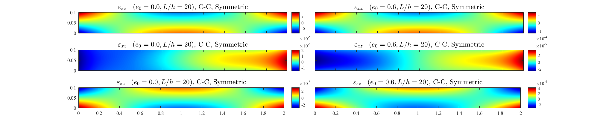
Figure 8: Strain components distribution for non-porous and porous (symmetric) beam $(L/h=20)$.

The material assumed for the porous beam is steel foam, characterized by $E_{1}=200$ GPa, $\nu=1/3$, $\rho_{1}=7850kg/m^{3}$. The beam’s cross-section has dimensions $h=0.1$ m and $b=0.1$ m (where $b$ represents the width of the beam). The validation analysis is done through a direct comparison between the present results and the work by Chen et al. [69]. Fig. 6 shows the dimensionless bending deflections $\bar{u}_{y}\ =u_{y}/h$ under a distributed load $Q=1\times 10^{4}N/m$ at the top of the beam and slenderness ratio $L/h=20$ with varying porosity coefficients. Our results are in good agreement to those reported in Chen’s study.

To observe variations in the components of stress, strain, and displacement fields within the beam, examples are provided in Figures 7, 8, and 9. Fig. 7 displays the distribution of stress components for an asymmetric beam with an H-C boundary condition. Fig. 8 illustrates the distribution of strain components for a symmetric beam with a C-C boundary condition. Finally, Fig. 9 depicts the distribution of the displacement field for an asymmetric beam with an H-H boundary condition. It should be noted that a new neural network, with the same hyperparameters, is trained for each boundary condition.

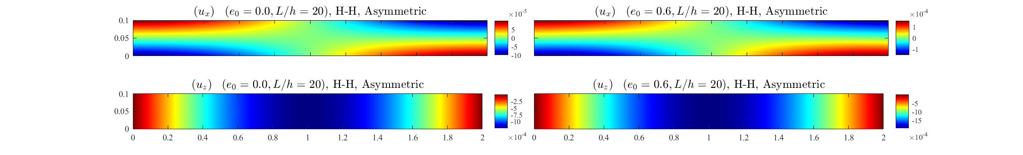
Figure 9: Displacement field distribution for non-porous and porous (asymmetric) beam $(L/h=20)$

3.3 FG Beams with arbitrary traction and porosity distribution

In this portion, we illustrate the Neural Operator in the data-driven approach discussed in section 2.3. To exemplify this, Fourier Neural Operator (FNO) has been trained to learn an operator, that maps from arbitrary traction and porosity distribution functions into the displacement field of a beam with depth $D$ and length $L$. In other words, the networks are employed to solve a range of problems with any different arbitrary traction functions and porosity distribution, which has been shown in Fig. 10. The beam is considered to be attached to supports at $x=0$ and $x=L$ and sustains a distributed load on the top edge of the beam. As a result, Eq. 38 becomes as follows:

Figure 10: Beam with Random Distributed Load and Random Porosity Distribution

$$X\coloneqq\left\{\begin{array}[]{ll}-\mathbf{\nabla}\cdot\left[\mathbf{S}\cdot\left(\mathbf{I}+\mathbf{\nabla u}\right)\right]=0\>\quad\text{for }x,\,z\in\Omega\\ \mathbf{u}(x,z)=0\,\qquad\qquad\qquad\text{ for }x=0,\,L\\ \sigma\cdot n=\hat{\mathbf{t}}\,(x)\qquad\qquad\qquad\text{for }z=D\\ \mathbf{S}=\mathbf{S}(\hat{\mathbf{E}}(z))\!\qquad\qquad\qquad\text{for }x,\,z\in\Omega\\ \end{array}\right.$$ (57)

The desired operator from this PDE is $\mathcal{G}^{\dagger}\coloneqq L^{-1}\left\{\hat{\mathbf{t}},\hat{\mathbf{E}}\right\}:\mathcal{U}^{t}\times\mathcal{U}^{E}\rightarrow\mathcal{U}$ defined to map the traction and porosity distribution to the corresponding displacement $\left\{\hat{\mathbf{t}},\hat{\mathbf{E}}\right\}\mapsto\mathbf{u}$, $\mathcal{U}^{t}$ is the space of continous real-valued functions defined on the top boundary, $\mathcal{U}^{E}$ is the space of continuous real-valued functions defined on $[0,L]*[0,D]$, and $\mathcal{U}$ is the space of continous functions with values in $\mathbb{R}^{2}$, representing the $x$- and $z$-displacements. We solve the problem when the parameters, $\Omega$ is a rectangle with corners at $(0,0)$ and $(2,0.1)$, $E_{1}=200$ GPa is Young’s modulus, $\nu=1/3$ is the Poisson ratio. For the data generation and validation, the isogeometric analysis (IGA) has been used [70] and the result for various traction functions and different porosity distributions has been compared. To provide database including the pair solution $\left\{\hat{\mathbf{t}}^{(i)},\hat{\mathbf{E}}^{(i)},\mathbf{u}^{(i)}\right\}$, we have used a Gaussian Random Fields (GRF) [71] for creating random smooth functions with a length scale $l=0.2$ for traction and a length scale $l=0.025$ for porosity distribution as

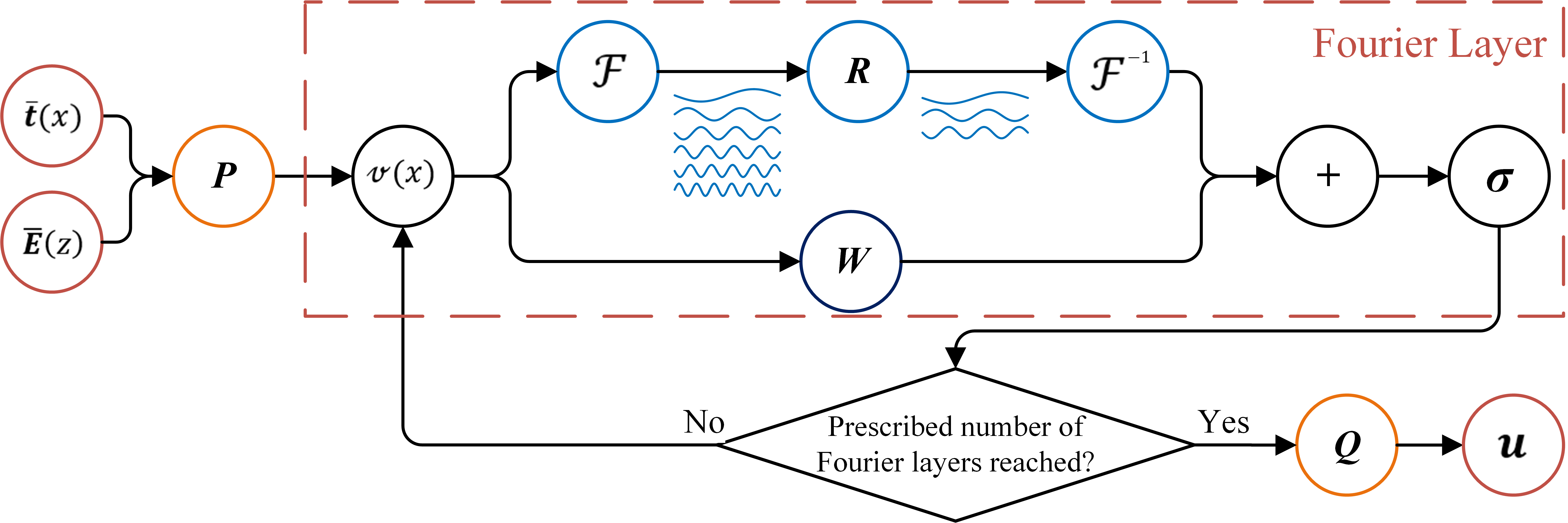
Figure 11: The architecture of the Fourier neural operators

$$\hat{\mathbf{t}}(x)\sim\sigma_{t}\times\mathcal{GP}(0,k_{1}(x_{1},x_{2}))+\mu_{t}$$ (58)

$$\hat{\mathbf{E}}(x)\sim\frac{E_{\text{max}}-E_{\text{min}}}{\mathcal{GP}_{\text{max}}-\mathcal{GP}_{\text{min}}}\times\left(\mathcal{GP}(0,k_{1}(x_{1},x_{2}))-\mathcal{GP}_{\text{min}}\right)+E_{\text{min}}$$

with an exponential quadratic covariance kernel $k_{1}(x_{1},x_{2})=\text{exp}\left(-||x_{1}-x_{2}||^{2}/(2l^{2})\right)$, where $\sigma_{t}$ and $\mu_{t}$ are expected variance and average of traction (here $\sigma_{t}=0.15$ and $\mu_{t}=0.2$), $E_{\text{min}}$ and $E_{\text{max}}$ are expected values for minimum and maximum of elasticity modulus, which in the current example are selected between 20 and 380 GPa randomly. Therefore our goal is to construct an approximation of $\mathbf{u}^{(i)}=\mathcal{G}^{\dagger}\left(\hat{\mathbf{t}}^{(i)},\hat{\mathbf{E}}^{(i)}\right)$ by the parametric map $\mathcal{G}_{\theta}:\mathcal{U}^{t}\times\mathcal{U}^{E}\rightarrow\mathcal{U},\quad\theta\in\mathbb{R}^{p}$.

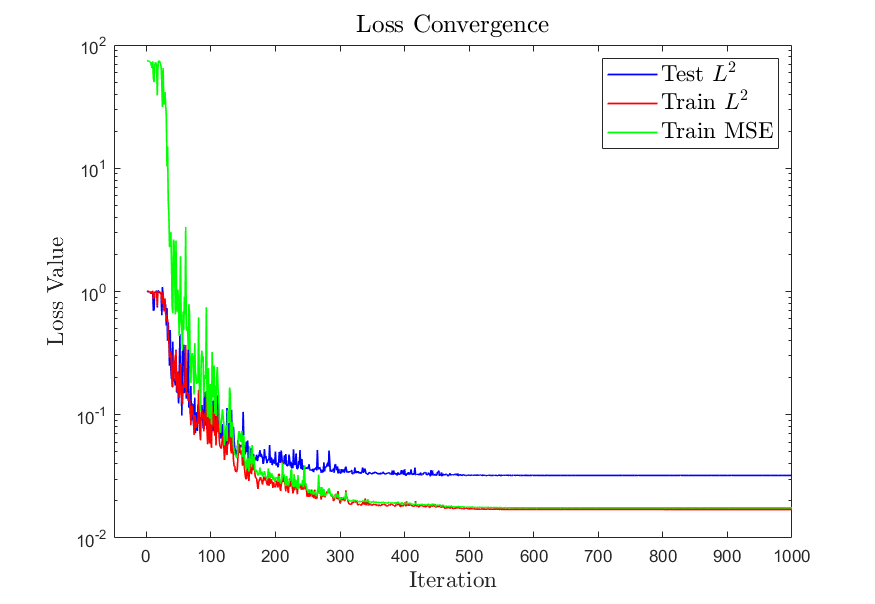
Figure 12: Convergence of the loss function.

To derive the parametric map $\mathcal{G}_{\theta}$, we utilized an FNO structured as depicted in Fig. 11. This FNO is constructed iteratively, denoted as $v_{0}\mapsto v_{1}\mapsto\ldots\mapsto v_{T}$ where $v_{j}$ for $j=0,1,\ldots,T-1$ represents a sequence of functions (Convolutional neural network) with values in $\mathbb{R}^{d_{v}}$. As illustrated in Fig. 11, the inputs $\hat{\mathbf{t}}$ and $\hat{\mathbf{E}}$ undergo a lift to a higher-dimensional representation $v_{0}(x,z)=P(\hat{\mathbf{t}})$ through a local transformation $P$, which is implemented as a 2-layer fully-connected neural network with 32 neurons in each layer. Subsequently, four Fourier layers are used, transforming $v_{t}$ to $v_{t+1}$. The final output $u(x,z)=Q(v_{T}(x,z))$ is obtained by projecting $v_{T}$ through a local transformation $Q:\mathbb{R}^{d_{v}}\mapsto\mathbb{R}^{2}$. In this case, $Q$ is a 2-hidden-layer neural network with 128 in the first layer and 2 neurons in the second layer. In addition, the Fourier layer is characterized by the following equation:

$$v_{t+1}(\chi)\coloneqq\sigma\left(W\,v_{t}(\chi)+\left(\mathcal{K}(a;\phi)\,v_{t}\right)(\chi)\right),\quad\forall\chi\in\Omega$$ (59)

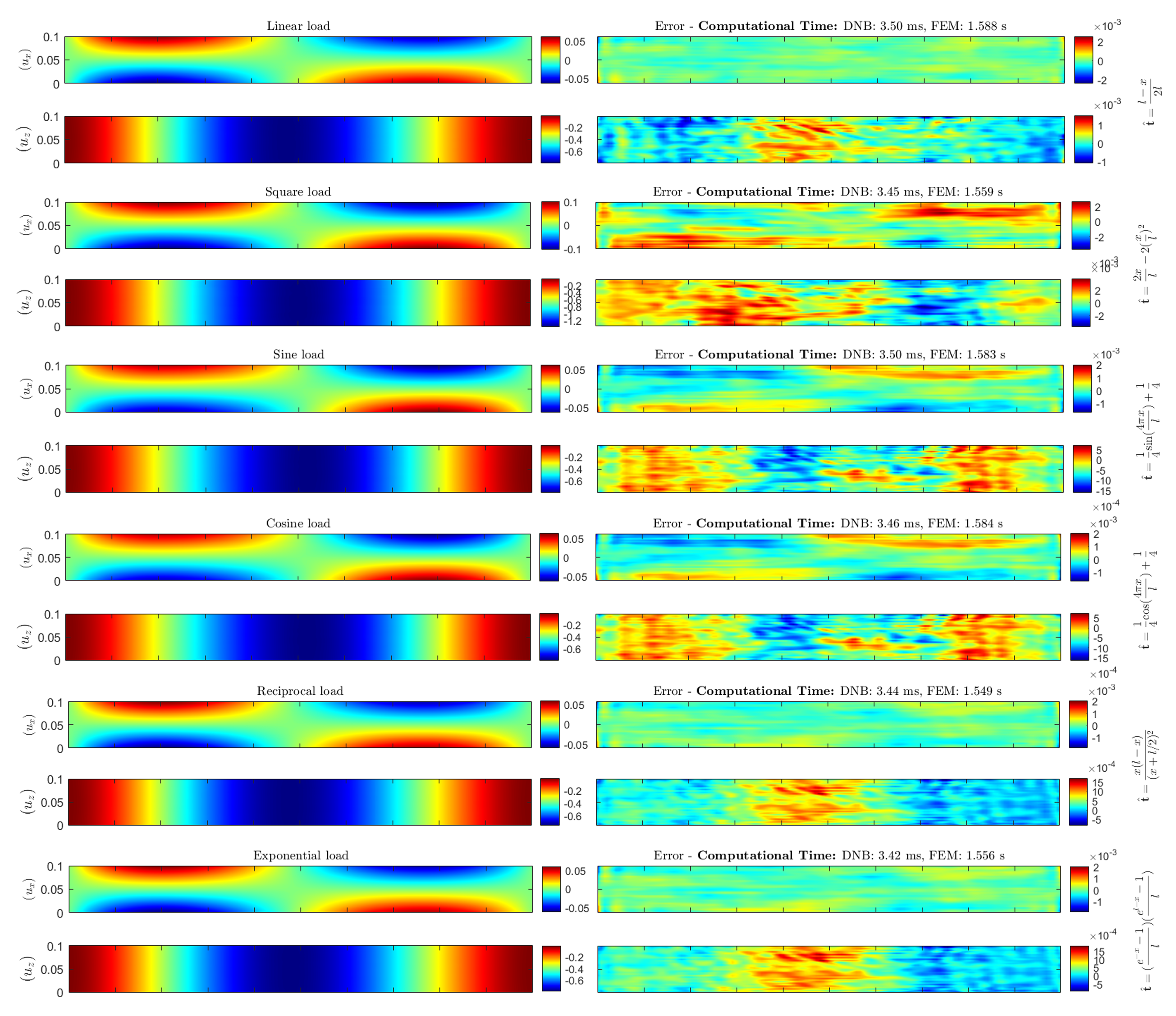
Figure 13: Displacement field distribution for different traction function and symmetric material distribution

where $\mathcal{K}:\mathcal{A}\times\Theta_{\mathcal{K}}\mapsto\mathcal{L}(\mathcal{U}(D;\mathbb{R}^{d_{v}}),\mathcal{U}(D;\mathbb{R}^{d_{v}}))$ denotes a mapping to bounded linear operators, parameterized by $\phi\in\Theta_{\mathcal{K}}$, $W:\mathbb{R}^{d_{v}}\mapsto\mathbb{R}^{d_{v}}$ is a linear transformation, and $\sigma:\mathbb{R}\mapsto\mathbb{R}$ —applied component-wise— is a non-linear activation function. Moreover, the kernel integral operator mapping in Eq. 59 is defined by

$$\left(\mathcal{K}(a;\phi)\,v_{t}\right)(\chi)=\mathcal{F}^{-1}\left(\mathcal{F}(\kappa_{\phi})\cdot\mathcal{F}(v_{t})\right)(\chi),\quad\forall\chi\in\Omega$$ (60)

where $\mathcal{F}$ denotes the Fourier transform of a function, and $\mathcal{F}^{-1}$ represents its inverse, and $\kappa_{\phi}$ is directly parameterized in Fourier space.

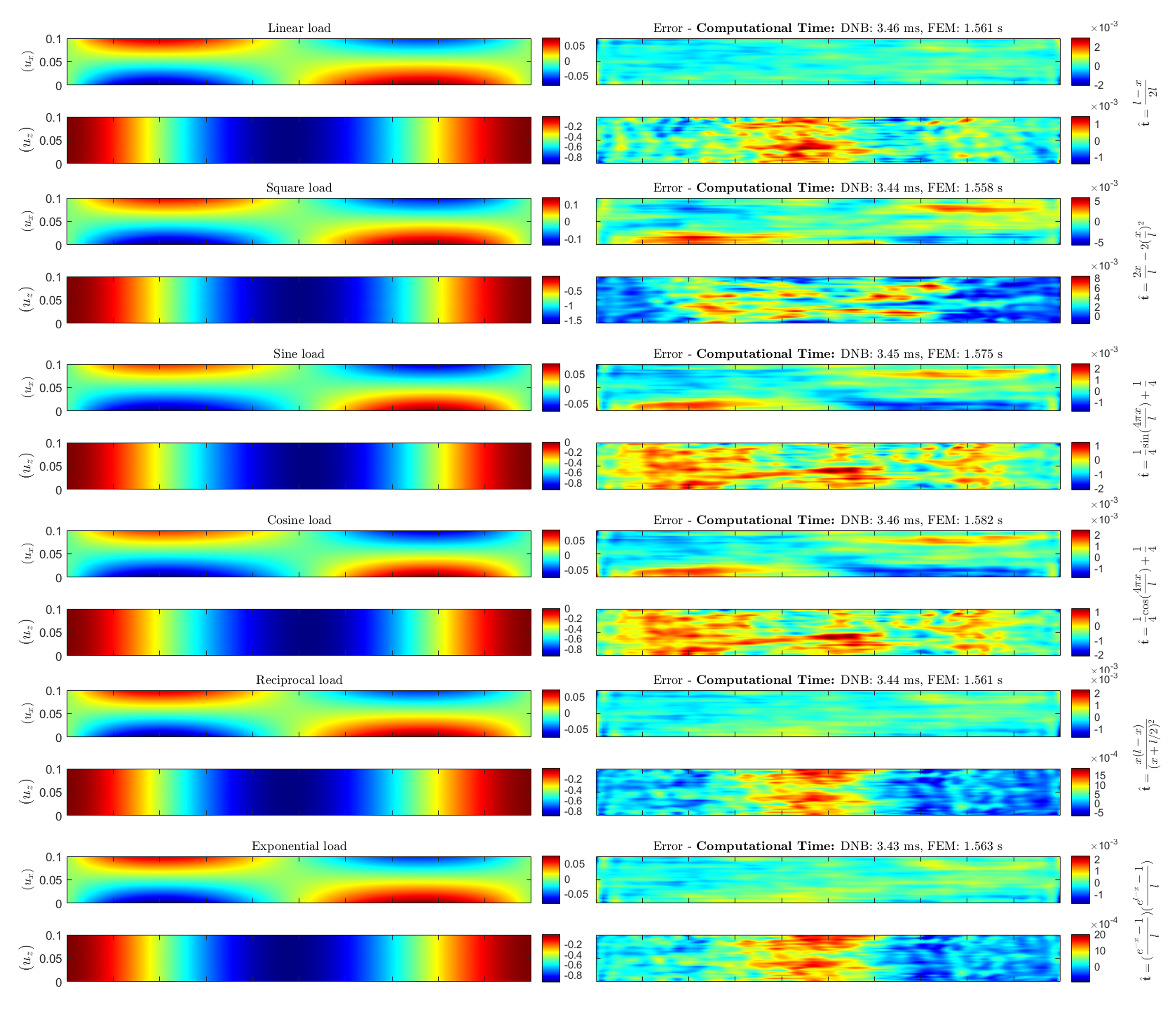
Figure 14: Displacement field distribution for different traction function and asymmetric material distribution

The displacement field was computed using $N_{x}\times N_{z}$ uniformly spaced points within the domain, with $N_{x}=128$ and $N_{z}=32$. Throughout all layers, the GELU (Gaussian Error Linear Unit) activation function was employed [72]. The optimization process utilized the Adam optimizer, and the network underwent training on 4000 sets of GRF functions and was subsequently tested on 400 additional sets of GRF functions. The computational time taken for the training part is 337 s, but once the training is complete, solving the problem with any arbitrary function takes approximately 3 milliseconds, compared to 1.5 seconds for IGA. Finally, Fig. 12 displays the convergence of the loss function, while Figs. 13-14 provides a visualization of the results obtained by employing the trained network to predict the displacement field for various traction functions and two material distributions.

4 Parametric Analysis

A comprehensive parametric analysis is conducted through a parametric study. The bending characteristics of porous beams are examined under different porosity coefficients, slenderness ratios, and various boundary conditions.

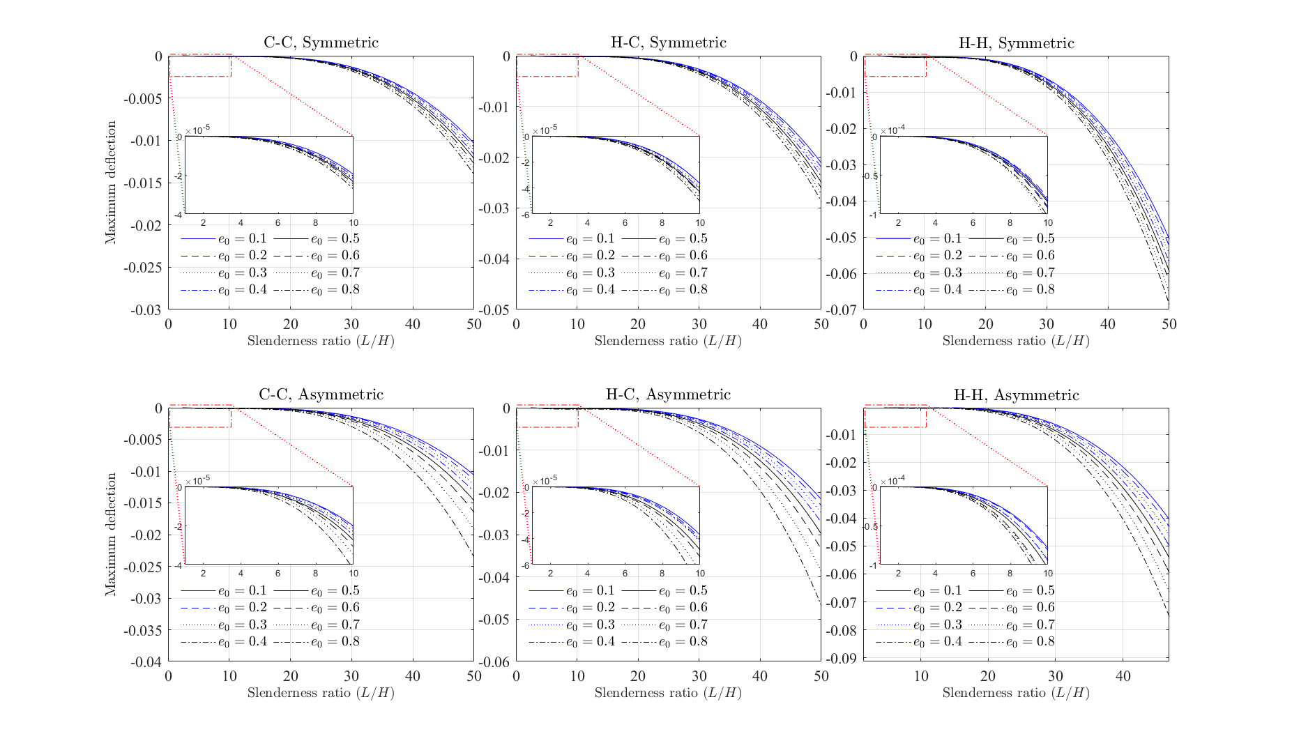
Figure 15: Maximum deflection under a uniformly distributed load: Effect of porosity coefficient and slenderness ratio

Fig. 15 depicts how the maximum deflection of a functionally graded porous beam under a uniformly distributed load is influenced by both the porosity coefficient and slenderness ratio. The graph showcases various boundary conditions and different porosity states. The trend is that increasing the porosity coefficient and slenderness ratio results in a greater deflection. Notably, beams with symmetric porosity distribution exhibit higher effective stiffness compared to those with asymmetric porosity distribution. Among the three considered boundary conditions (C-C, C-H, H-H), the H-H beam shows the largest deflection, while the C-C beam exhibits the smallest.

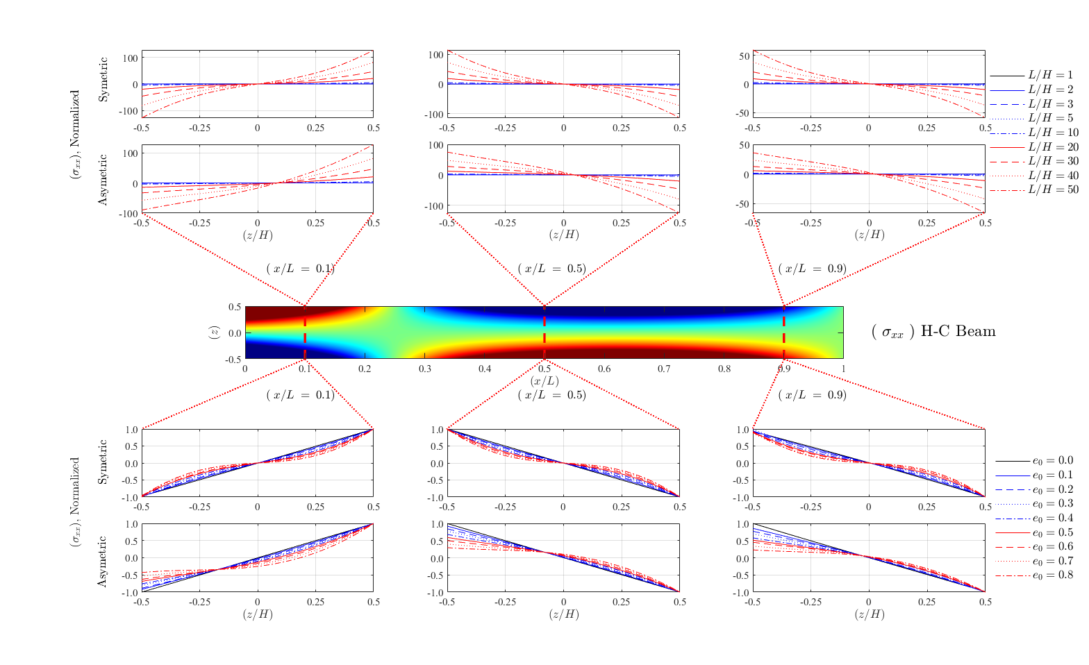
Figure 16: Effect of porosity coefficient and slenderness ratio on the variation of dimensionless normal stress through the thickness for H-C beam under a distributed load at different $x/L$.

Fig. 16 illustrates the impact of the porosity coefficient and slenderness ratio on the normalized normal stress across the thickness of an H-C beam subjected to a uniformly distributed load. Notably, the normal bending stress exhibits a linear variation along the thickness for a non-porous beam $e_{0}=0$ while it displays a nonlinear pattern for functionally graded beams due to the non-uniform porosity distribution, resulting in a nonlinear gradient in material properties.

For beams with symmetric porosity distribution, a higher porosity coefficient corresponds to larger pore size and greater internal pore intensity, leading to lower local stiffness around the midplane. Consequently, this results in lower normal stress in the midplane region and higher stress on both the top and bottom surfaces. The normal bending stress is symmetric about the mid-plane for symmetric porosity distribution but asymmetric for asymmetric porosity distribution, where the pore size gradually increases from the top surface to the bottom surface. As a consequence, the maximum normal bending stress on the top surface is significantly larger than that on the bottom surface, with the difference increasing as $e_{0}$ rises. Additionally, as expected, slender beams exhibit higher normal bending stress due to their weaker bending stiffness and larger deflections.

It is important to note that the aforementioned observations regarding normal bending stress, specifically for an H-H beam under a distributed load, are applicable to beams with various boundary and loading conditions, although those are not detailed here for conciseness.

5 Conclusion

The study investigated the application of scientific machine learning techniques, such as PINNs, DEM, and Neural Operators for functionally graded porous beam analysis for functionally graded porous beam analysis and unified them under one framework, named DeepNetBeam (DNB). This framework significantly improves the accuracy of beam analysis by minimizing reliance on the assumptions inherent to other beam theories. Through application in the analysis of FG porous beams, DNB showcases its versatility. Adopting SciML techniques ensures the efficient training of neural networks, yielding accurate results. Comparative analysis with exact solutions validates the efficacy of the methods, while the application of Neural Operators demonstrates a speed-up compared to traditional methods, notably in problems with arbitrary traction and material distribution. Parametric investigations on porous beams offer insights into the impact of parameters such as slenderness ratio and porosity coefficient on bending characteristics.

Finally, this paper introduces a framework and demonstrates its applicability in structural analysis. By significantly reducing reliance on assumptions and showcasing efficient numerical solutions, it provides an opportunity for more accurate analysis of beam-like structures. The outcomes emphasize the potential of DNB in shaping the future of accurate and efficient structural analysis methodologies.

Declaration of Competing Interest

The authors declare that they have no known competing financial interests or personal relationships that could have appeared to influence the work reported in this paper.

References

- [1] Yan Li et al. “A review on functionally graded materials and structures via additive manufacturing: from multi-scale design to versatile functional properties” In Advanced Materials Technologies 5.6 Wiley Online Library, 2020, pp. 1900981 DOI: 10.1002/admt.201900981
- [2] L Audouard et al. “Resistance of ceramic/metal Functionally Graded Materials in the flame of a combustion chamber under harsh thermal and environmental conditions” In Materials Characterization 208 Elsevier, 2024, pp. 113616 DOI: 10.1016/j.matchar.2023.113616
- [3] René Daniel Pütz et al. “Microstructure and corrosion behavior of functionally graded wire arc additive manufactured steel combinations” In Steel Research International 92.12 Wiley Online Library, 2021, pp. 2100387 DOI: 10.1002/srin.202100387
- [4] Andreas Öchsner and Andreas Öchsner “Euler–Bernoulli Beam Theory” In Classical Beam Theories of Structural Mechanics Springer, 2021, pp. 7–66 DOI: 10.1007/978-3-030-76035-9
- [5] M Mohammadimehr et al. “Bending, buckling, and free vibration analyses of carbon nanotube reinforced composite beams and experimental tensile test to obtain the mechanical properties of nanocomposite” In Steel Compos. Struct., Int. J 29.3, 2018, pp. 405–422 DOI: 10.12989/scs.2018.29.3.405
- [6] Perampalam Gatheeshgar et al. “Optimised cold-formed steel beams in modular building applications” In Journal of Building Engineering 32 Elsevier, 2020, pp. 101607 DOI: 10.1016/j.jobe.2020.101607
- [7] Masoud Babaei, Faraz Kiarasi, Kamran Asemi and Mohammad Hosseini “Functionally graded saturated porous structures: A review” In Journal of Computational Applied Mechanics 53.2 University of Tehran, 2022, pp. 297–308 DOI: 10.22059/JCAMECH.2022.342710.719
- [8] Prashik Malhari Ramteke and Subrata Kumar Panda “Computational modelling and experimental challenges of linear and nonlinear analysis of porous graded structure: a comprehensive review” In Archives of Computational Methods in Engineering 30.5 Springer, 2023, pp. 3437–3452 DOI: 10.1007/s11831-023-09908-x
- [9] Da Chen, Jie Yang and Sritawat Kitipornchai “Free and forced vibrations of shear deformable functionally graded porous beams” In International journal of mechanical sciences 108 Elsevier, 2016, pp. 14–22 DOI: 10.1016/j.ijmecsci.2016.01.025
- [10] Faraz Kiarasi et al. “A review on functionally graded porous structures reinforced by graphene platelets” In J. Comput. Appl. Mech 52.4, 2021, pp. 731–750 DOI: 10.22059/JCAMECH.2021.335739.675
- [11] Da Chen, Kang Gao, Jie Yang and Lihai Zhang “Functionally graded porous structures: Analyses, performances, and applications–A Review” In Thin-Walled Structures 191 Elsevier, 2023, pp. 111046 DOI: 10.1016/j.tws.2023.111046
- [12] S Agarwal, A Chakraborty and S Gopalakrishnan “Large deformation analysis for anisotropic and inhomogeneous beams using exact linear static solutions” In Composite structures 72.1 Elsevier, 2006, pp. 91–104 DOI: 10.1016/j.compstruct.2004.10.019
- [13] Ali Fallah and Mohammad Mohammadi Aghdam “Physics-informed neural network for bending and free vibration analysis of three-dimensional functionally graded porous beam resting on elastic foundation” In Engineering with Computers Springer, 2023, pp. 1–18 DOI: 10.1007/s00366-023-01799-7
- [14] Muhittin Turan, Ecren Uzun Yaylacı and Murat Yaylacı “Free vibration and buckling of functionally graded porous beams using analytical, finite element, and artificial neural network methods” In Archive of Applied Mechanics 93.4 Springer, 2023, pp. 1351–1372 DOI: 10.1007/s00419-022-02332-w
- [15] Vien Minh Nguyen-Thanh et al. “Parametric deep energy approach for elasticity accounting for strain gradient effects” In Computer Methods in Applied Mechanics and Engineering 386 Elsevier, 2021, pp. 114096 DOI: 10.1016/j.cma.2021.114096
- [16] Esteban Samaniego et al. “An energy approach to the solution of partial differential equations in computational mechanics via machine learning: Concepts, implementation and applications” In Computer Methods in Applied Mechanics and Engineering 362 Elsevier, 2020, pp. 112790 DOI: 10.1016/j.cma.2019.112790
- [17] Farzad Ebrahimi and Hosein Ezzati “A Machine-Learning-Based Model for Buckling Analysis of Thermally Affected Covalently Functionalized Graphene/Epoxy Nanocomposite Beams” In Mathematics 11.6 MDPI, 2023, pp. 1496 DOI: 10.3390/math11061496
- [18] Asif Ahmed et al. “Prediction of shear behavior of glass FRP bars-reinforced ultra-highperformance concrete I-shaped beams using machine learning” In International Journal of Mechanics and Materials in Design Springer, 2023, pp. 1–22 DOI: 10.1007/s10999-023-09675-4
- [19] Seyed Mohammad Mojtabaei, Jurgen Becque, Iman Hajirasouliha and Rasoul Khandan “Predicting the buckling behaviour of thin-walled structural elements using machine learning methods” In Thin-Walled Structures 184 Elsevier, 2023, pp. 110518 DOI: 10.1016/j.tws.2022.110518
- [20] Jan Blechschmidt and Oliver G Ernst “Three ways to solve partial differential equations with neural networks—A review” In GAMM-Mitteilungen 44.2 Wiley Online Library, 2021, pp. e202100006 DOI: 10.1002/gamm.202100006
- [21] Lucie P Aarts and Peter Van Der Veer “Neural network method for solving partial differential equations” In Neural Processing Letters 14 Springer, 2001, pp. 261–271 DOI: 10.1023/A:1012784129883
- [22] Tim Dockhorn “A discussion on solving partial differential equations using neural networks” In arXiv preprint arXiv:1904.07200, 2019 DOI: 10.48550/arXiv.1904.07200
- [23] Christian Beck, Martin Hutzenthaler, Arnulf Jentzen and Benno Kuckuck “An overview on deep learning-based approximation methods for partial differential equations” In arXiv preprint arXiv:2012.12348, 2020 DOI: 10.48550/arXiv.2012.12348
- [24] Neha Yadav, Anupam Yadav and Manoj Kumar “An introduction to neural network methods for differential equations” Springer, 2015 DOI: 10.1007/978-94-017-9816-7
- [25] Salvatore Cuomo et al. “Scientific machine learning through physics–informed neural networks: Where we are and what’s next” In Journal of Scientific Computing 92.3 Springer, 2022, pp. 88 DOI: 10.1007/s10915-022-01939-z
- [26] Tony Hey, Keith Butler, Sam Jackson and Jeyarajan Thiyagalingam “Machine learning and big scientific data” In Philosophical Transactions of the Royal Society A 378.2166 The Royal Society Publishing, 2020, pp. 20190054 DOI: 10.1098/rsta.2019.0054
- [27] Maziyar Bazmara, Mohammad Mianroodi and Mohammad Silani “Application of Physics-informed neural networks for nonlinear buckling analysis of beams” In Acta Mechanica Sinica 39.6 Springer, 2023, pp. 422438 DOI: 10.1007/s10409-023-22438-x
- [28] Ehsan Haghighat et al. “A physics-informed deep learning framework for inversion and surrogate modeling in solid mechanics” In Computer Methods in Applied Mechanics and Engineering 379 Elsevier, 2021, pp. 113741 DOI: 10.1016/j.cma.2021.113741
- [29] Cosmin Anitescu, Burak İsmail Ateş and Timon Rabczuk “Physics-Informed Neural Networks: Theory and Applications” In Machine Learning in Modeling and Simulation: Methods and Applications Springer, 2023, pp. 179–218 DOI: 10.1007/978-3-031-36644-4˙5
- [30] Taniya Kapoor, Hongrui Wang, Alfredo Núñez and Rolf Dollevoet “Physics-Informed Neural Networks for Solving Forward and Inverse Problems in Complex Beam Systems” In IEEE Transactions on Neural Networks and Learning Systems, 2023, pp. 1–15 DOI: 10.1109/TNNLS.2023.3310585
- [31] Arunabha M Roy, Rikhi Bose, Veera Sundararaghavan and Raymundo Arróyave “Deep learning-accelerated computational framework based on Physics Informed Neural Network for the solution of linear elasticity” In Neural Networks 162 Elsevier, 2023, pp. 472–489 DOI: 10.1016/j.neunet.2023.03.014
- [32] Somdatta Goswami, Cosmin Anitescu, Souvik Chakraborty and Timon Rabczuk “Transfer learning enhanced physics informed neural network for phase-field modeling of fracture” In Theoretical and Applied Fracture Mechanics 106 Elsevier, 2020, pp. 102447 DOI: 10.1016/j.tafmec.2019.102447
- [33] Khang A Luong, Thang Le-Duc and Jaehong Lee “Deep reduced-order least-square method—A parallel neural network structure for solving beam problems” In Thin-Walled Structures 191 Elsevier, 2023, pp. 111044
- [34] Vien Minh Nguyen-Thanh, Xiaoying Zhuang and Timon Rabczuk “A deep energy method for finite deformation hyperelasticity” In European Journal of Mechanics-A/Solids 80 Elsevier, 2020, pp. 103874 DOI: 10.1016/j.euromechsol.2019.103874
- [35] Huanhuan Gao et al. “DHEM: a deep heat energy method for steady-state heat conduction problems” In Journal of Mechanical Science and Technology Springer, 2022, pp. 1–15 DOI: 10.1007/s12206-022-1039-0
- [36] Jan N Fuhg and Nikolaos Bouklas “The mixed deep energy method for resolving concentration features in finite strain hyperelasticity” In Journal of Computational Physics 451 Elsevier, 2022, pp. 110839 DOI: 10.1016/j.jcp.2021.110839
- [37] Takashi Matsubara, Ai Ishikawa and Takaharu Yaguchi “Deep energy-based modeling of discrete-time physics” In Advances in Neural Information Processing Systems 33, 2020, pp. 13100–13111
- [38] Xiaoying Zhuang et al. “Deep autoencoder based energy method for the bending, vibration, and buckling analysis of Kirchhoff plates with transfer learning” In European Journal of Mechanics-A/Solids 87 Elsevier, 2021, pp. 104225 DOI: 10.1016/j.euromechsol.2021.104225
- [39] Diab W Abueidda, Seid Koric, Erman Guleryuz and Nahil A Sobh “Enhanced physics-informed neural networks for hyperelasticity” In International Journal for Numerical Methods in Engineering 124.7 Wiley Online Library, 2023, pp. 1585–1601 DOI: 10.1002/nme.7176
- [40] Junyan He, Diab Abueidda, Seid Koric and Iwona Jasiuk “On the use of graph neural networks and shape-function-based gradient computation in the deep energy method” In International Journal for Numerical Methods in Engineering 124.4 Wiley Online Library, 2023, pp. 864–879 DOI: 10.1002/nme.7146
- [41] Junyan He et al. “A deep learning energy-based method for classical elastoplasticity” In International Journal of Plasticity Elsevier, 2023, pp. 103531 DOI: 10.1016/j.ijplas.2023.103531
- [42] Arvin Mojahedin, Mohammad Salavati and Timon Rabczuk “A deep energy method for functionally graded porous beams” In Journal of Zhejiang University-SCIENCE A 22.6 Springer, 2021, pp. 492–498 DOI: 10.1631/jzus.A1900888
- [43] Arvin Mojahedin et al. “A Deep Energy Method for the Analysis of Thermoporoelastic Functionally Graded Beams” In International Journal of Computational Methods 19.08 World Scientific, 2022, pp. 2143020 DOI: 10.1142/S0219876221430209
- [44] Nikola Kovachki et al. “Neural Operator: Learning Maps Between Function Spaces With Applications to PDEs” In Journal of Machine Learning Research 24.89, 2023, pp. 1–97 URL: http://jmlr.org/papers/v24/21-1524.html
- [45] Junuthula Narasimha Reddy “Theories and analyses of beams and axisymmetric circular plates” CRC Press, 2022 DOI: 10.1201/9781003240846
- [46] Junuthula Narasimha Reddy “An introduction to continuum mechanics” Cambridge university press, 2013 DOI: 10.1017/CBO9781139178952
- [47] Marta Lewicka, Lakshminarayanan Mahadevan and Mohammad Reza Pakzad “The Föppl-von Kármán equations for plates with incompatible strains” In Proceedings of the Royal Society A: Mathematical, Physical and Engineering Sciences 467.2126 The Royal Society Publishing, 2011, pp. 402–426 DOI: 10.1098/rspa.2010.0138
- [48] Martin H Sadd “Elasticity: theory, applications, and numerics” Academic Press, 2009 DOI: 10.1016/C2012-0-06981-5
- [49] Shmuel Livio Weissman “A unified approach to mixed finite element methods” University of California, Berkeley, 1990
- [50] Jihuan He “Equivalent theorem of Hellinger-Reissner and Hu-Washizu variational principles” In Journal of Shanghai University (English Edition) 1 Springer, 1997, pp. 36–41 DOI: 10.1007/s11741-997-0041-1
- [51] Sebastian Ruder “An overview of gradient descent optimization algorithms” In arXiv preprint arXiv:1609.04747, 2016 DOI: 10.48550/arXiv.1609.04747
- [52] Diederik P Kingma and Jimmy Ba “Adam: A method for stochastic optimization” In arXiv preprint arXiv:1412.6980, 2014 DOI: 10.48550/arXiv.1412.6980
- [53] Wei Zhao “A Broyden–Fletcher–Goldfarb–Shanno algorithm for reliability-based design optimization” In Applied Mathematical Modelling 92 Elsevier, 2021, pp. 447–465 DOI: 10.1016/j.apm.2020.11.012
- [54] Yunhai Xiao, Zengxin Wei and Zhiguo Wang “A limited memory BFGS-type method for large-scale unconstrained optimization” In Computers & Mathematics with Applications 56.4 Elsevier, 2008, pp. 1001–1009 DOI: 10.1016/j.camwa.2008.01.028
- [55] Gaurav Gupta, Xiongye Xiao and Paul Bogdan “Multiwavelet-based operator learning for differential equations” In Advances in neural information processing systems 34, 2021, pp. 24048–24062 DOI: https://doi.org/10.48550/arXiv.2109.13459
- [56] Md Ashiqur Rahman, Zachary E Ross and Kamyar Azizzadenesheli “U-NO: U-shaped Neural Operators” In arXiv e-prints, 2022, pp. arXiv–2204 DOI: https://doi.org/10.48550/arXiv.2204.11127
- [57] Zongyi Li et al. “Multipole graph neural operator for parametric partial differential equations” In Advances in Neural Information Processing Systems 33, 2020, pp. 6755–6766
- [58] Zongyi Li et al. “Fourier Neural Operator for Parametric Partial Differential Equations”, 2021 DOI: 10.48550/arXiv.2010.08895
- [59] Lu Lu et al. “Learning nonlinear operators via DeepONet based on the universal approximation theorem of operators” In Nature Machine Intelligence 3.3 Springer ScienceBusiness Media LLC, 2021, pp. 218–229 DOI: 10.1038/s42256-021-00302-5
- [60] Stephen Timoshenko “Theory of elasticity” Oxford, 1951
- [61] Prajit Ramachandran, Barret Zoph and Quoc V Le “Searching for activation functions” In arXiv preprint arXiv:1710.05941, 2017 DOI: 10.48550/arXiv.1710.05941
- [62] Chenxi Wu et al. “A comprehensive study of non-adaptive and residual-based adaptive sampling for physics-informed neural networks” In Computer Methods in Applied Mechanics and Engineering 403 Elsevier, 2023, pp. 115671 DOI: https://doi.org/10.1016/j.cma.2022.115671
- [63] Michael D McKay, Richard J Beckman and William J Conover “A comparison of three methods for selecting values of input variables in the analysis of output from a computer code” In Technometrics 42.1 Taylor & Francis, 2000, pp. 55–61 DOI: https://doi.org/10.2307/1268522
- [64] John H Halton “On the efficiency of certain quasi-random sequences of points in evaluating multi-dimensional integrals” In Numerische Mathematik 2 Springer, 1960, pp. 84–90 DOI: https://doi.org/10.1007/BF01386213
- [65] JM Hammersley and DC Handscomb “Monte Carlo methods” In Ltd., London 40, 1964, pp. 32 DOI: https://doi.org/10.1007/978-94-009-5819-7
- [66] Il’ya Meerovich Sobol’ “On the distribution of points in a cube and the approximate evaluation of integrals” In Zhurnal Vychislitel’noi Matematiki i Matematicheskoi Fiziki 7.4 Russian Academy of Sciences, Branch of Mathematical Sciences, 1967, pp. 784–802 DOI: https://doi.org/10.1016/0041-5553(67)90144-9
- [67] Krzysztof Magnucki and Piotr Stasiewicz “Elastic buckling of a porous beam” In Journal of theoretical and applied mechanics 42.4, 2004, pp. 859–868 DOI: http://www.ptmts.org.pl/jtam/index.php/jtam/article/view/v42n4p859
- [68] M Jabbari, A Mojahedin, AR Khorshidvand and MR Eslami “Buckling analysis of a functionally graded thin circular plate made of saturated porous materials” In Journal of Engineering Mechanics 140.2 American Society of Civil Engineers, 2014, pp. 287–295 DOI: 10.1061/(ASCE)EM.1943-7889.0000663
- [69] Dong Chen, Jie Yang and S Kitipornchai “Elastic buckling and static bending of shear deformable functionally graded porous beam” In Composite Structures 133 Elsevier, 2015, pp. 54–61 DOI: 10.1016/j.compstruct.2015.07.052
- [70] Cosmin Anitescu, Md Naim Hossain and Timon Rabczuk “Recovery-based error estimation and adaptivity using high-order splines over hierarchical T-meshes” In Computer Methods in Applied Mechanics and Engineering 328 Elsevier, 2018, pp. 638–662 DOI: 10.1016/j.cma.2017.08.032
- [71] Christopher KI Williams and Carl Edward Rasmussen “Gaussian processes for machine learning” MIT press Cambridge, MA, 2006 DOI: 10.7551/mitpress/3206.001.0001
- [72] Dan Hendrycks and Kevin Gimpel “Gaussian error linear units (GELUs)” In arXiv preprint arXiv:1606.08415, 2016 DOI: 10.48550/arXiv.1606.08415