Randomized Transport Plans via Hierarchical Fully Probabilistic Design

Abstract

An optimal randomized strategy for design of balanced, normalized mass transport plans is developed. It replaces—but specializes to—the deterministic, regularized optimal transport (OT) strategy, which yields only a certainty-equivalent plan. The incompletely specified—and therefore uncertain—transport plan is acknowledged to be a random process. Therefore, hierarchical fully probabilistic design (HFPD) is adopted, yielding an optimal hyperprior supported on the set of possible transport plans, and consistent with prior mean constraints on the marginals of the uncertain plan. This Bayesian resetting of the design problem for transport plans —which we call HFPD-OT — confers new opportunities. These include (i) a strategy for the generation of a random sample of joint transport plans; (ii) randomized marginal contracts for individual source-target pairs; and (iii) consistent measures of uncertainty in the plan and its contracts. An application in algorithmic fairness is outlined, where HFPD-OT enables the recruitment of a more diverse subset of contracts—than is possible in classical OT—into the delivery of an expected plan. Also, it permits fairness proxies to be endowed with uncertainty quantifiers.

Keywords— Optimal transport, Bayesian hierarchical modelling, Fully probabilistic design, Convex optimization, Allocation, Algorithmic fairness

1 Main Contributions

Optimal transport (OT) refers to the classical design of a deterministic transport plan, $\pi$, for taking a unit mass—distributed across a source domain, $\mathbb{\mathbb{\Omega}}_{X}$—and redistributing it across a target domain, $\mathbb{\mathbb{\Omega}}_{Y}$. The transport plan is expressed as an unknown, deterministic, joint distribution, $\pi$, with support in $\mathbb{\mathbb{\Omega}}_{X}\times\mathbb{\mathbb{\Omega}}_{Y}$. The distributed source and target are therefore the marginals of $\pi$, and are specified a priori by $\mu_{0}$ and $\nu_{0}$ on $\mathbb{\mathbb{\Omega}}_{X}$ and $\mathbb{\mathbb{\Omega}}_{Y}$, respectively. Consequently, $\pi$ in confined to the space, $\mathbb{\Pi}(\mu_{0},\nu_{0})$, of distributions on $\mathbb{\mathbb{\Omega}}_{X}\times\mathbb{\mathbb{\Omega}}_{Y}$, with $\mu_{0}$ and $\nu_{0}$ as its marginals. An optimal choice, $\pi^{o}$, of $\pi$—called the OT plan—is achieved by minimizing the expected value, under $\pi$, of a pre-specified cost of transport, ${\mathsf{C}}(x,y)$, from $\mathbb{\mathbb{\Omega}}_{X}$ to $\mathbb{\mathbb{\Omega}}_{Y}$.

In this paper, we reformulate the design of transport maps in the Bayesian (i.e. fully probabilistic) way. In particular, deterministic optimization—yielding $\pi^{o}$—is replaced by the hierarchical fully probabilistic design (HFPD) of an optimal randomized decision-making strategy, $\pi\sim\mathsf{S}^{o}$ (i.e. a hyperprior), for choosing $\pi$. This approach recognizes that the unknown transport plan, $\pi$, is a (generally nonparametric) random process. Therefore, we equip it with a prior, $\mathsf{S}(\pi|K)$, where $K$ denotes marginal (mean) knowledge constraints which will be detailed in the sequel. Following the axioms of FPD at this hierarchical level (i.e. HFPD), we equip the space, ${\mathbb{S}}_{K}$, of $\mathsf{S}$—being the randomized strategy for choosing the transport plan, $\pi$—with an appropriately formulated loss function, and we minimize the expected value of the latter under $\mathsf{S}$. This yields the optimal randomized strategy, $\mathsf{S}^{o}$, for choosing $\pi$, being also the optimal hyperprior for uncertain $\pi$. We show that this is equivalent to minimization of a Kullback-Leibler divergence (KLD), leading to a Gibbs form for $\mathsf{S}^{o}$:

$$\mathsf{S}^{o}(\pi|K)\propto\mathsf{S}_{\mathsf{I}}(\pi|K)e^{-{\mathsf{D}_{\mathsf{KL}}}(\pi||\pi_{\mathsf{I}})}e^{-\lambda_{1}^{o}{\mathsf{D}_{\mathsf{KL}}}(\mu||\mu_{0})}e^{-\lambda_{2}^{o}{\mathsf{D}_{\mathsf{KL}}}(\nu||\nu_{0})}\in{\mathbb{S}}_{K}.$$ (1)

Here, $\mu$ and $\nu$ are the random (i.e. uncertain) marginals of the random transport plan, $\pi$. The KLDs, ${\mathsf{D}_{\mathsf{KL}}}(\cdot||\cdot)$, act as Gibbs energies. Meanwhile, $\mathsf{S}_{\mathsf{I}}$ and $\pi_{\mathsf{I}}$ are the freely but necessarily pre-specified zero-loss choices of $\mathsf{S}$ and $\pi$, respectively, referred to as the ideal or target choices.

By resetting OT as a problem of Bayesian decision making via HFPD, we achieve the following principal goals:

• The deterministic, regularized OT choice, $\pi^{o}$, obtained via constrained optimization at the base level of modelling, $(x,y)\sim\pi$, is replaced by an optimal generator of randomized plans (i.e. a randomized strategy for designing transport plans, $\pi$) at the hierarchical level of complete modelling , $\pi\sim\mathsf{S}^{o}$.

• In the parametric case, in which the set, ${\mathbb{\mathbb{\Omega}}_{X}}\times{\mathbb{\mathbb{\Omega}}_{Y}}$, of source-target states—which we call contracts—is (countably) finite, we can compute optimal (marginal and/or conditional) distributions, $\pi_{i,j}\sim\mathsf{S}^{o}_{i,j}$, for modelling and randomization of the transport contract from $x_{i}$ to $y_{j}$.

• In line with all Bayesian decision-making strategies, we can summarize $\pi\sim\mathsf{S}^{o}$ via a certainty-equivalent (CE) transport plan, $\hat{\pi}\in\mathbb{\Pi}_{K}$—such as its expected or maximally probable value—and equip this with a summary of our uncertainty in $\pi$ (e.g. via the Bayesian standard intervals for the contracts, $\pi_{i,j}\sim\mathsf{S}^{o}_{i,j}$).

By way of demonstrating the significant potential for this HFPD resetting of OT, we consider an application in algorithmic fairness. We show how the randomization of transport plans can improve diversity among contracts, and equip fairness proxies with measures of uncertainty.

2 Introduction to transport plan design and optimal transport

Optimal Transport (OT) techniques have received increasing attention in the past decade, in a wide range of domains such as machine learning and generative adversarial learning [Arjovsky et al., 2017], domain adaptation [Courty et al., 2017], image processing and watermarking [Mathon et al., 2014], hallucination detection in neural translation machines [Guerreiro et al., 2023], etc. In addition to traditional applications in economics and data matching [Galichon, 2016], fluid mechanics and diffusion processes [Saumier et al., 2015], it has also been used to perform sampling and Bayesian inference [El Moselhy and Marzouk, 2012].

OT is concerned with the least costly transport plan (in expectation) between a source and a target probability measure. The unregularized OT plan induces a natural distance in the space of probability measures (the Wasserstein-Rubinstein distance) [Villani, 2008], introducing a rich topological structure by lifting key geometric properties associated with the ground metric to the space of probability measures [Villani, 2008, Peyré and Cuturi, 2019]. For example, if the ground space is Euclidean, concepts like gradient, barycentre and convexity are naturally extended to the space of probability measures.

Notwithstanding the wide range of applications, the classical formalism of OT confines it to a purely deterministic setting, which regards the transport plan as a crisp object and assumes perfect knowledge of the marginals (Figure 1(a)). It fails to model and (critically) translate uncertainty in the marginals to uncertainty in the design of transport plans. In this regard, classical OT is an instance of certainty-equivalence (CE) decision making, which produces myopic transport strategies that do not account for the uncertain and random nature of many real systems. One might think that recasting the classical OT problem in terms of robust optimization might address these issues. A robust optimization formulation relies on a deterministic, unknown but bounded description of the uncertainty in the marginals [Ben-Tal et al., 2009]. Such a design choice may be overly conservative: it indeed considers all possible outcomes in the uncertainty set, but may assign non-negligible weights even to plans that are highly improbable. Furthermore, the robust design is not equipped with a quantifier of the intrinsic uncertainty of the transport plan.

In this paper, we propose the HFPD-OT approach to the design of uncertain transport plans. It departs from the classical, base-level OT setting by regarding the transport plan as a random process. Consistent hierarchical Bayesian modelling endows the uncertain plan with its own hyperprior (Figure 1(b)). Its optimal choice provides a randomized strategy for choosing transport plans in the space of plans consistent with prior-imposed knowledge constraints on its marginals. It also acts as a generative model for random sampling of transport plans. By treating transport plans as random processes, we effectively recast the transport design problem as one of inference. This contrasts with the OT literature, which is only concerned with deterministic optimization strategies for choosing deterministic plans. As we will see in the literature review, next, the tools provided by HFPD-OT—intended for modelling and reasoning about uncertainty in transport plans—are not available in the classical OT setting.

2.1 Approaches to modelling uncertainty in OT

There are precedents in eliciting and processing uncertainty in OT, but they are generally couched in terms of base-level modelling, and not in terms of the hierarchical Bayesian approach developed here. Specifically, (i) our method is primarily concerned with the design of a fully probabilistic model over the space of transport plans; (ii) as such, the transport plan is modelled as a (generally nonparametric) process endowed with its own (hyper)prior; and (iii) we rely on randomization techniques for choosing plans, in contrast to existing methods which are mainly based on deterministic optimization techniques.

Copulas [Sklar, 1959] are historically among the first methods proposed for the design of multivariate distributions with arbitrary, but perfectly known marginals. Other techniques relaxed this assumption to address situations where exactly one marginal is uncertain. This is the case in [Goodman, 1953], for instance, where the authors model the uncertainty in one marginal with a Gaussian noise. In ecological inference (a case of parametric transport design on a finite support), [Wakefield, 2004] studied the case where one marginal is uncertain, adopting a hierarchical multinomial-Dirichlet-based model. We highlight two distinctions in our work: (i) we do not impose a parametric constraint in general, and we allow for uncertainty in both marginals; and (ii) the authors of the earlier paper pursue markedly different statistical inference objectives from OT .

Interestingly, the connection between ecological inference and OT was not established until later, in [Frogner and Poggio, 2019], where the authors extended the previous model and studied the case where both marginals are uncertain. The questions we address in this paper again differ from those in [Frogner and Poggio, 2019] in the following ways: (i) they solve a base-level MAP optimization problem using a Bregman projection method, once again recovering a certainty-equivalent OT plan, whereas our primary goal is to depart from such a certainty-equivalence framework and design an optimal hierarchical Bayesian model from which random transport plans can be generated and used in lieu of an OT plan. If required (as we will see), the expected plan takes the place of the MAP plan as the Bayesian minimum-risk decision (i.e. estimate) of the uncertain plan, with asymptotic convergence to the MAP plan; and (ii) the derivations in [Frogner and Poggio, 2019] rely on parametric and structural assumptions, mainly full separability. Separability is a strong assumption in that it excludes the modelling of rich structures and interactions that may exist in real-world data. We do not require these assumptions in our hyperprior, and we leave it to the modeller—via the ideal specification (to be explained in the sequel)—to impose any relevant structural requirements.

Uncertainty in the cost matrix in the finite case is considered by [Mallasto et al., 2021]. Given a finite sample of these cost matrices, they model the induced uncertainty in the (finitely supported) OT plan. They do not allow for any uncertainty in the marginals, and so their distribution over OT plans is geometrically constrained to the OT polytope. They impose various standard parametric priors over this set, without any optimality claims for them. Our work significantly extends this treatment by modelling uncertainty in the marginals, so that our hierarchical model has support in the geometrically unconstrained space of transport plans, and extends to the nonparametric setting of continuously supported plans. Importantly, and in contrast to [Mallasto et al., 2021], we do not impose an optimality constraint on the base-level plans themselves, but, rather, on the hierarchical (generative) distribution of (all possible) plans. Indeed, the main contribution of our work is to deduce this optimal hyperprior for transport design (1) via the foundational methods of fully probabilistic design (FPD) [Kárný and Kroupa, 2012],[Quinn et al., 2016]. We show how this HFPD-OT hyperprior concentrates to the classical regularized OT solution as uncertainty in the marginals diminishes (32).

An interesting line of work on unbalanced OT (UOT) in [Chizat et al., 2016], [Séjourné et al., 2023] relaxes the strict marginal constraints $\mathbb{\Pi}(\mu_{0},\nu_{0})$, and replaces them by a soft penalization, using Kullback-Leibler balls centred on the nominal marginals (as we do in this paper). This ensures feasibility of the UOT problem, allowing transport between unequal (non-probability) measures (which we do not allow in our work). Once again, their solution involves a base-level deterministic optimization.

Finally, entropy-regularized OT (EOT) [Cuturi, 2013] is a foundational work on deterministic OT that will be recovered asymptotically via HFPD-OT. In EOT, the original OT linear program is relaxed by means of an entropy regularization term, yielding a strictly convex problem that is amenable to efficient matrix scaling algorithms. We have previously devoted a paper on this base-level approach to OT [Quinn et al., 2024], where we established the relationship between EOT and fully probabilistic design (FPD) under deterministic marginal constraints, once again yielding a certainty-equivalent OT plan. We called this FPD-OT. In this current paper, our goal is to extend the base-level FPD-OT setting of transport design via an optimal hyperprior over the set of uncertain transport plans, and recover the FPD-OT (and therefore the EOT) solution asymptotically.

2.2 Notational conventions, technical preliminaries for non-hierarchical OT, and outline of the paper

In the following, we will review the key mathematical conventions used throughout the paper. Specifically, all probability measures will be referred to as (probability) distributions. The context will make clear whether the distribution in question is a probability density function (pdf) or a probability mass function (pmf). A superscript $o$ refers to optimal distributions, e.g. $\mathsf{S}^{o}$, whereas a subscript $\mathsf{I}$ designates ideal distributions, e.g. $\mathsf{S}_{\mathsf{I}}$. Moreover, all fixed and prior-elicited quantities are referred to using a subscript $0$ ($\mu_{0}$, $\nu_{0}$, etc.). Sets will be denoted by a blackboard typeface (e.g. $\mathbb{\Omega}_{X},\mathbb{\Omega}_{Y},\mathbb{M}$, etc.), and deterministic functionals will be denoted by a math sans serif typeface (e.g. $\mathsf{S}$, $\mathsf{C}$, etc.). Instantiated distributions will be assigned a math calligraphic typeface ($\mathcal{U}$, $\mathcal{N},etc.$).

• The standard non-hierarchical—which we will call base-level—probability space (triple) is ($\mathbb{\mathbb{\Omega}}$, $\mathcal{F}$, $\mathcal{P}$), where $\mathbb{\mathbb{\Omega}}$ is the sample space, $\mathcal{F}$ denotes the ($\sigma$-)algebra of measurable subsets of $\mathbb{\mathbb{\Omega}}$, and $\mathcal{P}$ is a probability measure defined on $\mathcal{F}$.

• Consider two random variables (rvs), $X$: $\mathbb{\mathbb{\Omega}}\mapsto\mathbb{\mathbb{\Omega}}_{X}$ and $Y$: $\mathbb{\mathbb{\Omega}}\mapsto\mathbb{\mathbb{\Omega}}_{Y}$, whose images, $\mathbb{\mathbb{\Omega}}_{X}$ and $\mathbb{\mathbb{\Omega}}_{Y}$, are, respectively, compact subsets of Euclidean spaces of unspecified dimensions. In the standard setting of optimal transport (OT) [Villani, 2008, Peyré and Cuturi, 2019], their marginal distributions under $(\mathbb{\mathbb{\Omega}},\mathcal{F},\mathcal{P})$ are prior-specified (i.e. known) to be $\mu_{0}\in\mathbbm{P}(\mathbb{\mathbb{\Omega}}_{X})$ and $\nu_{0}\in\mathbbm{P}(\mathbb{\Omega}_{Y})$, respectively, while their joint distribution, $\pi\in\mathbbm{P}(\mathbb{\mathbb{\Omega}}_{X}\times\mathbb{\mathbb{\Omega}}_{Y})$, is unknown, and is the subject of design.

• The reference measure in $(\mathbb{\mathbb{\Omega}}_{X}\times\mathbb{\mathbb{\Omega}}_{Y})$ is denoted by $\lambda(x,y)$. Depending on the context, $\lambda$ interchangeably denotes the Lebesgue measure (in the continuous case) or the counting measure (in the discrete case). $\pi$, $\mu_{0}$ and $\nu_{0}$ are absolutely continuous w.r.t. $\lambda$. We do not distinguish notationally between a probability measure and its Radon-Nikodym derivative w.r.t. to $\lambda$, e.g.  $\frac{d\pi}{d\lambda}\equiv\pi$, etc., and we refer to all as distributions.

• The prior-specified marginal constraints, $\mu_{0}$ and $\nu_{0}$, therefore further constrain $\pi$ to the following knowledge-constrained set:

  $$\mathbb{\Pi}(\mu_{0},\nu_{0})\equiv\Bigl{\{}\pi\in\mathbbm{P}(\mathbb{\Omega}_{X}\times\mathbb{\Omega}_{Y})\;|\;\int_{\mathbb{\Omega}_{y}}\pi d\lambda(y)\equiv\mu_{0},\;\;\int_{\mathbb{\Omega}_{X}}\pi d\lambda(x)\equiv\nu_{0}\Bigr{\}}$$ (2)

• Consider an alternative distribution, $\zeta\in\mathbbm{P}(\mathbb{\Omega}_{X}\times\mathbb{\Omega}_{Y})$. The Kullback-Leibler divergence (KLD) of $\zeta$ to $\pi$ is:

  $$\mathsf{D}_{\mathsf{KL}}(\pi||\zeta)\equiv\left\{\begin{aligned} \int_{\mathbb{\Omega}_{X}\times\mathbb{\Omega}_{Y}}\pi(x,y)\log\Bigl{(}\frac{\pi(x,y)}{\zeta(x,y)}\Bigl{)}d\lambda(x,y)&\;\;\text{if}\;\;\pi\ll\zeta,\\ +\infty&\;\;\text{otherwise,}\\ \end{aligned}\right.$$ (3)

  where $\pi\ll\zeta$ indicates the absolute continuity (a.c.) of $\pi$ w.r.t. $\zeta$.

• If $\mathsf{q}$ is an integrable function with domain $\mathbb{\Omega}_{X}\times\mathbb{\Omega}_{Y}$, then its expectation w.r.t $\pi$ is defined as

  $$\mathsf{E}_{\pi}\left[\mathsf{q}\right]\equiv\int_{\mathbb{\Omega}_{X}\times\mathbb{\Omega}_{Y}}\mathsf{q}(x,y)\pi(x,y)d\lambda(x,y)\;<\infty$$ (4)

• $K$—in, for example,  $\mathsf{S}(\pi|K)$—is Jeffreys’ notation [Jeffreys, 1939], encoding the knowledge which acts as a condition on a probability model. It effectively confines $\mathsf{S}$ to a particular knowledge-constrained set, ${\mathbb{S}}_{K}$. Its adaptive meaning will be defined in context, at both the base level and hierarchical level, as appropriate.

• $<\cdot,\cdot>$ is reserved for the standard inner product between vectors in a Euclidean space. When required, it will be generalized to the canonical duality pairing in the infinite dimensional setting.

• $\succeq$ denotes an element-wise comparison between vectors $u,v\in\mathbb{R}^{p}$: $u\succeq v\iff u_{i}\geq v_{i},\;\;\forall i\in\{1,2,\dots,p\}$.

• The indicator function over a (convex) set, $\mathbb{A}$, is

  $$\iota_{\mathbb{A}}(x)\equiv\left\{\begin{aligned} 0&\;\;\text{if}\;\;x\in\mathbb{A},\\ +\infty&\;\;\text{otherwise.}\\ \end{aligned}\right.$$ (5)

• $\Delta_{q}$, $1\leq q<\infty$, denotes the open probability simplex of dimension $q$. If $q>1$ and $x\in\Delta_{q}$, then the support of the conditional distribution, $\mathsf{F}(x_{\backslash i}|x_{i})$, is denoted by $(1-x_{i})\Delta_{q-1}$, $0<x_{i}<1$.

The outline of the paper is as follows. In Section 3, we state the mathematical problem and establish the duality result in the infinite dimensional case, hence deriving a formal characterization of the optimal Bayesian hyperprior (1). Section 4 introduces the parametric hyperprior, and we provide a descriptive analysis in a low dimensional setting in Section 4.1. Meanwhile, Section 4.2 proposes an algorithm for the computation of the optimal Kantorovitch potentials in this parametric setting. In Section 5, we illustrate the HFPD-OT formalism in use cases related to algorithmic fairness and diversity, before closing the paper with our main conclusions in Section 6, followed by an Appendix in Section 7.

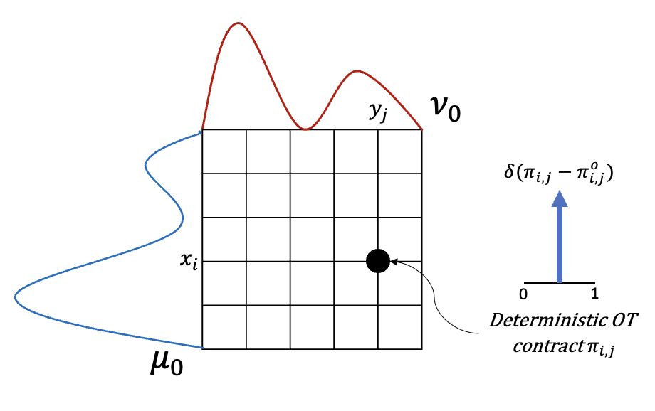
(a) In the base OT setting, the contract $\pi_{ij}$ is a crisp, deterministic object. The contract’s distribution, $\delta(\pi_{ij}-\pi^{o}_{ij})$, is singular at $\pi^{o}_{ij}$, where $\pi^{o}$ denotes the OT plan (8).

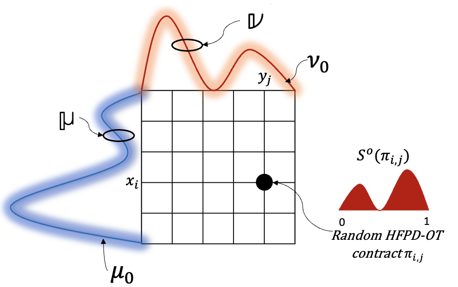
(b) Opposed to the base OT, HFPD-OT regards ($\mu$, $\nu$) and the contracts $\pi_{ij}$ as stochastic processes endowed with their own distributions. $\mathsf{S}^{o}(\pi_{ij})$ is the marginal distribution of $\pi_{ij}$, with support in [0, 1].

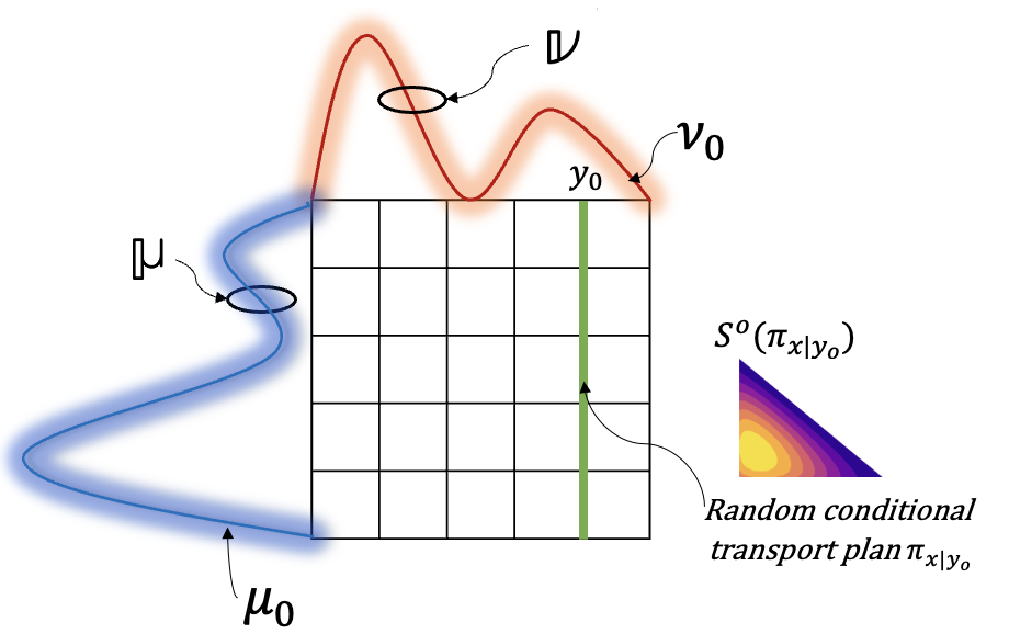
(c) Similarly, for a fixed $y_{0}\in\mathbb{\Omega}_{Y}$, the conditional distribution $\pi_{x|y_{0}}$ is a regarded in HFPD-OT as a stochastic process, equipped with its own distribution $\mathsf{S}^{o}(\pi_{x|y_{0}})$.

Figure 1: A schematic illustrating the main difference between base OT (left) and HFPD-OT (middle and right). For the sake of illustration, we consider the finite dimensional setting (which shall be reviewed in full detail in Section 4). In HFPD-OT, all quantities of interest are modelled as stochastic processes. This is the case for single contracts $\pi_{ij}$, marginal and conditional distributions. A contract refers here to the normalized quantity of resources (information, assets, stock, etc.) transferred from node $x_{i}\in\mathbb{\Omega}_{X}$ to node $y_{j}\in\mathbb{\Omega}_{Y}$. Studying these distributions conveys far more insights about the transport problem than a single and deterministic quantity.

3 Hierarchical Fully Probabilistic Design for (Optimal) Transport: FPD-OT

The classical OT setting contemplates the transport plan as a purely deterministic object and frames the OT problem solely from an optimization perspective (Figure 1(a)). More precisely, FPD-OT [Quinn et al., 2024], which is a generalization of the classical EOT problem [Cuturi, 2013], is built upon the following optimization problem:

$$\pi^{o}_{\mathsf{OT},\epsilon,\phi}(x,y|K)=\operatorname*{argmin}_{\pi\in\mathbb{\Pi}(\mu_{0},\nu_{0})}\mathsf{D}_{\mathsf{KL}}(\pi(x,y)||\pi_{\mathsf{I}}(x,y))$$ (6)

where the base ideal design $\pi_{\mathsf{I}}$ with support in $\mathbb{\Omega}_{X}\times\mathbb{\Omega}_{Y}$ is defined as the following extended Gibbs kernel:

$$\pi_{\mathsf{I}}(x,y|K)\propto\exp\Bigl{(}\frac{-\mathsf{C}(x,y)}{\epsilon}\Bigr{)}\phi(x,y)$$ (7)

$\mathsf{C}:\mathbb{\Omega}_{X}\times\mathbb{\Omega}_{Y}\rightarrow\mathbbm{R}^{+}$ denotes a continuous cost function, $\epsilon>0$ is a smoothness parameter and $\phi$ is a fixed distribution, which may be used to encode additional structural preferences in the design of the OT plan. $K$ (Section 2.2) denotes the deterministic, domain-specific knowledge constraints, consisting of external or side-information gathered from the environment, and any other prior knowledge related to the problem being modelled. In the base OT setting, we impose these knowledge constraints in the form of deterministic marginal constraints $\mathbb{\Pi}(\mu_{0},\nu_{0})$ (2). Importantly, when $\phi$ is instantiated as the uniform distribution, $\mathcal{U}$, with support in $\mathbb{\Omega}_{X}\times\mathbb{\Omega}_{Y}$, the resulting classical entropic OT solution converges in the $\Gamma$-sense to the Monge-Kantorovitch solution [Carlier et al., 2017]:

$$\pi^{o}_{\mathsf{OT},\epsilon,\mathcal{U}}(x,y|K)\xrightarrow[]{\epsilon\rightarrow 0}\pi^{o}_{\mathsf{OT}}(x,y|K)\equiv\operatorname*{argmin}_{\pi\in\mathbb{\Pi}(\mu_{0},\nu_{0})}\int_{\mathbb{\Omega}_{X}\times\mathbb{\Omega}_{Y}}\mathsf{C(x,y)}\pi(x,y)d\lambda(x,y)$$ (8)

In the sequel, we will refer to the OT solution simply by $\pi^{o}$ and won’t distinguish between EOT and OT solutions, unless required by the context.

Opposed to the aforementioned paradigm, HFPD-OT no longer regards $\pi$ as a deterministic object. The transport plan is modelled as a stochastic process in the space of random decision strategies, furnished with its own hierarchical model (Figure 1(b)). In the following Section, we introduce the setup of HFPD-OT and state the main result characterising formally the optimal hyperprior (1).

3.1 HFPD-OT formulation

To accommodate the new HFPD-OT setting, the mathematical problem is stated in an extended, hierarchical measurable space: $(\mathbb{\Omega}_{\mathsf{H}},\mathcal{F}_{\mathbb{\Omega}_{\mathsf{H}}})$, where $\mathbb{\Omega}_{\mathsf{H}}\equiv\mathbb{\mathbb{\Omega}}_{X}\times\mathbb{\mathbb{\Omega}}_{Y}\times\mathbbm{P}(\mathbb{\mathbb{\Omega}}_{X}\times\mathbb{\mathbb{\Omega}}_{Y})$ and $\mathcal{F}_{\mathbb{\Omega}_{\mathsf{H}}}$ is the $\sigma$-algebra of measurable sets of $\mathbb{\Omega}_{\mathsf{H}}$. Furthermore, $\mathbb{\mathbb{\Omega}}_{X}$ and $\mathbb{\mathbb{\Omega}}_{Y}$ are now assumed to be compact sets of an infinite dimensional topological space. In this new setting, $\pi\in\mathbbm{P}(\mathbb{\Omega}_{X}\times\mathbb{\Omega}_{Y})$ is a random process endowed with its own distribution, called the hyperprior and denoted by $\mathsf{S}(\pi|K)$. The notation $\pi\sim\mathsf{S}(\pi|K)$ means that $\pi$ is a realization of the hyperprior $\mathsf{S}(\pi|K)$ given the knowledge constraints, $K$ (which will be specified below). Moreover, let $\mathcal{L}(\pi)$ denote the reference measure in this extended probability space. In the discrete case — when $\mathbbm{P}(\mathbb{\Omega}_{X}\times\mathbb{\Omega}_{Y})$ reduces to the probability simplex — $\mathcal{L}(\pi)$ defaults to the Lebesgue measure, $\lambda$. As in the base OT setting, we assume that $\mathsf{S}(\pi|K)$ is absolutely continuous w.r.t the reference measure $\mathcal{L}(\pi)$ and we overload $\mathsf{S}(\pi|K)$ to designate its Radon-Nikodym derivative w.r.t $\mathcal{L}(\pi)$.

Let $\mathbb{M}_{\mathsf{H}}$ be the set of joint hierarchical Bayesian models with support in $\mathbb{\Omega}_{\mathsf{H}}$. The joint hierarchical Bayesian model $\mathsf{M}(x,y,\pi|\mathsf{S},K)\in\mathbb{M}_{\mathsf{H}}$ — our new variational object — reads as follows:

$$\begin{split}\mathsf{M}(x,y,\pi|\mathsf{S},K)&=\mathsf{M}(x,y|\pi,\mathsf{S},K)\mathsf{M}(\pi|\mathsf{S},K)\\ &=\pi(x,y|K)\mathsf{S}(\pi|K)\end{split}$$ (9)

(9) is a direct consequence of the conditional independence structure intrinsic to hierarchical modelling (Figure 2), and the fundamental definitions of $\pi$ and $\mathsf{S}$.

[Expected transport plan] The random transport plan, $\pi\sim\mathsf{S}(\pi|K)$ (9), has the expected value,

$$\hat{\pi}_{\mathsf{S}}(x,y|K)\equiv\mathsf{E}_{\mathsf{S}}[\pi]\equiv\int_{\mathbb{P}(\mathbb{\Omega}_{X}\times\mathbb{\Omega}_{Y})}\pi(x,y|K)\mathsf{S}(\pi|K)d\mathcal{L}(\pi).$$ (10)

Hence, the marginal model of $(x,y)$—and, therefore, the base-level transport plan induced by $\mathsf{S}$—is $\hat{\pi}_{\mathsf{S}}$ (10), as may be seen by integrating both sides of (9) over $\pi\in\mathbbm{P}(\mathbb{\mathbb{\Omega}}_{X}\times\mathbb{\mathbb{\Omega}}_{Y})$:

$$\pi(x,y|K)=\hat{\pi}_{\mathsf{S}}(x,y|K).$$ (11)

This is a necessary condition for consistent hierarchical Bayesian modelling, and arises because of the deterministic mapping, $(x,y)\rightarrow\pi(x,y)$, imposed by any realization of $\pi\sim\mathsf{S}(\pi|K)$.

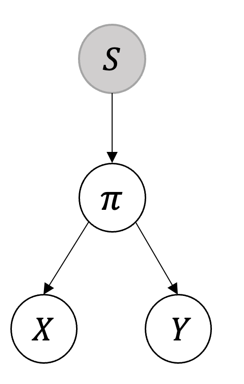
Figure 2: The conditional independence map associated with HFPD-OT. Shaded nodes are observed. The arrows indicate the causal structure, where an arrow from one variable to a second indicates that the first variable causes the second.

From the foregoing, it is evident that the problem of hierarchical transport model design is one of optimization of deterministic $\mathsf{S}\in{\mathbb{S}}(\mathbbm{P}(\mathbb{\mathbb{\Omega}}_{X}\times\mathbb{\mathbb{\Omega}}_{Y}))$, noting that $\mathsf{S}$ appears as a condition in (9). The challenge in designing the optimal hierarchical model over the set of transport plans in (9) is to optimally process the stochastic knowledge constraints imposed by the uncertain environment while being close to an ideal design $\mathsf{M}_{\mathsf{I}}$, which is used by the modeller to encode additional inductive biases and preferences in the HFPD-OT problem.
The generalized Bayesian inference framework considered here for the purpose of designing the optimal hierarchical model is Fully Probabilistic Design (FPD), introduced in [Kárný and Kroupa, 2012] and extended later to the hierarchical setting in [Quinn et al., 2016]. Generalized Bayesian inference (GBI) is a set of techniques that extend the classical Bayesian inference method by updating the prior belief distribution using a loss function rather than the traditional likelihood function. Under incomplete model specification, the latter may indeed not exist [Bissiri et al., 2016]. However, FPD differs from other GBI techniques in two ways. First, FPD relies on the concept of ideal design in place of a prior, and let the modeller elicit their personal preferences in the design process through an ideal, and usually unattainable, distribution $\mathsf{M}_{\mathsf{I}}(x,y,\pi)\in{\mathbb{M}}_{\mathsf{H}}^{c}\equiv\mathbb{M}\smallsetminus\mathbb{M}_{\mathsf{H}}$ (Figure 3). More precisely, let’s assume that the ideal design factorises as follows:

$$\mathsf{M}_{\mathsf{I}}(x,y,\pi)\equiv\pi_{\mathsf{I}}(x,y)\mathsf{S}_{\mathsf{I}}(\pi)$$ (12)

In other words, the joint ideal design $\mathsf{M}_{\mathsf{I}}(x,y,\pi)$ is the base ideal design $\pi_{\mathsf{I}}$, modulated by the hierarchical ideal design $\mathsf{S}_{\mathsf{I}}(\pi)$. $\mathsf{M}_{\mathsf{I}}(x,y,\pi)$ is unattainable because $\pi_{\mathsf{I}}$ and $\mathsf{S}_{\mathsf{I}}(\pi)$ are statistically independent and as such, they may be conflicting in the following sense:

$$\mathsf{E}_{\mathsf{S}_{\mathsf{I}}}(\pi)\neq\pi_{\mathsf{I}}(x,y)$$ (13)

This is in itself not a design error, for ideal designs are purely subjective objects used to encode the modeller’s preferences. The use of the concept of ideal design and preferences, in place of the usual prior, makes FPD an instance of Savage’s subjective expected utility elicitation [Savage, 1971]. The second difference that sets FPD apart from other GBI techniques relates to the fact that FPD does not proceed by updating the prior belief to a posterior distribution but is rather concerned with ranking and selecting the most appropriate random decision strategy, given a knowledge constraint set $K$. This selection is done by means of the KL divergence [Bernardo, 1979], [Shore and Johnson, 1980], and the corresponding optimization problem reads:

$$(P):\;\;\;\;\;\mathsf{M}^{o}\in\operatorname*{argmin}_{\mathsf{M}\in\mathbb{M}_{\mathsf{H}}}\left\{\mathsf{D}_{\mathsf{KL}}\bigl{(}\mathsf{M}(x,y,\pi|K)||\mathsf{M}_{\mathsf{I}}(x,y,\pi)\bigr{)}\right\}$$ (14)

subject to:

$$\mathsf{E}_{\mathsf{S}}(\mathsf{D}_{\mathsf{KL}}(\mu||\mu_{0}))\leq\eta$$ (15)

$$\mathsf{E}_{\mathsf{S}}(\mathsf{D}_{\mathsf{KL}}(\nu||\nu_{0}))\leq\zeta$$

We note the following:

1. Since the $\mathsf{D}_{\mathsf{KL}}\bigl{(}\cdot||\mathsf{M}_{\mathsf{I}}\bigr{)}$ is continuous, the space of joint hierarchical Bayesian distributions $\mathbb{M}_{\mathsf{H}}$ is compact in the weak-* topology (see Appendix 7) and the constraint set is nonempty (we can take for instance $\mathsf{S}=\delta_{\mu_{0}\otimes\nu_{0}}$), then the minimum is attained.

2. Moreover, the optimal joint hierarchical model $\mathsf{M}^{o}$ is unique up to a set of measure 0.

The ideal design $\mathsf{M}_{\mathsf{I}}$ enters the KL divergence as the second fixed argument against which all feasible Bayesian hierarchical models are ranked. Importantly, note that the marginals in (14) are no longer modelled as deterministic, crisp objects. This assumption is now relaxed, allowing for the modeller to express their uncertainty by viewing the marginals as random realizations of some underlying stochastic process. In particular, we describe this uncertainty in the form of moment constraints: the random marginals belong to uncertainty sets in the form of Kullback-Leibler balls, centred on $\mu_{0}\in\mathbbm{P}(\mathbb{\Omega}_{X})$ and $\nu_{0}\in\mathbbm{P}(\mathbb{\Omega}_{Y})$. The new knowledge-constrained set of consistent hierarchical Bayesian models — denoted by $\mathbb{M}_{K}\subseteq\mathbb{M}_{\mathsf{H}}$ — is augmented with the following linear moment constraints over the marginals:

$$\begin{split}\mathbb{M}_{K}\equiv\Bigl{\{}\mathsf{M}(x,y,\pi|K)\;|\;\mathsf{M}(x,y,\pi|K)\in\mathbb{M}_{\mathsf{H}}\;,\;\mu\in\bbmu\;\text{and}\;\nu\in\bbnu\Bigr{\}}\end{split}$$ (16)

with the sets $\bbmu$ and $\bbnu$ defined as follows (Figure 1(b)):

$$\bbmu\equiv\{\mu\in\mathbb{P}(\mathbb{\Omega}_{X})\;|\;\mathsf{E}_{\mathsf{S}}\left[\mathsf{D}_{\mathsf{KL}}(\mu||\mu_{0})\right]\leq\eta\}$$ (17)

$$\bbnu\equiv\{\nu\in\mathbb{P}(\mathbb{\Omega}_{Y})\;|\;\mathsf{E}_{\mathsf{S}}\left[\mathsf{D}_{\mathsf{KL}}(\nu||\nu_{0})\right]\leq\zeta\}$$ (18)

where $\eta\geq 0$ and $\zeta\geq 0$ are prior-elicited KL radii, that express the degree of uncertainty the modeller is placing over the marginals.

As we shall see in the sequel, the interaction between base and hierarchical ideals on one hand and the knowledge constraints on the other, gives rise to the Gibbs form of the hyperprior in (1). We shall now state the main result of this Section.

Let (P) be the HFPD-OT Primal problem, defined in (14).

1. (P) is equivalent to the following optimization problem over the set of hierarchical Bayesian models $\mathbb{M}_{\mathsf{H}}$ (16):

   $$(P):\;\;\;\;\;\mathsf{M}^{o}(x,y,\pi)\in\operatorname*{argmin}_{\mathsf{M}\in\mathbb{M}_{\mathsf{H}}}\left\{\mathsf{D}_{\mathsf{KL}}\bigl{(}\mathsf{M}(x,y,\pi|K)||\hat{\pi}_{\tilde{\mathsf{S}}}(x,y)\tilde{\mathsf{S}}(\pi|K)\bigr{)}\right\}$$ (19)

   subject to:

   $$\left\{\begin{aligned} \mathsf{E}_{\mathsf{S}}(\mathsf{D}_{\mathsf{KL}}(\mu||\mu_{0}))\leq\eta\\ \mathsf{E}_{\mathsf{S}}(\mathsf{D}_{\mathsf{KL}}(\nu||\nu_{0}))\leq\zeta\end{aligned}\right.$$

   where:

   $$\tilde{\mathsf{S}}(\pi|K)\equiv\mathsf{S}_{\mathsf{I}}(\pi)\exp\Bigl{(}-\mathsf{D}_{\mathsf{KL}}\bigl{(}\pi(x,y)||\pi_{\mathsf{I}}(x,y)\bigr{)}\Bigr{)}$$ (20)

2. The optimal hyperprior $\mathsf{S}^{o}(\pi|K)$ reads as follows:

   $$\mathsf{S}^{o}(\pi|K)\propto\exp\left(-\lambda_{1}^{o}{\mathsf{D}_{\mathsf{KL}}}(\mu||\mu_{0})\right)\tilde{\mathsf{S}}(\pi|K)\exp\left(-\lambda_{2}^{o}{\mathsf{D}_{\mathsf{KL}}}(\nu||\nu_{0})\right)\;\;\mathcal{L}\text{-a.e.}$$ (21)

3. The Dual program associated with the primal $(P)$ (19) reads:

   $$\begin{split}(D):\;\;\;\;\sup_{\boldsymbol{\lambda}\succeq 0}\left\{\log\left(\mathsf{N}(\boldsymbol{\lambda})\right)-\boldsymbol{\lambda}^{\intercal}\boldsymbol{\theta}\right\}\end{split}$$ (22)

   where:

   $$\mathsf{N}(\boldsymbol{\lambda})\equiv\left(\int_{\mathbbm{P}(\mathbb{\Omega}_{X}\times\mathbb{\Omega}_{Y})}\tilde{\mathsf{S}}(\pi|K)\exp\left(-<\boldsymbol{\lambda},\mathsf{R}(\pi)>-1\right)d\mathcal{L}(\pi)\right)^{-1}$$ (23)

   and: $\boldsymbol{\lambda}$ $\equiv$ $\begin{bmatrix}\lambda_{1}\\ \lambda_{2}\end{bmatrix}$, $\boldsymbol{\theta}\equiv\begin{bmatrix}\eta\\ \zeta\end{bmatrix}$, $\mathsf{R}(\pi)$ $\equiv$ $\begin{bmatrix}\mathsf{D}_{\mathsf{KL}}(\mu||\mu_{0})\\ \mathsf{D}_{\mathsf{KL}}(\nu||\nu_{0})\end{bmatrix}$
   
   Moreover, strong duality holds, i.e. the optimal Kantorovitch potentials, $\boldsymbol{\lambda}^{o}$ in (21), are the solution of the dual problem (22),

   $$\boldsymbol{\lambda}^{o}\equiv\operatorname*{argmax}_{\boldsymbol{\lambda}\succeq 0}\left\{\log\left(\mathsf{N}(\boldsymbol{\lambda})\right)-\boldsymbol{\lambda}^{\intercal}\boldsymbol{\theta}\right\},$$ (24)

   and the maximum of the dual problem is attained: $\min_{\mathsf{M}}(P)=\max_{\boldsymbol{\lambda}}(D)$.

Proof method.

Results (1) and (2) of the Theorem can be proved using basic algebraic manipulations. However, we opt here for a derivation based on information processing arguments, so as to gain more intuition about the design of the hyperprior in the hierarchical setting.

Given the factorized joint ideal design in (12), the optimal hyperprior $\mathsf{S}^{o}(\pi|K)$ emerges via two sequential knowledge-processing steps (Figure 3), addressed in the first two of the following items:

1. Adapting the ideal design and processing the hyperprior without knowledge constraints $K$. The purpose of this first step is to guide the optimization problem $(P)$ in (14) from a possibly inconsistent ideal, $\mathsf{M}_{\mathsf{I}}$ (13), to a new consistent target (step 1 in Figure 3). The adapted hyperprior, $\tilde{\mathsf{S}}$ (20), expresses the best compromize between possibly conflicting ideals. It involves the Gibbs-type modulation of the hierarchical ideal design $\mathsf{S}_{\mathsf{I}}$ via a term that depends on the ideal base-level design $\pi_{\mathsf{I}}$ (Theorem 1 in [Quinn et al., 2016]). The optimal hierarchical model $\tilde{\mathsf{M}}\in\mathbb{M}_{\mathsf{H}}$ is a boundary point in the convex set $\mathbb{M}_{\mathsf{H}}$ and is inferred from (9) as follows:

   $$\tilde{\mathsf{M}}(x,y,\pi|K)=\hat{\pi}_{\tilde{\mathsf{S}}}(x,y|K)\tilde{\mathsf{S}}(\pi|K)$$ (25)

   where $\hat{\pi}_{\tilde{\mathsf{S}}}$ is the expected transport plan w.r.t $\tilde{\mathsf{S}}$ and follows from (10).

2. Processing the two marginal constraints specified in the knowledge set $K$. This step leads to the new optimization problem stated in (19), which results in the optimal hyperprior (21) (Theorem 3 in [Quinn et al., 2016]). Each of the marginal constraints induces a MaxEnt Gibbs term that modulates the hyperprior obtained in Step 1. And the resulting optimal hierarchical model $\mathsf{M}^{o}\in\mathbb{M}_{K}\subseteq\mathbb{M}_{\mathsf{H}}$ — which is also a boundary point in the convex set $\mathbb{M}_{K}$ — reads as follows:

   $$\mathsf{M}^{o}(x,y,\pi|K)=\hat{\pi}_{\mathsf{S}^{o}}(x,y|K)\mathsf{S}^{o}(\pi|K)$$ (26)

   where $\hat{\pi}_{\mathsf{S}^{o}}$ follows similarly from (10).

3. It remains to prove the strong duality result and formally characterize the Kantorovitch potentials in (22). The details of this proof are provided in Appendix 7. There, we prove strong duality in the infinite dimensional case by relying on the classical Fenchel-Rockafellar duality theorem [Rockafellar, 1967], [Villani, 2008]. More precisely, we demonstrate that the conditions required by the theorem are satisfied in the hierarchical Bayesian setting of HFPD-OT, and we derive the dual problem $(D)$.

∎

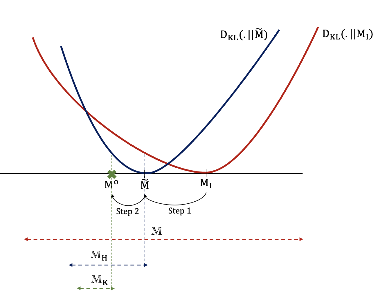
Figure 3: A sequential information-processing view of the optimal hierarchical model $\mathsf{M}^{o}\equiv\hat{\pi}_{{\mathsf{S}}^{o}}\mathsf{S}^{o}$ (26). First, the inductive biases expressed via the hierarchical ideal model, $\mathsf{M}_{\mathsf{I}}\in{\mathbb{M}}_{\mathsf{H}}^{c}$ (12), are processed to yield a new optimization problem over a constrained set $\mathbb{M}_{\mathsf{H}}$, whose solution, $\tilde{\mathsf{M}}$ (25), is on the boundary of $\mathbb{M}_{\mathsf{H}}$. Second, the knowledge constraints, $K$, are processed, further reducing the feasible set to the subset, $\mathbb{M}_{K}$ (16). The optimal hierarchical model is $\mathsf{M}^{o}$ (on the boundary of $\mathbb{M}_{K}$), s.t. $\pi\sim\mathsf{S}^{o}$ (21).

By sampling random realizations from our optimal hyperprior, we can design randomized and diverse transport policies in lieu of an immutable and fixed OT plan. This randomization principle is depicted in Figure 4. More precisely, the design of the optimal hyperprior over the space of transport plans is a twofold process:

1. The knowledge constraints $K$ are processed to yield the optimal hyperprior $\eqref{eq:hyperprior}$. This mainly requires conditioning the Kantorovitch potentials on the uncertainty radii $(\eta,\zeta)$ (Figure 4(a)).

2. Once the optimal hyperprior available, random transport strategies can be sampled and used in subsequent transport problems in place of a crisp OT plan. Importantly, having access to a generative model over the space of transport plans provides us with all the tools to reason and measure the intrinsic uncertainty to the transport problem (Figure 4(b)). The expected transport $\hat{\pi}_{\mathsf{S}^{o}}$ plan is obtained from (10).

Remark 1.

The Kantorovitch potentials $\lambda_{1}=\lambda_{1}(\eta,\zeta)$ and $\lambda_{2}=\lambda_{2}(\eta,\zeta)$ express the degree of uncertainty in the input data — i.e. the marginals. Depending on their values, they give rise to two interesting extremal modalities, that vary from high uncertainty to perfect characterization of the marginals:

• If $\eta\rightarrow\infty$ and $\zeta\rightarrow\infty$, it is straightforward from (22) that the solution of the dual is achieved when $\boldsymbol{\lambda}^{o}=\boldsymbol{0}$. This is also a direct consequence of complementary slackness. It follows that:

  $$\mathsf{S}^{o}(\pi|K)\xrightarrow[]{\eta\to\infty,\;\zeta\to\infty}\tilde{\mathsf{S}}(\pi|K)$$ (27)

  In other words, when the uncertainty around the marginals is unbounded, the optimal hyperprior is mainly characterized by the product of the hierarchical ideal design and a Gibbsian term that depends on $\pi_{\mathsf{I}}$.

• If $\eta\rightarrow 0$ and $\zeta\rightarrow 0$, the uncertainty in the marginals vanishes and learning is maximal, leading to: $\mu\rightarrow\mu_{0}$ and $\nu\rightarrow\nu_{0}$, or equivalently: $\pi\rightarrow\tilde{\pi}\in\mathbb{\Pi}(\mu_{0},\nu_{0})$. It follows from the dual (22) that the maximum is attained when: $\boldsymbol{\lambda}^{o}\rightarrow\infty$ and we have in the limit:

  $$\mathsf{S}^{o}(\pi|K)\xrightarrow[]{\eta\to 0,\;\zeta\to 0}\tilde{\mathsf{S}}(\pi|K)\delta_{\pi}(\mathbb{\Pi}(\mu_{0},\nu_{0}))$$ (28)

  In other words, the hyperprior degenerates to the statistical manifold with support in $\mathbb{\Pi}(\mu_{0},\nu_{0})$. This concentration behaviour is reminiscent of the Laplace-Bernstein-Von Mises convergence theorem [Borwanker et al., 1971]: under some regularity conditions, it implies the convergence of the posterior distribution to the best approximation of the data generation process, in the KLD sense.

Remark 2.

Base-level OT Let’s consider the regime of perfect specification of the marginals, i.e. $\eta\rightarrow 0$,$\zeta\rightarrow 0$. The conjugate choice of the ideal hyperprior, $\mathsf{S}_{\mathsf{I}}$, has the following Gibbs form:

$$\mathsf{S}_{\mathsf{I}}(\pi|K)\propto\exp(-\alpha\mathsf{D}_{\mathsf{KL}}(\pi(x,y)||\pi_{\mathsf{I}}(x,y)))$$ (29)

where $\alpha>0$ plays the role of the inverse of the temperature. By plugging in this expression into (28), the optimal hyperprior becomes:

$$\mathsf{S}^{o}(\pi|K)\xrightarrow[]{\eta\to 0,\;\zeta\to 0}\exp(-(\alpha+1)\mathsf{D}_{\mathsf{KL}}(\pi||\pi_{\mathsf{I}}))\delta_{\pi}(\mathbb{\Pi}(\mu_{0},\nu_{0}))$$ (30)

When $\pi_{\mathsf{I}}$ is the extended Gibbs kernel (7), where we instantiate $\phi$ as the Uniform distribution with support in $\mathbb{\Omega}_{X}\times\mathbb{\Omega}_{Y}$, the minimum of $\mathsf{D}_{\mathsf{KL}}(\pi||\pi_{\mathsf{I}})$ in (30) is exactly achieved at the EOT solution (8):

$$\pi^{o}(x,y|K)=\operatorname*{argmin}_{\pi\in\mathbb{\Pi}(\mu_{0},\nu_{0})}\mathsf{D}_{\mathsf{KL}}(\pi(x,y)||\pi_{\mathsf{I}}(x,y))$$ (31)

The latter can be recovered when $\alpha\rightarrow\infty$, for example by simulated annealing [Delahaye et al., 2019]:

$$\mathsf{S}^{o}(\pi|K)\xrightarrow[]{\eta\to 0,\;\zeta\to 0,\alpha\to\infty}\delta_{\pi^{o}}$$ (32)

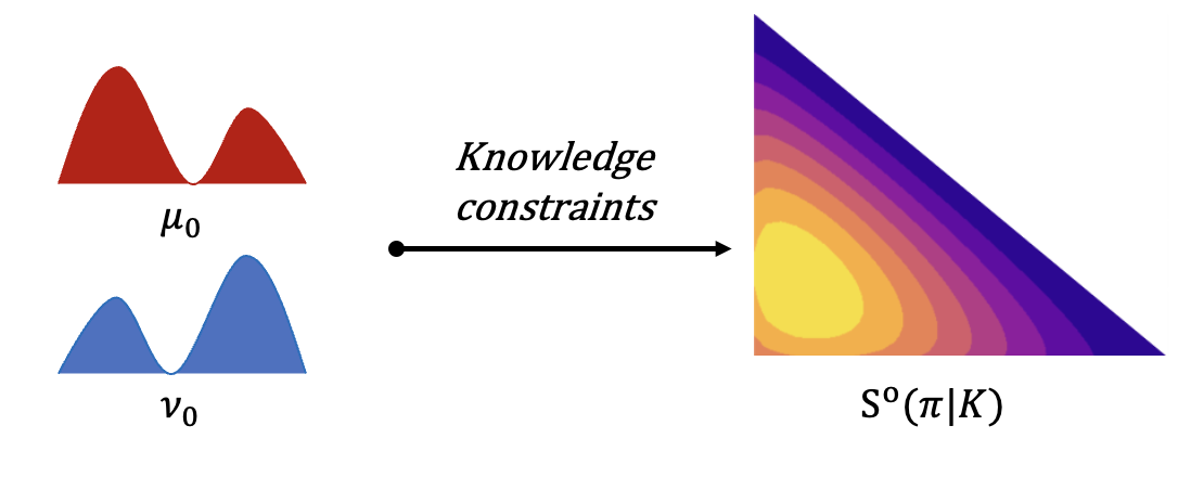
(a) As a first step, the optimal hyperprior $\mathsf{S}^{o}(\pi|K)$ is computed, by mainly processing the optimal Kantorovitch potentials (knowledge constraints).

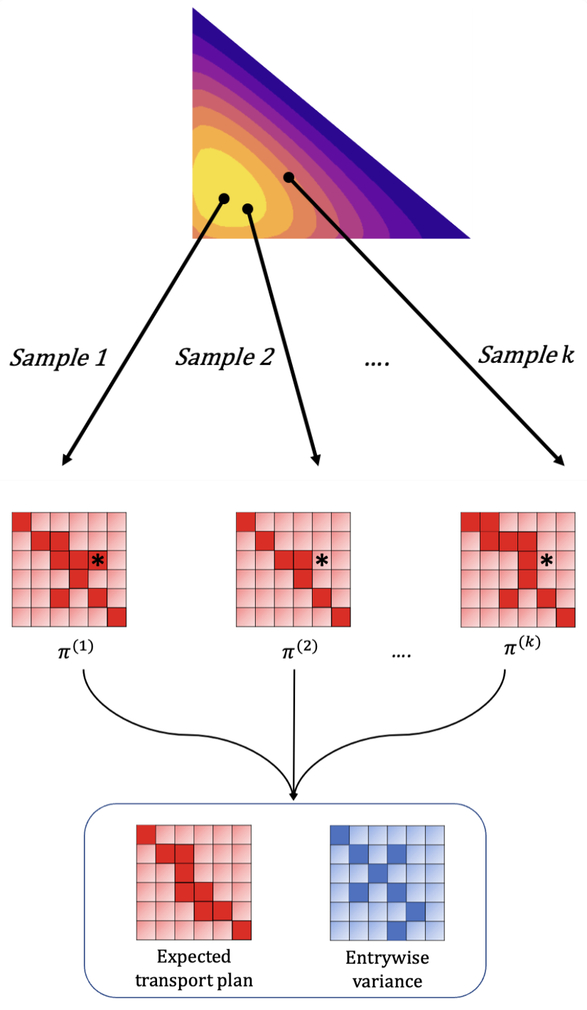
(b) Once available, the optimal hyperprior $\mathsf{S}^{o}(\pi|K)$ can be used to sample random realizations of transport plans. These samples can be leveraged to construct two crucially important objects: 1. The expected transport plan, which can be used in downstream transport tasks, in lieu of the OT plan (bottom left) and 2. measures of uncertainty in the form of entrywize variances or other summary statistics (bottom right). The asterisk (*) highlights an example of a contract that experiences diversified transport policies, enabled by randomized HFPD-OT.

Figure 4: Schematic illustrating the 2-step principle underlying HFPD-OT. $\mathsf{S}^{o}(\pi|K)$ is a generative model, i.e. a probability density over random transports plans $\pi$. Different realizations of the transport plan $\pi$ can be sampled from $\mathsf{S}^{o}(\pi|K)$. These samples can then be used to construct an expected transport plan for downstream transport problems. In addition, HFPD-OT allows for a principled analysis of uncertainty in the transport problem.

4 The parametric HFPD-OT hyperprior

As already noted, no special assumptions have been made in respect of the hierarchical transport model (9), and so (21) is the HFPD-OT hyperprior for the nonparametric (transport) process, $\pi\in\mathbbm{P}(\mathbb{\Omega}_{X}\times\mathbb{\Omega}_{Y})$. The finite case—i.e. $\#(\mathbb{\Omega}_{X}\times\mathbb{\Omega}_{Y})<\infty$—induces the parametric setting of HFPD-OT, with $\pi$ defined in the usual way w.r.t. counting measure, and $\mathsf{S}^{o}(\pi)$ defined on a $K$-constrained subset (15) of the simplex. This allows us to easily visualize key properties of $\mathsf{S}^{o}$ in a low dimensional setting, and, importantly, to develop algorithms for computing random draws (Figure 4(b)), $\pi^{(k)}\sim\mathsf{S}^{o}$, from the HFPD-OT parametric hyperprior (21), via approximation of the Kantorovitch potentials (24).

4.1 Descriptive analysis of the parametric HFPD-OT hyperprior, $\mathsf{S}^{o}$

In the finite, parametric case—which we will pursue in the rest of this paper—$\mathbb{\Omega}_{X}\equiv\{x_{1},\ldots,x_{i},\ldots,x_{m}\}$ and $\mathbb{\Omega}_{Y}\equiv\{y_{1},\ldots,x_{j},\ldots,x_{n}\}$, with $2\leq m<\infty$ and $2\leq n<\infty$. We refer to $\mathbb{\Omega}_{X}$ and $\mathbb{\Omega}_{Y}$ as the sets of source nodes and target nodes, respectively. Then, the base-level distributions are uncertain multinomials, with densities $\mu=\sum_{i=1}^{m}\mu_{i}\delta_{x_{i}}$, $\nu=\sum_{j=1}^{n}\nu_{j}\delta_{y_{j}}$ and $\pi=\sum_{j=1}^{n}\sum_{i=1}^{m}\pi_{i,j}\delta_{x_{i},y_{j}}$. The associated pmfs are structured as vector-matrix objects, and also denoted by the same symbols: $\mu\in\Delta_{m-1}$, $\nu\in\Delta_{n-1}$ and $\pi\in\Delta_{mn-1}$. Without loss of generality, we consider the following class of conjugate hierarchical ideal designs, parameterized by fixed ${\boldsymbol{\lambda}}_{\mathsf{I}}\succeq 0$:

$$\mathsf{S}_{\mathsf{I}}(\pi|K)\propto\prod_{i=1}^{m}\Bigl{(}\frac{\mu_{i}}{\mu_{0,i}}\Bigr{)}^{-\lambda_{\mathsf{I},1}\mu_{i}}\prod_{j=1}^{n}\Bigl{(}\frac{\nu_{j}}{\nu_{0,j}}\Bigr{)}^{-\lambda_{\mathsf{I},2}\nu_{j}}$$ (33)

To align with the FPD-OT setting [Quinn et al., 2024], the base ideal design, $\pi_{\mathsf{I}}$, takes the form of the extended Gibbs kernel (7). We further specialize $\phi$ to the uniform case, $\phi\equiv{\mathcal{U}}$, yielding the following form of the parametric hyperprior: [Hyperprior for the parametric transport plan] The transport hyperprior in the case of a domain of finite cardinality, $m\times n$, has parameters $(\lambda_{1}^{o},\lambda_{2}^{o},\lambda_{\mathsf{I},1},\lambda_{\mathsf{I},2},\mu_{0},\nu_{0},\pi_{\mathsf{I}})$, and support on the probability simplex $\Delta_{m\times n-1}$. It is absolutely continuous w.r.t the Lebesgue measure and its density reads:

$$\mathsf{S}^{o}(\pi|K)\propto\prod_{i=1}^{m}\prod_{j=1}^{n}\Bigl{(}\frac{\mu_{i}}{\mu_{0,i}}\Bigr{)}^{-(\lambda_{\mathsf{I},1}+\lambda_{1}^{o})\mu_{i}}\Bigl{(}\frac{\nu_{j}}{\nu_{0,j}}\Bigr{)}^{-(\lambda_{\mathsf{I},2}+\lambda_{2}^{o})\nu_{j}}\Bigl{(}\frac{\pi_{\mathsf{I},i,j}}{\pi_{i,j}}\Bigr{)}^{\pi_{i,j}}\;\;\lambda\text{-a.e.}$$ (34)

with the ideal design having the following Gibbs form:

$$\pi_{\mathsf{I},i,j}\propto\exp\Bigl{(}-\frac{\mathsf{C}(x_{i},y_{j})}{\epsilon}\Bigr{)}$$

The number of prior parameters, encoding $K$ in (34), is $(m+1)\times(n+1)$. This confers the HFPD-OT hyperprior design with far more expressivity (i.e. degrees-of-freedom (dofs)) than default distributions on the probability simplex. For instance, a Dirichlet distribution of $\pi$ in this finite setting has $m+n+1$ fewer dofs.

Remark 3 (Inference with the HFPD-OT Hyperprior, $\mathsf{S}^{o}$).

The normalizing constant of the HFPD-OT hyperprior (34) is not available in closed form. A full study of its numerical approximation is beyond the scope of this paper.

The marginal distribution of $\pi_{1:k,1:l}\in\Delta_{k\times l-1}$, being the sub-matrix of $\pi$ associated with the contracts, $\pi_{ij}$, $1\leq i\leq k<m$ and $1\leq j\leq l<n$, is

$$\mathsf{S}(\pi_{1:k,1:l}|K)=\int_{(1-w_{kl})\Delta_{mn-kl-1}}\mathsf{S}(\pi|K)d\pi_{\backslash(1:k,1:l)},$$ (35)

where $w_{kl}\equiv\sum_{j=1}^{l}\sum_{i=1}^{k}\pi_{ij}$, and $\pi_{\backslash(1:k,1:l})$ denotes the complement of $\pi_{1:k,1:l}$ in $\pi$. As a special case, the marginal distribution on $(0,1)$, associated with the $(k,l)$th random contract, i.e. the contract between the $k$th source node and the $l$th target node, is

$$\mathsf{S}(\pi_{kl}|K)=\int_{(1-\pi_{kl})\Delta_{mn-2}}\mathsf{S}(\pi|K)d\pi_{\backslash(k,l)}.$$ (36)

Finally, the HFPD-optimal full conditional distribution of the $(k,l)$th contract—having fixed all the others at specific probabilities—is

$$\mathsf{S}^{o}(\pi_{k,l}|\pi_{\backslash(k,l)},K)\propto\mathsf{S}^{o}(\pi|K)\;\chi_{(0,1-c_{kl})}(\pi_{kl}),$$ (37)

where $c_{kl}\equiv\underbrace{\sum_{j=1}^{n}\sum_{i=1}^{m}}_{(i,j)\notin\{(k,l),(m,n)\}}\pi_{i,j}$, and $\chi$ denotes the standard Heaviside indicator of the indicated interval.

To gain further intuition about the parametric hyperprior $\eqref{eq:parametric_hyperprior}$, we explore its key properties in low dimensional setting, by mainly studying its shape and location.

Let $\mathsf{S}(\pi_{11},\pi_{12},\pi_{21}|K)$ denote the hyperprior in the probability simplex $\Delta_{3}$ (Figure 8). Its unnormalized probability density w.r.t the Lebesgue measure in $\mathbbm{R}^{3}$ reads as follows:

$$\begin{split}\mathsf{S}(\pi_{11},\pi_{12},\pi_{21}|K)\propto\Bigl{(}\frac{\pi_{11}+\pi_{12}}{\mu_{01}}\Bigr{)}^{-\lambda_{1}(\pi_{11}+\pi_{12})}\Bigl{(}\frac{1-\pi_{11}-\pi_{12}}{\mu_{02}}\Bigr{)}^{-\lambda_{1}(1-\pi_{11}-\pi_{12})}\Bigl{(}\frac{\pi_{11}+\pi_{21}}{\nu_{01}}\Bigr{)}^{-\lambda_{2}(\pi_{11}+\pi_{21})}&\\ \Bigl{(}\frac{1-\pi_{11}-\pi_{21}}{\nu_{02}}\Bigr{)}^{-\lambda_{2}(1-\pi_{11}-\pi_{21})}\Bigl{(}\frac{\pi_{11}}{\pi_{\mathsf{I},0}}\Bigr{)}^{-\pi_{11}}\Bigl{(}\frac{\pi_{12}}{\pi_{\mathsf{I},1}}\Bigr{)}^{-\pi_{12}}\Bigl{(}\frac{\pi_{21}}{\pi_{\mathsf{I},2}}\Bigr{)}^{-\pi_{21}}\Bigl{(}\frac{1-\pi_{11}-\pi_{12}-\pi_{21}}{1-\pi_{\mathsf{I},0}-\pi_{\mathsf{I},1}-\pi_{\mathsf{I},2}}\Bigr{)}^{-(1-\pi_{11}-\pi_{12}-\pi_{21})}\end{split}$$ (38)

where $(\pi_{11},\pi_{12},\pi_{21})$ satisfy: $\sum_{i=1}^{2}\sum_{j=1}^{2}\pi_{ij}=1$ with $\pi_{ij}\in[0,1]\;\forall\;(i,j)\in\{1,2\}^{2}$. The purpose of the following simulations is to study the influence of the Kantorovitch potentials $\boldsymbol{\lambda}$ and the nominal marginals $(\mu_{0},\nu_{0})$ on the shape and location of the hyperprior.

Without loss of generality, we focus primarily on the marginal distribution, which is trivially derived from (35) and reads as follows:

$$\mathsf{S}(\pi_{11},\pi_{12}|K)\propto\int_{0}^{1-\pi_{11}-\pi_{12}}\mathsf{S}(\pi_{11},\pi_{12},\pi_{21}|K)d\pi_{21}$$ (39)

This marginalisation, besides being more amenable to visual analysis in $\Delta_{2}$, is justified by many practical scenarios: we may be interested, for instance, in studying the marginal distribution of a single or a block of contracts in the transport plan (Figure 1(a)). In the following, we examine the shape and location parameters of the marginal hyperprior (39) and their connection with the knowledge constraint set $K$.

Shape parameters:

The cost matrix $\mathsf{C}$ is chosen as the Euclidean distance: $\mathsf{C}(x,y)=\begin{bmatrix}0&1\\ 1&0\end{bmatrix}$, whereas the nominal marginals are fixed to the following values: $(\mu_{0},\nu_{0})=\left\{\begin{bmatrix}0.2\\ 0.8\end{bmatrix},\begin{bmatrix}0.9\\ 0.1\end{bmatrix}\right\}$. We examine the influence of the potentials $\boldsymbol{\lambda}$ on the shape of the hyperprior, by varying their values as follows: $\boldsymbol{\lambda}\in\{0.05,10,100\}^{2}$. As discussed earlier, $\boldsymbol{\lambda}$ — through their connection with the KLD radii $(\eta,\zeta)$ — quantify the uncertainty present in the marginals and induce two notable learning modalities. The first modality takes place when $\boldsymbol{\lambda}\rightarrow\boldsymbol{0}$, and coincides with the non-specification of the marginals, hence absence of effective learning. The second modality is achieved when $\boldsymbol{\lambda}\rightarrow\infty$. This corresponds to knowledge accumulation and yields, in the limit, a perfect specification of the marginals. The empirical observations corroborate well the aforementioned concentration behaviour. In Figure 5, we show the contour plots of the marginal hyperprior $\mathsf{S}(\pi_{11},\pi_{12}|K)$ as a function of $\boldsymbol{\lambda}$. By increasing the potentials, the contours gradually concentrate on a thin statistical manifold, namely $\mathbb{\Pi}(\mu_{0},\nu_{0})$. In addition to the marginal hyperprior, we show the expected transport plan, $\hat{\pi}_{\mathsf{S}(\pi_{11},\pi_{12},\pi_{21}|K)}$, projected over its first two components ($\pi_{11}$, $\pi_{12}$) (red dot). The latter is obtained by sampling and averaging samples from the joint hyperprior: $\pi\sim\mathsf{S}(\pi_{11},\pi_{12},\pi_{21}|K)$. The blue dot, on the other hand, corresponds to the projection of the EOT plan $\pi^{o}$, computed for each pair of the nominal marginals, using Sinkhorn-Knopp iterative projections [Cuturi, 2013]. Though the expected transport plan is slightly far from the OT plan when the potentials $\boldsymbol{\lambda}$ are small, it increasingly converges towards it as the support of the marginal hyperprior contracts towards $\mathbb{\Pi}(\mu_{0},\nu_{0})$.

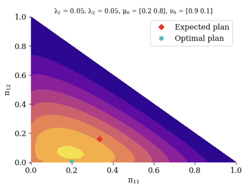
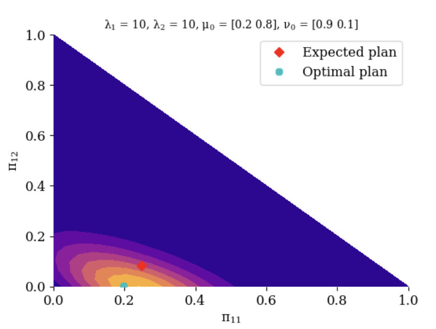
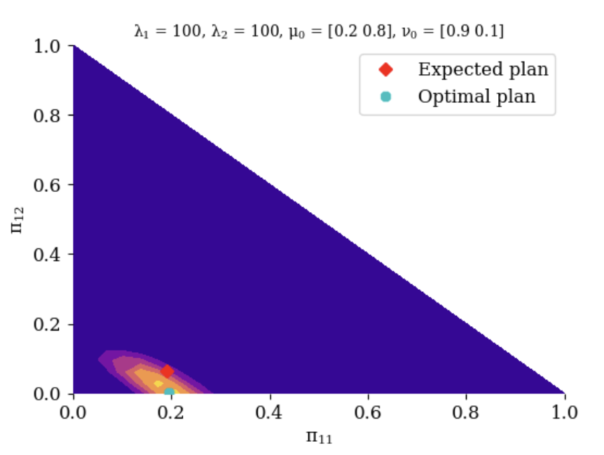
Figure 5: Contour plots of the marginal hyperprior $\mathsf{S}(\pi_{11},\pi_{12}|K)$ defined over the 2D simplex, obtained for various values of the Kantorovitch potentials and for fixed nominal marginals and base ideal design. The red point corresponds to the projection over its first two components ($\pi_{11}$, $\pi_{12}$) of the expected transport plan. We also show the projection of the EOT plan, computed between the nominal marginals (blue point).

Location parameters:

Equally important, the nominal marginals play the role of location knobs, by controlling the shift of the marginal hyperprior. To show this, let’s fix the potentials to arbitrary values: $\boldsymbol{\lambda}=(1,1)$ and vary the nominal marginals as follows:

$$(\mu_{0},\nu_{0})\in\left\{\begin{bmatrix}(0.9,0.1)\\ (0.1,0.9)\end{bmatrix}^{\intercal},\begin{bmatrix}(0.5,0.5)\\ (0.5,0.5)\end{bmatrix}^{\intercal},\begin{bmatrix}(0.1,0.9)\\ (0.9,0.1)\end{bmatrix}^{\intercal}\right\}$$ (40)

Figure 6 shows, for each pair of the nominal marginals in (40), the contour plots of the marginal hyperprior $\mathsf{S}(\pi_{11},\pi_{12}|K)$. We also plot the expected transport plan, $\hat{\pi}_{\mathsf{S}(\pi_{11},\pi_{12},\pi_{21}|K)}$, and the EOT plan $\pi^{o}$ between the nominal marginals, both of which are projected over their first two components. The location of the marginal hyperprior is clearly influenced by the nominal marginals, and specifically their relative symmetry and skewness. It is interesting to examine the evolution of the expected and optimal plans: the former is naturally attracted by the mode of the marginal hyperprior, whereas the optimal plan has initially a low probability under the marginal hyperprior but contracts eventually towards the expected plan.

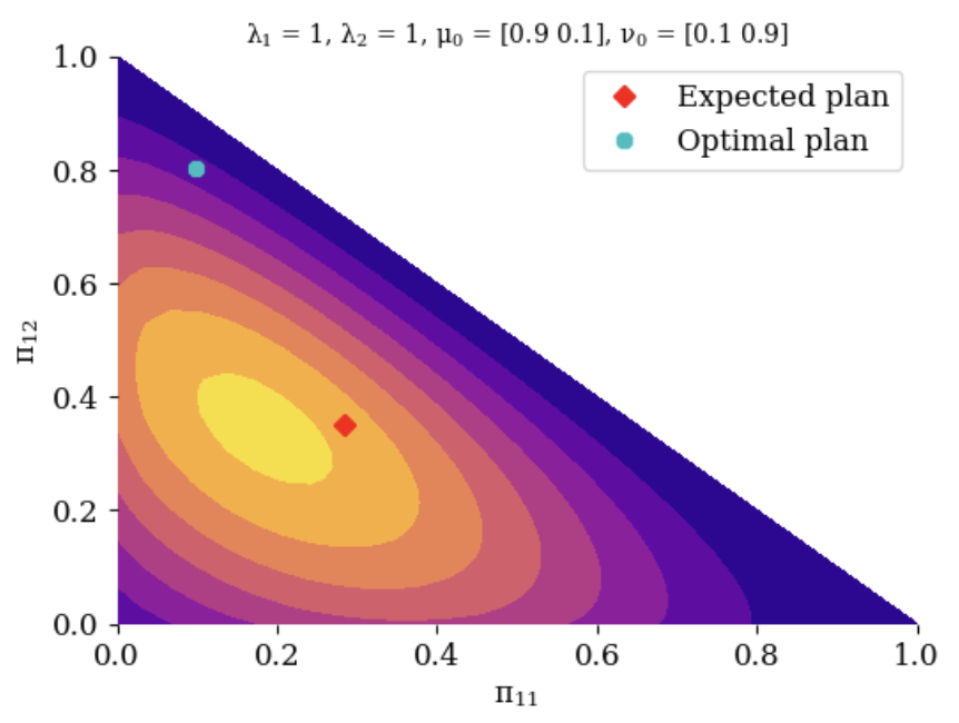
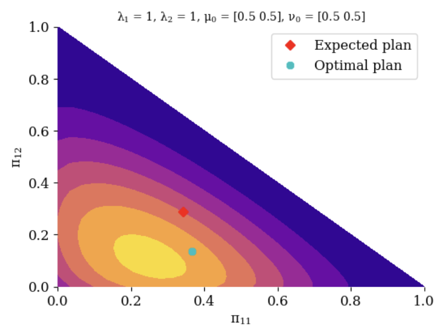
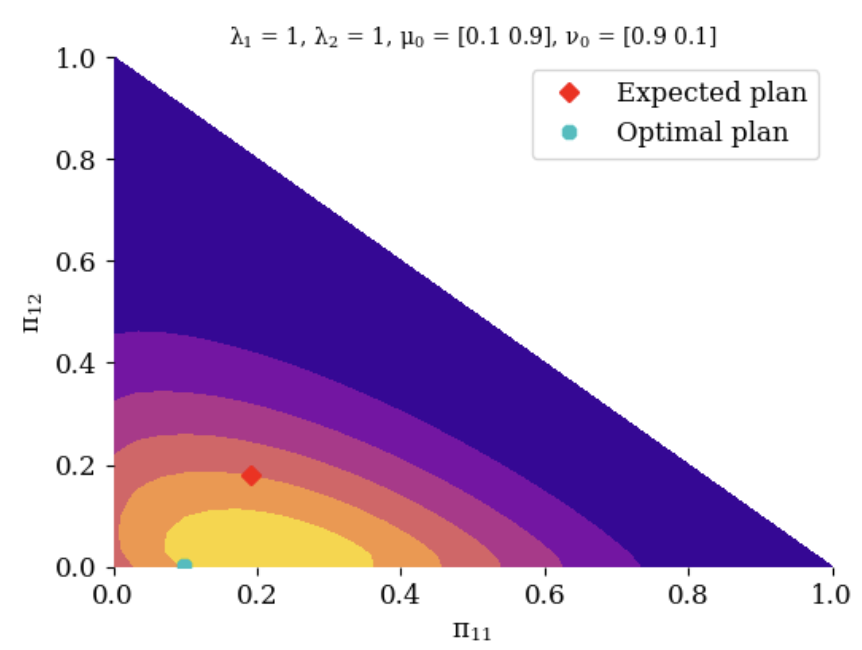
Figure 6: Marginal hyperprior $\mathsf{S}(\pi_{11},\pi_{12}|K)$ for fixed Kantorovitch potentials and various values of the nominal marginals $(\mu_{0},\nu_{0})$. The red and blue dots correspond, respectively, to the projection of the expected transport plan and EOT plan, onto their first two components.

Finally, we explore the influence of the ideal design, and more precisely, the smoothness parameter $\epsilon$ on the location of $\mathsf{S}(\pi_{11},\pi_{12}|K)$. By varying $\epsilon\in\{0.1,0.5,10\}$, it is clear from Figure 7 that this parameter influences the location of the marginal hyperprior, which gradually moves from bottom to left. Meanwhile, we observe — for this specific choice of $\boldsymbol{\lambda}$— that the expected and optimal plans become increasingly close as $\epsilon$ increases. The smoothness $\epsilon$ is another location parameter that can be used to control the shift of the hyperprior.

Figure 7: Contour plots of the marginal hyperprior $\mathsf{S}(\pi_{11},\pi_{12}|K)$, for various values of the smoothness parameter $\epsilon$. The red and blue dots, correspond respectively, to the projection over their first two components, of the expected plan and the optimal plan.

In the next Section, we focus on the derivation of the optimal Kantorovitch potentials $\boldsymbol{\lambda}^{o}$. This requires processing the knowledge constraints $(\eta,\zeta)$ in the hyperprior, by solving the dual program (22). To this aim, we leverage a combination of second-order optimization and MCMC techniques.

Figure 8: A simple schematic of a transport plan in $\Delta_{3}$ simplex with the corresponding nominal marginals. Note that: $\pi_{22}=1-\pi_{11}-\pi_{12}-\pi_{21}$

4.2 Stochastic approximation of the optimal Kantorovitch potentials

In what follows, we propose a methodology to estimate the optimal Kantorovitch potentials $\boldsymbol{\lambda}^{o}$, given the knowledge constraints $K$. Computing these potentials, by means of the dual program in (22), is a critical step in the design of the optimal hyperprior $\mathsf{S}^{o}(\pi|K)$. However, deriving their exact values in high dimensional settings is not trivial, as it requires manipulating the intractable normalising constant (23). The methodology proposed herein approximates these potentials using a combination of Quasi-Newton [Nocedal and Wright, 2006], [Nesterov, 2018] and Hamiltonian Monte Carlo (HMC) [Betancourt, 2017], thus circumventing the need to evaluate $\mathsf{N}(\boldsymbol{\lambda})$. In particular, HMC provides a rigorous and efficient framework for sampling in high dimensional settings: compared to other MCMC techniques, the number of gradient estimation in HMC is less sensitive to the problem’s dimension, making it a convenient choice when generating transport plans [Mangoubi and Smith, 2019].

As established in (22), the optimal Kantorovitch potentials are given by:

$$\boldsymbol{\lambda}^{o}=\operatorname*{argmin}_{\boldsymbol{\lambda}\succeq 0}\left\{\boldsymbol{\lambda}^{\intercal}\boldsymbol{\theta}-\log\left(\mathsf{N}(\boldsymbol{\lambda})\right)\right\}$$ (41)

Let $\varrho(\boldsymbol{\lambda})\equiv\boldsymbol{\lambda}^{\intercal}\boldsymbol{\theta}-\log\left(\mathsf{N}(\boldsymbol{\lambda})\right)$ denote the optimization objective in (41). Its gradient vector can be written conveniently using the following expectation:

$$\begin{split}\nabla_{\boldsymbol{\lambda}}\varrho(\boldsymbol{\lambda})&=\boldsymbol{\theta}-\mathsf{E}_{\mathsf{S}}\bigl{[}\mathsf{R}(\pi)\bigr{]}\end{split}$$ (42)

We define $s_{t}$ and $n_{t}$, the potentials and gradient differentials respectively, as follows: $s_{t}\equiv\boldsymbol{\lambda}^{(t+1)}-\boldsymbol{\lambda}^{(t)}$ and $n_{t}\equiv\nabla\varrho(\boldsymbol{\lambda}^{(t+1)})-\nabla\varrho(\boldsymbol{\lambda}^{(t)})$, where $t>0$ denotes the iteration number in Quasi-Newton. This allows us to write the recursive approximation of the inverse Hessian as follows [Nocedal and Wright, 2006]:

$$\mathsf{H}^{(t+1)}=(\boldsymbol{\mathsf{I}}-\varsigma_{t}s_{t}n_{t}^{\intercal})\mathsf{H}^{(t)}(\boldsymbol{\mathsf{I}}-\varsigma_{t}n_{t}s_{t}^{\intercal})+\varsigma_{t}s_{t}s_{t}^{\intercal}\;\;\;,\;\ \varsigma_{t}\equiv\frac{1}{n_{t}^{\intercal}s_{t}}$$ (43)

where $\boldsymbol{\mathsf{I}}$ denotes the identity matrix. We note that the inverse Hessian $\mathsf{H}^{(t)}$ depends only on the stochastic gradients $\nabla\varrho(\boldsymbol{\lambda}^{(t)})$ (42). Thus, we avoid stability issues when dealing with ill-conditioned stochastic inverse Hessian approximations, as it may happen with high variance MC samplers. Once computed, the gradient and the inverse Hessian are plugged into the usual BFGS iterative updates [Nocedal and Wright, 2006]:

$$\boldsymbol{\lambda}^{(t+1)}\xleftarrow{}\boldsymbol{\lambda}^{(t)}-\rho^{(t)}\mathsf{H}^{(t)}\nabla_{\boldsymbol{\lambda}}\varrho(\boldsymbol{\lambda}^{(t)})$$ (44)

where $\rho^{(t)}>0$ is the step size at the $t^{th}$ iteration in the search direction given by:

$$\mathsf{d}(\boldsymbol{\lambda}^{(t)})\equiv-\mathsf{H}^{(t)}\nabla_{\boldsymbol{\lambda}}\varrho(\boldsymbol{\lambda}^{(t)})$$ (45)

The step size $\rho^{(t)}$ should be adapted carefully to ensure convergence to the global minimum $\boldsymbol{\lambda}^{o}$. It is usually computed by solving an auxiliary line search problem, using techniques such as backtrack line search (BTLS) [Nesterov, 2018]. However, most of line search techniques require the evaluation of the objective $\varrho(\boldsymbol{\lambda})$ at each step, a requirement that can be hardly achieved in our case, for this would entail the approximation of the high dimensional integral $\mathsf{N}(\boldsymbol{\lambda})$ at each iteration. To avoid explicit function evaluations, we propose a simple local approximation, which allows for the estimation of the position of the minimum along the search line (45), based solely on two gradient evaluations [Snyman, 2005].

More precisely, the optimal step size that yields sufficient decrease in the search direction (45) can be found by solving the following problem:

$$\rho^{(t)}_{*}=\operatorname*{argmin}_{\rho\in[0,1]}\varrho(\boldsymbol{\lambda}^{(t)}+\rho\;\mathsf{d}(\boldsymbol{\lambda}^{(t)}))$$ (46)

Assuming that $\varrho$ is locally quadratic at $\boldsymbol{\lambda}^{(t)}$, it follows that solving (46) reduces to finding $\rho$ that satisfies:

$$\varrho(\boldsymbol{\lambda}^{(t)}+\rho\;\mathsf{d}(\boldsymbol{\lambda}^{(t)}))=\varrho(\boldsymbol{\lambda}^{(t)})$$ (47)

Which yields the following optimal step size:

$$\begin{split}\rho^{(t)}_{*}&=\frac{-\mathsf{d}(\boldsymbol{\lambda}^{(t)})^{\intercal}\nabla\varrho(\boldsymbol{\lambda}^{(t)})}{{\mathsf{d}(\boldsymbol{\lambda}^{(t)})}^{\intercal}\nabla^{2}\varrho(\boldsymbol{\lambda}^{(t)})\mathsf{d}(\boldsymbol{\lambda}^{(t)})}\end{split}$$ (48)

Finally, by a second-order Taylor expansion at $\boldsymbol{\lambda}^{(t)}$ and $\boldsymbol{\lambda}^{(t)}+\mathsf{d}(\boldsymbol{\lambda}^{(t)})$, the denominator in (48) can be computed using two gradients estimations, as follows:

$${\mathsf{d}(\boldsymbol{\lambda}^{(t)})}^{\intercal}\nabla^{2}\varrho(\boldsymbol{\lambda}^{(t)})\mathsf{d}(\boldsymbol{\lambda}^{(t)})\approx{\mathsf{d}(\boldsymbol{\lambda}^{(t)})}^{\intercal}\left[\nabla\varrho(\boldsymbol{\lambda}^{(t)}+\mathsf{d}(\boldsymbol{\lambda}^{(t)}))-\nabla\varrho(\boldsymbol{\lambda}^{(t)})\right]$$ (49)

What remains is to compute the gradient terms, which can be estimated using HMC. If $n_{samp}>0$ is the number of independent realizations $\pi^{(t)}$ sampled from the hyperprior at the $t^{th}$ iteration, the expectation in (42) can be approximated as follows:

$$\mathsf{E}_{\mathsf{S}}\bigl{[}\mathsf{R}(\pi)\bigr{]}\approx\frac{1}{n_{samp}}\sum\limits_{i=1}^{n_{samp}}\mathsf{R}(\pi^{(i)})$$ (50)

At each iteration $t$, the error (stopping criterion) is measured by means of the following Newton’s decrement, which corresponds to the inverse Hessian norm of the gradient. This quantity provides a good indication of the proximity to the optimal Kantorovitch potentials:

$$\mathsf{err}\equiv\nabla_{\boldsymbol{\lambda}}\varrho(\boldsymbol{\lambda}^{(t)})^{\intercal}\nabla_{\boldsymbol{\lambda}}^{2}\varrho(\boldsymbol{\lambda}^{(t)})^{-1}\nabla_{\boldsymbol{\lambda}}\varrho(\boldsymbol{\lambda}^{(t)})$$ (51)

Once the optimal potentials $\boldsymbol{\lambda}^{o}$ have been processed, they can be plugged into (21) and the newly formed optimal hyperprior can be used to generate random transport plans, by means of another HMC sampler.

Input: nominal marginals $(\mu_{0},\nu_{0})$, KLD radii $(\eta,\zeta)$, target precision $\tau$, base ideal design $\pi_{\mathsf{I}}$, hierarchical ideal design $\mathsf{S}_{\mathsf{I}}$, number of samples $n_{\mathsf{samp}}$

Result: $\boldsymbol{\lambda}^{o}$

1 Initialization: $t=1$, $\boldsymbol{\lambda}^{(t)}\succeq 0$, $\rho^{(t)}=1$, $\mathsf{H}^{(t)}=\boldsymbol{\mathsf{I}}$, $\mathsf{err}=\infty$ ;

2 while $\tau<\mathsf{err}$ do

3       Sample $\{\pi^{(t)}_{l}\}_{l=1}^{n_{\mathsf{samp}}}\sim\mathsf{S}(\pi|K_{-\boldsymbol{\lambda}},\boldsymbol{\lambda}^{(t)})$ $\triangleright$ HMC sampler. $K_{-\boldsymbol{\lambda}}$ denotes all parameters in the set $K$, except $\boldsymbol{\lambda}$ ;

4       Estimate $\mathsf{E}_{\mathsf{S}(\pi|K_{-\boldsymbol{\lambda}},\boldsymbol{\lambda}^{(t)})}\left[\mathsf{R}(\pi)\right]$ ;

5       Estimate $\nabla_{\boldsymbol{\lambda}}\varrho(\boldsymbol{\lambda}^{(t)})$ ;

6       Compute $\tilde{\boldsymbol{\lambda}}^{(t+1)}\leftarrow\tilde{\boldsymbol{\lambda}}^{(t)}-\mathsf{H}^{(t)}\nabla\varrho(\boldsymbol{\lambda}^{(t)})$ ;

7       Sample $\{\tilde{\pi}^{(t+1)}_{l}\}_{l=1}^{n_{\mathsf{samp}}}\sim\mathsf{S}(\pi|K_{-\boldsymbol{\lambda}},\tilde{\boldsymbol{\lambda}}^{(t+1)})$ ;

8       Estimate $\nabla_{\boldsymbol{\lambda}}\varrho(\tilde{\boldsymbol{\lambda}}^{(t+1)})$ ;

9       Compute $\rho_{*}^{(t)}$ ;

10       Update $\boldsymbol{\lambda}^{(t+1)}\xleftarrow{}\boldsymbol{\lambda}^{(t)}-\rho_{*}^{(t)}\mathsf{H}^{(t)}\nabla\varrho(\boldsymbol{\lambda}^{(t)})$ ;

11       Compute $s_{t}$, $n_{t}$ and $\varsigma_{t}$ ;

12       Update $\mathsf{H}^{(t+1)}\leftarrow(\boldsymbol{\mathsf{I}}-\varsigma_{t}s_{t}n_{t}^{\intercal})\mathsf{H}^{(t)}(\boldsymbol{\mathsf{I}}-\varsigma_{t}n_{t}s_{t}^{\intercal})+\varsigma_{t}s_{t}s_{t}^{\intercal}$ ;

13       Update $\mathsf{err}$ ;

14       Update $t\leftarrow t+1$

return $\boldsymbol{\lambda}^{(t+1)}$

Algorithm 1 Approximation of the Kantorovitch potentials

Remark 4.

Computational complexity. In the proposed Algorithm (1), we replace each approximation of the normalising constant $\mathsf{N}(\boldsymbol{\lambda})$ (23) with two gradient approximations. Therefore, the overall computational complexity is mainly driven by the sampling operations in line $3$ and $7$ of the Algorithm, whose complexity is, in turn, contingent upon the number of gradient evaluation used in the leapfrog integrator of the HMC sampler [Betancourt, 2017]. Under certain regularity conditions, this number is of order $\mathcal{O}(\sqrt{mn})$ [Mangoubi and Smith, 2019]. Though these conditions are not totally satisfied in our case (see Remark 5), this already serves as a good indicator so as to assess the complexity of our proposed method. Using, for example, a Mean-Field Variational Bayes method — which assumes that all the parameters $\pi_{i,j}$ are independent — to approximate the normalising constant $\mathsf{N}(\boldsymbol{\lambda})$ at each iteration of the Quasi-Newton method, yields a time complexity that is linear in the number of parameters, i.e. of order $\mathcal{O}(mn)$.

Remark 5.

On HMC mixing properties. It is worth noting that the main convergence results of HMC, when sampling from a log-concave function $\mathsf{e}^{-f}$, require strongly convex and Lipshitz smooth (i.e. Lipshitz $\nabla f$) potential functions $f$ [Chen and Vempala, 2019]. However, the KLD being not Lipshitz smooth, this results in our case in a longer integration time and higher variance in the obtained samples. There exist other sampling techniques, that relax the regularity assumptions on $f$, which may improve the quality of samples and reduce the mixing time. For the time being, we will use HMC while carefully tuning its main parameters (integrator step size, adaptation step, etc.) and leave the derivation of specialized samplers for a separate work.

5 HFPD-OT for algorithmic fairness

The goal of algorithmic fairness in machine learning is to correct algorithmic biases that may arise in data acquisition and model training workflows, resulting in unjustified disparities in the predicted outcomes. It is also a compelling setting for HFPD-OT, since the latter can benefit from randomized and dynamic transport plans to elicit fair transport strategies in the presence of uncertainty. Randomized transport plans can also play a key role in providing the modeller’s with the tools and mechanisms to quantify and reason about the uncertainty in data repair problems, instead of relying on a single and uninformative point estimate.

To appreciate the implications of randomization and diversity allowed by HFPD-OT in this context, we propose to explore the following two questions: (i) the design and elicitation of long-term fair transport policies in the face of uncertainty and (ii) randomized OT plans for robust and generalizable data repair algorithms . The interplay between randomization and fairness is an exciting but largely under-explored area in machine learning and our goal in this Section is by no means to exhaustively address all the related challenges. This introductory work is rather an attempt to explore these questions from the lens of HFPD-OT and formalize in mathematical language the associated key concepts. For this purpose, let’s consider the following experimental setting:

• $m=n=d=20$

• $\epsilon=10^{-3}$

• $\mathsf{C}(x,y)=\|x-y\|^{2}$

• $\eta=2$, $\zeta=2$

• $\lambda_{\mathsf{I},1}=0.5$, $\lambda_{\mathsf{I},2}=0.5$

• Generation of the empirical marginals : $\mu_{t}\sim\mathcal{Dir}(\mathcal{u}_{0})$, $\nu_{t}\sim\mathcal{Dir}(\mathcal{u}_{1})$, where: $\mathcal{u}_{0}\sim\mathcal{U}_{[0,m]}$ and $\mathcal{u}_{1}\sim\mathcal{U}_{[0,n]}$. $\mathcal{U}_{[a,b]}$ denotes the Uniform distribution on the interval $[a,b]$, $\mathcal{Dir}(\mathcal{u})$ is the Dirichlet distribution with base measure $\mathcal{u}$ and $t\in\mathbb{N}$ is a discrete index. We further impose the moment constraints in (17), (18) via a simple rejection-acceptance scheme.

• HMC sampler:

  • step size: $s=0.3$

  • leapfrog step size: $l=6$

  • burn-in steps: $8000$

  • adaptation steps: $0.8\times\text{burn-in steps}$

  • target acceptance probability: $0.6$

5.1 Long-term fairness via diversity and randomization

The classical OT setting is concerned with the optimization of the expected transport cost (6). This optimization problem, however, is unfair by design, unfairness being a direct consequence of certainty equivalence, which assumes perfect knowledge of the input marginals. As we have argued throughout this paper, the nominal marginals are noisy, random realizations of some underlying stochastic process. Failing to model this uncertainty implies that the classical OT solution $\pi^{o}$ can deviate substantially from the true unknown optimal transport policy $\pi_{\mathsf{true}}$:

$$\mathcal{P}(|\pi^{o}-\pi_{\mathsf{true}}|>\varepsilon)\xrightarrow[]{\eta\to\infty,\;\zeta\to\infty}1$$ (52)

where $\varepsilon>0$ is a lower bound quantifying the regret incurred by such a sub-optimal transport policy. Thus, a myopic assignment of OT plans implies that some participants may be wrongly and permanently served or unserved, based on a biased representation of the world (Figure 10(a)).

In contrast to this deterministic allocation of resources, HFPD-OT allows us to design randomized transportation strategies. Randomized policies arise quite often in machine learning, where the decision of a single model is replaced by a random combination of diverse models, and have shown powerful results, both heuristically and theoretically [Brown et al., 2005], [Grgić-Hlača et al., 2017]. Our goal is to apply the same principle to elicit fairer outcomes. Importantly, we would like to achieve long-term fairness by relying solely on the diversity of transport plans, without requiring the overhaul of the original optimization problem, nor the integration of an explicit fairness constraint in (6). We do so by replacing the single, fixed OT plan with a sequence of random transport policies. By doing so, each contract will experience a sequence of diverse transport decisions which should yield, in the limit, an overall fairer resource allocation strategy.

First, let’s gain some intuition about the role of randomization and diversity in the design of fair transport policies. Let $y_{0}\in\mathbb{\Omega}_{Y}$ be a target node and $\pi(.|Y=y_{0})$ the corresponding random conditional distribution, as illustrated in Figure 1(c). $y_{0}$ can be a consumer of a resource or an asset in a portfolio allocation problem and $\pi(x|Y=y_{0})$ is the mass/resource allocated by the source node $x\in\mathbb{\Omega}_{X}$. In the base OT setting, this conditional distribution is deterministic and invariable. On the other hand, the HFPD-OT formalism relaxes this assumption and views this conditional distribution as a stochastic process. We define $c_{y_{0}}$, the random total transport cost associated with $y_{0}$, as follows:

$$c_{y_{0}}\equiv\sum_{x\in\mathbb{\Omega}_{X}}\pi(x|Y=y_{0})\mathsf{C}(x,y_{0})\;\;,\;\;\pi\sim\mathsf{S}^{o}$$ (53)

As a simple, yet important, consequence of the random nature of $c_{y_{0}}$, we can derive a lower bound on the probability that the latter decreases below the minimum average transport cost between $\mu_{0}$ and $\nu_{0}$ — or equivalently the 2-Wasserstein distance — using Markov’s inequality, which reads (Figure 1(c)):

$$1-\frac{\mathsf{E}_{\mathsf{S}^{o}(\pi_{x|y_{0}})}(c_{y_{0}})}{W_{2}^{2}(\mu_{0},\nu_{0})}<\mathcal{P}(c_{y_{0}}\leq W_{2}^{2}(\mu_{0},\nu_{0}))$$ (54)

where $W_{2}^{2}(\mu_{0},\nu_{0})$ is defined as follows:

$$W_{2}^{2}(\mu_{0},\nu_{0})\equiv\min_{\pi\in\mathbb{\Pi}(\mu_{0},\nu_{0})}\mathsf{E}_{(X,Y)\sim\pi}(\mathsf{C}(x,y))$$ (55)

Though the lower bound in (54) may be unsophisticated, it suffices to convey the main point here: by the very nature of the random process $c_{y_{0}}$, each node in the target domain has a non-zero probability of experiencing a transport cost lower than the average cost.

The setting we have contemplated so far is mainly static. To reason further about the connection between fairness and randomized policies, we direct momentarily our attention to a dynamic setting, where a sequence of independent transport plans $\pi^{(k)}$, indexed by $k\in\mathbb{N}$, is sampled using the optimal hyperprior $\mathsf{S}^{o}(\pi|K)$ (Figure 9). $\pi^{(k)}_{i,j}$ denotes the $(i,j)^{th}$ contract of the $k^{th}$ random transport plan. In this dynamic context, an interesting quantity that measures the diversity in the transport problem, which is essentially unavailable in the base OT setting, is the sequence of eligible contracts $\{\mathbb{E}_{K}^{(k)}\}_{k\in\mathbb{N}}$ where:

$$\mathbb{E}_{K}^{(k)}\equiv\bigl{\{}(i,j)\in\mathsf{supp}(\pi^{(k)}),\;\text{s.t.}\;\pi_{i,j}^{(k)}\;\text{is active}\bigr{\}}$$ (56)

$\mathsf{supp}(\cdot)$ denotes the support of the enclosed distribution. The set of eligible contracts corresponds to the contracts that are active or — using an economic terminology — those that are recruited over time, given the knowledge constraints $K$. The notion of activity can be instantiated as required by the experimental setting. For example, in an engineering problem, it may correspond to contracts associated with a mass higher than a threshold fixed by some design specifications. In a neural translation problem, it may be the attention weights higher than an activation threshold. This quantity clearly depends on $(\eta,\zeta)$: the set of eligible contracts diminishes as uncertainty in the marginals decreases and the hyperprior degenerates to the statistical manifold with support in $\mathbb{\Pi}(\mu_{0},\nu_{0})$ (28).

Our formal definition of fairness, as allowed by HFPD-OT, relies on the principle of equal treatment of eligible contracts in the face of uncertainty: when uncertainty about the marginals is substantial, a fair transport policy requires that the rate of beneficial outcome is the same for all eligible contracts. More precisely, via a dynamic assignment of transport policies, we would like to guarantee, asymptotically and for each of the contracts in $\bigcup_{k\in\mathbb{N}}\mathbb{E}_{K}^{(k)}$, an equal chance of beneficial outcome. On the other hand, it is critical to recover the classical FPD-OT policy as more knowledge about the marginals is accumulated. In mathematical terms, the long-term fairness allowed by HFPD-OT interpolates between the two following regimes:

• Under incomplete specification of the marginals ($\eta\rightarrow\infty$, $\zeta\rightarrow\infty$), equal treatment of contracts reads as (Figure 1(b)):

  $$\mathsf{E}_{\mathsf{S}^{o}(\pi_{ij})}\bigl{[}\mathbb{1}\bigl{(}\pi_{i,j}>\bar{m})\bigr{]}=\frac{1}{2}\;\;,\;\forall(i,j)\in\bigcup_{k>0}\mathbb{E}_{K}^{(k)}$$ (57)

  where $\bar{m}$ is the average mass transported from $\mathbb{\Omega}_{X}$ to $\mathbb{\Omega}_{Y}$: $\bar{m}\equiv\frac{1}{d^{2}}$.

• As the specification of the marginals improves with the accumulation of knowledge ($\eta\rightarrow 0$, $\zeta\rightarrow 0$), we naturally converge towards the FPD-OT solution (32), characterized by:

  $$\mathsf{E}_{\mathsf{S}^{o}(\pi_{ij})}\bigl{[}\mathbb{1}\bigl{(}\pi_{i,j}=\pi^{o}_{i,j})\bigr{]}=1\;\;,\;\forall(i,j)\in\bigcup_{k>0}\mathbb{E}_{K}^{(k)}$$ (58)

For the purpose of illustration, let’s fix the Kantorovitch potentials to arbitrarily small values: $\lambda_{1}=\lambda_{2}=0.05$ (or equivalently large $(\eta,\zeta)$) and generate a sequence of frequency maps, whose entries correspond to the probability of each contract being associated with a mass higher than the average mass $\bar{m}$. Figures 10(b), 10(c) and 10(d) show the frequency maps as a function of the number of samples, after observing respectively $N=10$, $50$ and $100$ pairs of empirical marginals. In the limit, the frequency maps stabilize and eventually converge to the fair regime defined in (57).

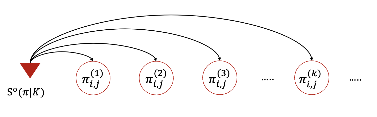
Figure 9: A sequence of independent contracts $\{\pi_{i,j}^{(k)}\}_{k\geq 1}$ is sampled from the optimal hyperprior, allowing for the contract $\pi_{i,j}$ to experience a sequence of diverse transport policies, as equivalently depicted in Figure 4(b). Fairness is achieved in the long-term and corresponds, in the regime of high uncertainty, to a uniform distribution of positive outcomes, where each contract has the same probability of experiencing a higher than average associated mass.

(a) EOT plan computed between nominal marginals $\mu_{0}$ and $\nu_{0}$.

(b) Frequency map after $N=10$ random transport plans.

(c) Frequency map after $N=50$ random transport plans.

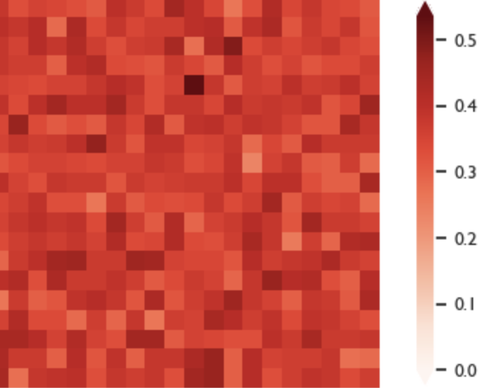
(d) Frequency map after $N=100$ random transport plans.

Figure 10: The optimal transport plan in the base OT case is unfair by design since contracts associated with a higher cost are systematically excluded (Figure (a)). In contrast with the base OT, randomization gives naturally rise to a fairer regime in the limit, as more transport plans are observed. Each entry in the frequency maps shows the probability of the corresponding contract being associated with a transported mass above the average mass $\bar{m}$. As expected, the frequency maps stabilize over time and converge to a uniform configuration (Figures (b), (c), (d)). In all these experiments, we choose: $\lambda_{1}=\lambda_{2}=0.05$

Finally, we propose a new metric that quantifies diversity in HFPD-OT. To this aim, we can lean on the rich literature on diversity quantification in information and ecological systems [Jost, 2006]. We choose diversity (or equivalently, the exponential entropy) instead of the classical entropy, since the former is a more intuitive way of quantifying diversity in a system. More precisely, we use the $1-$diversity index, also known in machine learning as perplexity, which we define in the context of HFPD-OT as follows: [Diversity index] Let $\mathsf{S}^{o}(\pi|K)$ be the optimal HFPD-OT hyperprior and let $m\times n$ be the dimension of the corresponding random transport plan. The 1-diversity index (or equivalently, perplexity) associated with $\mathsf{S}^{o}$ is:

$$D(\mathsf{S}^{o}(\pi|K))\equiv\mathsf{E}_{\mathsf{S}^{o}}\left[\exp\bigl{(}\mathsf{H}(\pi)\bigr{)}\right]$$ (59)

where $\mathsf{H}(\pi)$ denotes the entropy of $\pi$:

$$\mathsf{H}(\pi)\equiv-\sum_{i=1}^{m}\sum_{j=1}^{n}\pi_{i,j}\log(\pi_{i,j})$$ (60)

$m\times n$ is called the richness index. It is equal to the total number of contracts in the transport plan. The more knowledge about the empirical marginals we accumulate over time, the less uncertainty and therefore diversity in the optimal hyperprior (1). To empirically demonstrate this inverse relationship, we compute the diversity index $D$ (59) for different values of the Kantorovitch potentials. The results, averaged over 100 MC runs, are shown in Figure 11. The plot clearly shows the decreasing trend, where larger values of the Kantorovitch potentials — or equivalently, smaller uncertainty radii $(\eta,\zeta)$ – yield smaller diversity indices.

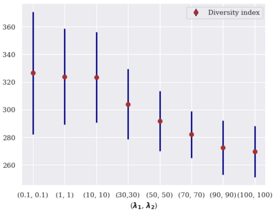
Figure 11: Diversity indices obtained for different values of the Kantorovitch potentials ${\boldsymbol{\lambda}}$ and averaged over 100 MC runs. Higher values of the potentials induce a lower uncertainty in the marginals and therefore less diversity.

Remark 6.

The HFPD-OT diversity indices obtained in Figure 11 should be contrasted with the index in the base EOT setting, which is by construction null. One should also observe that the variance of the samples, though decreasing with larger Kantorovitch potentials, remains relatively high. We believe that a sampling strategy specifically tailored for the problem at hand, that utilises the geometry of the space of transport plans, will result in a lower variance.

5.2 Learning robust data repair with HFPD-OT

To demonstrate further our HFPD-OT method, we examine the problem of data repair for bias mitigation in machine learning models. Considering a simple 1-dimensional data repair problem, we instantiate the nominal marginals as the distributions of an observed feature $Z\in\mathbbm{R}$, conditioned on some binary protected attribute $A\in\{0,1\}$ (gender, age, ethnicity, etc.): $\mu_{0}=P(Z|A=0)$, $\nu_{0}=P(Z|A=1)$, and we study the question of fairness elicitation using randomized transport policies in HFPD-OT.

Most of data repair techniques rely on decoupling the decision variable $g(Z)$ from the protected attribute $A$ [Barocas et al., 2018]:

$$g(Z)\perp\!\!\!\perp A$$ (61)

where $\perp\!\!\!\perp$ denotes statistical independence and $g$ is the learned statistical model. One way to achieve this independence is to drive the conditional distributions towards a common target distribution, the challenge being to reach a satisfactory level of fairness while minimally damaging the data. In particular, Wasserstein-based repair techniques use the Fréchet mean in the Wasserstein space (or the Wasserstein barycentre) as a target distribution [McCann, 1997], [Agueh and Carlier, 2011]. In the following, we consider the fixed support Wasserstein barycentre repair method proposed in [Feldman et al., 2015], [Johndrow and Lum, 2017], [Gordaliza et al., 2019], which is described by this system of equations:

$$\left\{\begin{aligned} x^{(r)}_{t,i}=w_{0}x_{t,i}+dw_{1}\sum_{j=1}^{d}\pi^{*}_{i,j}y_{t,j},\;\;\forall i\in[d]\\ y^{(r)}_{t,j}=w_{1}y_{t,j}+dw_{0}\sum_{i=1}^{d}\pi^{*}_{i,j}x_{t,i}\;\;\forall j\in[d]\end{aligned}\right.$$ (62)

$w_{0}$ and $w_{1}$ are the Wasserstein barycentre weights, fixed here to: $w_{0}=w_{1}=0.5$ and $(\mu_{t},\nu_{t})$ denotes the $t^{th}$ pair of marginals in a sequence of independently observed empirical marginals (• ‣ 5). Note that this repair scheme is not total in that it yields two, a.s. disjoint clusters. We denote the clusters obtained by repairing the $t^{th}$ pair of marginals by $\mathcal{X}_{t}\equiv\{x^{(r)}_{t,1},x^{(r)}_{t,2},\dots x^{(r)}_{t,m}\}$ and $\mathcal{Y}_{t}\equiv\{y^{(r)}_{t,1},y^{(r)}_{t,2},\dots y^{(r)}_{t,n}\}$, respectively.

In the original algorithm of [Feldman et al., 2015], $\pi^{*}$ is instantiated as the deterministic EOT transport plan between the empirical marginals $\mu_{t}$ and $\nu_{t}$ (8). We propose to investigate new repair techniques in the context of HFPD-OT by replacing $\pi^{*}$ with randomized transport plans, sampled from the optimal hyperprior (21). More precisely, we study the two following questions: 1. how to leverage randomized transport plans to process distributional fairness metrics, hence generating robust estimates of the quality of the data repair process and 2. how to design robust data repair strategies that generalize to new observed empirical marginals using stochastic transport policies in lieu of the OT plan.

5.3 Distributional fairness proxies

We first investigate the idea of distributional fairness proxies enabled by randomized HFPD-OT transport plans. To this aim, we consider the following repair strategies:

1. Deterministic EOT repair: for each pair of empirical marginals $(\mu_{t},\nu_{t})_{t\in\mathbbm{N}}$, the corresponding optimal transport plan $\pi^{o}_{t}$ (8) is designed and used in the repair process described in (62), in place of $\pi^{*}$. This reference scheme can be used as a yardstick by which to judge various repair alternatives, mainly the randomized HFPD-OT repair scheme.

2. Randomized HFPD-OT repair: in this case, each of the empirical marginals is repaired using a random realization sampled from the optimal hyperprior (21): $\pi\sim\mathsf{S}^{o}$, which is used in lieu of $\pi^{*}$ in (62).

The pseudo-code is provided in Algorithm (2). To assess the quality of data repair, we rely on the simple inter-cluster Euclidean distance between $\mathcal{X}_{t}$ and $\mathcal{Y}_{t}$, denoted by $\mathsf{ICD}_{t}$ and defined as follows:

$$\mathsf{ICD}_{t}\equiv\sum_{i=1}^{d}|x^{(r)}_{t,i}-y^{(r)}_{t,i}|^{2}$$ (63)

Input: Nominal marginals $(\mu_{0}$, $\nu_{0})$, Wasserstein weights $(w_{1}$, $w_{2})$, empirical marginals $(\mu_{t}$, $\nu_{t})$, base ideal design $\pi_{\mathsf{I}}$, hierarchical ideal design $\mathsf{S}_{\mathsf{I}}$, number of samples $S$.

1 Initialization: $\mathsf{ICD}\leftarrow\mathsf{NULL}$

Result: Distribution over $\mathsf{ICD}$

2 Process the optimal hyperprior: $\mathsf{S}^{o}(\pi|K)$ $\triangleright$ See Algorithm 1

3 for s = 1 …S do

4       Generate $\pi_{s}\sim\mathsf{S}^{o}(\pi|K)$

5       Compute $x_{t,i,s}^{(r)}=w_{1}x_{t}+dw_{2}\pi_{s}^{\intercal}y_{t}\;\;\forall\;i\in[d]$ ;

6       Compute $y_{t,j,s}^{(r)}=w_{2}y_{t}+dw_{1}\pi_{s}^{\intercal}x_{t}\;\;\forall\;j\in[d]$ ;

7       Compute $\mathsf{ICD_{s}}$ ;

8       Update $\mathsf{ICD}\leftarrow\mathsf{ICD}\cup\mathsf{ICD_{s}}$

Algorithm 2 Algorithm for processing distributional fairness proxies

Figure 12(a) shows the distribution of $\mathsf{ICD}_{t}$ obtained for a particular pair a marginals $\{\mu_{t},\nu_{t}\}$, plotted against the deterministic EOT point estimate. In the deterministic EOT repair scheme, the empirical marginals are assumed to be observed perfectly, yielding a single transport plan and eventually a single point estimate of the fairness proxy. Opposed to this certainty-equivalence mindset, we can use the HFPD-OT optimal hyperprior to sample multiple independent transport plans and use these instances to repair the empirical marginals. The first step consists in learning the optimal Kantorovitch potentials using Algorithm 1; this yields the optimal hyperprior $\mathsf{S}^{o}(\pi|K)$. Under the stationarity assumption, we can sample independent instances of transport plans $\pi\sim\mathsf{S}(\pi|K)$ and use each instance to compute a measure of fairness. The resulting distribution of $\mathsf{ICD}$ conveys far more insights about the data repair quality than a unique and possibly biased point estimate. This allows the modeller to reason about the uncertainty in the repair problem and implement mitigation mechanisms before using the repaired data in downstream learning tasks.

5.4 Robust data repair

We will now address the second question, related to robust data repair. The main goal is to study how randomized transport plans can help generalize the existing data repair mechanism to new empirical marginals, beyond the nominal marginals. As usual, we start by learning the optimal hyperprior $\mathsf{S}^{o}$, by processing the optimal Kantorovitch potentials for fixed nominal marginals $(\mu_{0},\nu_{0})$. We then observe a sequence of independent and stationary marginals $\{\mu_{t},\nu_{t}\}_{t\in\mathbb{N}}$. Each pair is repaired using the scheme described in (62), where $\pi^{*}$ is instantiated respectively as:

1. $\pi^{o}$ (8) for the deterministic EOT repair.

2. $\pi\sim\mathsf{S}^{o}$(21) for the randomized HFPD-OT scheme.

3. And finally as $\overset{\circ}{\pi}\equiv\pi^{o}(\mu_{0},\nu_{0})$, corresponding to the EOT plan designed between the nominal marginals $\mu_{0}$ and $\nu_{0}$, for what is called nominal OT. The purpose of this last repair scheme is to study the generalization of the transport plan processed between the nominal marginals, to new empirical marginals without any specific tuning.

As before, the $\mathsf{ICD}$ is used as a proxy for assessing fairness quality. Two perfectly aligned clusters will yield 0 ICD — or equivalently, maximum fairness — in that the protected attribute $A$ is no longer predictable from the decision rule $g(Z)$. However, such an extreme repair scheme is not desirable because the distortion induced in the data is so important that the predictive performance of the model $g$ is impeded. For this reason, we keep track of a second metric, that measures the induced distortion during the repair process. The original and repaired distributions having a.s. disjoint supports, the Wasserstein distance remains the most suitable distance to keep track of such a distortion:

$$W_{2}^{2}(\mu_{t},\mu^{(r)}_{t})\equiv\min_{\pi\in\mathbb{\Pi}(\mu_{t},\mu^{(r)}_{t})}\mathsf{E}_{(X,Y)\sim\pi}(\mathsf{C}(x,y))$$ (64)

where $\mu^{(r)}_{t}$ denotes the repaired version of $\mu_{t}$. The results are shown in Figure 12, with the following notable observations:

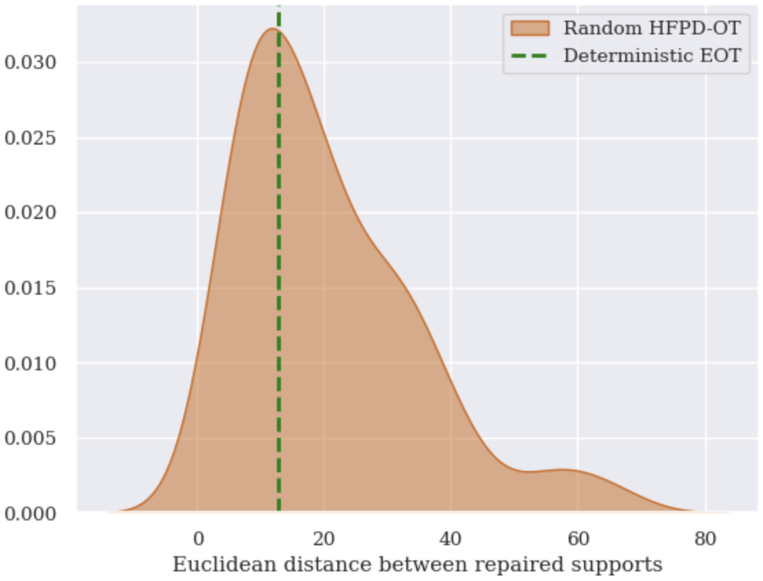
(a) Distributional fairness measure

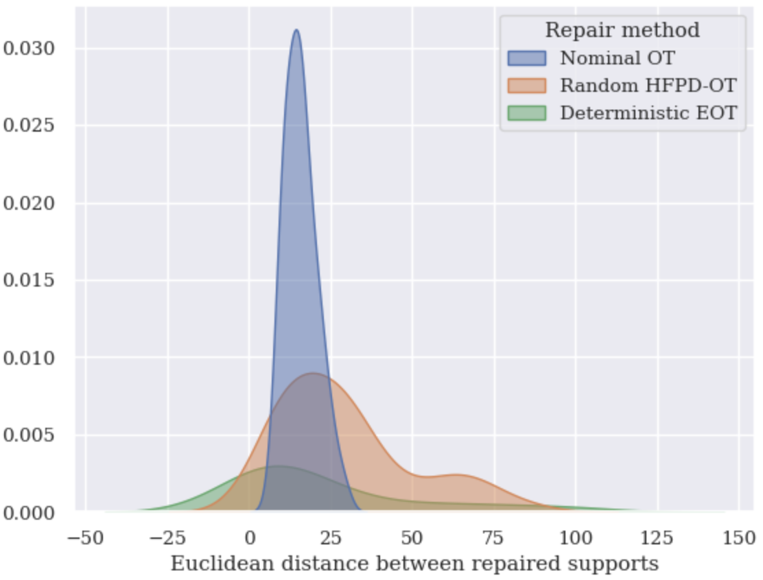
(b) Data repair quality

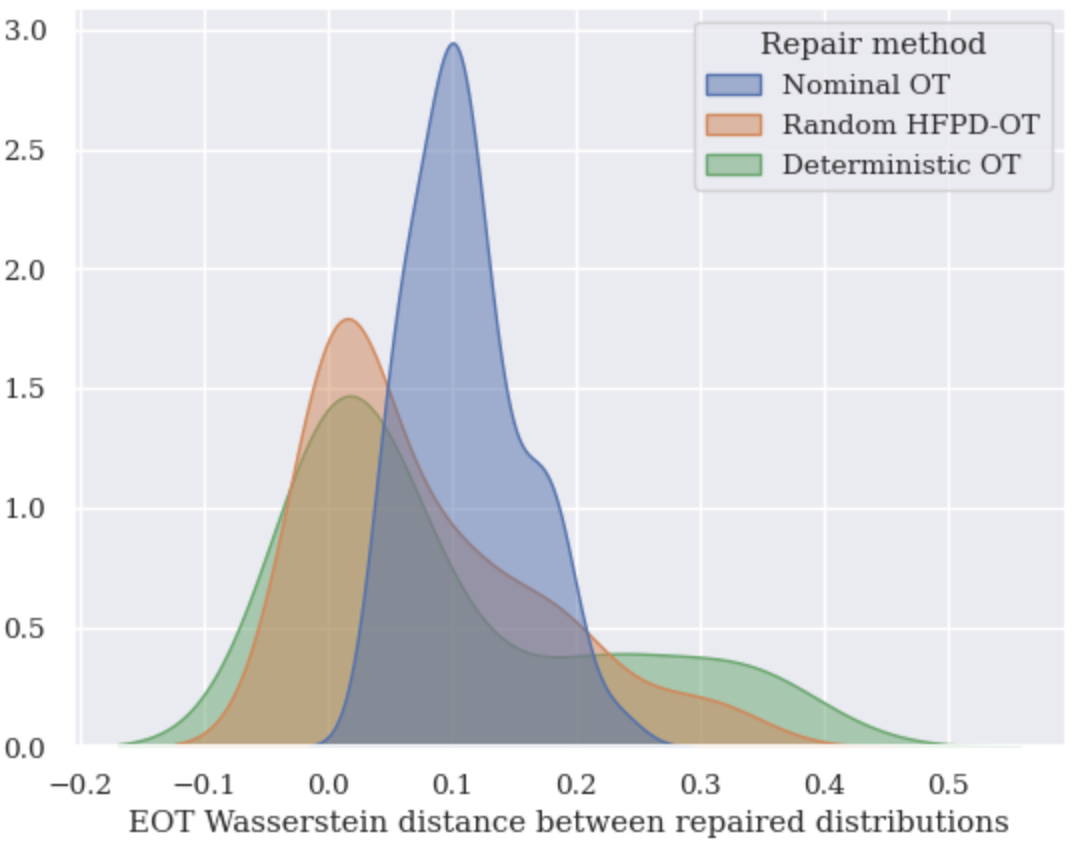
(c) Data repair distortion

Figure 12: Experiments for robust data repair. Randomized transport policies are explored in the context of data repair for fairness elicitation. (a): each random transport plan produces an estimate of the fairness proxy, yielding a distribution over fairness measures instead of a single point estimate. (b) Gaussian KDE of the distribution of ICD computed for $S=50$ independent empirical marginals. Each marginal is repaired using: (1) the deterministic EOT plan between the two empirical marginals, (2) a random sample from the HFPD-OT hyperprior and (3) the EOT plan designed using the nominal marginals. (c): Gaussian KDE of the data repair distortion computed for the previously stated repair schemes.

• First, we note the relative symmetry between the repair quality in Figure 12(b) and the induced distortion in Figure 12(c), which highlights the natural tension that exists between these two measurements: higher repair quality (i.e. lower ICD) induces higher distortion (i.e. higher Wasserstein distance).

• Looking at the repair quality in Figure 12(b), we find that the repair scheme based on $\overset{\circ}{\pi}$ induces a sharp, low-variance distribution of ICD. Since this strategy relies solely on the OT plan learned from the nominal marginals, it does not adapt the repair scheme to specific empirical marginals, hence the low variance. However this comes at the expense of higher distortion, as depicted in Figure 12(c).

• We also note in Figure 12(b) that deterministic EOT repair scheme based on $\pi^{o}$ has the highest variance among all schemes, due probably to its sensitivity to outliers, where highly skewed distributions may lead to larger ICD. Comparatively, a repair strategy using a random HFPD-OT sample is more robust, showing a relatively smaller variance.

• Looking at the corresponding distortion in Figure 12(c), it is interesting to observe that both deterministic EOT and random HFPD-OT schemes yield a largely comparable distortion. Hence, randomized transport plans yield a more robust repair strategy in that samples from the hyperprior act as summary statistics that are less sensitive to pathological marginals. Importantly, this robustness does not degrade the distortion, which is comparable with what is observed in the deterministic EOT repair case.

6 Conclusions and next steps

This paper recasts the optimal transport problem into a broader class of fully probabilistic design and generalized Bayesian inference techniques. In this new formalism, the transport plan is no longer regarded as a crisp, deterministic object, but is modelled as a random (i.e. uncertain) distribution in a hierarchical Bayesian setting. This is in clear contrast with the existing, certainty-equivalence-based OT paradigm. In this way, we augment the classical (base-level) OT framework with the necessary tools to reason about uncertainty and design robust transport algorithms. In this new hierarchical setting, the object of interest is no longer the optimal transport plan, which may not even exist — since the marginals are themselves noisy, uncertain realizations of some underlying stochastic process — but is rather the optimal hyperprior, which is effectively a generative model over the set of transport plans.

We now recall some key results on HFPD-OT, obtained in this paper:

• The functional form of the optimal hyperprior has been characterized in both the non-parametric and parametric settings. Importantly, we proved that the HFPD-OT setting is a generalization of the classical EOT in that the optimal transport plan can be recovered asymptotically when uncertainty in the marginals decreases.

• Considering the parametric setting, we proposed an algorithm to approximate the Kantorovitch potentials and described some of the inferential properties of the hyperprior, highlighting its shape and location parameters.

• To illustrate the concept of HFPD-OT, we studied the problem of algorithmic fairness from two perspectives. First, we explored the role of randomization and diversification in eliciting fairer transport policies in the long-term — compared to a static and myopic OT plan — and proposed a new metric for fairness quantification, based on the notion of diversity. Second, we studied the question of robust data repair using Wasserstein barycentres. We started by proposing an improved version of the data repair algorithm in [Feldman et al., 2015], by exchanging the OT plan for a random transport plan. This same randomization principle is used to produce a distribution of fairness proxies, allowing for a comprehensive analysis of uncertainty in the data repair problem.

There are important open questions and improvements that will be studied in subsequent work. The suite of algorithms leveraged here enables a first approximation of the hyperprior, but there is substantial room for improvement of these algorithms, both in terms of the quality of the transport plans sampled from the hyperprior and the overall computational complexity. Interestingly, sampling from the hyperprior may require new Markov chain Monte Carlo (MCMC) techniques, ones which leverage further the geometry of the support of $\mathsf{S}^{o}(\pi|K)$, thus expanding the existing computational methods with a new set of specialized techniques. Having access to the optimal hyperprior opens up many possible use cases, where robust and generalizable transport strategies are critical. The set of applications we covered in this paper are orientated mainly towards fairness elicitation and robust data repair. However, there exist other applications in machine learning and economics that we will address in subsequent work. Finally, a notable contribution of this paper has been to expand duality results from classical setting in OT to the hierarchical framework of HFPD-OT. However, key theoretical results in classical OT, mainly those related to its geometry ([Gangbo and McCann, 1996], [Villani, 2008], etc.), need careful consideration in the context of the relaxed transport design framework of HFPD-OT.

7 Appendix: proof of strong duality in Theorem 3.1 (step 3)

The following additional mathematical definitions are required, supplementing the preliminaries in Section 2.2.

• Besides being compact, we assume henceforth that $\mathbb{\Omega}_{X}$ and $\mathbb{\Omega}_{Y}$ are Hausdorff sets. This separability property guarantees uniqueness of limits and sequences.

• From compactness of $\mathbb{\Omega}_{X}$ and $\mathbb{\Omega}_{Y}$, it follows, by the Riesz-Markov-Kakutani Theorem [Folland, 1999], that the topological dual of $\mathbb{C}(\mathbb{\Omega}_{X}\times\mathbb{\Omega}_{Y})$ — the set of continuous functions on $\mathbb{\Omega}_{X}\times\mathbb{\Omega}_{Y}$ — is a the set of Radon measures with support in $\mathbb{\Omega}_{X}\times\mathbb{\Omega}_{Y}$. This also implies that $\mathbb{C}(\mathbb{\Omega}_{X}\times\mathbb{\Omega}_{Y})$ is a Banach space. Thus, by the Banach-Alaoglu Theorem, $\mathbbm{P}(\mathbb{\Omega}_{X}\times\mathbb{\Omega}_{Y})$ is compact in the weak-* topology [Billingsley, 1999].

• The previous compactness result allows us to again invoke the Riesz-Markov-Kakutani representation Theorem, which states that the topological dual of $\mathbb{C}(\mathbbm{P}(\mathbb{\Omega}_{X}\times\mathbb{\Omega}_{Y}))$ is the space of Radon measures with support in $\mathbbm{P}(\mathbb{\Omega}_{X}\times\mathbb{\Omega}_{Y})$. We denote this dual space by $\mathbb{S}$. The canonical duality pairing reads as follows [Folland, 1999]:

  $$<f,\mathsf{S}>\equiv\int_{\mathbbm{P}(\mathbb{\Omega}_{X}\times\mathbb{\Omega}_{Y})}fd\mathsf{S}$$ (65)

  with $f\in\mathbb{C}(\mathbbm{P}(\mathbb{\Omega}_{X}\times\mathbb{\Omega}_{Y}))$ and $\mathsf{S}\in\mathbb{S}$. Later in the proof, we will constrain $\mathbb{S}$ to the set of hierarchical (probability) distributions.

• If $\mathsf{O}:\mathbb{S}\rightarrow\mathbbm{R}^{p}$ is a linear map, its adjoint is defined as: $\mathsf{O}^{*}\colon\mathbbm{R}^{p}\rightarrow\mathbb{C}(\mathbb{P}(\mathbb{\Omega}_{X}\times\mathbb{\Omega}_{Y}))$ such that:

  $$<\mathsf{O}(\mathsf{S}),z>=<\mathsf{S},\mathsf{O}^{*}(z)>$$ (66)

  for $\mathsf{S}\in\mathbb{S}$ and $z\in\mathbb{R}^{p}$.

• $f^{*}$ denotes the Legendre-Fenchel transform of $f$ defined in $\mathbb{C}(\mathbbm{P}(\mathbb{\Omega}_{X}\times\mathbb{\Omega}_{Y}))$. It is given by:

  $$f^{*}(u)\equiv\sup_{v\in\mathbb{C}(\mathbbm{P}(\mathbb{\Omega}_{X}\times\mathbb{\Omega}_{Y}))}(<u,v>-f(v))$$ (67)

• $\mathsf{dom}(h)$ denotes the effective domain of the function $h\in\mathbb{C}(\mathbb{P}(\mathbb{\Omega}_{X}\times\mathbb{\Omega}_{Y}))$, defined as: $\mathsf{dom}(h)\equiv\{\pi\in\mathbb{P}(\mathbb{\Omega}_{X}\times\mathbb{\Omega}_{Y})\;|\;h(\pi)<\infty\}$.

• Our proof relies on the notion of decomposable spaces, as originally defined in [Rockafellar, 1971]. A space is decomposable if it is stable under bounded alterations over sets of finite measure.

• Let $\mathbb{L}(\mathbb{P}(\mathbb{\Omega}_{X}\times\mathbb{\Omega}_{Y}))$ denote the set of integrable functions, defined in $\mathbb{P}(\mathbb{\Omega}_{X}\times\mathbb{\Omega}_{Y})$. $\mathbb{L}(\mathbb{P}(\mathbb{\Omega}_{X}\times\mathbb{\Omega}_{Y}))$ is clearly decomposable, since it satisfies the following conditions [Rockafellar, 1971]:

  • $\mathbb{L}(\mathbb{P}(\mathbb{\Omega}_{X}\times\mathbb{\Omega}_{Y}))$ contains every bounded and measurable functions defined on $\mathbb{P}(\mathbb{\Omega}_{X}\times\mathbb{\Omega}_{Y})$.

  • If $h\in\mathbb{L}(\mathbb{P}(\mathbb{\Omega}_{X}\times\mathbb{\Omega}_{Y}))$ and $\mathbb{l}\in\mathcal{F}_{\mathbb{\Omega}_{\mathsf{H}}}$ is an arbitrary set of finite measure in $\mathbb{P}(\mathbb{\Omega}_{X}\times\mathbb{\Omega}_{Y})$ (3), then $\mathbb{L}(\mathbb{P}(\mathbb{\Omega}_{X}\times\mathbb{\Omega}_{Y}))$ contains $\chi_{\mathbb{l}}\cdot h$, where $\chi_{\mathbb{l}}$ is the indicator function of the set $\mathbb{l}$, given by: $\chi_{\mathbb{l}}(\pi)=1\;\text{if}\;\pi\in\mathbb{l}\;\text{and}\;0\;\text{o.w.}$

For the sake of completeness, we recall the main duality Theorem [Rockafellar, 1974] in the general setting, before specialising it to our problem later in the proof: [Fenchel-Rockafellar] Let $(E,E^{*})$ and $(F,F^{*})$ be two topologically paired spaces. Let $\mathsf{O}\colon E\rightarrow F$ be a continuous linear operator and $\mathsf{O}^{*}\colon F^{*}\rightarrow E^{*}$ its adjoint. Let f and g be lower semicontinuous and proper convex functions defined on E and F, respectively. If the following qualification condition is satisfied: $\exists\;y^{*}\in dom(g^{*})$   s.t.   $f^{*}$ is continuous at $\mathsf{O}^{*}(y^{*})$, then:

$$\max_{x\in E}-f(-x)-g(\mathsf{O}(x))=\min_{y^{*}\in F^{*}}f^{*}(\mathsf{O}^{*}(y^{*}))+g^{*}(y^{*})$$ (68)

Proof.

Let’s consider the Primal problem in (14). Using Fubini’s Theorem and the Bayesian hierarchical modelling consistency condition stated in (10), it is easy to show that this original problem can be formulated equivalently, over the set of hyperpriors $\mathbb{S}$, as follows:

$$(P):\;\;\;\;\;\mathsf{S}^{o}\in\operatorname*{argmin}_{\mathsf{S}\in\mathbb{S}}\left\{\mathsf{D}_{\mathsf{KL}}\bigl{(}\mathsf{S}(\pi|K)||\tilde{\mathsf{S}}(\pi|K)\bigr{)}\right\}$$ (69)

subject to:

$$\left\{\begin{aligned} \mathsf{E}_{\mathsf{S}}(\mathsf{D}_{\mathsf{KL}}(\mu||\mu_{0}))\leq\eta\\ \mathsf{E}_{\mathsf{S}}(\mathsf{D}_{\mathsf{KL}}(\nu||\nu_{0}))\leq\zeta\end{aligned}\right.$$

where $\tilde{\mathsf{{S}}}$ is defined in (20). The constraints involve the following linear map:

$$\mathsf{I}(\mathsf{S})\equiv\int_{\mathbbm{P}(\mathbb{\Omega}_{X}\times\mathbb{\Omega}_{Y})}\mathsf{S}(\pi|K)d\mathcal{L}(\pi)$$ (70)

besides our usual moment constraints:

$$\mathsf{O}_{1}(\mathsf{S})\equiv\mathsf{E}_{\mathsf{S}}(\mathsf{D}_{\mathsf{KL}}(\mu||\mu_{0}))\;\;\;,\;\;\mathsf{O}_{2}(\mathsf{S})\equiv\mathsf{E}_{\mathsf{S}}(\mathsf{D}_{\mathsf{KL}}(\nu||\nu_{0}))$$ (71)

For convenience, we denote by $\bar{\mathsf{O}}$ the linear map given by:

$$\bar{\mathsf{O}}(\mathsf{S})\equiv(\mathsf{I}(\mathsf{S}),\mathsf{O}_{1}(\mathsf{S}),\mathsf{O}_{2}(\mathsf{S}))\in\mathbbm{R}^{3}$$ (72)

As usual, we can use the indicator function to encode the constraints directly in the objective $(P)$ , yielding the following equivalent unconstrained problem:

$$(P^{\prime}):\;\;\;\mathsf{S}^{o}\in\operatorname*{argmin}_{\mathsf{S}}\left\{\mathsf{D}_{\mathsf{KL}}\bigl{(}\mathsf{S}(\pi|K)||\tilde{\mathsf{S}}(\pi|K)\bigr{)}+g_{0}(\bar{\mathsf{O}}(\mathsf{S}))\right\}$$ (73)

where we define $g_{0}$ as follows:

$$g_{0}(z_{0},z_{1},z_{2})\equiv\iota_{[0,\eta]}(z_{0})+\iota_{[0,\zeta]}(z_{1})+\iota_{\{1\}}(z_{2})\;\;,\;\;(z_{0},z_{1},z_{2})\in\mathbbm{R}^{3}$$ (74)

Let’s start by deriving the Legendre-Fenchel dual of $\bar{\mathsf{O}}(\cdot)$, $g_{0}(\cdot)$ and $\mathsf{D}_{\mathsf{KL}}(\cdot||\cdot)$, respectively. By the definition of the adjoint in (72), it is straightforward to show that $\mathsf{\bar{O}}^{*}$ is given by:

$$\mathsf{\bar{O}}^{*}(\lambda_{1},\lambda_{2},\lambda_{3})=\lambda_{1}\mathsf{D}_{\mathsf{KL}}(\mu||\mu_{0})+\lambda_{2}\mathsf{D}_{\mathsf{KL}}(\nu||\nu_{0})+\lambda_{3}\;\;,\;\;(\lambda_{1},\lambda_{2},\lambda_{3})\in\mathbbm{R}^{3}$$ (75)

Moreover, applying the definition of Legendre-Fenchel transform (67) yields the following conjugate of $g_{0}$:

$$\begin{split}g_{0}^{*}(\lambda_{1},\lambda_{2},\lambda_{3})=\lambda_{1}\eta+\lambda_{2}\zeta+\lambda_{3}\end{split}$$ (76)

We now turn our attention to the conjugate of $\mathsf{D}_{\mathsf{KL}}(\cdot||\cdot)$. To this aim, we first consider the following integral functional [Rockafellar, 1971]:

$$\mathcal{I}_{\mathsf{f}}(u)\colon\mathbb{C}(\mathbbm{P}(\mathbb{\Omega}_{X}\times\mathbb{\Omega}_{Y})) \longrightarrow\mathbbm{R}$$ (77)

$$u \longmapsto\int_{\mathbbm{P}(\mathbb{\Omega}_{X}\times\mathbb{\Omega}_{Y})}\mathsf{f}(\pi,u(\pi))d\mathcal{L}(\pi)$$ (78)

where:

$$\mathsf{f}(\pi,u(\pi))\equiv\tilde{\mathsf{S}}(\pi|K)\exp\bigl{(}u(\pi)-1\bigr{)}$$ (79)

$\mathsf{f}(\pi,\cdot)$ is clearly an integrable, proper and convex function. As we saw earlier, the space $\mathbb{L}(\mathbbm{P}(\mathbb{\Omega}_{X}\times\mathbb{\Omega}_{Y}))$ is decomposable. Therefore, by Theorem 2 in [Rockafellar, 1971], we can perform the Legendre-Fenchel transform of $\mathcal{I}_{\mathsf{f}}$ through the integral sign and write:

$$\mathcal{I}^{*}_{\mathsf{f}}(u)=\mathcal{I}_{\mathsf{f}^{*}}(\mathsf{S})\equiv\int_{\mathbbm{P}(\mathbb{\Omega}_{X}\times\mathbb{\Omega}_{Y})}\mathsf{f}^{*}(\pi,u(\pi))d\mathcal{L}(\pi)$$ (80)

$\mathsf{f}^{*}$ is obtained using again the definition of the Fenchel-Rockafellar transform (67):

$$\begin{split}\mathsf{f}^{*}(\pi,\mathsf{S}(\pi|K))&\equiv\sup_{u\in\mathbb{C}(\mathbbm{P}(\mathbb{\Omega}_{X}\times\mathbb{\Omega}_{Y}))}\bigl{\{}u(\pi)\mathsf{S}(\pi|K)-\mathsf{f}(\pi,u(\pi))\bigr{\}}\\ &=\mathsf{S}(\pi|K)\log\Bigl{(}\frac{\mathsf{S}(\pi|K)}{\tilde{\mathsf{S}}(\pi|K)}\Bigr{)}\end{split}$$ (81)

It follows that:

$$\mathcal{I}^{*}_{\mathsf{f}}(x)=\mathsf{D}_{\mathsf{KL}}(\mathsf{S}||\tilde{\mathsf{S}})$$ (82)

There exists at least one hyperprior $\mathsf{S}\in\mathbb{S}$ s.t. $\mathsf{f}^{*}$ is an integrable function of $\pi$ (consider for instance $\mathsf{S}=\mathsf{\tilde{S}}$). It follows, by Theorem 1 in [Rockafellar, 1971], that $\mathcal{I}_{\mathsf{f}}$ is a well-defined convex functional. Thus, the conjugacy operator acts as an involution on $\mathcal{I}_{\mathsf{f}}$, yielding:

$$\mathsf{D}_{\mathsf{KL}}^{*}=\mathcal{I}_{\mathsf{f}}^{**}=\mathcal{I}_{\mathsf{f}}$$ (83)

Going back to our main Theorem in (7), it is obvious that $\mathsf{D}_{\mathsf{KL}}(\cdot||\cdot)$ and $g_{0}(\cdot)$ are lower semicontinuous, proper and convex. Furthermore, $\mathsf{D}_{\mathsf{KL}}^{*}(\cdot||\cdot)$ is continuous everywhere w.r.t the uniform norm (Theorem 4 in [Rockafellar, 1974]). It follows that strong duality holds and that the primal and dual problems are equal, the dual reading as follows:

$$\begin{split}(D):\;\;\;\;\sup_{(\lambda_{1},\lambda_{2},\lambda_{3})\in\mathbbm{R}^{3}}\left\{-\int_{\mathbbm{P}(\mathbb{\Omega}_{X}\times\mathbb{\Omega}_{Y})}\tilde{\mathsf{S}}(\pi|K)\exp\bigl{(}\bar{\mathsf{O}}^{*}(-\lambda_{1},-\lambda_{2},-\lambda_{3})-1\bigr{)}d\mathcal{L}(\pi)-\lambda_{1}\eta-\lambda_{2}\zeta-\lambda_{3}\right\}\end{split}$$ (84)

One can simplify further the latter result by maximizing (84) w.r.t $\lambda_{3}$ for fixed $(\lambda_{1},\lambda_{2})$, yielding the following value for $\lambda^{o}_{3}$:

$$\lambda^{o}_{3}=\log\left(\int_{\mathbbm{P}(\mathbb{\Omega}_{X}\times\mathbb{\Omega}_{Y})}\tilde{\mathsf{S}}(\pi|K)\exp\left(-\lambda_{1}\mathsf{D}_{\mathsf{KL}}(\mu||\mu_{0})-\lambda_{2}\mathsf{D}_{\mathsf{KL}}(\nu||\nu_{0})-1\right)d\mathcal{L}(\pi)\right)$$ (85)

By substituting $\lambda^{o}_{3}$ back into (84), we obtain (22).

The optimality condition:

$$0\in\partial\mathsf{D}_{\mathsf{KL}}(\mathsf{S}(\pi|K))+\partial{g_{0}}\bigl{(}\bar{O}(\mathsf{S}\bigr{)})$$ (86)

implies that the primal and dual optimal solutions should satisfy the following extremality conditions [Rockafellar, 1967]:

$$\left\{\begin{aligned} \mathsf{S}^{o}\in\partial{\mathcal{I}_{\mathsf{f}}(-\mathsf{O}^{*}(\lambda_{1},\lambda_{2}))}\;\;\;\mathcal{L}-a.e.\\ (-\lambda_{1}^{o},-\lambda_{2}^{o})\in\partial{g_{0}\bigl{(}\mathsf{O}_{1}(\mathsf{S}),\mathsf{O}_{2}(\mathsf{S})\bigr{)}}\end{aligned}\right.$$

$\mathcal{I}_{\mathsf{f}}$ being differentiable everywhere, its sub-differential reduces to the usual gradient, leading to the same optimal hyperprior derived earlier using information processing arguments (21):

$$\mathsf{S}^{o}\propto\exp\left(-\lambda_{1}^{o}\mathsf{D}_{\mathsf{KL}}(\mu||\mu_{0})\right)\tilde{\mathsf{S}}(\pi|K)\exp\left(-\lambda_{2}^{o}\mathsf{D}_{\mathsf{KL}}(\nu||\nu_{0})\right)\;\;\;\mathcal{L}-a.e.$$ (87)

On the other hand, noting that the sub-differential of the indicator function $g_{0}$ is the normal cone $\bar{\mathsf{N}}_{\mathbb{Q}}\bigl{(}\mathsf{O}_{1}(\mathsf{S}),\mathsf{O}_{2}(\mathsf{S})\bigr{)}$, defined as follows:

$$\bar{\mathsf{N}}_{\mathbb{Q}}\bigl{(}\mathsf{O}_{1}(\mathsf{S}),\mathsf{O}_{2}(\mathsf{S})\bigr{)}\equiv\left\{v\in\mathbbm{R}^{2}\;\;|\;\;v^{\intercal}\left[\boldsymbol{x}-\begin{bmatrix}\mathsf{O}_{1}(\mathsf{S})\\ \mathsf{O}_{2}(\mathsf{S})\end{bmatrix}\right]\preceq 0,\forall\boldsymbol{x}\in[0,\eta]\times[0,\zeta]\right\}$$ (88)

the following optimality conditions are obtained, for the special choice of $\boldsymbol{x}=(\eta,\zeta)$ plugged in (88):

$$\left\{\begin{aligned} \lambda_{1}^{o}\Bigl{(}\eta-\mathsf{E}_{\mathsf{S}}\bigl{(}\mathsf{D}_{\mathsf{KL}}(\mu||\mu_{0}\bigr{)}\Bigr{)}\geq 0\\ \lambda_{2}^{o}\Bigl{(}\zeta-\mathsf{E}_{\mathsf{S}}\bigl{(}\mathsf{D}_{\mathsf{KL}}(\nu||\nu_{0}\bigr{)}\Bigr{)}\geq 0\end{aligned}\right.$$

Thus: $\boldsymbol{\lambda}\equiv(\lambda_{1}^{o},\lambda_{2}^{o})\succeq 0$. ∎

References

- Agueh and Carlier [2011] M. Agueh and G. Carlier. Barycenters in the Wasserstein space. SIAM Journal on Mathematical Analysis, 43(2):904–924, 2011. doi: 10.1137/100805741. URL https://doi.org/10.1137/100805741.
- Arjovsky et al. [2017] M. Arjovsky, S. Chintala, and L. Bottou. Wasserstein generative adversarial networks. In D. Precup and Y. W. Teh, editors, Proceedings of the 34th International Conference on Machine Learning, volume 70 of Proceedings of Machine Learning Research, pages 214–223. PMLR, 06–11 Aug 2017. URL https://proceedings.mlr.press/v70/arjovsky17a.html.
- Barocas et al. [2018] S. Barocas, M. Hardt, and A. Narayanan. Fairness and machine learning limitations and opportunities. 2018. URL https://api.semanticscholar.org/CorpusID:113402716.
- Ben-Tal et al. [2009] A. Ben-Tal, L. Ghaoui, and A. Nemirovski. Robust Optimization. 08 2009. ISBN 9781400831050. doi: 10.1515/9781400831050.
- Bernardo [1979] J. M. Bernardo. Expected Information as Expected Utility. The Annals of Statistics, 7(3):686 – 690, 1979. doi: 10.1214/aos/1176344689. URL https://doi.org/10.1214/aos/1176344689.
- Betancourt [2017] M. Betancourt. A conceptual introduction to Hamiltonian Monte Carlo. arXiv: Methodology, 2017. URL https://api.semanticscholar.org/CorpusID:88514713.
- Billingsley [1999] P. Billingsley. Convergence of probability measures. Wiley Series in Probability and Statistics: Probability and Statistics. John Wiley & Sons Inc., New York, second edition, 1999. ISBN 0-471-19745-9. A Wiley-Interscience Publication.
- Bissiri et al. [2016] P. G. Bissiri, C. C. Holmes, and S. G. Walker. A general framework for updating belief distributions. Journal of the Royal Statistical Society Series B: Statistical Methodology, 78(5):1103–1130, feb 2016. doi: 10.1111/rssb.12158. URL https://doi.org/10.1111%2Frssb.12158.
- Borwanker et al. [1971] J. Borwanker, G. Kallianpur, and B. L. S. P. Rao. The Bernstein-von Mises theorem for Markov processes. The Annals of Mathematical Statistics, 42(4):1241–1253, 1971. ISSN 00034851. URL http://www.jstor.org/stable/2240025.
- Brown et al. [2005] G. Brown, J. Wyatt, R. Harris, and X. Yao. Diversity creation methods: A survey and categorisation. Information Fusion, 6:5–20, 03 2005. doi: 10.1016/j.inffus.2004.04.004.
- Carlier et al. [2017] G. Carlier, V. Duval, G. Peyré, and B. Schmitzer. Convergence of entropic schemes for optimal transport and gradient flows. SIAM Journal on Mathematical Analysis, 49(2):1385–1418, 2017. doi: 10.1137/15M1050264. URL https://doi.org/10.1137/15M1050264.
- Chen and Vempala [2019] Z. Chen and S. S. Vempala. Optimal convergence rate of Hamiltonian Monte Carlo for strongly logconcave distributions, 2019. URL https://arxiv.org/abs/1905.02313.
- Chizat et al. [2016] L. Chizat, G. Peyré, B. Schmitzer, and F.-X. Vialard. Scaling algorithms for unbalanced transport problems. arXiv: Optimization and Control, 2016. URL https://api.semanticscholar.org/CorpusID:119312616.
- Courty et al. [2017] N. Courty, R. Flamary, D. Tuia, and A. Rakotomamonjy. Optimal transport for domain adaptation. IEEE Transactions on Pattern Analysis and Machine Intelligence, 39(9):1853–1865, 2017. doi: 10.1109/TPAMI.2016.2615921.
- Cuturi [2013] M. Cuturi. Sinkhorn distances: Lightspeed computation of optimal transport. In C. Burges, L. Bottou, M. Welling, Z. Ghahramani, and K. Weinberger, editors, Advances in Neural Information Processing Systems, volume 26. Curran Associates, Inc., 2013. URL https://proceedings.neurips.cc/paper_files/paper/2013/file/af21d0c97db2e27e13572cbf59eb343d-Paper.pdf.
- Delahaye et al. [2019] D. Delahaye, S. Chaimatanan, and M. Mongeau. Simulated Annealing: From Basics to Applications, pages 1–35. Springer International Publishing, Cham, 2019. ISBN 978-3-319-91086-4. doi: 10.1007/978-3-319-91086-4_1. URL https://doi.org/10.1007/978-3-319-91086-4_1.
- El Moselhy and Marzouk [2012] T. A. El Moselhy and Y. M. Marzouk. Bayesian inference with optimal maps. Journal of Computational Physics, 231(23):7815–7850, 2012. ISSN 0021-9991. doi: https://doi.org/10.1016/j.jcp.2012.07.022. URL https://www.sciencedirect.com/science/article/pii/S0021999112003956.
- Feldman et al. [2015] M. Feldman, S. A. Friedler, J. Moeller, C. Scheidegger, and S. Venkatasubramanian. Certifying and removing disparate impact. In Proceedings of the 21th ACM SIGKDD International Conference on Knowledge Discovery and Data Mining, KDD ’15, page 259–268, New York, NY, USA, 2015. Association for Computing Machinery. ISBN 9781450336642. doi: 10.1145/2783258.2783311. URL https://doi.org/10.1145/2783258.2783311.
- Folland [1999] G. B. Folland. Real Analysis : Modern Techniques and Their Applications. Wiley, New York, 1999.
- Frogner and Poggio [2019] C. Frogner and T. Poggio. Fast and flexible inference of joint distributions from their marginals. In K. Chaudhuri and R. Salakhutdinov, editors, Proceedings of the 36th International Conference on Machine Learning, volume 97 of Proceedings of Machine Learning Research, pages 2002–2011. PMLR, 09–15 Jun 2019. URL https://proceedings.mlr.press/v97/frogner19a.html.
- Galichon [2016] A. Galichon. Optimal Transport Methods in Economics. Princeton University Press, 2016. URL http://www.jstor.org/stable/j.ctt1q1xs9h.
- Gangbo and McCann [1996] W. Gangbo and R. J. McCann. The geometry of optimal transportation. Acta Mathematica, 177(2):113 – 161, 1996. doi: 10.1007/BF02392620. URL https://doi.org/10.1007/BF02392620.
- Goodman [1953] L. A. Goodman. Ecological regressions and behavior of individuals. American Sociological Review, 18:663, 1953. URL https://api.semanticscholar.org/CorpusID:147056159.
- Gordaliza et al. [2019] P. Gordaliza, E. D. Barrio, G. Fabrice, and J.-M. Loubes. Obtaining fairness using optimal transport theory. In K. Chaudhuri and R. Salakhutdinov, editors, Proceedings of the 36th International Conference on Machine Learning, volume 97 of Proceedings of Machine Learning Research, pages 2357–2365. PMLR, 09–15 Jun 2019. URL https://proceedings.mlr.press/v97/gordaliza19a.html.
- Grgić-Hlača et al. [2017] N. Grgić-Hlača, M. B. Zafar, K. P. Gummadi, and A. Weller. On fairness, diversity and randomness in algorithmic decision making, 2017.
- Guerreiro et al. [2023] N. M. Guerreiro, P. Colombo, P. Piantanida, and A. F. T. Martins. Optimal transport for unsupervised hallucination detection in neural machine translation, 2023.
- Jeffreys [1939] H. Jeffreys. Theory of Probability. Clarendon Press, Oxford, England, 1939.
- Johndrow and Lum [2017] J. E. Johndrow and K. Lum. An algorithm for removing sensitive information: application to race-independent recidivism prediction, 2017.
- Jost [2006] L. Jost. Entropy and diversity. Oikos, 113(2):363–375, 2006. doi: https://doi.org/10.1111/j.2006.0030-1299.14714.x. URL https://nsojournals.onlinelibrary.wiley.com/doi/abs/10.1111/j.2006.0030-1299.14714.x.
- Kracík and Kárný [2005] J. Kracík and M. Kárný. Merging of data knowledge in Bayesian estimation. In International Conference on Informatics in Control, Automation and Robotics, volume 2, pages 229–232, 2005.
- Kárný and Kroupa [2012] M. Kárný and T. Kroupa. Axiomatisation of fully probabilistic design. Information Sciences, 186(1):105–113, 2012. ISSN 0020-0255. doi: https://doi.org/10.1016/j.ins.2011.09.018. URL https://www.sciencedirect.com/science/article/pii/S0020025511004750.
- Mallasto et al. [2021] A. Mallasto, M. Heinonen, and S. Kaski. Bayesian inference for optimal transport with stochastic cost. In Proceedings of The 13th Asian Conference on Machine Learning, volume 157 of Proceedings of Machine Learning Research, pages 1601–1616. PMLR, 2021.
- Mangoubi and Smith [2019] O. Mangoubi and A. Smith. Mixing of Hamiltonian Monte Carlo on strongly log-concave distributions 2: Numerical integrators. In K. Chaudhuri and M. Sugiyama, editors, Proceedings of the Twenty-Second International Conference on Artificial Intelligence and Statistics, volume 89 of Proceedings of Machine Learning Research, pages 586–595. PMLR, 16–18 Apr 2019. URL https://proceedings.mlr.press/v89/mangoubi19a.html.
- Mathon et al. [2014] B. Mathon, F. Cayre, P. Bas, and B. Macq. Optimal transport for secure spread-spectrum watermarking of still images. Image Processing, IEEE Transactions on, 23:1694–1705, 04 2014. doi: 10.1109/TIP.2014.2305873.
- McCann [1997] R. J. McCann. A convexity principle for interacting gases. Advances in Mathematics, 128:153–179, 1997. URL https://api.semanticscholar.org/CorpusID:123005604.
- Nesterov [2018] Y. Nesterov. Lectures on Convex Optimization. Springer Publishing Company, Incorporated, 2nd edition, 2018. ISBN 3319915770.
- Nocedal and Wright [2006] J. Nocedal and S. J. Wright. Numerical Optimization. Springer, New York, NY, USA, 2e edition, 2006.
- Peyré and Cuturi [2019] G. Peyré and M. Cuturi. Computational optimal transport: With applications to data science. Foundations and Trends® in Machine Learning, 11(5-6):355–607, 2019.
- Quinn [2012] A. Quinn. Recursive inference for inverse problems using variational Bayes methodology. In 1st International ICST Workshop on New Computational Methods for Inverse Problems. ACM, 2012.
- Quinn et al. [2016] A. Quinn, M. Kárný, and T. V. Guy. Fully probabilistic design of hierarchical Bayesian models. Information Sciences, 369:532–547, 2016. ISSN 0020-0255. doi: https://doi.org/10.1016/j.ins.2016.07.035. URL https://www.sciencedirect.com/science/article/pii/S0020025516305163.
- Quinn et al. [2017] A. Quinn, M. Kárný, and T. V. Guy. Optimal design of priors constrained by external predictors. Int. J. Approx. Reasoning, 84(C):150–158, 2017.
- Quinn et al. [2024] A. Quinn, S. Boufelja, M. Corless, and R. Shorten. Fully probabilistic design for optimal transport. Communications in Optimization Theory, 2024. To appear.
- Rockafellar [1967] R. T. Rockafellar. Duality and stability in extremum problems involving convex functions. Pacific Journal of Mathematics, 21(1):167 – 187, 1967.
- Rockafellar [1971] R. T. Rockafellar. Integrals which are convex functionals. II. Pacific Journal of Mathematics, 39(2):439 – 469, 1971.
- Rockafellar [1974] R. T. Rockafellar. Conjugate duality and optimization. 1974. URL https://api.semanticscholar.org/CorpusID:9072945.
- Saumier et al. [2015] L.-P. Saumier, B. Khouider, and M. Agueh. Optimal transport for particle image velocimetry: Real data and postprocessing algorithms. SIAM Journal on Applied Mathematics, 75(6):2495–2514, 2015. ISSN 00361399. URL http://www.jstor.org/stable/43895788.
- Savage [1971] L. J. Savage. Elicitation of personal probabilities and expectations. Journal of the American Statistical Association, 66(336):783–801, 1971. doi: 10.1080/01621459.1971.10482346. URL https://www.tandfonline.com/doi/abs/10.1080/01621459.1971.10482346.
- Shore and Johnson [1980] J. Shore and R. Johnson. Axiomatic derivation of the principle of maximum entropy and the principle of minimum cross-entropy. IEEE Transactions on Information Theory, 26(1):26–37, 1980. doi: 10.1109/TIT.1980.1056144.
- Sklar [1959] M. J. Sklar. Fonctions de repartition à n dimensions et leurs marges. 1959. URL https://api.semanticscholar.org/CorpusID:127105744.
- Snyman [2005] J. Snyman. A gradient-only line search method for the conjugate gradient method applied to constrained optimization problems with severe noise in the objective function. International Journal for Numerical Methods in Engineering, 62:72 – 82, 01 2005. doi: 10.1002/nme.1189.
- Séjourné et al. [2023] T. Séjourné, G. Peyré, and F.-X. Vialard. Chapter 12 - unbalanced optimal transport, from theory to numerics. In E. Trélat and E. Zuazua, editors, Numerical Control: Part B, volume 24 of Handbook of Numerical Analysis, pages 407–471. Elsevier, 2023. doi: https://doi.org/10.1016/bs.hna.2022.11.003. URL https://www.sciencedirect.com/science/article/pii/S1570865922000230.
- Villani [2008] C. Villani. Optimal Transport: Old and New. Springer, 2008.
- Wakefield [2004] J. Wakefield. Ecological inference for 2x2 tables (with discussion). Journal of the Royal Statistical Society Series A, 167:385–445, 08 2004. doi: 10.1111/j.1467-985x.2004.02046.x.