Don’t You (Project Around Discs)? Neural Network Surrogate and Projected Gradient Descent for Calibrating an Intervertebral Disc Finite Element Model

Abstract

Accurate calibration of finite element (FE) models of human intervertebral discs (IVDs) is essential for their reliability and application in diagnosing and planning treatments for spinal conditions. Traditional calibration methods are computationally intensive, requiring iterative, derivative-free optimization algorithms that often take hours or days to converge.

This study addresses these challenges by introducing a novel, efficient, and effective calibration method for an L4-L5 IVD FE model using a neural network (NN) surrogate. The NN surrogate predicts simulation outcomes with high accuracy, outperforming other machine learning models, and significantly reduces the computational cost associated with traditional FE simulations. Next, a Projected Gradient Descent (PGD) approach guided by gradients of the NN surrogate is proposed to efficiently calibrate FE models. Our method explicitly enforces feasibility with a projection step, thus maintaining material bounds throughout the optimization process.

The proposed method is evaluated against state-of-the-art Genetic Algorithm (GA) and inverse model baselines on synthetic and in vitro experimental datasets. Our approach demonstrates superior performance on synthetic data, achieving a Mean Absolute Error (MAE) of 0.06 compared to the baselines’ MAE of 0.18 and 0.54, respectively. On experimental specimens, our method outperforms the baseline in 5 out of 6 cases. Most importantly, our approach reduces calibration time to under three seconds, compared to up to 8 days per sample required by traditional calibration. Such efficiency paves the way for applying more complex FE models, enabling accurate patient-specific simulations and advancing spinal treatment planning.

[label1]organization=Department of Diagnostic and Interventional Neuroradiology, Klinikum rechts der Isar, Technical University of Munich,city=Munich, country=Germany

[label2]organization=Institute for AI in Medicine, School of Computation, Information and Technology, Technical University of Munich,city=Munich, country=Germany

[label3]organization=Department of Trauma and Reconstructive Surgery, University Hospital Halle, Martin-Luther-University Halle-Wittenberg, city=Halle (Saale), country=Germany

[label4]organization=Department of Mechanical Engineering, Federal University of Santa Catarina, city=Florianópolis, country=Brazil

[label5]organization=Department of Mechanical Engineering, Federal University of Santa Maria, city=Av. Santa Maria, country=Brazil

[label6]organization=Associate Professorship of Sport Equipment and Sport Materials, School of Engineering and Design, Technical University of Munich, city=Munich, country=Germany

1 Introduction

Finite element (FE) simulations are a well-established tool in orthopedics and spine research, providing significant value for diagnosing and planning treatments for conditions like scoliosis, fractures, degenerative disc disease, and osteoporosis [1]. Advances in patient-specific models improve surgical planning and enable personalized adjustments to treatment [1]. However, accurate numerical modeling of intervertebral discs (IVDs) encounters substantial challenges, such as structural complexity, patient-specific variability, and the necessity for selecting appropriate material definitions [2, 3].

Calibration or Parameter Estimation of an FE model ensures its accuracy and validity by finding input parameters such that the model output closely matches reported in vitro experimental measurements for particular specimens and geometries. This process is crucial because relying solely on material properties from the literature often fails to capture specific mechanical behaviors, particularly for varying geometries or defect conditions [4, 5]. Schlager et al. [6] reported high variability in material parameter definitions across IVD FE studies, stemming from differences in measurement methods used in in vitro experiments and distinct characteristics of the specimens [7]. This variability, together with the FE model’s complexity and the number of material parameters involved, also presents significant challenges for the calibration process.

In traditional calibration approaches, researchers adjust material parameters within estimated physiological ranges to achieve the best fit between simulation and experimental outcomes [5, 8, 9, 10]. This calibration process can be viewed as a constrained optimization problem that, due to the resource and time demands of a single FE simulation, can take several hours to multiple days to complete [11]. FE models typically lack derivatives because they solve complex partial differential equations by discretizing the model into finite elements, leading to approximate numerical solutions without explicit derivatives [12]. Consequently, derivative-free optimization algorithms, such as evolutionary algorithms, are commonly employed to accelerate the calibration [7, 13, 14]. These algorithms treat the FE model as a black box, iteratively adjusting its inputs based on the simulation outcomes. Nevertheless, calibration remains time-consuming; in a recent study by Gruber et al. [14], more than 17 hours were needed to calibrate an FE model of the human IVD using a single in vitro specimen as reference.

A trend in biomechanical modeling is using Machine Learning (ML) surrogate models to predict numerical simulation results even when trained on a relatively small number of examples [15, 16]. Once validated to achieve a sufficient level of approximation, they can be used as an alternative to the costly FE computations, providing near-instant predictions. Various surrogate models have been utilized [17, 18, 19], with a notable recent increase in the use of neural networks (NNs) [20, 21, 22, 23, 24, 25], due to their ability to capture complex, nonlinear relationships in data. When it comes to calibration, most surrogate-based works still use gradient-free optimization with genetic algorithms (GAs) [26, 21, 24, 27], replacing the costly FE simulation with the surrogate’s efficient prediction. Others suggest training a separate ML model in the inverse setting, directly predicting FE model input parameters from its outputs [28, 29].

In a previous study [30, forthcoming], we demonstrated that using sensitivity analysis with an NN surrogate enhances the understanding of an FE model’s input features. This insight motivates us to guide the optimization with gradients derived from the surrogate, thereby increasing the efficiency of parameter estimation. Optimizing using NN gradients has been effective in other fields requiring input edits, such as ML robustness [31] and explainability [32]. In a different biomechanical domain, gradients from an NN surrogate guided a calibration of an FE model, incorporating an auxiliary optimization objective to implicitly promote feasible solutions [33].

The objectives of this work are two-fold. First, we implement and evaluate the performance of multiple ML models as surrogates for an established L4-L5 IVD FE model [14, 7]. To our knowledge, we are the first to develop an NN surrogate for an IVD FE model. Second, we introduce a novel, efficient, and effective calibration method guided by the NN surrogate using Projected Gradient Descent (PGD). Unlike other methods, our approach does not rely on external optimization algorithms [26, 21, 24, 27, 14] and explicitly ensures solution feasibility [33]. We compare our calibration method to a state-of-the-art GA [14] and a developed inverse model [28, 29] by evaluating it on a synthetic dataset and real-world experimental measurements, highlighting the practical applicability and limitations of the proposed approach. Our code is available at https://github.com/matanat/IVD-CalibNN/.

2 Materials and methods

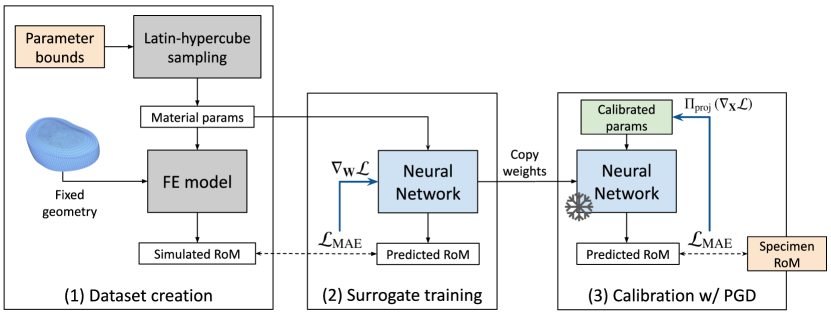
Figure 1: Calibrating an L4-L5 intervertebral disc (IVD) finite element (FE) model to match in vitro Range-of-Motion (RoM) measurements. (1) Create a dataset by sampling material parameters within feasible bounds using Latin hypercube sampling (LHS) [34] and obtaining corresponding RoM values with FE simulations. (2) Train a neural network (NN) surrogate to minimize the Mean Absolute Error (MAE) between the predicted and simulated RoM. (3) Freeze the network weights and optimize the NN input parameters to match the predicted RoM to the experimental measurements. Projected Gradient Descent (PGD) ensures the optimized parameters remain within feasible bounds.

We present a three-step method for calibrating an L4-L5 IVD FE model to match experimental Range-of-Motion (RoM) measurements (Fig. 1). First, we create a dataset using Latin hypercube sampling (LHS) [34] and generate corresponding FE simulation RoM outputs. Next, we train a surrogate NN model to approximate the FE model’s behavior, enabling efficient predictions. Finally, we calibrate the FE model to experimental measurements by optimizing the input parameters with PGD. During this calibration step, the weights of the pre-trained NN model are frozen, ensuring that only the inputs are adjusted and leveraging the surrogate’s learned representation.

We begin this section by describing the FE model and the dataset used for training the surrogate models. Afterward, we detail the surrogate model architectures and the training process. Finally, we explain the calibration process, including the optimization method and the baseline comparisons to a GA and an inverse model.

2.1 FE model and dataset

Let $\mathbf{p}_{i}=[p_{1},\ldots,p_{d}]\in\mathbb{R}^{d}$ represent a set of material configurations, where $d=13$ denotes the dimensionality of the parameter space and $1\leq i\leq n$ indexes the individual configurations. The configurations were sampled with LHS, thus ensuring a comprehensive exploration of the parameter ranges by dividing them into equally probable intervals. Each input parameter $p_{j}$ was restricted to a feasible range [30, forthcoming], as detailed in B.1. Subsequently, we experimented with surrogates trained on configuration sets of various sizes.

The sampled configurations $\mathbf{p}$, each comprising 13 model parameters, were used to perform simulations with an established FE model of the human L4-L5 IVD [7, 14]. Besides $\mathbf{p}$, the simulation inputs a Load Case definition specifying the direction and a Moment magnitude of the applied mechanical loading. Specifically, load cases $c\in(1,2,3,4)$ were used, representing axial rotation, extension, flexion, and lateral bending, as detailed by Heuer et al. [9]. For each load case, five different moment magnitudes $m\in(1,2,3,4,5)$, measured in Nm, were applied. The output of each simulation was the rotational displacement of the IVD, expressed as the RoM in degrees $r_{c,m}\in\mathbb{R}_{>0}$. This RoM represents the rotational change around the axis corresponding to the applied load case, measured relative to the initial position.

Figure 2: Meshed geometry of the L4-L5 IVD and the strain energy density functions in the FE model [7, 14]. The figure shows the separation into nucleus pulposus (gray) and annulus fibrosus (blue), both with hyperelastic material definitions. The strain energy density functions for the nucleus ($\mathit{W_{n}}$, Mooney-Rivlin) and annulus ($\mathit{W_{a}}$, Holzapfel-Gasser-Ogden) are provided, with the latter specifically accounting for the anisotropic properties of the annulus. The calibration process involved 13 parameters, with five in the strain energy density functions (bold). The remaining parameters, used in functions not provided here, describe fiber dispersion, angle variations, and stiffness changes across the annulus. For a more detailed explanation, refer to our previous publications [7, 14].

The IVD geometry used in the FE model (Fig. 2) was manually reconstructed based on average dimensions reported in the literature [14]. The model included a clear separation between the nucleus pulposus (gray) and the annulus fibrosus (blue), both defined with hyperelastic material properties. The Mooney-Rivlin material model ($\mathit{W_{n}}$) described the material behavior of the nucleus pulposus, while the Holzapfel-Gasser-Ogden material model ($\mathit{W_{a}}$) [35] was used for the annulus fibrosus to account for its anisotropic properties [8]. These strain energy density functions, $\mathit{W_{n}}$ and $\mathit{W_{a}}$, describe the energy stored in a material per unit volume during deformation [36]. The annulus fibrosus was segmented into five symmetrical subregions, each containing five layers to reflect radial differences in the material properties of the IVD. The modeling process, combined with the specific material parameters from the strain energy density functions, resulted in 13 different parameters characterizing the behavior of the FE model. The model was meshed using quadratic hexahedral elements.

The simulations were performed on an AMD Ryzen 7 7700X machine with an NVIDIA GeForce RTX 4090 GPU, averaging 208 seconds per simulation. Input configurations for which the FE simulation did not converge were removed from the dataset, and both input and output values were normalized to the range (0,1) with min-max normalization based on the defined parameter ranges.

2.2 Surrogate models

A surrogate ML model $\mathcal{M}$ was trained to predict a single RoM value $r_{c,m}\in\mathbb{R}^{0}$ for given material parameters $\mathbf{p}\in\mathbb{R}^{d}$ conditioned on a load case $c\in\mathbb{R}$ and a moment $m\in\mathbb{R}$. Formally, this is represented:

$$\mathcal{M}:[c,m,\mathbf{p}]\rightarrow r_{c,m}$$ (1)

Predicting a single RoM value for each load case and moment combination allows the model to more accurately capture the dependencies between material parameters and RoM.

Following the literature [15], we evaluated Linear Regression (LR), Support Vector Machine for Regression (SVR) [37], Random Forest (RF), Light Gradient-Boosting Machine (LightGBM) [38], Gaussian Process (GP), and NN surrogates. We used off-the-shelf implementations from scikit-learn [39] for LR, SVR, RF, and GP, and the official one for LightGBM [38]. The NN was implemented with PyTorch [40]. Hyperparameters for all models were searched with Optuna [41], with details provided in B.3. The models were trained and evaluated on the same machine mentioned before.

Neural network (NN)

We employed a simple feed-forward architecture for the NN consisting of five linear layers, each followed by a ReLU activation function. The final layer outputs the predicted RoM value and is not constrained to a specific range (e.g., (0,1)), allowing for extrapolation to unseen RoM values during calibration to some specimens. The loss function was the Mean Absolute Error (MAE) between the predicted and ground-truth RoM values.

The network weights were optimized using the Adam optimizer. An early stopping mechanism was incorporated to halt training if no improvement in the loss was observed over the validation set, preventing overfitting. We applied L2 regularization to the network’s weights to further mitigate overfitting and used Dropout [42], where randomly selected NN weights were zeroed during training. Dropout encourages the network to learn robust features and reduces dependency on any single neuron, enhancing generalization.

2.3 FE model calibration

The calibration process determines input parameters that match reported in vitro RoM measurements by minimizing the difference between the surrogate outputs and the measurements. The developed method utilized an optimization stirred with gradients from the NN surrogate model. We compared it to a GA [14], which used the NN’s output instead of the FE model’s (GA w/ NN) and a developed inverse model.

2.3.1 Projected Gradient Descent with NN (PGD w/ NN)

The pre-trained NN surrogate guides the search for input parameters $\mathbf{x}_{\text{cal}}\in\mathbb{R}^{d}$ to achieve desired RoM values $\mathbf{y}\in\mathbb{R}^{k}$ for all load cases and moments specified by an experimental measurement, i.e., $k=|LoadCases|\times|Moments|$. We employed Projected Gradient Descent (PGD) [43, p. 263] to optimize $\mathbf{x}_{\text{cal}}$ so that the network output matches $\mathbf{y}$. During this process, the NN weights were frozen and not changed, ensuring that the model’s learned representation remained consistent and that only the input parameters were adjusted. This process differs from the one used during the training phase of the NN, where the weights were updated to learn the mapping from inputs to outputs.

PGD is an optimization technique explicitly maintaining the feasibility of the solution in settings where traditional gradient descent may violate physical or practical constraints. It incorporates into gradient descent’s update step a projection function to ensure that the updated parameters remain within predefined constraints:

$$\mathbf{X}^{(t+1)}=\Pi_{\text{proj}}\left(\mathbf{X}^{(t)}-\eta\nabla_{\mathbf{X}^{(t)}}\mathcal{L}\right)$$ (2)

where $\eta$ is the learning rate, $\nabla_{\mathbf{X}}\mathcal{L}$ is the gradient of the loss function with respect to $\mathbf{X}$ and $\Pi_{\text{proj}}$ is a projection function (as described below). This explicit enforcement of constraints distinguishes our method from the approach by Maso Talou et al. [33], which used a penalty loss to implicitly encourage feasible solutions.

Input:

 $\mathbf{X}_{\text{search}}\in\mathbb{R}^{k\times(2+d)}$: Search matrix.

 $T$: Number of optimization steps.

 $\mathbf{NN}_{\text{{\char 94\relax}}}$: Pretrained NN with frozen weights.

 $\mathbf{y}\in\mathbb{R}^{k}$: Target specimen RoM column.

 $\eta$: Learning rate.

Output:

 $\mathbf{x}_{\text{cal}}\in\mathbb{R}^{d}$: Calibrated parameters

$\mathbf{X}^{(1)}\leftarrow\mathbf{X}_{\text{search}}$; // Initialize $\mathbf{X}$

for $t=1$ to $T$ do

       $\hat{\mathbf{y}}\leftarrow\mathbf{NN}_{\text{{\char 94\relax}}}\left(\mathbf{X}^{(t)}\right)$; // NN inference

       $\mathcal{L}_{\text{MAE}}\leftarrow\frac{1}{k}\sum_{i=1}^{k}\|\mathbf{y}_{i}-\hat{\mathbf{y}}_{i}\|_{1}$; // MAE loss

       $\mathbf{X}^{(t+1)}\leftarrow{\Pi}_{\text{proj}}\left(\mathbf{X}^{(t)}-\eta\cdot\nabla_{\mathbf{X}^{(t)}}\mathcal{L}\right)$; // Project optimized parameters

      

end for

$\mathbf{x}_{\text{cal}}\leftarrow\mathbf{X}^{(T)}_{0,}$; // Extract parameter values

return $\mathbf{x}_{\text{cal}}$

Algorithm 1 PGD w/ NN calibration

Alg. 1 provides an overview of the calibration process. It inputs the target RoM measurements $\mathbf{y}\in\mathbb{R}^{k}$ and a search matrix $\mathbf{X}_{\text{search}}\in\mathbb{R}^{k\times(2+d)}$, in which the first two columns are set to combinations of load cases $\mathbf{c}\in\mathbb{R}^{c}$ and moments $\mathbf{m}\in\mathbb{R}^{m}$, specifying the conditions for which the target RoM values $\mathbf{y}\in\mathbb{R}^{k}$ are given. The other $d$ columns are set with some random input vector $\textbf{x}_{init}\sim U(0,1)^{d}$.

In a loop, the NN infers RoM values $\hat{\mathbf{y}}$ for the current input, and an MAE loss for the ground-truth $\mathbf{y}$ is computed. Next, the gradient of the loss function with respect to the input $\nabla_{\mathbf{X}}\mathcal{L}$ is derived, and a PGD step is performed to update $\mathbf{X}$. These steps are performed only on the optimized parameters while leaving the first two columns of $\mathbf{X}$ intact to not change the condition load cases and moments. The process is repeated for $T$ steps until it converges. Finally, the calibrated parameter values $\mathbf{x}_{\text{cal}}$ are extracted from one of the rows of $\mathbf{X}$ (as all the rows are identical, details to follow) and returned.

The projection function operates as follows:

$$\Pi_{\text{proj}}\left(\mathbf{X}\right) =\mathbf{1}_{k}\cdot\text{ClipBounds}(\overline{\mathbf{x}})$$ (3)

$$\text{where}\quad\overline{\mathbf{x}} =\frac{1}{k}\sum_{k=1}^{k}\mathbf{X}_{k,},\quad\overline{\mathbf{x}}\in\mathbb{R}^{d},$$ (4)

$$\text{ClipBounds}(\mathbf{x}) =\min(\max(\mathbf{x},\mathbf{b}_{\text{min}}),\mathbf{b}_{\text{max}})$$ (5)

Initially (Eq. 4), it calculates the mean value across the rows of $\mathbf{X}$, thus ensuring a single candidate value per input parameter across all load cases and moments. Then (Eq. 5), it enforces predefined constraints by clipping the values within the bounds $\mathbf{b}_{\text{min}},\mathbf{b}_{\text{max}}\in\mathbb{R}^{d}$. These bounds are the same as those used for sampling the training dataset in Sec. 2.1. Finally (Eq. 3), it inflates the result back to a matrix form by multiplying it from the left with a vector of $k$ ones $\mathbf{1}_{k}$, thus creating a matrix of $k$ identical rows. Fig. 3 further illustrates this projection process.

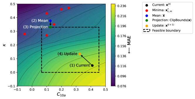
Figure 3: Illustration of Projected Gradient Descent (PGD) in the loss landscape of two calibrated parameters. The contour plot shows the RoM MAE between the surrogate NN’s predictions and the third specimen by Nicolini et al. [44]. Only two input parameters are varied for illustration, while the others are fixed. The dashed box represents the feasible input parameter area. The algorithm follows these steps: (1) It starts from the black point, indicating the current step’s configuration. (2) Using gradients of the loss, the red points representing local minima for specific load case and moment combinations are obtained, and their mean is computed, shown by the blue point. (3) This mean is then projected into the feasible area, shown by the green point. (4) Finally, the algorithm updates the configuration toward the projection, leading to the orange point, with the step size depending on the learning rate.

In practice, Alg. 1 was run $M=500$ times with different random initialization of $\mathbf{x}_{\text{init}}$ set into $\mathbf{X}_{\text{search}}$ and the best solution in terms of $\overline{\mathcal{R}^{2}}$ score across the different load cases was chosen. The multiple runs did not affect the overall search time, as the algorithm was implemented to perform all optimization rounds in parallel. The hyperparameters $\eta$, $T$ and $M$ were chosen using Optuna [41]. We used the Adam optimizer in Eq. 2 instead of a vanilla Gradient Descent for improved results.

2.3.2 Calibration baselines

GA w/ NN

We employed a GA [7, 14] as a first baseline, substituting the FE model in the original works with the NN surrogate. We opted for this approach because running the calibration without the surrogate would be infeasible due to the excessive running time. We used the settings from the original works [7, 14] while restricting the sampled parameters bounds as described previously and increasing the $\overline{\mathcal{R}^{2}}$ stopping criteria to 1. We increased this criteria for fairer comparison with the developed method and since using the surrogate circumvents previous computational restrictions. Additional details are provided in B.2.

Inverse model

Following the approach of [28, 29], we developed a model to predict material parameters from an input vector of RoM values. The training setup is thus inverse to the one used for the surrogates:

$$\mathcal{M}_{Inverse}:[r_{1,1},..,r_{1,5},..,r_{4,1},..,r_{4,5}]\rightarrow\mathbf{p}$$ (6)

where $\mathcal{M}_{Inverse}$ is an ML model, $\mathbf{p}\in\mathbb{R}^{d}$, and $r_{c,m}\in\mathbb{R},\forall c\in(1,2,3,4)$, $\forall m\in(1,2,3,4,5)$ as defined in Sec. 2.1. Notably, $\mathcal{M}_{Inverse}$ was not conditioned on specific $c$ and $m$ as the surrogate models in Eq. 1; instead, all RoM values were provided to give complete context for inferring $\mathbf{p}$.

In order to obtain a dataset for training the inverse model, we sampled random material configurations $\mathbf{p}$ within the material bounds as before and inferred their corresponding RoM values for all load cases and moments using the NN surrogate. We then trained an NN model in this inverse setting. Additional details are provided in B.2.

2.4 Evaluation metrics

We evaluated the surrogate models and the calibration methods using the Mean Absolute Error (MAE), commonly used to evaluate regression problems. The MAE between the ground truths RoM $y$ and the outputs $\hat{y}$ is averaged over load cases and moments as follows:

MAE $$=\frac{\sum_{c\in\text{LoadCases}}{\sum_{m\in\text{Moments}}{|y_{c,m}-\hat{y}_{c,m}|}}}{|\text{LoadCases}|\times|\text{Moments}|}$$ (7)

For the surrogate models, the ground truth $y$ is the FE numerical simulation result, and the output $\hat{y}$ is the surrogate predicted value. For the calibration methods, the ground truth $y$ is the experimental measurement, and the output $\hat{y}$ is the FE numerical result for the calibrated configuration.

Additionally, we used the mean $\mathcal{R}^{2}$-score, denoted $\overline{\mathcal{R}^{2}}$, which measures the proportion of variance explained across different load cases [45, 8]:

$$\overline{\mathcal{R}^{2}} =\frac{\sum_{c\in\text{LoadCases}}{\mathcal{R}^{2}_{c}}}{|\text{LoadCases}|}$$ (8)

$$\text{where}\ \forall c\in\text{LoadCases},\quad\mathcal{R}^{2}_{c} =1-\frac{\sum_{m\in\text{Moments}}{\left(y_{c,m}-\hat{y}_{c,m}\right)^{2}}}{\sum_{m\in\text{Moments}}{\left(y_{c,m}-\overline{y_{c}}\right)^{2}}}$$ (9)

where $\overline{y_{c}}$ is the mean of the ground truths across moments for load case $c$.

3 Results and discussion

This section compares the performance of the different surrogate models used to approximate FE model simulations. Then, we discuss the results of the calibration methods by evaluating them on both synthetic and experimental data. Finally, we conduct ablation studies to understand the impact of various components of our approach. Additional results are provided in C.

3.1 Surrogate models

To enhance the efficiency and accuracy of FE calibration, we explore using surrogate models as a faster and more reliable alternative to direct simulations. This section assesses the performance of various surrogate models, focusing on the effects of training dataset size and model architecture. Additionally, it investigates the models’ ability to interpolate and extrapolate RoM values to unseen moments, which is essential for calibrating to experimental data.

3.1.1 Training set size and model architecture

The size of the dataset used for training surrogate models is critical due to the time-consuming nature of FEM simulations. Table 1 explores the number of samples required for accurate model predictions, comparing datasets of 128, 512, and 1024 samples, all generated using LHS. The models were evaluated on a test set of 64 randomly sampled configurations. All ground-truth RoM values were obtained by running FE simulations, and all experiments were conducted with 4-fold cross-validation.

Table 1: Mean $\overline{\mathcal{R}^{2}}$ (higher is better) and MAE (lower is better) scores for surrogates trained on different dataset sizes, with standard deviations on cross-validated folds. Also shown is the time required to create each dataset.

Surrogate model	$n=128$		$n=512$		$n=1024$
	$\overline{\mathcal{R}^{2}}$ $\uparrow$	MAE $\downarrow$	$\overline{\mathcal{R}^{2}}$ $\uparrow$	MAE $\downarrow$	$\overline{\mathcal{R}^{2}}$ $\uparrow$	MAE $\downarrow$
Logistic Regression (LR)	0.55$\pm$0.13	1.03$\pm$0.29	0.54$\pm$0.15	1.05$\pm$0.26	0.55$\pm$0.15	1.05$\pm$0.26
Support Vector Regression (SVR)	0.59$\pm$0.11	1.05$\pm$0.15	0.65$\pm$0.13	0.98$\pm$0.14	0.51$\pm$0.25	1.04$\pm$0.06
Random Forest (RF)	0.82$\pm$0.03	0.65$\pm$0.17	0.89$\pm$0.06	0.46$\pm$0.16	0.91$\pm$0.04	0.40$\pm$0.12
Gaussian Process (GP)	0.83$\pm$0.04	0.62$\pm$0.18	0.92$\pm$0.01	0.43$\pm$0.09	0.95$\pm$0.01	0.33$\pm$0.09
LightGBM	0.85$\pm$0.01	0.57$\pm$0.12	0.95$\pm$0.02	0.34$\pm$0.09	0.96$\pm$0.01	0.28$\pm$0.07
Neural Network (NN)	0.90$\pm$0.02	0.43$\pm$0.12	0.98$\pm$0.00	0.16$\pm$0.04	0.99$\pm$0.00	0.10$\pm$0.03
Elapsed simulation time (hours)	29.6		118.4		236.9

As shown in Table 1, increasing the dataset size significantly improves most models. For instance, the RF model’s MAE decreases from 0.65 to 0.40 as the dataset grows from 128 to 1024, demonstrating that larger datasets help models capture underlying patterns more effectively. Simpler models like LR and SVR struggle with the non-linear interactions in the FE simulation [7], resulting in poor performance with MAEs of 1.05 and 1.04, respectively, even when trained on 1024 samples. This makes them less suitable for accurate predictions in this context. The NN model considerably improves, achieving an MAE of 0.10 and $\overline{\mathcal{R}^{2}}$ of 0.99 for 1024 samples. Notably, the NN model’s MAE of 0.43 for 128 samples may already be sufficient for some applications, requiring only about 30 hours to create the dataset. Observing that the NN surrogate begins to converge at 512 samples, we selected the best-performing NN model, trained on 1024 samples, for all subsequent experiments.

3.1.2 Interpolation and extrapolation

The ability to interpolate and extrapolate to unseen moments is crucial for the developed calibration method, as it relies on surrogate models and experimental measurements that are often reported at moments different from those used for training the surrogate. These generalization abilities are evaluated in Fig. 4, where the top four performing surrogate models are tested on a dataset of 64 synthetic configurations with ground-truth RoM values for moments in the range (0.5, 10) Nm at 0.5 intervals. The evaluation assesses performance on moments on which the model was trained (1, 2, 3, 4, 5), interpolated moments (1.5, 2.5, 3.5, 4.5), and extrapolated moments (0.5 and $>5$). Cross-validated results are provided in Table 2.

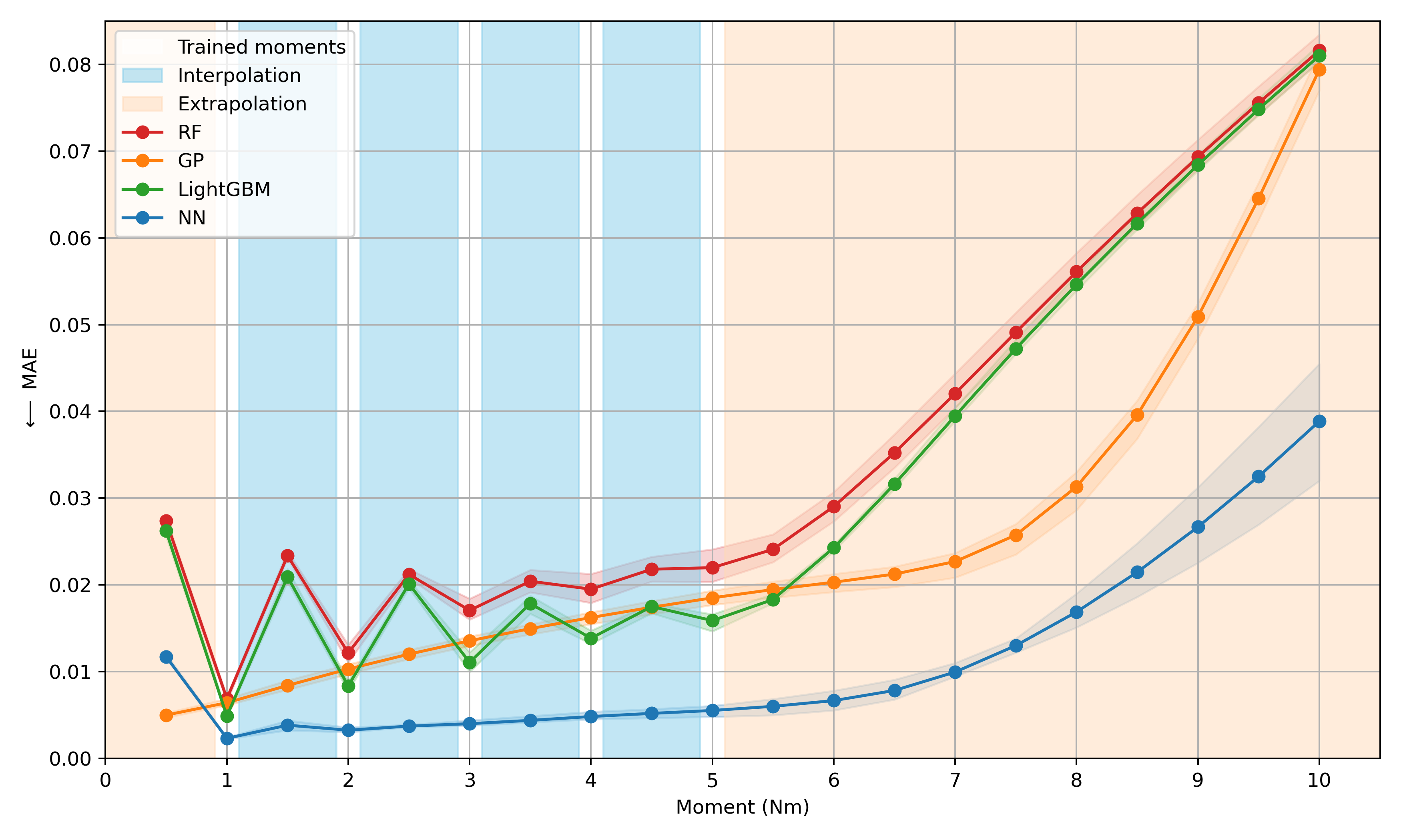
Figure 4: Interpolation and extrapolation abilities of surrogate models across moments. The background colors correspond to the ranges evaluated: white for trained moment, peach for extrapolation, and blue for interpolation. Both abilities are essential for the calibration of specimens. The line shadings represent the standard deviation across the cross-validated folds. The NN surrogate outperforms the other models for all but moments of 0.5 Nm.

Decision tree-based methods, specifically RF and LightGBM, perform well on trained moments but struggle with unseen ones, indicating limited generalization ability. Interestingly, the GP model excels at a moment of 0.5 Nm with an MAE of 0.005, but this is insignificant since low-moment experimental measurements are uncommon. However, the GP also shows a significant performance drop for moments greater than 6 Nm. The NN model demonstrates superior performance across all moments above 1 Nm, achieving the lowest MAE of 0.004 on trained and interpolated moments. However, it shows increased error and variability for extremely high moments, indicating that while the NN surrogate is highly effective, it may still face challenges with extensive extrapolation.

Table 2: Comparison of interpolation and extrapolation ability of the top performing surrogate models. The row colors match those of Fig. 4: white for trained moments, peach for moment extrapolation, and blue for moment interpolation. The results are the mean and standard deviation across the folds.

Moments (Nm)	Random Forest (RF)		Gaussian Process (GP)		LightGBM		Neural Network (NN)
	$\overline{\mathcal{R}^{2}}$ $\uparrow$	MAE $\downarrow$	$\overline{\mathcal{R}^{2}}$ $\uparrow$	MAE $\downarrow$	$\overline{\mathcal{R}^{2}}$ $\uparrow$	MAE $\downarrow$	$\overline{\mathcal{R}^{2}}$ $\uparrow$	MAE $\downarrow$
1, 2, 3, 4, 5	0.92$\pm$0.01	0.01$\pm$0.00	0.95$\pm$0.00	0.01$\pm$0.00	0.96$\pm$0.00	0.01$\pm$0.00	0.99$\pm$0.00	0.00$\pm$0.00
0.5	-2.10$\pm$0.12	0.03$\pm$0.00	0.85$\pm$0.01	0.00$\pm$0.00	-1.85$\pm$0.18	0.03$\pm$0.00	0.43$\pm$0.01	0.01$\pm$0.00
1.5, 2.5, 3.5, 4.5	0.87$\pm$0.01	0.02$\pm$0.00	0.95$\pm$0.00	0.01$\pm$0.00	0.91$\pm$0.01	0.02$\pm$0.00	0.99$\pm$0.00	0.00$\pm$0.00
$>5$	0.69$\pm$0.02	0.05$\pm$0.00	0.82$\pm$0.01	0.04$\pm$0.00	0.73$\pm$0.01	0.05$\pm$0.00	0.95$\pm$0.01	0.02$\pm$0.00

3.2 FE model calibration

In this section, the performance of the proposed calibration method is compared to the baselines. First, we test the calibration methods on a synthetic dataset to establish baseline performance and computational efficiency. We apply the calibration techniques to in vitro experimental measurements from Nicolini et al. [44] and Heuer et al. [9], assessing their practical applicability and robustness.

3.2.1 Synthetic data

We evaluated the calibration methods using a synthetic test set of 64 sampled configurations. Each method received target RoM values for the four load cases at the five moments and was tasked with predicting the corresponding configuration parameter values. The predicted configurations were then input into the surrogate to assess the agreement between the predicted and target RoM values. Due to the considerable running time of the FE for 64 samples, we did not validate these results with simulations.

Table 3: Comparison of calibration methods on synthetic data, with mean and standard deviation across the test set. The evaluation is performed on the moments predicted by the surrogate for the found configurations. Calibration time on the entire test set is provided.

Load case	PGD w/ NN (Ours)		GA w/ NN		Inverse model
	$\mathcal{R}^{2}$ $\uparrow$	MAE $\downarrow$	$\mathcal{R}^{2}$ $\uparrow$	MAE $\downarrow$	$\mathcal{R}^{2}$ $\uparrow$	MAE $\downarrow$
Axial Rotation	0.99$\pm$0.01	0.07$\pm$0.06	0.93$\pm$0.08	0.21$\pm$0.18	-0.04$\pm$1.57	0.80$\pm$0.73
Extension	0.98$\pm$0.12	0.07$\pm$0.18	0.95$\pm$0.06	0.24$\pm$0.20	0.61$\pm$0.73	0.59$\pm$0.46
Flexion	1.00$\pm$0.00	0.05$\pm$0.03	0.97$\pm$0.05	0.17$\pm$0.14	0.82$\pm$0.20	0.41$\pm$0.28
Lateral Bending	1.00$\pm$0.01	0.04$\pm$0.04	0.98$\pm$0.02	0.09$\pm$0.06	0.78$\pm$0.28	0.27$\pm$0.20
Mean	0.99$\pm$0.01	0.06$\pm$0.02	0.96$\pm$0.05	0.18$\pm$0.13	0.54$\pm$0.34	0.52$\pm$0.20
Total running time (seconds)	2.58		11.92		0.01

Table 3 demonstrates that PGD w/ NN outperforms both baselines on synthetic data, achieving the lowest MAE of 0.06 and an $\overline{\mathcal{R}^{2}}$ score of 0.99, with a runtime of approximately 2.6 seconds. The GA w/ NN method also performs well, with an MAE of 0.18 and $\overline{\mathcal{R}^{2}}$ of 0.96, but it exhibits a more considerable variability across moments for most load cases. The high performance of both methods is expected since the calibrated target RoM values were derived from the same FE model used to create the training dataset. Though the inverse model is the fastest, requiring only 0.01 seconds, it fails to obtain applicable configurations, yielding a mean MAE of 0.52 and $\overline{\mathcal{R}^{2}}$ of 0.54. The primary issue is the ill-posedness of the inverse setting [46], where numerous, very different configurations can result in almost identical RoM measurements. Due to this lack of convergence, we did not evaluate the inverse model on experimental data.

3.2.2 Experimental specimen

To asses their relevance to real-world problems, we evaluated the calibration methods on six in vitro experimental specimens. We used five specimens reported by Nicolini et al. [44] in the same conditions used to train the surrogate. Additionally, a mean of eight specimen measurements reported by Heuer et al. [9] was utilized and preprocessed as suggested by Gruber et al. [14]. This measurement is available at moments different from the ones for which the surrogate was trained. Each method was given the target RoM values and tasked with predicting the corresponding configurations. Different from before, these predicted configurations were then validated with FE simulations to assess the agreement between the simulated and target RoM.

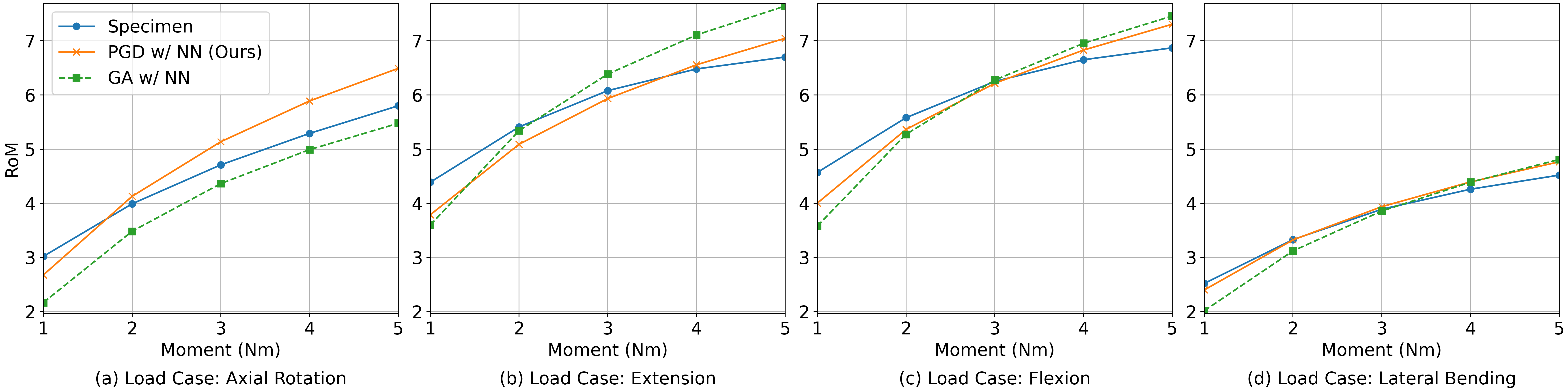
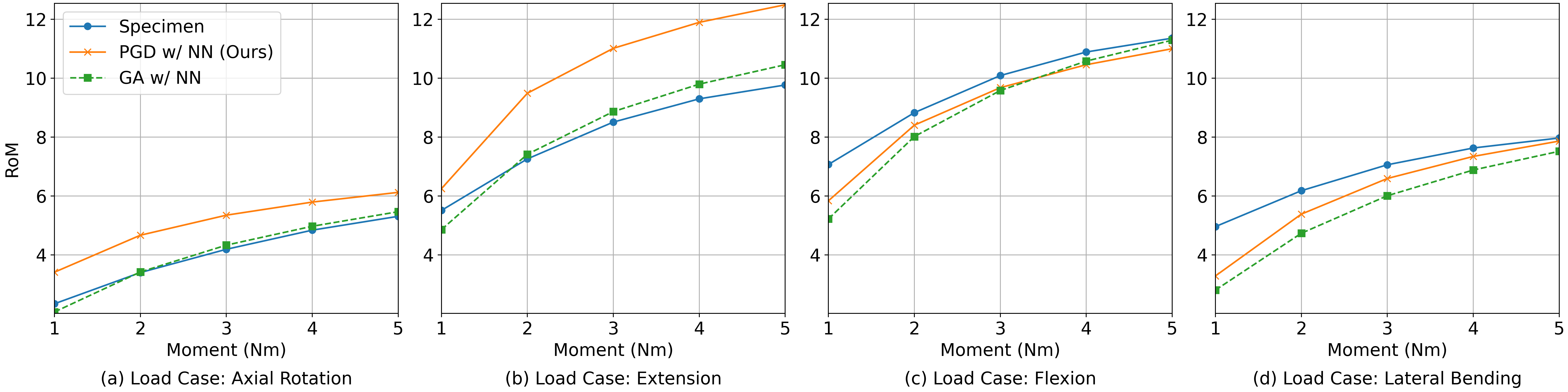
Figure 5: Example calibration results for samples 1 (top) and 3 (bottom) from Nicolini et al. [44]. The plots show the RoM values for the in vitro measurements (blue), the calibrated configuration using the proposed method (orange), and the GA w/ NN baseline (green). The proposed method performs better on sample 1 than sample 3. The poorer performance on sample 3 is attributed to the large variability in RoM across load cases in the target configuration, which differs significantly from the surrogate’s training data. Results for the other specimens are in C.

Detailed examples are shown in Fig. 5 and Table 4 summarizes the results. The GA baseline required up to 47 generations to converge on the specimens (see C). Notably, running the GA with FE simulations instead of the NN surrogate on the same machine would have taken up to 8 days per specimen for comparable results to our method, which is impractical for this study’s time constraints.

Table 4: Comparison of calibration methods on experimental specimens, showing the mean and standard deviation across load cases per sample.

Sample		PGD w/ NN (Ours)		GA w/ NN
		$\overline{\mathcal{R}^{2}}$ $\uparrow$	MAE $\downarrow$	$\overline{\mathcal{R}^{2}}$ $\uparrow$	MAE $\downarrow$
Nicolini et al. [44]	1	0.97 $\pm$ 0.02	0.28 $\pm$ 0.13	0.95 $\pm$ 0.01	0.42 $\pm$ 0.13
	2	0.96 $\pm$ 0.07	0.07 $\pm$ 0.04	0.97 $\pm$ 0.02	0.10 $\pm$ 0.08
	3	0.80 $\pm$ 0.17	1.11 $\pm$ 0.72	0.93 $\pm$ 0.08	0.62 $\pm$ 0.43
	4	0.91 $\pm$ 0.07	0.35 $\pm$ 0.13	0.93 $\pm$ 0.03	0.37 $\pm$ 0.16
	5	0.94 $\pm$ 0.08	0.20 $\pm$ 0.21	0.94 $\pm$ 0.05	0.27 $\pm$ 0.14
Heuer et al. [9]	Mean	0.97 $\pm$ 0.02	0.41 $\pm$ 0.29	0.95 $\pm$ 0.03	0.55 $\pm$ 0.31

Optimizing for MAE

The proposed method shows increased performance in MAE, outperforming the baseline on five out of six specimens. However, it exceeds the baseline in $\overline{\mathcal{R}^{2}}$ for only three of the six samples, which aligns with the optimization’s focus on minimizing MAE. Notably, for the third sample by Nicolini et al. [44], our method’s MAE is higher than the baseline’s (1.11 vs. 0.62). Both methods performed well for the mean of specimens by Heuer et al. [9] (MAE of 0.41 and 0.55, respectively), leveraging the surrogate’s interpolation and extrapolation capabilities (Sec. 3.1.2).

Increased error at lowest and highest moment

Fig. 6 analyzes the error values across moments, averaged across load cases for experimental data. A significant increase in error is apparent at the lowest moment for many specimens. However, the surrogate evaluation in Sec. 3.1.2 suggests this error does not originate from the surrogate itself. An increase in error is also noticeable at the highest moment. We hypothesize that many measurements, such as the first sample by Nicolini et al. [44], exhibit high non-linearity, particularly in the transition between 1 and 2 Nm. This high non-linearity challenges the underlying FE model, producing poorer calibration results. Observations about the difficulties of this FE model in capturing diverse specimens while assuming identical geometry were reported by Nicolini et al. [44, 7].

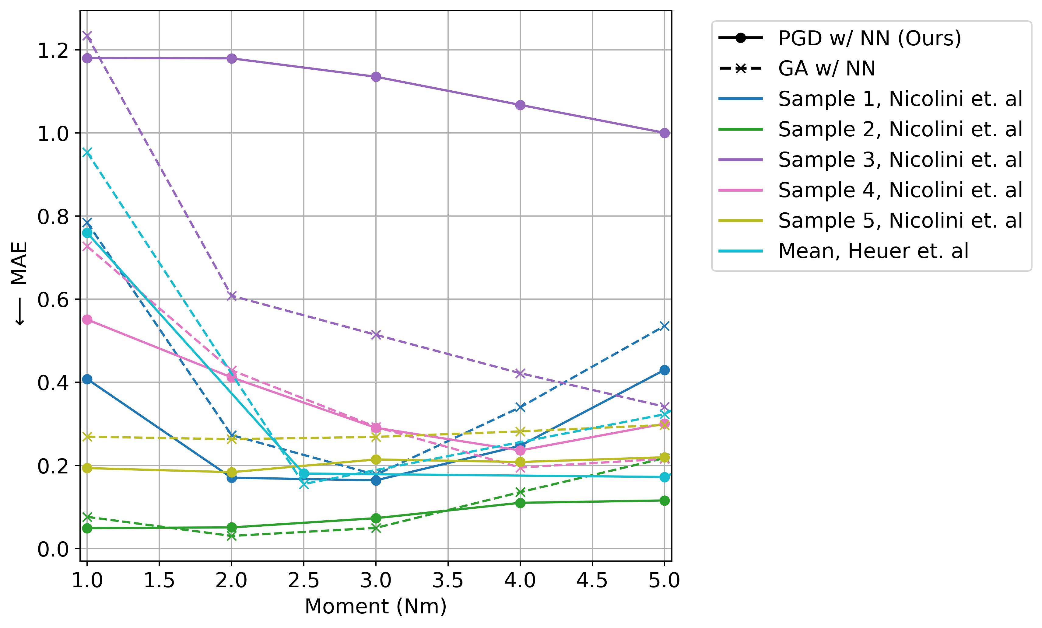
Figure 6: Comparison of MAE vs. moment averaged across load cases on experimental specimens. Specimens are color-coded. The proposed method outperforms the baseline except for the third sample from Nicolini et al. [44] (purple). Both methods present an increased error at the lowest and highest moments.

Sensitivity to high variability in moment magnitude

Table 4 highlights challenges with the third sample from Nicolini et al. [44], which we attribute to significant variations in target RoM magnitudes. Fig. 7 presents matrices of absolute RoM differences. Each cell shows the absolute difference between a specific RoM value and the corresponding values for the same sample across the other load cases. These matrices provide a detailed comparison of how the RoM varies between different conditions for each sample. Notably, the third sample (Fig. 7(b), right cell split) has much higher differences in axial rotation and flexion (4.4 and 3.7, respectively) compared to other test specimens (Fig. 7(b), left cell split) and the surrogate’s training set (Fig. 7(a)).

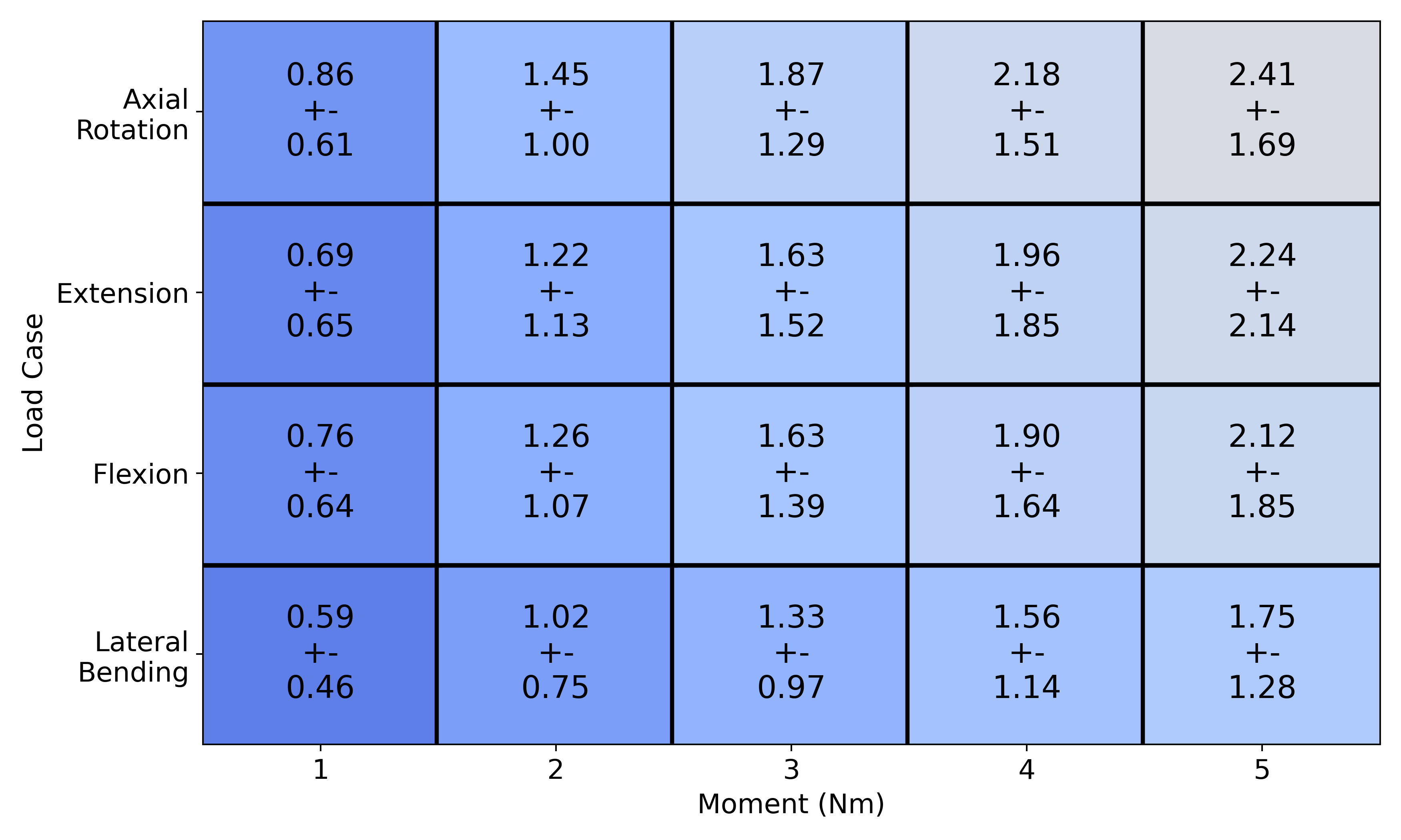
(a)

(b)

Figure 7: Matrix comparison of absolute differences in RoM across load cases. Each cell presents the difference between a specific RoM value and the values for the same sample at the same moment for other load cases. The left (a) shows the differences for the training set. The right (b) displays the differences for experimental values from Nicolini et al. [44], with the left cell split representing all samples except the third, and the right split showing only the third sample. For multiple samples, the mean and standard deviation are shown. Notably, the third sample by Nicolini et al. [44] exhibits significantly higher differences in axial rotation and flexion.

We hypothesize that this substantial variability in experimental data negatively impacts the optimization process. The GA w/ NN baseline, better suited for global optimization [47], excels in exploring a wider search space and finding configurations outside the training distribution. However, it still required five times more generations to converge for the third sample from Nicolini et al. [44] compared to the other specimens. In contrast, our method relies on NN weights derived from the training set, which do not account for such extreme configurations.

3.2.3 Ablation studies

To thoroughly analyze the proposed calibration method, ablation studies were performed using the experimental specimens by Nicolini et al. [44]. These studies focused on the impact of the projection step, loss function, and optimizer on calibration performance. Table 5 compares the evaluated settings and includes a final column summing parameter values exceeding physical bounds, with values above zero indicating infeasible solutions. Ablation of the NN model’s basic components (e.g., number of layers, activation function) was also conducted but not listed here.

The results demonstrate that the projection step is essential for ensuring feasible calibration outcomes. In the “Adam, L1 loss” setting, while the $\overline{\mathcal{R}^{2}}$ is highest at 0.95 and the MAE is lowest at 0.04, it results in a sum of 118.38 parameter values exceeding the bounds, making them infeasible for FE model input. With projection applied (“Adam, L1 loss, projection (Ours)”), the exceeding values drop to zero, though with a slight decrease in performance metrics ($\overline{\mathcal{R}^{2}}$ of 0.85 and MAE of 0.21).

Table 5: Ablation studies of the proposed calibration method, evaluated on the specimens by Nicolini et al. [44]. The last column sums the values exceeding the material bounds, with positive values representing infeasible solutions.

Optimization setting	$\overline{\mathcal{R}^{2}}$  $\uparrow$	MAE  $\downarrow$	Sum exceeding values  $\downarrow$
Adam, L1 loss	0.95	0.04	118.38
Adam, L1+bounds loss	0.86	0.21	0.11
Adam, L1 loss, projection (Ours)	0.85	0.21	0
Adam, L2 loss, projection	0.84	0.25	0
L-BFGS, L1 loss, projection	-1.0	0.93	0

The “Adam, L1+bounds loss” setting, incorporating a penalty for out-of-bound values similar to Maso Talou et al. [33], reduces infeasible values to 0.11. However, it does not eliminate them, rendering some results unusable for the FE model. Not listed here, higher penalty weights reduced exceeding values but significantly degraded performance. Using an L2 loss (“Adam, L2 loss, projection”) treats large errors more severely, encouraging the minimization of significant deviations. An NN surrogate trained with L2 loss was used for consistency in this setting. However, this loss performed slightly worse than L1 loss, with an $\overline{\mathcal{R}^{2}}$ of 0.84 and an MAE of 0.25. Lastly, following Maso Talou et al. [33], we tried the L-BFGS optimizer instead of Adam. The “L-BFGS, L1 loss, projection” setting performed poorly, with an $\overline{\mathcal{R}^{2}}$ of -1.0 and an MAE of 0.93, indicating that this optimizer is unsuitable for this task.

4 Conclusions and outlook

This study introduced a novel calibration method for an FE model of the human L4-L5 IVD guided by an NN surrogate. Using an NN surrogate provides near-instant predictions, allowing for rapid calibration through optimization with PGD. Additionally, incorporating the projection step ensures optimized parameter values remain within feasible bounds, addressing a potential pitfall in existing NN surrogate optimization-based calibration methods. This balance between performance and feasibility is crucial for practical applications in clinical settings. Moreover, the developed method outperformed the evaluated baselines. While the GA w/NN baseline was effective, it required more time and relied on an external algorithm. Despite its rapid inference, the inverse model struggled with ill-posedness, failing to produce useful material configurations.

However, the study revealed limitations in our approach and the underlying FE model. The high variability in moment magnitude among certain experimental specimens led to sub-optimal convergence, as the NN surrogate was not trained on such extremes. Augmenting the training dataset with more diverse cases could enhance robustness. Future work should focus on generating representative samples using active learning [48], which involves selectively querying the FE model to include challenging, real-world scenarios. Furthermore, incorporating varying geometric parameters as FE model inputs, rather than fixed average dimensions, could allow surrogate models to be used for patient-specific simulations, resulting in more accurate calibration and considerable applicability. Another potential extension is adapting the surrogate model for a multi-body environment, as suggested by Hammer et al. [17].

Data availability

The data used to train the surrogate models and the synthetic data used for evaluation are available in our GitHub repository. The experimental data used to evaluate the calibration methods could be obtained by contacting the respective authors.

Declaration of generative AI and AI-assisted technologies in the writing process

During the preparation of this work the the authors used ChatGPT and Grammarly to improve the readability and language of the manuscript. After using these tools, the authors reviewed and edited the content as needed and take full responsibility for the content of the published article.

Appendix A Mathematical notation

• Scalars, Vectors and Matrices:

  • $x\in\mathbb{R}$: A scalar.

  • $\mathbf{y}\in\mathbb{R}^{d}$: A vector of dimension $d$.

  • $\mathbf{X}\in\mathbb{R}^{n\times m}$: A matrix with $n$ rows and $m$ columns.

• Indices and Elements:

  • $\mathbf{x}_{i}$: The $i$-th element of the vector $\mathbf{x}$.

  • $\mathbf{X}_{i,j}$: The element in the $i$-th row and $j$-th column of the matrix $\mathbf{X}$.

  • $\mathbf{X}_{i,:},\mathbf{X}_{:,j}$: The $i$-th row of the matrix $\mathbf{X}$ and the $j$-th column of the matrix $\mathbf{X}$ respectively.

• Gradient and Partial Derivatives:

  • $\nabla_{\mathbf{X}}\mathcal{L}$: The matrix of partial derivatives of the scalar loss function $\mathcal{L}$ with respect to each element of the matrix $\mathbf{X}$.

Appendix B Detailed methodological parameters and models

B.1 Material parameters

Table 6: Material parameter ranges

Material Parameter	Minimum Value	Maximum Value
$C_{10n}$	0.03	0.21
$C_{01n}$	0.0075	0.0525
$C_{10a}$	0.065	0.455
$k_{1}$	1	50
$k_{2}$	10	200
$\kappa$	0	0.33
$k_{1c}$	-0.2	0
$k_{2c}$	-0.2	0
$k_{1r}$	-0.2	0
$k_{2r}$	-0.2	0
$\alpha$	7.5	52.5
$\alpha_{c}$	0	0.3
$\alpha_{r}$	0	0.2

B.2 Calibration baselines

GA

The GA [7, 14] was configured with a population size of 20, evolving from initially sampled random configurations within the parameter ranges. The six best-performing individuals from each generation are selected for Crossover and Mutation. During Crossover, four new individuals are created by combining pairs of the selected individuals. Mutation generates four new individuals by randomly altering a parameter of one of the selected individuals. Additionally, Immigration is performed, introducing six new individuals per generation. The process iterates until an $\overline{\mathcal{R}^{2}}=1$ stopping criteria is met or $100$ generations are reached.

Inverse model

The inverse NN was a five-layer feed-forward network with ReLU activation functions. Output values were constrained to (0,1) using a Sigmoid function and compared to ground truths with an MAE loss. An optimizer scheduler reduced the learning rate when the loss stopped improving on the validation set, enhancing training efficiency and convergence. We trained the network on a dataset of $50,000$ samples and, as before, implemented it with PyTorch. Hyperparameters are provided in B.3.

B.3 Models hyperparameters

Table 7: Hyperparameters used for training the ML models

Model	Hyper-parameters
LR	Default settings
RF	max_depth=31, n_estimators=51,
SVR	C=2.479459357922161, gamma=”auto”, kernel=”rbf”
LightGBM	num_leaves=71, max_depth=24, learning_rate=0.0959080973897064, n_estimators=183
GP	kernel=C(constant_value=1.3535458162698054e-05) RBF(length_scale=0.9739157609228299), normalize_y=True
NN (n=1024, n=512)	batch_size=20, layers_width=[256, 128, 64, 32, 16], learning_rate=0.000555, num_epochs=300, weight_decay=5.16293e-06, early_stopping_patience=23 dropout_probability=0.01
NN (n=128)	batch_size=14, layers_width=[128, 64, 32, 16, 8], learning_rate=0.000559, num_epochs=231, weight_decay=5.16442e-06, early_stopping_patience=26 dropout_probability=0.01
Inverse NN	batch_size=48, layers_width=[128, 256, 256, 256, 128], learning_rate=0.000654, num_epochs=776, weight_decay=0.000006, early_stopping_patience=50 dropout_probability=0.028433, scheduler=”ReduceLROnPlateau”, scheduler_patience=18, scheduler_factor=0.05

Appendix C Detailed results

Table 8: Surrogate models cross-validated $\mathcal{R}^{2}$ and MAE results. Training set $n=128$.

Model	Axial Rotation		Extension		Flexion		Lateral Bending		Mean
	$\mathcal{R}^{2}$ $\uparrow$	MAE $\downarrow$	$\mathcal{R}^{2}$ $\uparrow$	MAE $\downarrow$	$\mathcal{R}^{2}$ $\uparrow$	MAE $\downarrow$	$\mathcal{R}^{2}$ $\uparrow$	MAE $\downarrow$	$\mathcal{R}^{2}$ $\uparrow$	MAE $\downarrow$
LR	0.52$\pm$0.02	1.25$\pm$0.03	0.42$\pm$0.02	1.39$\pm$0.03	0.77$\pm$0.01	0.71$\pm$0.02	0.51$\pm$0.02	0.78$\pm$0.02	0.55$\pm$0.13	1.03$\pm$0.29
SVR	0.66$\pm$0.01	1.07$\pm$0.02	0.67$\pm$0.04	1.28$\pm$0.06	0.65$\pm$0.01	0.95$\pm$0.03	0.41$\pm$0.16	0.90$\pm$0.15	0.59$\pm$0.11	1.05$\pm$0.15
RF	0.78$\pm$0.03	0.80$\pm$0.04	0.84$\pm$0.03	0.78$\pm$0.05	0.82$\pm$0.01	0.65$\pm$0.01	0.86$\pm$0.02	0.36$\pm$0.02	0.82$\pm$0.03	0.65$\pm$0.17
GP	0.76$\pm$0.03	0.79$\pm$0.05	0.84$\pm$0.01	0.75$\pm$0.03	0.84$\pm$0.02	0.56$\pm$0.02	0.87$\pm$0.01	0.35$\pm$0.01	0.83$\pm$0.04	0.62$\pm$0.18
LightGBM	0.83$\pm$0.03	0.66$\pm$0.05	0.87$\pm$0.02	0.68$\pm$0.06	0.85$\pm$0.02	0.58$\pm$0.02	0.85$\pm$0.04	0.37$\pm$0.04	0.85$\pm$0.01	0.57$\pm$0.12
NN	0.86$\pm$0.02	0.58$\pm$0.05	0.91$\pm$0.02	0.50$\pm$0.03	0.91$\pm$0.01	0.39$\pm$0.01	0.93$\pm$0.02	0.25$\pm$0.03	0.90$\pm$0.02	0.43$\pm$0.12

Table 9: Surrogate models cross-validated $\mathcal{R}^{2}$ and MAE results. Training set $n=512$.

Model	Axial Rotation		Extension		Flexion		Lateral Bending		Mean
	$\mathcal{R}^{2}$ $\uparrow$	MAE $\downarrow$	$\mathcal{R}^{2}$ $\uparrow$	MAE $\downarrow$	$\mathcal{R}^{2}$ $\uparrow$	MAE $\downarrow$	$\mathcal{R}^{2}$ $\uparrow$	MAE $\downarrow$	$\mathcal{R}^{2}$ $\uparrow$	MAE $\downarrow$
LR	0.47$\pm$0.02	1.32$\pm$0.02	0.51$\pm$0.01	1.29$\pm$0.01	0.80$\pm$0.00	0.72$\pm$0.02	0.40$\pm$0.03	0.88$\pm$0.03	0.54$\pm$0.15	1.05$\pm$0.26
SVR	0.67$\pm$0.02	1.02$\pm$0.04	0.77$\pm$0.01	1.19$\pm$0.03	0.71$\pm$0.01	0.87$\pm$0.02	0.44$\pm$0.06	0.82$\pm$0.06	0.65$\pm$0.13	0.98$\pm$0.14
RF	0.79$\pm$0.02	0.69$\pm$0.02	0.94$\pm$0.01	0.48$\pm$0.03	0.90$\pm$0.01	0.45$\pm$0.01	0.94$\pm$0.01	0.23$\pm$0.01	0.89$\pm$0.06	0.46$\pm$0.16
GP	0.91$\pm$0.01	0.50$\pm$0.02	0.93$\pm$0.01	0.54$\pm$0.03	0.92$\pm$0.01	0.40$\pm$0.02	0.91$\pm$0.01	0.30$\pm$0.01	0.92$\pm$0.01	0.43$\pm$0.09
LightGBM	0.92$\pm$0.01	0.44$\pm$0.03	0.96$\pm$0.01	0.38$\pm$0.02	0.95$\pm$0.01	0.32$\pm$0.02	0.95$\pm$0.01	0.20$\pm$0.01	0.95$\pm$0.02	0.34$\pm$0.09
NN	0.98$\pm$0.00	0.21$\pm$0.02	0.99$\pm$0.00	0.19$\pm$0.02	0.98$\pm$0.00	0.15$\pm$0.02	0.99$\pm$0.00	0.09$\pm$0.01	0.98$\pm$0.00	0.16$\pm$0.04

Table 10: Surrogate models cross-validated $\mathcal{R}^{2}$ and MAE results. Training set $n=1024$.

Model	Axial Rotation		Extension		Flexion		Lateral Bending		Mean
	$\mathcal{R}^{2}$ $\uparrow$	MAE $\downarrow$	$\mathcal{R}^{2}$ $\uparrow$	MAE $\downarrow$	$\mathcal{R}^{2}$ $\uparrow$	MAE $\downarrow$	$\mathcal{R}^{2}$ $\uparrow$	MAE $\downarrow$	$\mathcal{R}^{2}$ $\uparrow$	MAE $\downarrow$
LR	0.48$\pm$0.00	1.30$\pm$0.01	0.50$\pm$0.00	1.30$\pm$0.01	0.80$\pm$0.00	0.72$\pm$0.00	0.41$\pm$0.02	0.88$\pm$0.01	0.55$\pm$0.15	1.05$\pm$0.26
SVR	0.60$\pm$0.01	1.13$\pm$0.01	0.75$\pm$0.00	0.99$\pm$0.01	0.62$\pm$0.01	0.98$\pm$0.02	0.09$\pm$0.06	1.06$\pm$0.04	0.51$\pm$0.25	1.04$\pm$0.06
RF	0.85$\pm$0.03	0.54$\pm$0.03	0.95$\pm$0.01	0.45$\pm$0.03	0.90$\pm$0.02	0.43$\pm$0.04	0.96$\pm$0.00	0.20$\pm$0.01	0.91$\pm$0.04	0.40$\pm$0.12
GP	0.94$\pm$0.00	0.40$\pm$0.02	0.96$\pm$0.01	0.43$\pm$0.03	0.95$\pm$0.00	0.31$\pm$0.01	0.96$\pm$0.01	0.19$\pm$0.02	0.95$\pm$0.01	0.33$\pm$0.09
LightGBM	0.95$\pm$0.01	0.34$\pm$0.03	0.97$\pm$0.00	0.33$\pm$0.02	0.96$\pm$0.01	0.29$\pm$0.02	0.97$\pm$0.01	0.16$\pm$0.01	0.96$\pm$0.01	0.28$\pm$0.07
NN	0.99$\pm$0.00	0.13$\pm$0.01	1.00$\pm$0.00	0.11$\pm$0.01	0.99$\pm$0.00	0.10$\pm$0.01	1.00$\pm$0.00	0.06$\pm$0.00	0.99$\pm$0.00	0.10$\pm$0.03

Table 11: Breakdown across load cases of calibration methods on experimental specimens.

Sample		Method	Axial Rotation		Extension		Flexion		Lateral Bending
			$\mathcal{R}^{2}$ $\uparrow$	MAE $\downarrow$	$\mathcal{R}^{2}$ $\uparrow$	MAE $\downarrow$	$\mathcal{R}^{2}$ $\uparrow$	MAE $\downarrow$	$\mathcal{R}^{2}$ $\uparrow$	MAE $\downarrow$
Nicolini et al. [44]	1	PGD w/ NN (Ours)	0.94	0.43	0.98	0.29	0.98	0.28	0.99	0.11
		GA w/ NN	0.94	0.46	0.93	0.54	0.95	0.44	0.97	0.23
	2	PGD w/ NN (Ours)	0.85	0.13	0.99	0.03	0.99	0.08	0.99	0.06
		GA w/ NN	0.99	0.03	0.97	0.15	0.95	0.18	0.99	0.02
	3	PGD w/ NN (Ours)	0.70	1.05	0.60	2.15	0.97	0.57	0.91	0.66
		GA w/ NN	0.99	0.14	0.98	0.47	0.95	0.70	0.80	1.17
	4	PGD w/ NN (Ours)	0.87	0.46	0.99	0.16	0.95	0.37	0.82	0.42
		GA w/ NN	0.93	0.31	0.94	0.35	0.88	0.59	0.95	0.21
	5	PGD w/ NN (Ours)	0.96	0.14	0.99	0.09	0.99	0.05	0.81	0.52
		GA w/ NN	0.96	0.15	0.99	0.16	0.93	0.36	0.86	0.42
Heuer et al. [9]	Mean	PGD w/ NN (Ours)	0.98	0.19	0.94	0.82	0.97	0.45	0.99	0.1
		GA w/ NN	0.94	0.42	0.92	0.99	0.95	0.56	0.98	0.24

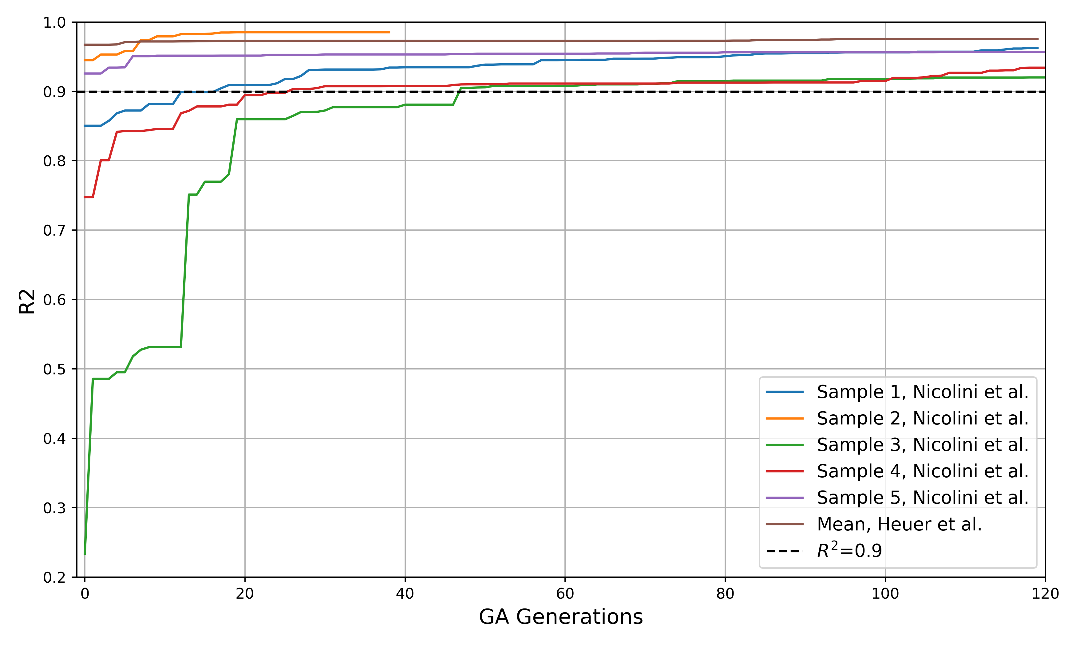
Figure 8: GA evolution of $\overline{\mathcal{R}^{2}}$ values for experimental specimens. 3rd sample by Nicolini et al. [44] requires more than double the amount of generations to converge to a score higher than 0.9.

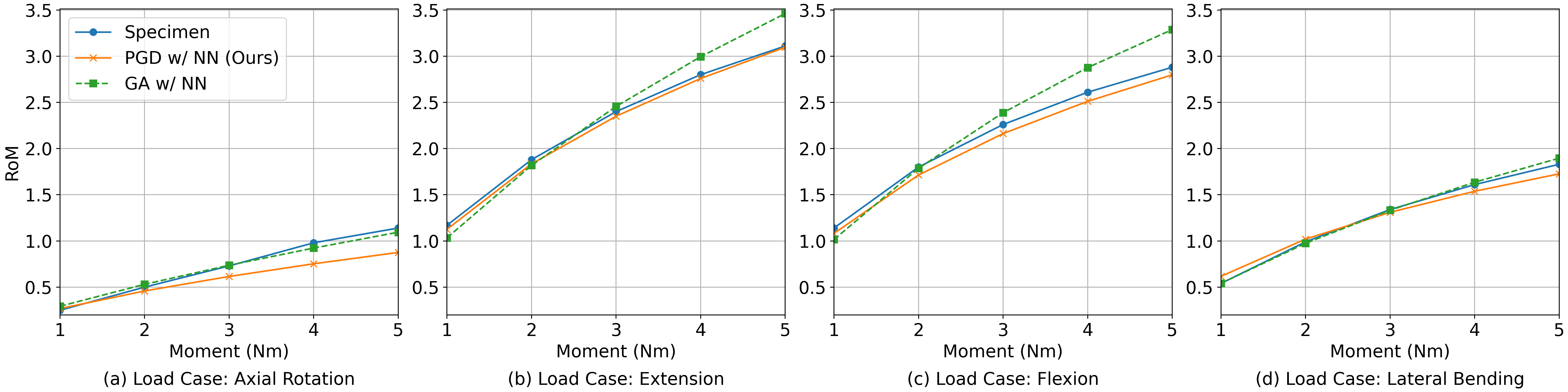
Figure 9: Calibration of Nicolini et al. [44] sample 2

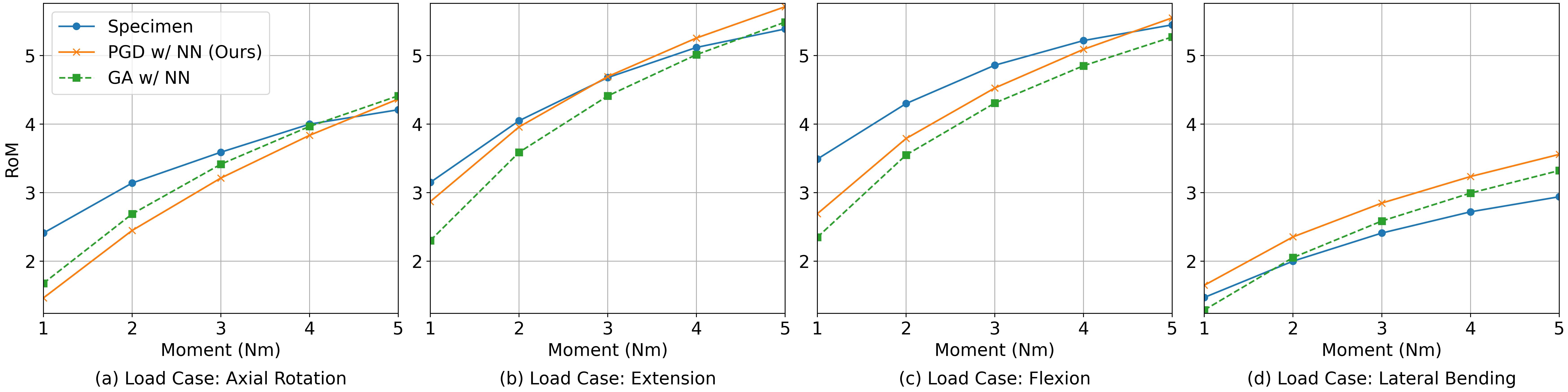
Figure 10: Calibration of Nicolini et al. [44] sample 4

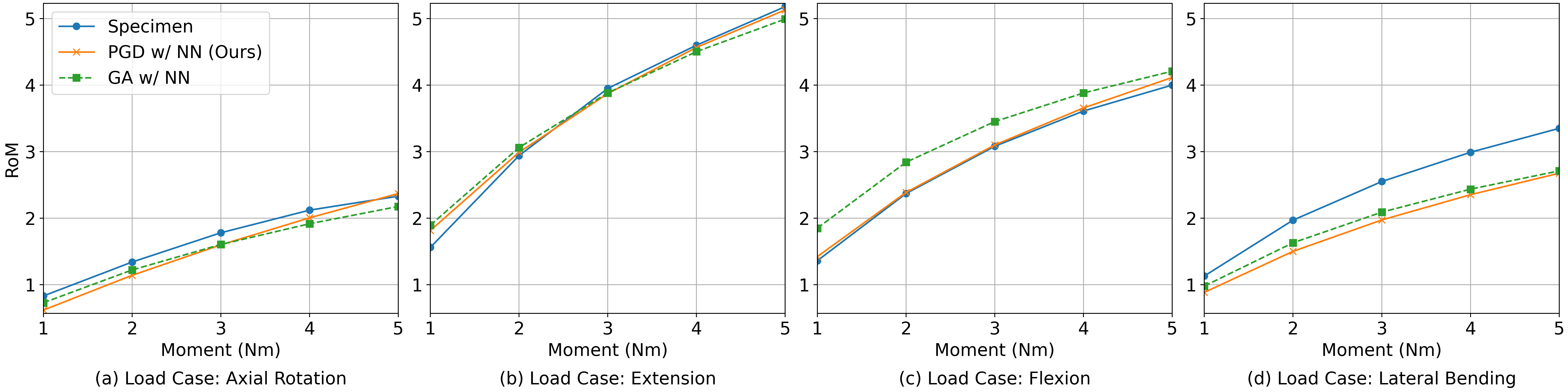
Figure 11: Calibration of Nicolini et al. [44] sample 5

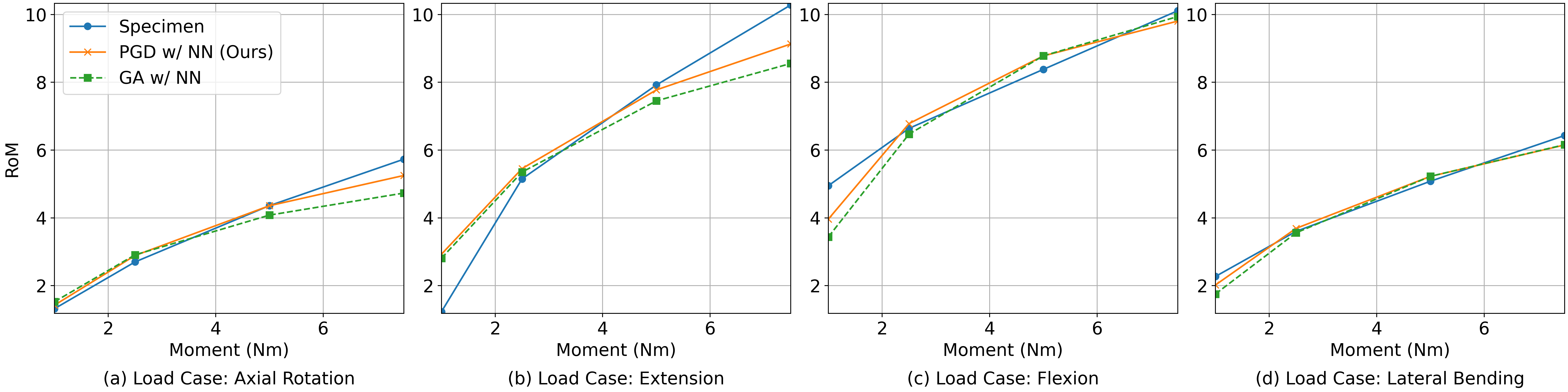
Figure 12: Calibration of Heuer et al. [9] samples mean

Appendix D List of abbreviations

• FE - Finite Element

• GA - Genetic Algorithm

• GP - Gaussian Process

• IVD - Intervertebral Disc

• LHS - Latin hypercube sampling

• LR - Linear Regression

• MAE - Mean Absolute Error

• ML - Machine Learning

• Nm - Newton meter

• NN - Neural Network

• PGD - Projected Gradient Descent

• RF - Random Forest

• RoM - Range-of-Motion

• SVR - Support Vector Machine for Regression

References

- Naoum et al. [2021] S. Naoum, A. V. Vasiliadis, C. Koutserimpas, N. Mylonakis, M. Kotsapas, K. Katakalos, Finite element method for the evaluation of the human spine: a literature overview, Journal of Functional Biomaterials 12 (2021) 43. doi:10.3390/jfb12030043.
- Karajan [2012] N. Karajan, Multiphasic intervertebral disc mechanics: theory and application, Archives of computational methods in engineering 19 (2012) 261–339. doi:10.1007/s11831-012-9073-1.
- Dreischarf et al. [2014] M. Dreischarf, T. Zander, A. Shirazi-Adl, C. Puttlitz, C. Adam, C. Chen, V. Goel, A. Kiapour, Y. Kim, K. Labus, et al., Comparison of eight published static finite element models of the intact lumbar spine: predictive power of models improves when combined together, Journal of biomechanics 47 (2014) 1757–1766. doi:10.1016/j.jbiomech.2014.04.002.
- Damm et al. [2020] N. Damm, R. Rockenfeller, K. Gruber, Lumbar spinal ligament characteristics extracted from stepwise reduction experiments allow for preciser modeling than literature data, Biomechanics and Modeling in Mechanobiology 19 (2020) 893–910. doi:10.1007/s10237-019-01259-6.
- Schmidt et al. [2007] H. Schmidt, F. Heuer, J. Drumm, Z. Klezl, L. Claes, H.-J. Wilke, Application of a calibration method provides more realistic results for a finite element model of a lumbar spinal segment, Clinical biomechanics 22 (2007) 377–384. doi:10.1016/j.clinbiomech.2006.11.008.
- Schlager et al. [2018] B. Schlager, F. Niemeyer, F. Galbusera, D. Volkheimer, R. Jonas, H.-J. Wilke, Uncertainty analysis of material properties and morphology parameters in numerical models regarding the motion of lumbar vertebral segments, Computer methods in biomechanics and biomedical engineering 21 (2018) 673–683. doi:10.1080/10255842.2018.1508571.
- Nicolini et al. [2022] L. F. Nicolini, A. Beckmann, M. Laubach, F. Hildebrand, P. Kobbe, C. R. de Mello Roesler, E. A. Fancello, B. Markert, M. Stoffel, An experimental-numerical method for the calibration of finite element models of the lumbar spine, Medical Engineering & Physics 107 (2022) 103854. doi:10.1016/j.medengphy.2022.103854.
- Schmidt et al. [2006] H. Schmidt, F. Heuer, U. Simon, A. Kettler, A. Rohlmann, L. Claes, H.-J. Wilke, Application of a new calibration method for a three-dimensional finite element model of a human lumbar annulus fibrosus, Clinical biomechanics 21 (2006) 337–344. doi:10.1016/j.clinbiomech.2005.12.001.
- Heuer et al. [2007] F. Heuer, H. Schmidt, Z. Klezl, L. Claes, H.-J. Wilke, Stepwise reduction of functional spinal structures increase range of motion and change lordosis angle, Journal of biomechanics 40 (2007) 271–280. doi:10.1016/j.jbiomech.2006.01.007.
- Zhang et al. [2021] Q. Zhang, T. Chon, Y. Zhang, J. S. Baker, Y. Gu, Finite element analysis of the lumbar spine in adolescent idiopathic scoliosis subjected to different loads, Computers in Biology and Medicine 136 (2021) 104745. doi:10.1016/j.compbiomed.2021.104745.
- Alizadeh et al. [2020] R. Alizadeh, J. K. Allen, F. Mistree, Managing computational complexity using surrogate models: a critical review, Research in Engineering Design 31 (2020) 275–298. doi:10.1007/s00163-020-00336-7.
- Li and Zhang [2023] D. Li, J. Zhang, Finite element model updating through derivative-free optimization algorithm, Mechanical Systems and Signal Processing 185 (2023) 109726. doi:10.1016/j.ymssp.2022.109726.
- Ezquerro et al. [2011] F. Ezquerro, F. G. Vacas, S. Postigo, M. Prado, A. Simón, Calibration of the finite element model of a lumbar functional spinal unit using an optimization technique based on differential evolution, Medical engineering & physics 33 (2011) 89–95. doi:10.1016/j.medengphy.2010.09.010.
- Gruber et al. [2024] G. Gruber, L. F. Nicolini, M. Ribeiro, T. Lerchl, H.-J. Wilke, H. E. Jaramillo, V. Senner, J. S. Kirschke, K. Nispel, Comparative fem study on intervertebral disc modeling: Holzapfel-gasser-ogden vs. structural rebars, Frontiers in Bioengineering and Biotechnology 12 (2024) 1391957. doi:10.3389/fbioe.2024.1391957.
- Kudela and Matousek [2022] J. Kudela, R. Matousek, Recent advances and applications of surrogate models for finite element method computations: a review, Soft Computing 26 (2022) 13709–13733. doi:10.1007/s00500-022-07362-8.
- Phellan et al. [2021] R. Phellan, B. Hachem, J. Clin, J.-M. Mac-Thiong, L. Duong, Real-time biomechanics using the finite element method and machine learning: Review and perspective, Medical Physics 48 (2021) 7–18. doi:10.1002/mp.14602.
- Hammer et al. [2024] M. Hammer, T. Wenzel, G. Santin, L. Meszaros-Beller, J. P. Little, B. Haasdonk, S. Schmitt, A new method to design energy-conserving surrogate models for the coupled, nonlinear responses of intervertebral discs, Biomechanics and Modeling in Mechanobiology (2024) 1–24. doi:10.1007/s10237-023-01804-4.
- Ge et al. [2023] Y. Ge, D. Husmeier, A. Lazarus, A. Rabbani, H. Gao, Bayesian inference of cardiac models emulated with a time series gaussian process, in: Proceedings of the 5th International Conference on Statistics: Theory and Applications (ICSTA’23), 2023, p. 149. doi:10.11159/icsta23.149.
- Cai et al. [2021] L. Cai, L. Ren, Y. Wang, W. Xie, G. Zhu, H. Gao, Surrogate models based on machine learning methods for parameter estimation of left ventricular myocardium, Royal Society open science 8 (2021) 201121. doi:10.1098/rsos.201121.
- Milićević et al. [2022] B. Milićević, M. Ivanović, B. Stojanović, M. Milošević, M. Kojić, N. Filipović, Huxley muscle model surrogates for high-speed multi-scale simulations of cardiac contraction, Computers in Biology and Medicine 149 (2022) 105963. doi:10.1016/j.compbiomed.2022.105963.
- Lostado Lorza et al. [2017] R. Lostado Lorza, F. Somovilla Gomez, R. Fernandez Martinez, R. Escribano Garcia, M. Corral Bobadilla, Improvement in the process of designing a new artificial human intervertebral lumbar disc combining soft computing techniques and the finite element method, in: International Joint Conference SOCO’16-CISIS’16-ICEUTE’16: San Sebastián, Spain, October 19th-21st, 2016 Proceedings 11, Springer, 2017, pp. 223–232. doi:10.1007/978-3-319-47364-2_22.
- Dalton et al. [2023] D. Dalton, D. Husmeier, H. Gao, Physics-informed graph neural network emulation of soft-tissue mechanics, Computer Methods in Applied Mechanics and Engineering 417 (2023) 116351. doi:10.1016/j.cma.2023.116351.
- Hsu et al. [2011] C.-C. Hsu, J. Lin, C.-K. Chao, Comparison of multiple linear regression and artificial neural network in developing the objective functions of the orthopaedic screws, Computer methods and programs in biomedicine 104 (2011) 341–348. doi:10.1016/j.cmpb.2010.11.004.
- Lee et al. [2018] C.-H. Lee, C.-C. Hsu, L. Chaing, An optimization study for the bone-implant interface performance of lumbar vertebral body cages using a neurogenetic algorithm and verification experiment, Journal of Medical and Biological Engineering 38 (2018) 22–32. doi:10.1007/s40846-017-0306-5.
- Sajjadinia et al. [2022] S. S. Sajjadinia, B. Carpentieri, D. Shriram, G. A. Holzapfel, Multi-fidelity surrogate modeling through hybrid machine learning for biomechanical and finite element analysis of soft tissues, Computers in Biology and Medicine 148 (2022) 105699. doi:10.1016/j.compbiomed.2022.105699.
- Moeini et al. [2023] M. Moeini, L. Yue, M. Begon, M. Lévesque, Surrogate optimization of a lattice foot orthotic, Computers in biology and medicine 155 (2023) 106376. doi:10.1016/j.compbiomed.2022.106376.
- da Silva et al. [2021] F. B. da Silva, L. L. Corso, C. A. Costa, Optimization of pedicle screw position using finite element method and neural networks, Journal of the Brazilian Society of Mechanical Sciences and Engineering 43 (2021) 164. doi:10.1007/s40430-021-02880-2.
- Liu et al. [2021] M. Liu, L. Liang, Y. Ismail, H. Dong, X. Lou, G. Iannucci, E. P. Chen, B. G. Leshnower, J. A. Elefteriades, W. Sun, Computation of a probabilistic and anisotropic failure metric on the aortic wall using a machine learning-based surrogate model, Computers in biology and medicine 137 (2021) 104794. doi:10.1016/j.compbiomed.2021.104794.
- Babaei et al. [2022] H. Babaei, E. A. Mendiola, S. Neelakantan, Q. Xiang, A. Vang, R. A. Dixon, D. J. Shah, P. Vanderslice, G. Choudhary, R. Avazmohammadi, A machine learning model to estimate myocardial stiffness from edpvr, Scientific Reports 12 (2022) 5433. doi:10.1038/s41598-022-09128-6.
- Gruber et al. [2024] G. Gruber, M. Atad, M. Ribeiro, L. F. Nicolini, T. Lerchl, J. S. Kirschke, K. Nispel, Comparison of global sensitivity analysis methods for an fe-model of the human intervertebral disc, 2024. Forthcoming.
- Goodfellow et al. [2015] I. J. Goodfellow, J. Shlens, C. Szegedy, Explaining and harnessing adversarial examples, stat 1050 (2015) 20. doi:10.48550/arXiv.1412.6572.
- Mothilal et al. [2020] R. K. Mothilal, A. Sharma, C. Tan, Explaining machine learning classifiers through diverse counterfactual explanations, in: Proceedings of the 2020 conference on fairness, accountability, and transparency, 2020, pp. 607–617. doi:10.1145/3351095.3372850.
- Maso Talou et al. [2021] G. D. Maso Talou, T. P. Babarenda Gamage, M. P. Nash, Efficient ventricular parameter estimation using ai-surrogate models, Frontiers in Physiology 12 (2021) 732351. doi:10.3389/fphys.2021.732351.
- McKay et al. [2000] M. D. McKay, R. J. Beckman, W. J. Conover, A comparison of three methods for selecting values of input variables in the analysis of output from a computer code, Technometrics 42 (2000) 55–61. doi:10.1080/00401706.2000.10485979.
- Holzapfel et al. [2005] G. A. Holzapfel, C. A. Schulze-Bauer, G. Feigl, P. Regitnig, Single lamellar mechanics of the human lumbar anulus fibrosus, Biomechanics and modeling in mechanobiology 3 (2005) 125–140. doi:10.1007/s10237-004-0053-8.
- Yamashita et al. [2023] Y. Yamashita, H. Uematsu, S. Tanoue, Calculation of strain energy density function using ogden model and mooney–rivlin model based on biaxial elongation experiments of silicone rubber, Polymers 15 (2023) 2266. doi:10.3390/polym15102266.
- Brereton and Lloyd [2010] R. G. Brereton, G. R. Lloyd, Support vector machines for classification and regression, Analyst 135 (2010) 230–267. doi:10.1039/B918972F.
- Ke et al. [2017] G. Ke, Q. Meng, T. Finley, T. Wang, W. Chen, W. Ma, Q. Ye, T.-Y. Liu, Lightgbm: A highly efficient gradient boosting decision tree, Advances in neural information processing systems 30 (2017).
- Pedregosa et al. [2011] F. Pedregosa, G. Varoquaux, A. Gramfort, V. Michel, B. Thirion, O. Grisel, M. Blondel, P. Prettenhofer, R. Weiss, V. Dubourg, et al., Scikit-learn: Machine learning in python, the Journal of machine Learning research 12 (2011) 2825–2830.
- Paszke et al. [2019] A. Paszke, S. Gross, F. Massa, A. Lerer, J. Bradbury, G. Chanan, T. Killeen, Z. Lin, N. Gimelshein, L. Antiga, et al., Pytorch: An imperative style, high-performance deep learning library, Advances in neural information processing systems 32 (2019).
- Akiba et al. [2019] T. Akiba, S. Sano, T. Yanase, T. Ohta, M. Koyama, Optuna: A next-generation hyperparameter optimization framework, in: Proceedings of the 25th ACM SIGKDD international conference on knowledge discovery & data mining, 2019, pp. 2623–2631. doi:10.1145/3292500.3330701.
- Srivastava et al. [2014] N. Srivastava, G. Hinton, A. Krizhevsky, I. Sutskever, R. Salakhutdinov, Dropout: a simple way to prevent neural networks from overfitting, The journal of machine learning research 15 (2014) 1929–1958.
- Bubeck et al. [2015] S. Bubeck, et al., Convex optimization: Algorithms and complexity, Foundations and Trends® in Machine Learning 8 (2015) 231–357. doi:10.1561/2200000050.
- Nicolini et al. [2022] L. F. Nicolini, J. Greven, P. Kobbe, F. Hildebrand, M. Stoffel, B. Markert, B. M. Yllera, M. S. Simões, C. R. d. M. Roesler, E. A. Fancello, The effects of tether pretension within vertebral body tethering on the biomechanics of the spine: a finite element analysis, Latin American Journal of Solids and Structures 19 (2022) e442. doi:10.1590/1679-78256932.
- Wirthl et al. [2023] B. Wirthl, S. Brandstaeter, J. Nitzler, B. A. Schrefler, W. A. Wall, Global sensitivity analysis based on gaussian-process metamodelling for complex biomechanical problems, International journal for numerical methods in biomedical engineering 39 (2023) e3675. doi:10.1002/cnm.3675.
- O’Sullivan [1986] F. O’Sullivan, A statistical perspective on ill-posed inverse problems, Statistical science (1986) 502–518. doi:10.1214/ss/1177013525.
- Bajpai and Kumar [2010] P. Bajpai, M. Kumar, Genetic algorithm–an approach to solve global optimization problems, Indian Journal of computer science and engineering 1 (2010) 199–206.
- Echard et al. [2011] B. Echard, N. Gayton, M. Lemaire, Ak-mcs: an active learning reliability method combining kriging and monte carlo simulation, Structural safety 33 (2011) 145–154. doi:10.1016/j.strusafe.2011.01.002.