Pebble-driven migration of low-mass planets
in the 2D regime of pebble accretion

Abstract

Context. Pebbles drifting past a disk-embedded low-mass planet develop asymmetries in their distribution and exert a substantial gravitational torque on the planet, thus modifying its migration rate.

Aims. Our aim is to assess how the distribution of pebbles and the resulting torque change in the presence of pebble accretion, focusing on its 2D regime.

Methods. First, we performed 2D high-resolution multi-fluid simulations with Fargo3D but found that they are impractical for resolving pebble accretion due to the smoothing of the planetary gravitational potential. To remove the smoothing and directly trace pebbles accreted by the planet, we developed a new code, Deneb, which evolves an ensemble of pebbles, represented by Lagrangian superparticles, in a steady-state gaseous background.

Results. For small and moderate Stokes numbers, $\mathrm{St}\lesssim 0.1$, pebble accretion creates two underdense regions with a front-rear asymmetry with respect to the planet. The underdensity trailing the planet is more extended. The resulting excess of pebble mass in front of the planet then makes the pebble torque positive and capable of outperforming the negative gas torque. Pebble accretion thus enables outward migration (previously thought to occur mainly for $\mathrm{St}\gtrsim 0.1$) in a larger portion of the parameter space. It occurs for the planet mass $M_{\mathrm{pl}}\lesssim 3\,M_{\oplus}$ and for all the Stokes numbers considered in our study, $\mathrm{St}\in[10^{-2},0.785]$, assuming a pebble-to-gas mass ratio of $Z=0.01$.

Conclusions. If some of the observed planets underwent outward pebble-driven migration during their accretion, the formation sites of their progenitor embryos could have differed greatly from the usual predictions of planet formation models. To enable an update of the respective models, we provide a scaling law for the pebble torque that can be readily incorporated in N-body simulations.

1 Introduction

The dynamics of planets born within protoplanetary disks are governed by their gravitational interaction with the surrounding disk material. Since gas represents the majority of the disk mass, it is usually considered to be the sole driver of planetary migration (Goldreich & Tremaine, 1979; Kley & Nelson, 2012; Paardekooper et al., 2023), acting by means of the resonant (Goldreich & Tremaine, 1980; Ward, 1986; Korycansky & Pollack, 1993; Ward, 1997), dynamical (Paardekooper, 2014; McNally et al., 2017), magnetohydrodynamic (Baruteau et al., 2011; Uribe et al., 2015; Chametla et al., 2023), or thermal torques (Lega et al., 2014; Benítez-Llambay et al., 2015; Masset, 2017; Chrenko et al., 2017).

Benítez-Llambay & Pessah (2018, hereafter BLP18) only recently demonstrated that small solids (dust, pebbles, or boulders), representing canonically $\sim$$1\%$ of the disk’s mass (cf. Lambrechts & Johansen, 2014), can develop strong azimuthal asymmetries in their surface density owing to their interaction with an embedded low-mass planetary perturber. The angular momentum exchange during this interaction yields an additional torque exerted on the planet, hereinafter referred to as the pebble torque, which is quite often positive, having an opposite sign than the gas torque, which is dominated by the negative Lindblad torque for a broad range of power-law disks (e.g. Tanaka et al., 2002; Coleman & Nelson, 2014).

BLP18 performed 2D multi-fluid hydrodynamic simulations to systematically analyse the dependence of the pebble torque on the planet mass, $M_{\mathrm{pl}}$, and the aerodynamic gas-pebble coupling parametrized by the Stokes number, $\mathrm{St}$ (e.g. Cuzzi et al., 1993). They find that the scattered pebble flow develops a downstream overdense filament in front of the planet and an underdense pebble hole trailing the planet. The excess of pebbles ahead of the planet and their gravitational pull are thus responsible for the pebble torque being positive. The size of the pebble hole is found to increase with increasing $\mathrm{St,}$ and the importance of the pebble torque relative to the gas torque is found to increase with decreasing $M_{\mathrm{pl}}$. BLP18 defined three regimes, namely the gas-dominated regime for which the pebble torque is driven mainly by the filament ($\mathrm{St}\lesssim 0.25$), the gravity-dominated regime for which the contribution of the hole is significant ($\mathrm{St}\gtrsim 0.35$), and a transitional regime ($\mathrm{St}\simeq 0.25$–$0.35$) in which an increased concentration of pebbles accumulates at the edge of the hole and can actually result in a negative pebble torque (due to a mass excess trailing the planet). Assuming a pebble-to-gas mass ratio of $Z=0.01$ and taking an Earth-mass planet as an example, the pebble torque would overcome the gas torque and revert migration from inwards to outwards for $\mathrm{St}\gtrsim 0.1$, with the exception of the transitional regime ($\mathrm{St}\simeq 0.25$; see also Guilera et al., 2023).

When embedded in a sea of pebbles, the planet is also expected to undergo pebble accretion (Ormel & Klahr, 2010; Lambrechts & Johansen, 2012). Pebbles become captured by the planet even from large impact parameters (comparable to the planet’s Hill radius in the most favourable cases) because the accretion cross-section is enhanced by the gas drag. As a pebble becomes deflected by the planet, its kinetic energy is dissipated by the aerodynamic friction and the pebble can settle onto the planetary surface (Johansen & Lambrechts, 2017; Ormel, 2017). Since pebble accretion should occur automatically for a planet embedded in a gas-pebble disk, it is definitely worthwhile to examine its influence on the pebble distribution generating the pebble torque.

In BLP18, the process of pebble accretion was neglected. The authors argued that the dynamics of pebbles entering the Hill sphere might not be captured accurately by their model, and they ignored the disk material located in the inner half of the Hill sphere in their torque calculations. The first attempt to include pebble accretion in the context of pebble-driven torque was done by Regály (2020). In their multi-fluid model, however, pebble accretion was achieved via an ad hoc reduction of the pebble surface density, with the accretion radius fixed and the accretion efficiency a free parameter. In other words, pebble accretion was not achieved self-consistently by converging pebble trajectories (or streamlines in their case) at the planet location. One of the difficulties in studying pebble accretion using global 2D multi-fluid models arises due to the smoothing of the planetary gravitational potential, as we show in our manuscript (see also Regály, 2020).

In our study, we focused on the 2D limit of pebble accretion in which pebbles are accreted from a layer that is thinner than the vertical extent of the planet’s feeding radius (Lambrechts & Johansen, 2012). We mainly relied on a hybrid fluid-particle method in which pebbles are modelled as Lagrangian superparticles. This approach allowed us to remove the smoothing of the planetary potential for pebbles and track their trajectories very close to the planetary surface, resolving pebble accretion in a self-consistent manner. Additionally, the Lagrangian approach captures the effect of mutually crossing pebble trajectories, which is not possible in the fluid approximation. By analysing the pebble torque resulting from our superparticle model, we show that pebble accretion can expand the parameter range in which the pebble torque is positive and supersedes the gas torque.

2 Methods

The configuration that we studied corresponds to a planet with the mass $M_{\mathrm{pl}}$ on a circular orbit at a distance $r_{\mathrm{pl}}=5.2\,\mathrm{au}$ from the central star. The planet is embedded in a 2D disk of gas and pebbles, which it perturbs via its gravitational potential. In this study, the planetary orbit is not evolving, we only measured the gravitational torque exerted by the perturbed gas and pebble distributions on the planet. The reference frame is heliocentric and corotating with the planet.

2.1 Pebbles as a fluid

To establish a firm link to previous works, we performed multi-fluid simulations in which pebbles are treated as a pressureless fluid feeling the aerodynamic friction due to its relative motion with respect to the gas fluid (we neglected the back-reaction of dust on gas). We used the publicly available code Fargo3D, which contains the same model ingredients that were used in BLP18 and we considered a polar mesh with coordinates $(r,\varphi)$.

The gas fluid is treated as a locally isothermal disk with a constant aspect ratio $h(r)=0.05$. The initial surface density profile follows

$$\Sigma_{\mathrm{g}}(r)=(50\,\mathrm{g}\,\mathrm{cm}^{-2})\left(\frac{r}{r_{\mathrm{pl}}}\right)^{-1/2}\,,$$ (1)

the radial gas velocity is initially zero, $v_{r}=0$, and the rotational gas velocity is

$$v_{\varphi}(r)=\Omega_{\mathrm{K}}r\sqrt{1-\frac{3}{2}h^{2}}=v_{\mathrm{K}}(1-\eta)\,,$$ (2)

where $\Omega_{\mathrm{K}}$ is the Keplerian frequency, $v_{\mathrm{K}}=r\Omega_{\mathrm{K}}$ is the Keplerian orbital velocity, and $\eta$ is the pressure support parameter defined as

$$\eta=-\frac{1}{2}h^{2}\frac{\partial\log P}{\partial\log r}\,,$$ (3)

with $P=(hv_{\mathrm{K}})^{2}\Sigma_{\mathrm{g}}$ being the pressure.

The pebble fluid is then initialized via the pebble-to-gas ratio $Z=0.01$ as

$$\Sigma_{\mathrm{p}}=Z\Sigma_{\mathrm{g}}\,,$$ (4)

and the initial velocities follow the expressions (see Adachi et al., 1976; Guillot et al., 2014; Chrenko et al., 2017)

$$u_{\varphi}=v_{\mathrm{K}}-\frac{1}{1+\mathrm{St}^{2}}\left(\eta v_{\mathrm{K}}+\frac{\mathrm{St}}{2}v_{r}\right)\,,$$ (5)

$$u_{r}=-\frac{2\mathrm{St}}{1+\mathrm{St}^{2}}\left(\eta v_{\mathrm{K}}-\frac{1}{2\mathrm{St}}v_{r}\right)\,.$$ (6)

The Stokes number $\mathrm{St}$ is considered a free parameter and expresses the strength of the aerodynamic drag felt by pebbles:

$$\@vec{a}_{\mathrm{drag}}=\frac{\@vec{v}-\@vec{u}}{t_{\mathrm{s}}}=\frac{\Omega_{\mathrm{K}}}{\mathrm{St}}\left(\@vec{v}-\@vec{u}\right)\,,$$ (7)

where $t_{\mathrm{s}}$ is the stopping time. For the considerations of our study, it is important to point out that when the initial conditions of gas and pebbles are combined together, the radial mass flux of pebbles facilitated by the drag is uniform. This fact is demonstrated in Appendix A and ensures that the mass flux in pebbles drifting past the planet does not fluctuate in time.

Compared to BLP18, our multi-fluid simulations differ in the following aspects. The radial grid span is narrower, covering $0.7$–$1.3\,r_{\mathrm{pl}}$. The grid spacing is uniform in all directions, with the resolution of $N_{r}=2400$ radial rings and $N_{\varphi}=24576$ azimuthal sectors. The motivation for this relatively large resolution is to maintain the radial spacing equal to the finest level of the non-uniform grid of BLP18 while doubling the resolution in azimuth to keep the grid cells square-shaped at the planet location, having the size of $2.5\times 10^{-4}\,r_{\mathrm{pl}}$. The Shakura-Sunyaev viscosity parameter (Shakura & Sunyaev, 1973) assumed for the gas fluid is $\alpha=10^{-4}$ (compared to $\alpha=3\times 10^{-3}$ used in BLP18, ).

As for the boundary conditions for gas and pebble fluids, we used a linear extrapolation for the surface densities, a Keplerian extrapolation for azimuthal velocities, and reflective boundary conditions for radial velocities. Furthermore, wave-killing zones (de Val-Borro et al., 2006) in which hydrodynamic quantities are damped towards the initial state were applied at $r<0.77\,r_{\mathrm{pl}}$ and $r>1.18\,r_{\mathrm{pl}}$. We point out that we ignored the indirect acceleration term related to the reflex motion of the star induced by the disk itself (Crida et al., 2022).

In 2D hydrodynamic simulations of planet-disk interactions, it is customary to consider a smoothed Plummer-type gravitational potential for the planet:

$$\Phi_{\mathrm{pl}}=-\frac{GM_{\mathrm{pl}}}{\sqrt{d^{2}+\epsilon^{2}}}\,,$$ (8)

where $d$ is the distance from the planet to a point of interest and $\epsilon$ is the smoothing length. The purpose of $\epsilon$ is twofold. First, it is needed to avoid numerical divergence of the potential term for grid cells overlapping with the planet location. Second, $\epsilon$ can be fine-tuned to account for the fact that in reality the planet is not interacting with a 2D distribution of matter; it is instead interacting with a 3D disk of non-zero thickness. For isothermal gas disks, it is possible to make an educated guess of $\epsilon$ so that the gas torque acting on the planet in the 2D model is similar to the result of 3D simulations (Müller et al., 2012). Typically, $\epsilon=0.4$–$0.7H_{\mathrm{g}}$, where $H_{\mathrm{g}}=hr$ is the pressure scale height.

However, the choice of $\epsilon$ for pebbles is less clear. A comprehensive comparison of 2D and 3D pebble-driven torque has never been performed; intuitively, 3D pebble-driven torque will necessarily depend on the level of turbulent stirring (e.g. Dubrulle et al., 1995). In the two most extreme cases, large pebbles in a laminar disk would settle all the way to the midplane, whereas small pebbles in a turbulent disk might be completely mixed with the gas, having the same scale height.

For the purpose of our study, it is important to keep backward comparability; we thus followed BLP18 and set $\epsilon=1\,R_{\mathrm{H}}$ for both gas and pebbles when running multi-fluid simulations. However, as we show later, this prevents the model from capturing pebble accretion, and therefore, we also employed methods that enabled us to relax the value of $\epsilon$ for pebbles.

2.2 Pebbles as superparticles

To recover pebble accretion, we examined the limiting case in which all pebbles are settled in a thin layer close to the midplane of the protoplanetary disk. In that case, they are being accreted in the 2D regime (e.g. Lambrechts & Johansen, 2012; Morbidelli & Nesvorný, 2012; Morbidelli et al., 2015) and from a physical point of view, there is no argument for such a pebble disk to evolve in a smoothed planetary potential; instead one should set $\epsilon=0$. The dynamics of pebbles within an unsmoothed planetary potential might become very complex, including crossing and repeatedly scattered trajectories (see e.g. Johansen & Lambrechts, 2017) that the grid-based fluid approximation fails to capture (it mainly captures a local mean state of multiple pebbles). Furthermore, it is not clear if the fluid approximation for pebbles can safely be used with $\epsilon$ smaller than the minimum size of the grid cells.

For these reasons, we decided to track individual pebble trajectories using a Lagrangian approach. We developed a new code that reads the gas distribution and velocities resulting from multi-fluid runs with Fargo3D and evolves an ensemble of superparticles within this distribution. Since we assumed that the planetary orbit is not evolving and the frame corotates with the planet, the gas fields obtained by Fargo3D represent a steady state and are suitable for an ex-post analysis of the pebble evolution.

For future reference, our new hybrid fluid-particle code is named Deneb (an abbreviation for ‘dust evolution near embedded bodies’). The trajectories of superparticles are integrated based on their equation of motion in the heliocentric frame (e.g. Liu & Ormel, 2018):

$$\frac{\mathrm{d}^{2}\@vec{r}}{\mathrm{d}t^{2}}=-GM_{\star}\frac{\@vec{r}}{r^{3}}+GM_{\mathrm{pl}}\left(\frac{\@vec{r}_{\mathrm{pl}}-\@vec{r}}{|\@vec{r}_{\mathrm{pl}}-\@vec{r}|^{3}}-\frac{\@vec{r}_{\mathrm{pl}}}{r_{\mathrm{pl}}^{3}}\right)+\@vec{a}_{\mathrm{drag}}\,,$$ (9)

where $M_{\star}$ is the stellar mass. Of course, the denominator of the planet-superparticle acceleration can be again smoothed using $\epsilon$, if needed. We use the smoothing in superparticle simulations only to enable a comparison with multi-fluid simulations.

Since the underlying gas disk is described on a 2D polar grid, it is convenient to solve Eq. (9) in polar coordinates ($r$, $\varphi$) and for dynamical variables ($u_{r}$, $l$), where $l=ru_{\varphi}$ is the specific angular momentum of a superparticle. The trajectories are propagated using the second-order drift-kick-drift scheme of Mignone et al. (2019) based on the exponential midpoint method. The whole N-body system is rotated after each drift to keep the planet at $\varphi_{\mathrm{pl}}=0$ and to synchronize superparticles with the underlying gas disk. Gas quantities are inferred at locations of superparticles using the bilinear interpolation. To convert the number density of superparticles to the pebble surface density $\Sigma_{\mathrm{p}}$ and map it back to the polar grid, the cloud-in-cell method is used.

Unless specified otherwise, we initialize $N_{\mathrm{sp}}=5\times 10^{6}$ superparticles between $r_{\mathrm{min}}=0.8$ and $r_{\mathrm{max}}=1.2\,r_{\mathrm{pl}}$. The initial $r(t=0)$ of superparticles is selected randomly uniformly between $0$ and $1$ from the following probability distribution (e.g. Baruteau et al., 2019):

$$P(r)=\frac{\int_{r_{\mathrm{min}}}^{r}\Sigma_{\mathrm{p}}(r)\mathrm{d}r}{\int_{r_{\mathrm{min}}}^{r_{\mathrm{max}}}\Sigma_{\mathrm{p}}(r)\mathrm{d}r}\,.$$ (10)

The azimuth $\varphi(t=0)$ is sorted out randomly uniformly between $-\pi$ and $\pi$. Each superparticle is assigned the same mass $m_{\mathrm{sp}}$ so that the total mass in pebbles $M_{\mathrm{p}}=N_{\mathrm{sp}}m_{\mathrm{sp}}$ is equal to $ZM_{\mathrm{g}}$, where $M_{\mathrm{g}}$ is the total gas mass between $r_{\mathrm{min}}$ and $r_{\mathrm{max}}$. We point out, however, that the superparticles behave as massless test particles throughout the simulation; the purpose of $m_{\mathrm{sp}}$ is only to reconstruct $\Sigma_{\mathrm{p}}$ and the torque that it exerts on the planet. The initial velocities of each superparticle are again chosen according to Eqs. (5) and (6).

Pebble accretion is achieved in two steps. The first step, as already mentioned, is to set $\epsilon=0$, which ensures an occurrence of trajectories that converge and accumulate pebbles at the planet location (see Sect. 3.3). The second step is to discard these captured superparticles from the simulation, and we did so when $d\equiv|\@vec{r}_{\mathrm{pl}}-\@vec{r}|<3R_{\mathrm{surf}}$, where $R_{\mathrm{surf}}$ is the planetary surface radius (obtained from $M_{\mathrm{pl}}$ for the material density $\rho_{\mathrm{pl}}=1.5\,\mathrm{g}\,\mathrm{cm}^{-3}$). The choice of the accretion distance $3R_{\mathrm{surf}}$ is based on the fact that we do not properly resolve the formation of the first planetary atmospheres (Ormel et al., 2015a; Béthune & Rafikov, 2019), which could influence the final stage of settling of pebbles onto the planet (D’Angelo & Bodenheimer, 2024). However, it is usually safe to assume that pebbles that manage to enter the Bondi radius eventually become accreted (e.g. Popovas et al., 2018).

Drifting superparticles are also discarded from the simulation whenever they cross $r_{\mathrm{min}}$. To preserve the radial mass flux of pebbles towards the planet, new superparticles are introduced in the simulation at $r_{\mathrm{max}}$ to maintain the total number of superparticles in the annulus $r\in[0.92,1]\,r_{\mathrm{max}}$ constant. In our first numerical tests, we found that because the superparticles are revived at a fixed radial distance, artificial disturbances of $\Sigma_{\mathrm{p}}$ are often produced at the outer boundary because its geometry does not reflect the local shape of trajectories — they often exhibit a kink either if $\mathrm{St}$ is low and particles cross the outer gaseous spiral arm or if $\mathrm{St}$ is large and particles perform a small epicyclic oscillation after passing through the opposition with the planet. These effects are summarized in Appendix B. The boundary artefacts are undesired because they can spread inwards owing to the drag-induced drift. To disperse the artefacts, we assigned random noise to the background gas velocities with an amplitude that is equal to $5\%$ of the respective velocity component at $r_{\mathrm{max}}$ and decreases linearly to zero as $r$ decreases over the interval $r\in[0.92,1]\,r_{\mathrm{max}}$.

The integration time step in our code depends on the distance from the planet. When $d>1.75R_{\mathrm{H}}$, we set $\mathrm{d}t=2\times 10^{-3}P_{\mathrm{orb}}$, where $P_{\mathrm{orb}}$ is the orbital timescale of the planet. When $d\in(0.2,1.75]R_{\mathrm{H}}$, the time step is $\mathrm{d}t=2\times 10^{-4}P_{\mathrm{orb}}$. Finally, we set $t=5\times 10^{-6}P_{\mathrm{orb}}$ when $d\leq 0.2R_{\mathrm{H}}$. The choice of the time step is empirical: we reduced the time step at the above-defined ranges of $d$ until the resulting changes of superparticle trajectories became negligible. We show in Appendix C that our time step choice leads to pebble accretion rates matching those from literature. The Deneb code is further tested against an independent fluid-particle code Dusty FARGO-ADSG (Baruteau & Zhu, 2016) in Appendix D.

Set	Code	$\epsilon/R_{\mathrm{H}}$	$R_{\mathrm{c}}/R_{\mathrm{H}}$	Pebble removal
MfaE1	Fargo3D	$1$	$0.5$	N/A
MspE1	Deneb	$1$	$0.5$	N/A
MspE0	Deneb	$0$	$0.1$	$d<3\,R_{\mathrm{surf}}$
Parameter	List of values
$M_{\mathrm{pl}}/M_{\oplus}$	$0.33$, $0.49$, $0.71$, $1.04$, $1.51$, $2.21$, $3.22$, $4.7$
$\mathrm{St}$	$0.01$, $0.014$, $0.021$, $0.03$, $0.043$, $0.062$, $0.089$, $0.127$, $0.183$, $0.264$, $0.379$, $0.546$, $0.785$

Table 1: Overview of simulation sets (top part of the table) and main simulation parameters (bottom part of the table).

2.3 Model overview and diagnostics

Our main parameters are the planet mass $M_{\mathrm{pl}}$, the Stokes number of pebbles $\mathrm{St}$, and the smoothing length of the planetary potential $\epsilon$ felt by pebbles. We logarithmically sampled eight and thirteen values from intervals $M_{\mathrm{pl}}\in[0.33,4.7]\,M_{\oplus}$ and $\mathrm{St}\in[0.01,0.785]$, respectively, thus ensuring an overlap with the slightly more extended parameter space of BLP18 (see Table 1).

To distinguish between different sets of simulations, we use abbreviations based on the following conventions: Mfa stands for ‘models using the fluid approximation’ (i.e. Fargo3D simulations), Msp stands for ‘models using superparticles’ (i.e. Deneb simulations), and E1 or E0 indicate whether the potential smoothing length for pebbles is $\epsilon=1$ or $0\,R_{\mathrm{H}}$. Our main sets of models are then designated MfaE1, MspE1, and MspE0 (see Table 1). When referring to a specific simulation from a given set, we write, for instance, MfaE1_M0.3St0.014, where the suffix gives the respective values of the planet mass (in Earth masses, $M_{\oplus}$) and the Stokes number.

As Fargo3D calculations are computationally intensive due to the large domain resolution, and also in order to maintain backward consistency with BLP18, the simulations MfaE1 span 50 orbital periods of the planet. On the other hand, our superparticle simulations MspE1 and MspE0 are extended over 200 orbital periods to ensure that the measured pebble torque is converged (see Sect. 3.1).

The torque acting on the planet is evaluated as

$$\Gamma=\int\limits_{\mathrm{disk}}\Sigma_{i}\left(\@vec{r}_{\mathrm{pl}}\times\@vec{a}_{\mathrm{g}}\right)\mathrm{d}S\,,$$ (11)

where $\Sigma_{i}$ is the torque-generating mass distribution ($\Sigma_{\mathrm{g}}$ for the gas torque or $\Sigma_{\mathrm{p}}$ for the pebble torque), $\@vec{a}_{\mathrm{g}}$ is the specific gravitational acceleration arising from a disk element, and the integral reduces to a discrete sum over the simulated disk patch. For simulation sets MfaE1 and MspE1, we followed BLP18 and excluded a part of the material located within the Hill sphere from the torque evaluation. In each grid cell, we multiplied the material mass prior to the torque computation using the exclusion function

$$f_{\mathrm{cut}}=\cases{1}&d>R_{\mathrm{c}}+0.5R_{\mathrm{H}}\,,\\ \sin^{2}{\left[\pi\left(\frac{d-R_{\mathrm{c}}}{R_{\mathrm{H}}}\right)\right]}d\in[R_{\mathrm{c}},R_{\mathrm{c}}+0.5R_{\mathrm{H}}]\,,\\ 0d<R_{\mathrm{c}}\,,{}$$ (12)

where $R_{\mathrm{c}}=0.5\,R_{\mathrm{H}}$ is the cutoff radius. As for our simulation set MspE0, our nominal choice is $R_{\mathrm{c}}=0.1\,R_{\mathrm{H}}$, which helps reduce torque oscillations due to the stochasticity in the delivery of superparticles towards the accretion radius. However, the choice of $R_{\mathrm{c}}$ is rather arbitrary and we thus explore its influence on the torque value in Sect. 3.4.

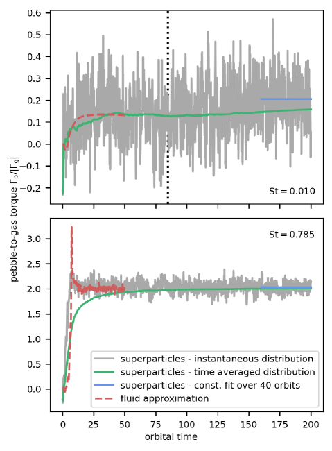
Figure 1: Time evolution of the pebble-to-gas torque ratio, $\Gamma_{\mathrm{p}}/|\Gamma_{\mathrm{g}}|$, as a comparison of the fluid and superparticle approximations for the planet mass $M_{\mathrm{pl}}=1.51\,M_{\oplus}$. The Stokes numbers are $\mathrm{St}=0.01$ (top) and $0.785$ (bottom). The planet potential felt by pebbles is smoothed using $\epsilon=1\,R_{\mathrm{H}}$. The dashed red curve corresponds to simulations obtained with the Fargo3D code (set MfaE1). For simulations obtained with the Deneb code (set MspE1,) we distinguish: the torque arising from the instantaneous distribution of superparticles (grey curve), the torque corresponding to the time-averaged superparticle distribution (green curve), and a constant fit of the instantaneous torque (blue line). The dotted vertical line is the approximate time it takes pebbles to radially drift across the horseshoe region of the planet.

3 Results

3.1 First look at the torque measurements

We first explored a typical measurement of the pebble torque with Fargo3D and Deneb, focusing on simulation sets MfaE1 and MspE1. Figure 1 shows the ratio between the pebble torque $\Gamma_{\mathrm{p}}$ and the absolute value of the gas torque $|\Gamma_{\mathrm{g}}|$. The later is always taken from fluid simulations with Fargo3D as we assume a non-evolving gas distribution in our superparticle simulations.

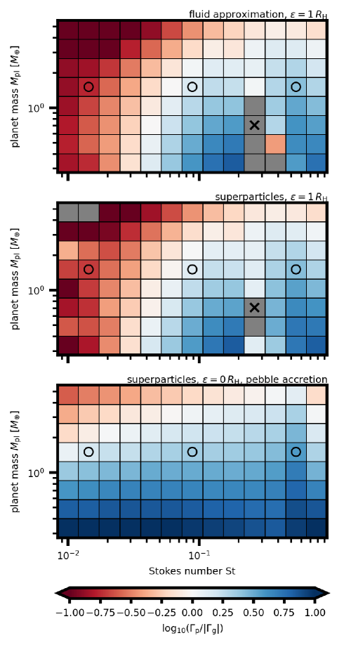
Figure 2: Torque map in the spirit of BLP18 showing the logarithm of the pebble-driven torque, $\Gamma_{\mathrm{p}}$, scaled by the magnitude of the gas-driven torque, $|\Gamma_{\mathrm{g}}|$. Grey patches correspond to parameter combinations for which $\Gamma_{\mathrm{p}}<0$. Circles mark the simulations that are discussed in detail in Figs. 3 and 4, while crosses mark the simulation analysed in Figs. 12 and 13. Top: Multi-fluid simulations with Fargo3D (set MfaE1) using the planetary potential smoothing length $\epsilon=1\,R_{\mathrm{H}}$ for both gas and pebbles, and the material exclusion radius for the torque calculation $R_{\mathrm{c}}=0.5\,R_{\mathrm{H}}$. Middle: Simulations with Lagrangian superparticles representing pebbles (set MspE1). Parameters are the same as in the top panel, except for the time span of 200 orbital periods. Bottom: Simulations with Lagrangian superparticles avoiding the potential smoothing for pebbles (set MspE0), $R_{\mathrm{c}}=0.1\,R_{\mathrm{H}}$, and allowing for pebble accretion.

When measuring $\Gamma_{\mathrm{p}}$ with the Deneb code, we tested two approaches. The first approach is to record the torque arising from the $\Sigma_{\mathrm{p}}(r,\varphi)$ distribution related to the instantaneous positions of superparticles at the given time $t$. Since the number of superparticles within each cell of the 2D mesh fluctuates in time, so does the instantaneous torque value (grey curve in Fig. 1). The pebble torque is then obtained by fitting a constant over a sufficiently long period of time (blue line in Fig. 1) defined in our case as the last forty orbital periods of the planet. The second approach is to record a time-averaged superparticle (and density) distribution in each cell of the grid and calculate the pebble torque from it (green curve in Fig. 1). For the purpose of the time averaging, the superparticle distribution is recorded 50 times per planetary orbit.

In the limit of large Stokes numbers (bottom panel of Fig. 1; $\mathrm{St}=0.785$), all torque measurements converge at similar values and we see that there is a very good agreement between the superparticle and fluid approximations. However, the situation in the limit of small Stokes numbers (top panel of Fig. 1; $\mathrm{St}=0.01$) is different. We see that while the torque measurements overlap at first and there seems to be a mock convergence, the torque value can undergo additional variations after a timescale roughly equal to the crossing time of the horseshoe region due to the radial drift of pebbles. Using the horseshoe half-width $x_{\mathrm{s}}=1.05r_{\mathrm{pl}}\sqrt{M_{\mathrm{pl}}/(hM_{\star})}$ (Jiménez & Masset, 2017) and $u_{r}\simeq-2\mathrm{St}\eta v_{\mathrm{K}}$ (Eq. 6), we get $t_{\mathrm{cross}}=2x_{\mathrm{s}}/|u_{r}|\simeq 85P_{\mathrm{orb}}$ for the top panel of Fig. 1, as indicated by the vertical dotted line. In this particular case, one can see that the torque obtained in our superparticle simulation starts to slowly increase at $t>t_{\mathrm{cross}}$ and departs from the Fargo3D result. At the end of the simulation, there is also a mismatch between $\Gamma_{\mathrm{p}}$ calculated using the constant fit (blue line) and using the time-averaged superparticle distribution (green curve). The reason for the difference is that the time-averaged distribution is plagued by the recordings done at $t<t_{\mathrm{cross}}$ and thus it takes a relatively large amount of time for it to react to changes of the instantaneous superparticle distribution. In the following, all our measurements of $\Gamma_{\mathrm{p}}$ in simulation sets MspE1 and MspE0 will be obtained by fitting a constant to the instantaneous torque curve.

3.2 Parametric study of the pebble torque

Figure 2 summarizes the pebble torque relative to the gas torque across the entire parameter space. Since the same kind of a torque map (showing $\log_{10}(\Gamma_{\mathrm{p}}/|\Gamma_{\mathrm{g}}|)$) was used in BLP18, one can directly compare a subset of their figure 2 with the top panel of our Fig. 2, corresponding to the simulations MfaE1. Unsurprisingly, the comparison yields an excellent agreement. Minor differences can be found that can be attributed either to the improved resolution that we used or to the lower disk viscosity that we assumed.

Next, Figure 2 enables to compare the simulation sets MfaE1 (top) and MspE1 (middle). Clearly, there is an overall agreement between the two, which confirms the robustness of the superparticle method for measuring $\Gamma_{\mathrm{p}}$. There are, however, two distinct regions of the parameter space that exhibit differences. The first region is located at $\mathrm{St}\lesssim 0.015$. Within this region, the differences arise as explained in Sect. 3.1: the drift of pebbles is relatively slow compared to the timescale of the MfaE1 simulations ($50$ orbital periods) and thus the angular momentum exchange between the planet and pebbles near the horseshoe region is not necessarily in a steady state. The second region is located roughly at $\mathrm{St}\in[0.26,0.38]$ and $M_{\mathrm{pl}}\lesssim 1.5\,M_{\oplus}$. It corresponds to the transitional regime defined by BLP18 (see also Sect. 1) and in several cases, it exhibits negative pebble torques (therefore undefined in the logarithmic scale of Fig. 2). The reason why the superparticle approach predicts different $\Gamma_{\mathrm{p}}$ is that it resolves fine substructures in the pebble flow with better accuracy (see Appendix E).

Finally, and most importantly, the bottom panel of Fig. 2 provides the predicted pebble torque for the simulation set MspE0, that is, when the planetary potential for pebbles is no longer smoothed and pebble accretion is accounted for. Substantial changes occur in the map and we summarize them as follows:

• The whole parameter space is now regular and $\Gamma_{\mathrm{p}}>0$ for every explored combination of $M_{\mathrm{pl}}$ and $\mathrm{St}$.

• For a fixed planet mass, the dependence of $\Gamma_{\mathrm{p}}$ on $\mathrm{St}$ shows weaker variations than with $\epsilon=1\,R_{\mathrm{H}}$.

• The pebble torque at $\mathrm{St}\lesssim 0.1$ becomes much stronger, exceeding the gas torque by a factor of several for Earth-sized planets and by a factor of $10^{1}$ for sub-Earths. The scaling with the planet mass is the same as at $\mathrm{St}\gtrsim 0.1$—the lower is the planet mass, the stronger $\Gamma_{\mathrm{p}}$ becomes relative to the gas-driven torque.

• At $\mathrm{St}\gtrsim 0.1$ (aside from the irregular region found in top and middle panels of Fig. 2), the overall character of the map remains the same as in simulation sets MfaE1 and MspE1, only the pebble torque magnitude seems to be systematically shifted to larger values.

• All these facts suggest that the influence of pebble accretion in the 2D regime has the largest impact on the pebble torque for low Stokes numbers (see Sect. 3.4 for a confirmation). This influence is important as it significantly extends the portion of the parameter space in which planet migration can become dominated by the pebble torque in protoplanetary disks.

3.3 Influence of pebble accretion on the torque-generating surface density

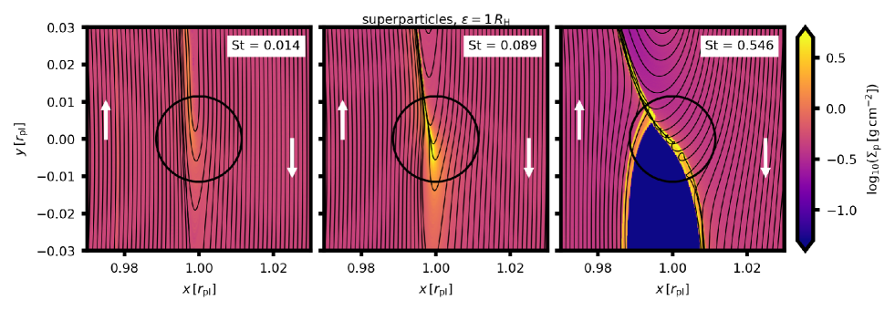
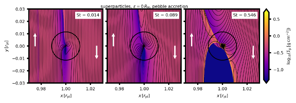
Figure 3: Surface density of pebbles, $\Sigma_{\mathrm{p}}$, near a $1.51\,M_{\oplus}$ planet for three values of the Stokes number: $\mathrm{St}=0.014$, $0.089$, and $0.546$ (left, middle, and right columns, respectively). The black circle shows the extent of the Hill radius, and the white arrows show the direction of the shear motion relative to the planet. In an inertial frame, the planet would orbit in the $y>0$ direction. Radial drift of pebbles occurs in the $x<0$ direction. The lower and upper limits of the logarithmic colour palette correspond to the initial pebble surface density at the planet location multiplied by $10^{-1}$ and $10^{1}$, respectively. Top: $\Sigma_{\mathrm{p}}$ results directly from Fargo3D multi-fluid simulations. The black curves are streamlines of the pebble fluid. The planetary potential smoothing for pebbles is $\epsilon_{\mathrm{p}}=1\,R_{\mathrm{H}}$, and the simulation time is $t=50\,P_{\mathrm{orb}}$. Middle: $\Sigma_{\mathrm{p}}$ calculated from the distribution of superparticles by the cloud-in-cell method and averaged in time. The black curves are trajectories of individual superparticles. The potential smoothing for pebbles is $\epsilon_{\mathrm{p}}=1\,R_{\mathrm{H}}$, and the simulation time is $t=200\,P_{\mathrm{orb}}$ Bottom: As in the middle row but avoiding potential smoothing for pebbles and allowing for pebble accretion.

Generally speaking, the pebble torque exists due to a front-rear asymmetry in the pebble surface density $\Sigma_{\mathrm{p}}$ with respect to the planet. Therefore, in order to understand what drives the changes of $\Gamma_{\mathrm{p}}$ in Fig. 2, it is necessary to examine where the asymmetry is generated and how it relates to the orbital dynamics of pebbles. With this in mind, we display $\Sigma_{\mathrm{p}}$ in a close proximity of a $M_{\mathrm{pl}}=1.51\,M_{\oplus}$ planet in Fig. 3. The rows of Fig. 3 correspond to simulation sets MfaE1, MspE1, and MspE0, respectively, while the columns correspond to $\mathrm{St}=0.014$, $0.089$, and $0.546$, respectively.

The dynamics of pebbles in the first row of Fig. 3 (simulations MfaE1) matches the findings of BLP18. When the Stokes number is small and aerodynamic coupling with the gas is substantial, one can see that a small part of the pebble streamlines is concentrated downstream in front of the planet. This leads to a formation of an overdense filament responsible for a positive, albeit small, torque. As the Stokes number starts to increase, the filament becomes more prominent and starts to extend also into the region trailing the planet. Pebble streamlines suffer a noticeable deflection when crossing the Hill sphere. Finally, in the limit of large Stokes numbers, the torque is dominated by a formation of a large-scale underdense hole in the pebble distribution trailing the planet. The filament is present not only in front of the planet, but also behind the planet, encircling the pebble hole. Clearly, the hole is formed because streamlines preferentially encircle this region, isolating it from the incoming flux of pebbles. The streamlines encircling the hole exist due to a combination of planet-induced scattering, which excites epicyclic oscillations of loosly coupled pebbles passing by the planet, and aerodynamic drag, which damps the oscillations and eventually enables the pebbles to cross the planet’s corotation by radial drift and encounter the Hill sphere for the second time, approaching from the rear (see also Morbidelli & Nesvorný, 2012).

The new result obtained here by examining the close proximity of the planet and its Hill sphere is that there are no streamlines that would converge at the planet itself. Hence, the fluid model MfaE1 as well as the study of BLP18 fail to capture pebble accretion, as we anticipated and as the authors themselves suggested.

The same is true for our superparticle simulations MspE1, in which pebbles again feel the smoothed planetary potential (see the middle row of Fig. 3). The cases of $\mathrm{St}=0.014$ and $0.089$ are hardly distinguishable from the MfaE1 simulations, which serves as a cross-validation of the two methods and of the Fargo3d and Deneb codes. The case of $\mathrm{St}=0.546$ starts to show differences enabled by integrating the individual trajectories. Some of these trajectories that contribute to the overdense filament perform a loop before exiting the Hill sphere and we also see that some trajectories cross each other, which is a feature that the fluid approximation fails to recover since only one fluid velocity vector is defined at each $(r,\varphi)$. The filament exhibits sharp boundaries rather than having a smooth transition with the background pebble surface density. We emphasize, however, that the differences in $\Sigma_{\mathrm{p}}$ recognizable in the limit of large Stokes numbers are not large enough to noticeably modify the torque when comparing MspE1 and MfaE1 simulation sets (see Fig. 2).

To appreciate the influence of $\epsilon=0\,R_{\mathrm{H}}$ and the removal of pebbles by their accretion onto the planet, let us focus on the bottom row in Fig. 3 showing the simulation set MspE0. For all of displayed cases, we successfully recover trajectories converging at the planet location (see also Kuwahara & Kurokawa, 2020; Visser et al., 2020). The accretion radius grows with the Stokes number, roughly as $\propto$$\mathrm{St}^{1/3}$, but we point out that the accretion efficiency in the 2D limit scales inversely, as $\propto$$\mathrm{St}^{-1/3}$ (Lambrechts & Johansen, 2012; Morbidelli et al., 2015; Liu & Ormel, 2018). The reason is that as the larger pebbles drift very fast across the planetary orbital radius, a fraction of their flux does not even encounter the planet and is protected from pebble accretion. We verified in Appendix C that the 2D pebble accretion rate reproduced by the Deneb code matches previously established scaling laws.

For the cases $\mathrm{St}=0.014$ and $0.089$, we notice that the overdense filament no longer exists. Instead, there is a new underdense perturbation with a front-rear asymmetry. The perturbation is underdense because a fraction of pebbles is removed from the flux when encountering the planet. Pebbles that arrive from the outer disk give rise to the underdense perturbation trailing the planet after some of them become accreted. The accretion of pebbles that arrive from the inner disk, including some amount of pebbles that make a U-turn shortly after encountering the planet for the first time, results in the formation of the underdense perturbation in front of the planet. The underdensity trailing the planet is spatially more extended and becomes responsible for the large positive torque found in Fig. 2. The extent of the trailing underdensity is large because with $\epsilon=0\,R_{\mathrm{H}}$, pebble trajectories develop a protected region (partially disjoint from the pebble flux) similar to the hole described above even when the Stokes number is low. The difference between the trailing and leading underdensity is also related to a combined effect of the drift and shear motions. The trailing underdensity forms in a stream of pebbles arriving from the outer disk and as it undergoes inward drift, it crosses the planet’s corotation at which the shear direction reverses. Therefore, the trailing underdensity stagnates in the planet’s vicinity. The leading underdensity, on the other hand, forms below the corotation and thus the shear motions and radial drift only spread it away from the planet’s vicinity. Although the leading underdensity reappears at $x_{\mathrm{pl}}\simeq 0.977\,r_{\mathrm{pl}}$ and catches up with the planet, it is already too weak and relatively distant to alter the torque.

Regarding the case $\mathrm{St}=0.546$, the main differences compared to simulations MfaE1 and MspE1 are that (i) pebbles are accreted preferentially from the outer disk as the trajectories are angled by the fast radial drift; (ii) the filament is less dense as the pebbles no longer escape the potential well of the planet; (iii) the filament is wider due to numerous trajectory crossings; (iv) pebble accretion in the close proximity of the planet proceeds through a small circumplanetary pebble disk (which was already observed for $\mathrm{St}\sim 1$ in Lambrechts & Johansen, 2012). However, the large pebble hole is still present and therefore, the resulting torque remains comparable to simulations MfaE1 and MspE1, only exhibiting a slight boost of its magnitude (Fig. 2, but see also Sect. 3.4).

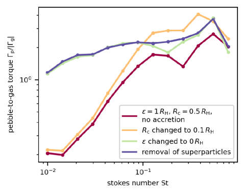
Figure 4: Pebble-to-gas torque as a function of the Stokes number for the planet mass $M_{\mathrm{pl}}=1.51\,M_{\oplus}$. Individual curves track how the torque changes when the key model assumptions are varied one at a time. The red curve corresponds to our superparticle simulations MspE1. The orange curve is obtained by decreasing the material exclusion distance for the torque evaluation to $R_{\mathrm{c}}=0.1\,R_{\mathrm{H}}$. The green curve is obtained by decreasing the potential smoothing length to zero. The blue curve is obtained by removing superparticles below the critical accretion distance and corresponds to the simulation set MspE0. We point out that the shift from the orange to the green curve is caused by the occurrence of pebble-accreting trajectories (such as those shown in the bottom row of Fig. 3), and therefore, the torque-generating asymmetry of the pebble distribution is already affected by pebble accretion even though superparticles are not yet removed from the simulation (this change is shown by the blue curve).

3.4 Role of material exclusion and superparticle removal for the torque evaluation

In Fig. 2, the shift from the first two panels to the bottom one involves several changes of model assumptions, mainly the change in the potential smoothing length $\epsilon$ for pebbles but also the decrease in the cutoff radius, $R_{\mathrm{c}}$, for the torque evaluation (Eq. 12) and the removal of superparticles from the simulation at planetocentric distances $d<3\,R_{\mathrm{surf}}$. One might therefore rightfully wonder which of these changes is the most important for the torque map in the presence of pebble accretion. In this section we try to address this issue by introducing the aforementioned changes one at a time.

Figure 4 shows the pebble-to-gas torque as a function of the Stokes number for the planet mass $M_{\mathrm{pl}}=1.51\,M_{\oplus}$. To guide the eye, we advise the reader to start from the red curve corresponding to the simulation set MspE1. By introducing the decrease in the material exclusion radius from $R_{\mathrm{c}}/R_{\mathrm{H}}=0.5$ to $0.1$, the torque dependence shifts from the red to the orange curve. Then, by decreasing the potential smoothing length from $\epsilon/R_{\mathrm{H}}=1$ to $0$, the torque dependence shifts from the orange to the green curve. Finally, when the removal of superparticles is allowed, we obtain the blue curve corresponding to the simulation set MspE0.

We can see that as long as $\epsilon/R_{\mathrm{H}}=1$, the reduction of the material exclusion radius $R_{\mathrm{c}}$ leads to a substantial boost of the pebble torque only at $\mathrm{St}\gtrsim 0.07$. To boost the torque in the regime of smaller Stokes numbers, it is needed to decrease the potential smoothing to zero, thus enabling the occurrence of pebble-accreting trajectories and the underdense perturbations near the planet.

Introducing the removal of superparticles from the simulation has actually very little influence on the torque. Such a result is not surprising because as long as trajectories that enable pebble accretion are well resolved (which is true for the zero smoothing length, i.e. for the green curve in Fig. 4), they already efficiently remove pebbles from their flux through the Hill sphere and concentrate them near the planet location. A difference would only be observed when relaxing the cutoff radius, $R_{\mathrm{c}}$, even more and thus including fluctuations of the superparticle number density close to the planet in the torque calculation.

The findings of Fig. 4 align well with our previous assertion that pebble accretion has the largest influence on the torque for the smallest considered Stokes numbers. However, having a correct description of pebble dynamics within the Hill sphere (at $\epsilon/R_{\mathrm{H}}=0$) is also important for larger Stokes numbers as it prevents the torque from being overestimated (compare the orange with the green and blue curves at $\mathrm{St}\gtrsim 0.1$).

3.5 Scaling law for the pebble torque

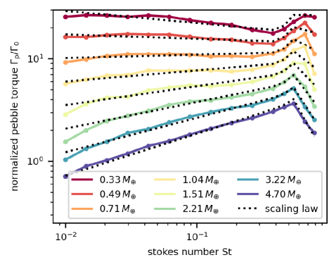
Figure 5: Pebble torque, $\Gamma_{\mathrm{p}}$, normalized by $\Gamma_{0}$ (Eq. 13) as a function of the Stokes number for our superparticle simulations with pebble accretion (set MspE0). Coloured curves distinguish simulation results for different planetary masses, $M_{\mathrm{pl}}$, as specified in the legend. Dotted curves correspond to the empirical scaling law provided in Eqs. (14)–(16) and further generalized in Eqs. (17) and (18).

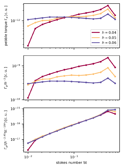
Figure 6: Pebble torque, $\Gamma_{\mathrm{p}}$, acting on a planet with the mass $M_{\mathrm{pl}}=1.51\,M_{\oplus}$ in gas disks with various aspect ratios, $h$. We show the nominal case from the MspE0 simulations with $h=0.05$ (orange), as well as additional calculations for $h=0.04$ (red) and $0.06$ (blue). We compare the dependences for a non-normalized torque (top), a normalization $\Gamma_{\mathrm{p}}/h^{-2}$ following Eq. (13) (middle), and a normalization, $\Gamma_{\mathrm{p}}/(h^{-2.45}\mathrm{St}^{-19h}),$ that we found to be intrinsic to the pebble torque (bottom). The results of the bottom panel were used to generalize our empirical torque formula in Eqs. (17) and (18).

In our simulations with superparticles feeling the unsmoothed gravitational potential of the planet, we have already demonstrated in Fig. 2 that the pebble torque is positive in the entire parameter space and behaves in a regular fashion. This motivated us to search for an empirical scaling law that would allow the pebble torque to be easily incorporated in studies with prescribed migration. These studies involve, but are not limited to, N-body simulations describing the long-term evolution of disk-embedded planetary systems (e.g. Izidoro et al., 2017; Bitsch et al., 2019; Emsenhuber et al., 2021; Matsumura et al., 2021) or simulations of growth tracks of isolated planets within 1D disks (e.g. Bitsch et al., 2015; Johansen et al., 2019).

The gas torque is often normalized with respect to (e.g. Kley & Nelson, 2012)

$$\Gamma_{0}=\left[\Sigma\left(r^{2}\Omega_{\mathrm{K}}\frac{q}{h}\right)^{2}\right]_{\mathrm{pl}}\,,$$ (13)

where $q=M_{\mathrm{pl}}/M_{\star}$ is the planet-to-star mass fraction and the right-hand side is evaluated at the planet’s orbital radius. Various components of the gas torque (often depending on the disk model) either directly follow the functional dependence of $\Gamma_{0}$ (e.g. Tanaka et al., 2002; D’Angelo & Lubow, 2010) or remain similar to it within a factor of a few (e.g. Paardekooper et al., 2011). Guilera et al. (2023), who was the first to include the findings of BLP18 in a global model of planet formation, proposed that the pebble torque is likely to be normalized by $\Gamma_{0}$ as well. In the following, however, we show that Eq. (13) does not fully capture the dependence of $\Gamma_{\mathrm{p}}$ on $q$ and $h$. Nevertheless, we also express the pebble torque as $\Gamma_{\mathrm{p}}/\Gamma_{0}$, simply because it provides a useful reference value when comparing to the gas torque.

We find that the pebble torque exerted on low-mass planets accreting pebbles in the 2D regime can be characterized by the following empirical scaling law

$$\frac{\Gamma_{\mathrm{p}}}{\Gamma_{0}}=\frac{Z}{0.01}\min\left(1.928\times 10^{-3},\xi_{1}(\mathrm{St})\right)q^{\min\left(-0.673,\xi_{2}(\mathrm{St})\right)}\,,$$ (14)

where we defined

$$\xi_{1}(\mathrm{St})=\cases{2}.275\times 10^{-2}{\mathrm{St}}^{2.645}&\mathrm{St}\leq 0.45\,,\\ 9.506\times 10^{-7}{\mathrm{St}}^{-12}\mathrm{St}>0.45\,,\\ {}$$ (15)

$$\xi_{2}(\mathrm{St})=\cases{-}0.479+0.2\log{\mathrm{St}}&\mathrm{St}\leq 0.45\,,\\ -1.241-0.868\log{\mathrm{St}}\mathrm{St}>0.45\,,\\ {}$$ (16)

and $\log$ is the natural logarithm. Figure 5 compares the results of our superparticle simulations MspE0 with the scaling law given by Eqs. (14)–(16) and shows a good agreement.

Returning to the normalization by $\Gamma_{0}$, we split Eq. (13) into three parts. The part $\propto$$\Sigma_{\mathrm{p}}\Omega_{\mathrm{K}}^{2}r^{4}$ is intrinsic to the pebble torque, as we verify in Appendix F. The part $\propto$$q^{2}$ is not intrinsic to the pebble torque: we see in Fig. 5 that measurements of $\Gamma_{\mathrm{p}}/\Gamma_{0}$ for different planet-to-star mass ratios are not aligned,and therefore, the right-hand side of our scaling law (Eq. 14) still depends on $q$.

To investigate the part $\propto$$h^{-2}$, we repeated our superparticle simulations MspE0 with the planet $M_{\mathrm{pl}}=1.51\,M_{\oplus}$ while changing the aspect ratio of the gaseous background to $h=0.04$ and $0.06$. A comparison of the resulting pebble torque is provided in Fig. 6. From the top panel where we plot $\Gamma_{\mathrm{p}}$ directly, it becomes obvious that the torque does not simply scale with a power of $h$. This is further confirmed by the middle panel, where we plot $\Gamma_{\mathrm{p}}/h^{-2}$, which is the normalization dictated by Eq. (13) if only $h$ varies. Clearly, this form of a detrending does not result in an overlap of the measurements. We numerically found that, to achieve the overlap, the normalization should follow $\Gamma_{\mathrm{p}}/(h^{-2.45}\mathrm{St}^{-19h})$, as shown in the bottom panel of Fig. 6. We admit, however, that this normalization starts to fail for the minimum and maximum $\mathrm{St}$ used in our study.

The reason why the dependence on $h$ is relatively complex is because the headwind velocity, to which the dynamics of pebbles is sensitive (Liu & Ormel, 2018), changes with the aspect ratio (see Eq. 3). With the knowledge based on Fig. 6, the scaling law for the pebble torque can be generalized by replacing Eqs. (14) and (15) with

$$\frac{\Gamma_{\mathrm{p}}}{\Gamma_{0}}=\frac{Z}{0.01}h^{-0.45}\min\left(5\times 10^{-4},\xi_{1}(\mathrm{St})\right)q^{\min\left(-0.673,\xi_{2}(\mathrm{St})\right)}\,,$$ (17)

and

$$\xi_{1}(\mathrm{St})=\cases{5}.9\times 10^{-3}{\mathrm{St}}^{3.595-19h}&\mathrm{St}\leq 0.45\,,\\ 2.469\times 10^{-7}{\mathrm{St}}^{-11.05-19h}\mathrm{St}>0.45\,,\\ {}$$ (18)

respectively.

To close the section, we point out that Eqs. (17), (18), and (16) were only tested within the parameter range of our analysis and for $h=0.04$–$0.06$. Whether they can be safely used outside this range or not remains to be verified. Additionally, a caution is needed in situations that would violate our model assumptions (see Sect. 4.5).

4 Discussion

4.1 Pebble torque versus the radial pebble flux

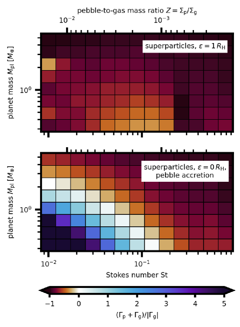
Figure 7: Torque map for a pebble disk characterized by the radial mass flux $\dot{M}_{\mathrm{p}}=10^{-4}\,M_{\oplus}\,\mathrm{yr}^{-1}$. For each Stokes number, $\mathrm{St}$, we obtain $\Sigma_{\mathrm{p}}$ from $\dot{M}_{\mathrm{p}}$ (Eq. 20), which results in the pebble-to-gas mass ratio, $Z,$ decreasing with increasing $\mathrm{St}$, as shown in the upper horizontal axis. The value of $Z$ is used to rescale the results of Fig. 2. We show the total torque (exerted by both pebbles and gas) scaled by the gas-driven torque for simulation sets MspE1 (top) and MspE0 (bottom). In the top panel, the total torque is always negative and planet migration is directed inwards. In the bottom panel, a subset of the parameter space exists for which the total torque is positive, resulting in outward migration.

Our results imply that the positive pebble torque can dominate over the negative gas torque and thus enable outward planet migration in a major portion of the parameter space. One of the key assumptions that enables the pebble torque to become important, and one that has not yet been scrutinized in our study, is the pebble-to-gas mass ratio, $Z$, which we set to 0.01, as in BLP18. Although $Z=0.01$ is a widely adopted canonical value characterizing the dust content in protoplanetary disks, it might not be the best parametrization for pebbles. The population of pebbles inevitably undergoes depletion by the radial drift while, on the other hand, being replenished by coagulation from dust-sized particles. Therefore, it might be more appropriate to parametrize the pebble disk with the radial mass flux $\dot{M}_{\mathrm{p}}$ rather than assuming a fixed value of $Z$.

Lambrechts & Johansen (2014) demonstrated that the typical radial mass flux in pebbles is $\dot{M}_{\mathrm{p}}\simeq 10^{-4}\,M_{\oplus}\,\mathrm{yr}^{-1}$ and the value decreases as the disk evolves. Adopting this finding, we constructed a new migration map as follows. First, for each value of $\mathrm{St}$, we calculated $\Sigma_{\mathrm{p}}$ from the pebble mass flux as outlined in Appendix A and thus obtained a new estimate of $Z(\mathrm{St})=\Sigma_{\mathrm{p}}/\Sigma_{\mathrm{g}}$. The calculation was done at the radial distance $r_{\mathrm{pl}}$ but, as we also show in Appendix A, the resulting value of $Z(\mathrm{St})$ is radially constant in our simple disk model. For $\dot{M}_{\mathrm{p}}=10^{-4}\,M_{\oplus}\,\mathrm{yr}^{-1}$, the upper and lower limits in our parameter space are $Z=1.6\times 10^{-2}$ and $3.2\times 10^{-4}$ for $\mathrm{St}=0.01$ and $0.785$, respectively. The value of $Z$ substantially decreases towards larger Stokes numbers because as the radial drift speeds up, the mass flux conservation dictates a lower surface density. Next, we rescaled each bin of Fig. 2 by a factor of $Z(\mathrm{St})/0.01$ and thus obtained Fig. 7.

The top panel of Fig. 7 corresponding to the simulation set MspE1 reveals that outward migration is no longer possible; the pebble-driven torque can only slow down the rate of inward migration. When pebble accretion is accounted for, on the other hand, the bottom panel of Fig. 7 tells us that outward migration can still occur in the lower-left corner of the map (i.e. roughly for $M_{\mathrm{pl}}\lesssim 1\,M_{\oplus}$ and $\mathrm{St}\lesssim 0.1$). The rate of outward migration increases with decreasing $M_{\mathrm{pl}}$ and $\mathrm{St}$. The main takeaway is that the positive torque enabled for $\mathrm{St}\lesssim 0.1$ by pebble accretion might represent the main channel of pebble-driven migration, given that smaller pebbles are depleted less efficiently by the radial drift.

It is interesting to compare this result with BLP18 and Guilera et al. (2023) who, on contrary, predicted that the pebble torque should dominate and drive outward migration for $\mathrm{St}\gtrsim 0.1$ (the reason for that is immediately visible when going back to the first two panels of Fig. 2). Future assessment based on global models of planet formation is needed to decide whether the predictions of Guilera et al. (2023) hold or become replaced with implications of Fig. 7. Nevertheless, it is clear that the pebble-to-gas mass ratio has to be treated with care to correctly determine situations in which the pebble torque comes into play.

Our discussion only applies to smooth disks in which the radial pebble mass flux is not substantially altered by traffic jams or pressure barriers. However, such dust and pebble concentrations seem to be ubiquitous in realistic protoplanetary disks (Andrews et al., 2018) and might boost the importance of the pebble torque locally, due to the sudden increase in $Z$ (Pierens & Raymond, 2024).

4.2 Possible implications for planet formation

There are three possible implications for planet formation that we would like to highlight. First, it is quite often accepted that gas-driven migration of Mars-sized and smaller planets is extremely inefficient given that its speed decreases linearly with the mass of the migrating body (Tanaka et al., 2002; Morbidelli & Raymond, 2016). On the other hand, the efficiency of the pebble torque relative to the gas torque increases as the planet mass decreases and can reach $\Gamma_{\mathrm{p}}/|\Gamma_{\mathrm{g}}|\sim 10^{1}$. Therefore, unless mitigated by the depletion of pebbles and the decrease in $Z$, the migration rate of these very small planets might become more substantial than usually thought.

Second, we speculate that convergent planet migration might occur at special transition radii at which the properties of pebbles abruptly change. Consider, for instance, the snow line where the water ice sublimates from inward-drifting pebbles. Outside the snow line, pebbles are expected to fragment at velocities $\sim$$10\,\mathrm{m}\,\mathrm{s}^{-1}$ (Poppe et al., 2000; Güttler et al., 2010), whereas they become more fragile as they lose water ice, fragmenting at $\sim$$1\,\mathrm{m}\,\mathrm{s}^{-1}$ (Gundlach & Blum, 2015). Since the size of pebbles scales with the fragmentation velocity squared, it becomes substantially reduced below the snow line. A sharp transition in the pebble size would result in smaller Stokes numbers occurring interior to the snow line (e.g. Morbidelli et al., 2015; Drażkowska & Alibert, 2017; Müller et al., 2021). One can envisage a situation in which Earths and sub-Earths inside the snow line experience the pebble-driven regime of outward migration (as in the lower-left corner of the bottom panel in Fig. 7) but switch to the standard gas-dominated inward migration outside the snow line (by shifting to the orange region of the bottom panel in Fig. 7). The snow line could then become a radius of convergent migration, provided that the radial pebble flux does not decrease too much due to water ice sublimation (Morbidelli et al., 2015). Future works should explore the possibility of such an interplay at various sublimation lines and also at transitions in the turbulent activity of the disk. For instance, the thermal ionization threshold at $T\simeq 900\,\mathrm{K}$ (Desch & Turner, 2015) might enable an efficient magnetorotational instability (Flock et al., 2017) and truncate pebble sizes at $T\gtrsim 900\,\mathrm{K}$, this time due to the increase in turbulent velocities (e.g. Ueda et al., 2019).

Last but not least, there are many examples of global formation models involving pebble accretion in which planets undergo only inward migration throughout the lifetime of their natal disk (e.g. Lambrechts et al., 2019; Johansen et al., 2021). However, the pebble torque can facilitate evolutionary stages of outward migration, having strong implications for the initial formation sites of progenitor planetary embryos or for the material composition inherited by the planets from the disk.

4.3 Pebble torque due to accretion of angular momentum

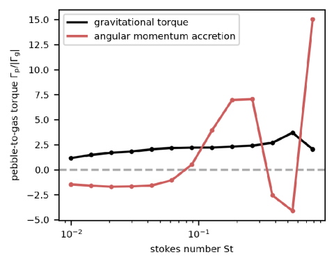
Figure 8: Comparison of the pebble-driven gravitational torque (black) and accretion torque (red; Eq. 19) for the simulation set MspE0 and $M_{\mathrm{pl}}=1.51\,M_{\oplus}$. The two torques seem to have a similar level of importance.

Throughout our study, we only investigated the pebble torque related to the gravitational disk-planet interaction. However, accreted pebbles also carry some amount of angular momentum that might not necessarily match that of the planet. In that case, an additional accretion torque arises, which amounts to

$$\Gamma_{\mathrm{acc}}=(\bar{l}_{\mathrm{acc}}-l_{\mathrm{pl}})\dot{M}_{\mathrm{acc}}\,,$$ (19)

where we define $\bar{l}_{\mathrm{acc}}$ as the average specific angular momentum delivered by accreted pebbles, $l_{\mathrm{pl}}$ as the specific angular momentum of the planet, and $\dot{M}_{\mathrm{acc}}$ as the pebble accretion rate of the planet.

In writing Eq. (19), we assumed that all of the delivered specific angular momentum modifies the orbital momentum of the planet. This is a strong assumption made mainly for convenience and in order to highlight a limit scenario. In reality, the accreted angular momentum might as well modify the spin of the planet (Visser et al., 2020; Takaoka et al., 2023; Yzer et al., 2023). However, what fraction contributes to the spin and what to the orbital momentum remains uncertain.

Fig. 8 compares the accretion torque with the gravitational pebble torque for simulations MspE0, focusing on the planet mass $M_{\mathrm{pl}}=1.51\,M_{\oplus}$. Clearly, $\Gamma_{\mathrm{acc}}$ is substantial. It can negate the effect of $\Gamma_{\mathrm{p}}$ for $\mathrm{St}\lesssim 0.05$ and $\mathrm{St}\simeq 0.35$–$0.55$, or strengthen it for the remaining considered Stokes numbers. In the presence of $\Gamma_{\mathrm{acc}}$, the overall picture presented throughout our paper would change yet again. Therefore, we will direct our future work to investigate the influence of the accretion torque in greater detail, focusing on the final stages of pebble inspiralling towards the planet, which requires the primordial atmosphere to be taken into account (Sect. 4.5).

4.4 Pitfalls of including pebble accretion in 2D multi-fluid simulations

In recent years, several studies have attempted to include pebble accretion in 2D hydrodynamic simulations with multiple fluids (e.g. Chrenko et al., 2017; Regály, 2020; Pierens, 2023). Although different in details, these studies generally define a pebble accretion radius that is typically a large fraction of the Hill radius and then they reduce the surface density of the pebble fluid within this whole radius to match the desired accretion rate of the planet. However, due to the 2D limitation, these studies also employ the smoothing of the planetary gravitational potential for the pebble fluid. In the light of our results, such an approach is dangerous. Consider the first row in Fig. 3 corresponding to multi-fluid simulations with the potential smoothing and imagine that the pebble density is reduced at each time step within a sink area similar to the Hill sphere. This reduced density would be advected back into the disk because there are no streamlines converging at the planet location. There is no guarantee that such a change in the pebble distribution yields a correct torque (any spurious artefact in the front-rear asymmetry of the pebble distribution would change the torque) and therefore, we warn authors against combining the material sink approach with the 2D potential smoothing for pebbles.

4.5 Caveats

In this study, we neglected turbulent dust diffusion and effects of 3D dynamics. This should not be a major obstacle for our choice of $\alpha=10^{-4}$ (see, for instance, Appendix C where we show that the accretion efficiency in a 3D disk would remain similar) but a direct future validation is desirable. We plan to continue our work by extending the Deneb code to 3D. Differences might arise, for example, due to the interaction of pebbles with the recycling flow of low-mass planets (Ormel et al., 2015b; Kuwahara & Kurokawa, 2020), which has no 2D counterpart, or with their primordial atmosphere.

We should also mention that simulations obtained with the Deneb code require that the gas perturbed by the planet is in a steady state and the planet remains deeply embedded. However, reaching a true steady state might be difficult in low-viscosity disks because, given enough time, even low-mass non-migrating planets will eventually carve a small dip around their orbit (e.g. Duffell & MacFadyen, 2013; Ataiee et al., 2018).

Furthermore, we assumed that the Stokes number of pebbles is a constant parameter. It might be more appropriate to fix the physical size of pebbles and calculate the Stokes number self-consistently based on the background gas properties (Epstein, 1924). Additionally, realistic protoplanetary disks contain a broad distribution of pebble and dust sizes, although such a distribution might have a well-defined maximum size containing the majority of the solid mass (e.g. Birnstiel et al., 2012).

We have already mentioned that pebble-accumulating pressure bumps occur in observed disks. The pebble torque might considerably change in such an environment. Pebble distribution near a bump is not governed by inward drift; it instead reaches an equilibrium between convergent drift and divergent spreading by turbulent diffusion (e.g. Dullemond et al., 2018). If a planet finds itself in the inner part of the bump where the gas rotation is super-Keplerian and pebbles undergo outward drift, it is likely that the pebble hole or the dominant underdensity created by pebble accretion would form ahead of the planet. Perhaps the sign of the pebble torque would then flip compared to a smooth sub-Keplerian disk.

Finally, the planet was kept on a fixed circular orbit. Pebble torques acting on migrating planets or planets with excited orbits are yet to be explored. The orbital excitation might in fact occur naturally because pebble accretion can heat up the planet and trigger its eccentricity growth by means of thermal forces (Benítez-Llambay et al., 2015; Eklund & Masset, 2017; Chrenko et al., 2017; Fromenteau & Masset, 2019; Velasco Romero et al., 2022; Chrenko & Chametla, 2023).

5 Conclusions

We have investigated the torque acting on disk-embedded low-mass planets due to the gravitational influence of the surrounding distribution of pebbles. Our main objective was to assess how pebble accretion contributes to the azimuthal asymmetry of the pebble distribution with respect to the planet and hence to the pebble torque. We focused on the 2D limit of pebble accretion, and our parameter space covered planetary masses $M_{\mathrm{pl}}\in[0.33,4.7]\,M_{\oplus}$ and Stokes numbers of pebbles $\mathrm{St}\in[0.01,0.785]$.

First, we used the Fargo3D code to show that the smoothing of the planetary gravitational potential, which is traditionally employed in 2D multi-fluid simulations (; ), prevents pebble accretion from being captured self-consistently. To circumvent this issue, we introduced a new code, Deneb, that approximates pebbles as Lagrangian superparticles evolving in a steady-state gaseous background.

We find that pebble accretion does modify the pebble distribution and influence the torque. When pebbles encounter the planet and some of them are captured by it, the pebble flux after passing through the encounter region is reduced (pebbles are ‘missing’ in the flux). For Stokes numbers $\mathrm{St}\lesssim 0.1$, pebbles from the outer disk first encounter the planet (mostly) from the front, thus forming an underdense region that trails the planet. Pebbles that had already drifted below the planet’s corotation encounter the planet (mostly) from the rear, creating an underdense region in front of the planet. The trailing underdense region is dominant because it is efficiently shielded from the incoming pebble flux, and at the same time it stagnates near the planet’s corotation, where the shear motions reverse.

The paucity of pebbles behind the planet keeps the pebble torque positive and strong, capable of outperforming the gas torque for $M_{\mathrm{pl}}\lesssim 3\,M_{\oplus}$. This was previously thought to be possible for $\mathrm{St}\gtrsim 0.1$ (BLP18), but when pebble accretion is accounted for, the pebble torque starts to dominate planet migration even for small Stokes numbers, $\mathrm{St}\lesssim 0.1$. This finding is important because in protoplanetary disks, there are many situations when pebbles are likely to have small Stokes numbers, either because the disk is still young or because the growth of pebbles is inhibited by various physical barriers (due to the radial drift, fragmentation, bouncing, etc).

Regarding larger pebbles with $\mathrm{St}\gtrsim 0.1$, the main influence of pebble accretion is that there is no sudden change nor reversal in the pebble torque when $\mathrm{St}\simeq 0.3$ (i.e. the transitional regime defined by BLP18, is not present). Similar to the case of smaller pebbles, outward migration is again possible for $M_{\mathrm{pl}}\lesssim 3\,M_{\oplus}$.

All of the above-mentioned conclusions were obtained while assuming a constant pebble-to-gas mass ratio of $Z=0.01$. When the pebble population is instead characterized by a uniform radial mass flux of $\dot{M}_{\mathrm{p}}=10^{-4}\,M_{\oplus}\,\mathrm{yr}^{-1}$ (Lambrechts & Johansen, 2014), outward migration is possible for $M_{\mathrm{pl}}\lesssim 1\,M_{\oplus}$ and $\mathrm{St}\lesssim 0.1$ but seems unlikely for $\mathrm{St}\gtrsim 0.1$ (Sect. 4.1).

We have provided a scaling law for the pebble torque (Eqs. 17, 18, and 16) that is valid in the aforementioned range of parameters and in 2D locally isothermal disks. This scaling law can be used for a straightforward inclusion of pebble-driven migration in global models of planet formation with prescribed migration rates.

We have also shown that the accretion of angular momentum carried by pebbles, in addition to the gravitational torque, can modify planet migration (Sect. 4.3) and deserves to be studied in detail in follow-up studies.

Appendix A Uniform radial mass flux of pebbles

In this appendix we show that the initial state of the pebble disk in our models exhibits a uniform radial mass flux $\dot{M}_{\mathrm{p}}=\mathrm{const}$. The pebble surface density relates to the mass flux as

$$\Sigma_{\mathrm{p}}=-\frac{\dot{M}_{\mathrm{p}}}{2\pi ru_{r}}\,.$$ (20)

The radial velocity of pebbles (Eq. 6) can be approximated as

$$u_{r}\simeq-2\frac{\mathrm{St}}{1+\mathrm{St}^{2}}\eta v_{\mathrm{K}}\,.$$ (21)

For a gas disk with $h=\mathrm{const}$ in a locally isothermal approximation, $P$ is a power-law function of $r$ and thus $\eta\propto(r/P){\partial P}/{\partial r}=\mathrm{const}$ (see Eq. 3). In our study, we additionally considered $\mathrm{St}=\mathrm{const}$ (the Stokes number is only varied between individual simulations as a parameter), which yields $u_{r}\propto r^{-1/2}$. Putting everything together, it is clear that $\dot{M}_{\mathrm{p}}=\mathrm{const}$ is satisfied whenever

$$\Sigma_{\mathrm{p}}\propto r^{-1/2}\,,$$ (22)

which corresponds to our initial conditions specified in Eqs. (1) and (4).

On the other hand, if the pebble disk is initially parametrized by $\dot{M}_{\mathrm{p}}$, the same line of reasoning tells us that $Z=\Sigma_{\mathrm{p}}/\Sigma_{\mathrm{g}}=\mathrm{const}$ in our disk model. This fact is utilized in Sect. 4.1.

Appendix B Removing boundary artefacts in the superparticle distribution

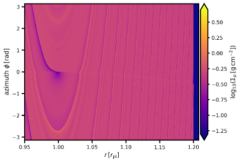
Figure 9: Global view of the time-averaged surface density of pebbles in the simulation MspE0_M1.5St0.089 without (top) and with (bottom) the addition of random noise to the gas velocities near the outer truncation of the superparticle domain. The bottom panel correctly recovers the underdense perturbation created by pebble accretion and pebble dynamics near the planet while avoiding the disturbances spreading from the outer boundary.

In Sect. 2.2 we specified that we employed a narrow patch near the outer boundary of our simulations with superparticles in which we added random noise to the underlying gas velocities. Figure 9 shows the same simulation MspE0_M1.5St0.089 performed without and with the noise (top and bottom panels, respectively). When the noise is absent, one can see that the time-averaged surface density develops a dent near the outer boundary $r_{\mathrm{max}}=1.2\,r_{\mathrm{pl}},$ where we introduce new superparticles in the simulation. The dent is related to the velocity kink that pebbles experience when crossing the gaseous outer spiral wake. Consequently, a set of stripes spreads from the dent by the radial drift and plagues the solution in the domain of interest. There is a risk that the stripes might cross the planetary orbit near $\varphi_{\mathrm{pl}}=0$ and affect the torque measurement. However, it is clear that when the noise zone is considered, the stripes spreading from the outer truncation of the superparticle distribution are efficiently erased and the aforementioned problem with the torque evaluation is avoided.

Appendix C Verification of accretion rates obtained with the Deneb code

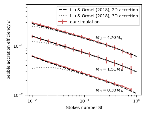
Figure 10: Pebble accretion efficiency, $\mathcal{E,}$ as a function of the Stokes number, $\mathrm{St,}$ for three values of planet mass, $M_{\mathrm{pl}}$, across our parameter range. We compare numerical measurements obtained with our Deneb code (red points and segments) with the scaling laws appropriate for the 2D (dashed black curve) and 3D (dotted grey curve) regimes of pebble accretion (Liu & Ormel 2018). The error bars around the red points correspond to the Poisson counting uncertainties.

Our code Deneb introduced in Sect. 2.2 has been developed specifically for this study and it is only appropriate to present its validation tests. One proof of validity is presented in Fig. 2 where the first two panels compare the pebble torques resulting from Fargo3D simulations with the outcome of Deneb. Another proof is provided in Fig. 3 where the particle trajectories are indistinguishable from pebble fluid streamlines as long as $\mathrm{St}$ is low and $\epsilon$ is the same. Here we focus on the measurement of pebble accretion rates obtained with our new code. More specifically, we followed Liu & Ormel (2018) and measured the accretion efficiency $\mathcal{E}_{\mathrm{2D}}=\dot{M}_{\mathrm{acc}}/\dot{M}_{\mathrm{p}}$, where $\dot{M}_{\mathrm{acc}}$ is the pebble accretion rate.

The results are presented in Fig. 10, where we plot $\mathcal{E}_{\mathrm{2D}}$ as a function of $\mathrm{St}$ for three different planetary masses $M_{\mathrm{pl}}$. The measurement was performed as follows. We initialized $10^{3}$ particles (or $10^{4}$ particles for the lowest considered planet mass) at the radial distance $r=r_{\mathrm{pl}}+10R_{\mathrm{H}}$ uniformly along the whole azimuth. We then integrated the particle trajectories until they either became accreted by the planet or they crossed $r=r_{\mathrm{pl}}-2R_{\mathrm{H}}$ due to their radial drift. The efficiency $\mathcal{E}_{2D}$ was computed directly as the fraction of particles that hit the planet. As our intention was to compare the resulting $\mathcal{E}_{\mathrm{2D}}$ with Liu & Ormel (2018), we azimuthally averaged the gas velocities $v_{\varphi}$ and set $v_{r}=0$ because Liu & Ormel (2018) did not account for perturbations of gas induced by the planet.

The results of Fig. 10 reproduce the scaling law of Liu & Ormel (2018) very well (within the margins of the Poisson counting errors). Furthermore, we plot the 3D accretion rate $\mathcal{E}_{\mathrm{3D}}$ (Liu & Ormel 2018; Ormel & Liu 2018) to compare it with the 2D approximation. In the 3D accretion formula, we considered the vertical scale height of pebbles (Dubrulle et al. 1995)

$$H_{\mathrm{p}}=\sqrt{\frac{\alpha}{\alpha+\mathrm{St}}}H_{\mathrm{g}}\,.$$ (23)

We can see that since the disk viscosity $\alpha=10^{-4}$ adopted in our models is low, the resulting turbulent stirring of the pebble disk would be relatively weak and thus the 3D feeding zone of the planets would encapsulate the majority of the vertical height of the pebble layer, making 2D and 3D accretion rates compatible in the explored range of Stokes numbers $\mathrm{St}\in[0.01,0.785]$. The largest difference is found for $M_{\mathrm{pl}}=0.33\,M_{\oplus}$ and $\mathrm{St}=0.01$, predicting the 2D accretion rate by a factor of $\simeq$$1.8$ larger than the 3D accretion rate.

Appendix D Comparison of the Deneb and Dusty FARGO-ADSG codes

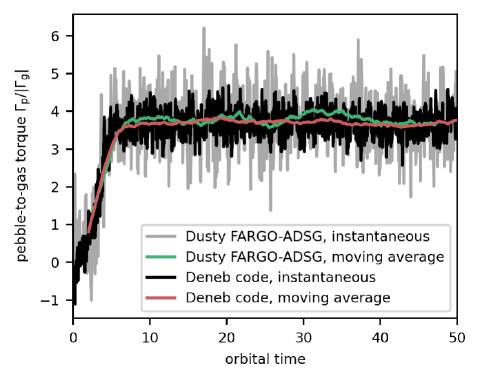
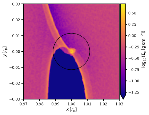
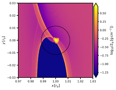
Figure 11: Comparison between the Dusty FARGO-ADSG and Deneb codes for the simulation MspE0_M1.5St0.546. We show the time evolution of the pebble-to-gas torque, $\Gamma_{\mathrm{p}}/|\Gamma_{\mathrm{g}}|,$ over 50 orbital periods (top) and the time-averaged pebble surface density, $\Sigma_{\mathrm{p}}$, after simulating 50 orbital periods with Dusty FARGO-ADSG (middle) and 200 orbital periods with Deneb (bottom).

As our final validation test of the Deneb code, we performed a comparison with Dusty FARGO-ADSG (Baruteau & Zhu 2016), which is a 2D hybrid fluid-particle code as well. However, Dusty FARGO-ADSG evolves the gas and pebbles simultaneously, with the time-step size being controlled by the Courant-Friedrichs-Lewy condition appropriate for the studied system. Additional differences of our Dusty FARGO-ADSG runs include:

• A semi-implicit first-order Euler orbital integrator (similar to Zhu et al. 2014) is used to evolve superparticles.

• Interpolation back and forth between the grid-based quantities and their counterparts at superparticle locations is achieved using a triangular-shaped cloud method.

• The grid resolution is lower, $N_{r}\times N_{\varphi}=1200\times 12288$.

• The number of superparticles is lower, $N_{\mathrm{sp}}=10^{6}$.

• The replenishment of superparticles at $r_{\mathrm{max}}$ is slightly different; each superparticle that becomes accreted or drifts below $r_{\mathrm{min}}$ becomes immediately revived at $r_{\mathrm{max}}$.

• The distance from the planet below which superparticles are accreted is larger, equal to $0.03\,R_{\mathrm{H}}$.

Figure 11 compares the torque evolution and time-averaged pebble surface density between Dusty FARGO-ADSG and Deneb for the simulation MspE0_M1.5St0.546 (corresponding also to the last panel of Fig. 3). The match between the torque, as well as between the main features of the pebble distribution, is satisfactory and tells us that:

• The results obtained with Deneb are robust against specific choices of methods listed above (e.g. the orbital integrator or the interpolation method).

• Our assumption of the gas distribution being non-evolving in Deneb is valid for the physical model that we have considered.

• High resolution and high number of superparticles is beneficial to reduce the noise of the torque measurements and resolve fine details in the pebble distribution.

Appendix E Peculiar pebble traps in the presence of the smoothed planet potential

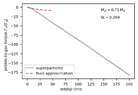
Figure 12: Temporal evolution of the pebble-to-gas torque for simulations MfaE1_M0.7St0.264 (dashed red curve) and MspE1_M0.7St0.264 (grey curve). The linear decrease in the pebble torque is directly related to the accumulation of pebbles in a filament trailing the planet (see Fig. 13).

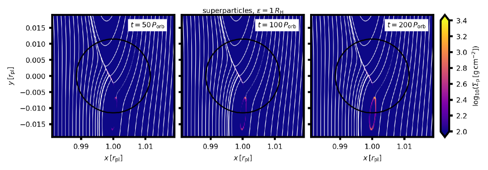
Figure 13: Evolution of the time-averaged surface density, $\Sigma_{\mathrm{p}}$, in the simulation MspE1_M0.7St0.264. The time is given by a label in each panel. The colour palette is saturated in order to highlight how the overdensity of the filament encircling the pebble hole increases in time as more and more pebbles become trapped. A representative trajectory entering the overdense region is shown with a dotted curve and then truncated in order to keep the filament visible. The filament generates a strong negative torque (see Fig. 12).

Having a deeper understanding of the typical sub-structures in the pebble distribution that drive the torque (Sect. 3.3), here we examine one of the cases corresponding to the transitional regime (defined in BLP18, ) for which the simulation sets MfaE1 and MspE1 disagreed. The simulation parameters were $M_{\mathrm{pl}}=0.71\,M_{\oplus}$ and $\mathrm{St}=0.264$ (simulations marked with crosses in Fig. 2).

Figure 12 shows the pebble-to-gas torque recorded in the respective simulations. We can see that although the pebble torque is negative in both cases, it does show signs of convergence in the fluid approximation while it steadily continues to decrease in the superparticle approximation. At the end of the superparticle simulation, the pebble torque exceeds the gas torque by more than two orders of magnitude, which would of course trigger fast inward migration of the planet.

The persistent decrease in the pebble torque shown in Fig. 12 suggests that there must be an overdensity of pebbles trailing the planet and that this overdensity traps more and more pebbles as the simulation progresses. Furthermore, since the decrease in the torque only appears for the superparticle simulation, we expect the overdensity to be related to structures at the resolution limit of the underlying grid. We point out that BLP18 already reported that a very large resolution is needed to properly capture the torque behaviour in the transitional regime.

Indeed, this is confirmed in Fig. 13, which shows the time evolution of the pebble surface density in the superparticle simulation. We can see that the density of the filament encircling the pebble hole grows in time, explaining why the torque becomes ever more negative. The peak density in the filament at the end of the simulation is huge, reaching $\Sigma_{\mathrm{p}}\simeq 2500\,\mathrm{g}\,\mathrm{cm}^{-2}$ and $Z\simeq 50$. The filament is very thin compared to the cell sizes of the underlying polar grid, which is why the fluid approximation leads to an underestimation of the local density accumulation.

Dynamical effects that can trap pebbles are of increased importance in the field of planet formation because they can promote further coagulation-fragmentation cascade in the local size distribution, gas-dust instabilities, or even a collapse into larger objects. Nevertheless, it is questionable whether the interplay described above is realistic. First, it occurs when pebbles feel the smoothed planetary potential, which, as we argued, is undesired for pebble accretion. Second, it completely breaks our model assumptions. Since the solid-to-gas ratio increases by several orders of magnitude, the aerodynamic back-reaction of pebbles on the gas cannot be ignored anymore. Similarly, because the torque on the planet is strong, the whole interplay should be studied with a moving planet, not a fixed one. Finally, it is likely that even a small level of turbulent diffusion would reduce the amount of trapped pebbles, given the sharp density gradient and the small spatial scale on which it occurs across the filament. We leave these investigations for future work.

Appendix F Pebble torque normalization

In this appendix we explore whether the pebble torque can be intrinsically normalized with a factor $\propto$$\Sigma_{\mathrm{p}}\Omega_{\mathrm{K}}^{2}r^{4}$, which represents a part of the quantity $\Gamma_{0}$ introduced in Eq. (13). To verify that, we repeated the simulations MfaE1 with a $M_{\mathrm{pl}}=1.51\,M_{\oplus}$ planet but we shifted the planet to $r_{\mathrm{pl}}=20.8\,\mathrm{au}$. Then we compared the resulting torque normalized as $\Gamma_{\mathrm{p}}/(\Sigma_{\mathrm{p}}\Omega_{\mathrm{K}}^{2}r^{4})$ with our nominal measurement at $r_{\mathrm{pl}}=5.2\,\mathrm{au}$. Figure 14 depicts this comparison for our range of Stokes numbers and validates the normalization, at least for the model assumptions adopted in our study.

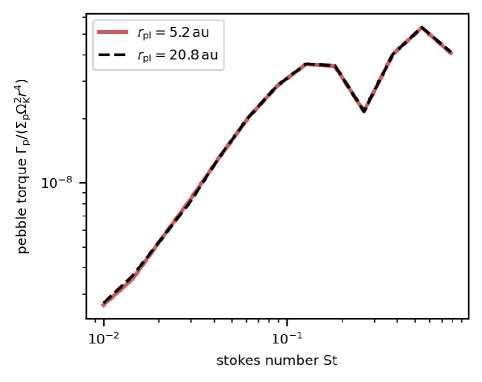
Figure 14: Pebble torque normalized as $\Gamma_{\mathrm{p}}/(\Sigma_{\mathrm{p}}\Omega_{\mathrm{K}}^{2}r^{4})$ for two different radial distances of the planet. The fluid approximation for pebbles is used, corresponding to the model MfaE1. The overlap of the measurements suggests that this normalization is intrinsic to the pebble torque.