Mapping the longitudinal magnetic field in the atmosphere of an active region plage
from the inversion of the near-ultraviolet CLASP2.1 spectropolarimetric data

Abstract

We apply the HanleRT Tenerife Inversion Code to the spectro-polarimetric observations obtained by the Chromospheric LAyer SpectroPolarimeter. This suborbital space experiment measured the variation with wavelength of the four Stokes parameters in the near-ultraviolet spectral region of the Mg II h & k lines over a solar disk area containing part of an active region plage and the edge of a sunspot penumbra. We infer the stratification of the temperature, the electron density, the line-of-sight velocity, the micro-turbulent velocity, and the longitudinal component of the magnetic field from the observed intensity and circular polarization profiles. The inferred model atmosphere shows larger temperature and electron density in the plage and the superpenumbra regions than in the quiet regions. The shape of the plage region in terms of its brightness is similar to the pattern of the inferred longitudinal component of the magnetic field in the chromosphere, as well as to that of the overlying moss observed by AIA in the 171 Å band, which suggests a similar magnetic origin for the heating in both the plage and the moss region. Moreover, this heating is particularly significant in the regions with larger inferred magnetic flux. In contrast, in the superpenumbra, the regions with larger electron density and temperature are usually found in between these regions with larger magnetic flux, suggesting that the details of the heating mechanism in the chromosphere of the superpenumbra may be different to those in the plage, but with the magnetic field still playing a key role.

1 Introduction

The solar chromosphere is an extended region above the photosphere where the magnetic pressure overcomes the gas pressure and dominates the dynamic and structure of the solar plasma (e.g., the review by Carlsson et al., 2019, and references therein). Unveiling and understanding the magnetism of the solar chromosphere is key to discern how the magnetic energy is transported to, and dissipated in, the chromosphere and the transition region.

Our primary means to obtain empirical information on the solar magnetic field is via the inversion of the polarized spectra of atomic lines (e.g., the reviews by del Toro Iniesta & Ruiz Cobo, 2016; Lagg et al., 2017; de la Cruz Rodríguez & van Noort, 2017). Among the spectral lines forming in the upper solar chromosphere, strong ultraviolet (UV) lines such as H I Ly$\rm\alpha$ and the Mg II h and k lines are considered promising for magnetic field diagnostics (Trujillo Bueno et al. 2011, 2012; Belluzzi & Trujillo Bueno 2012; Belluzzi et al. 2012; Štěpán et al. 2015; Alsina Ballester et al. 2016; del Pino Alemán et al. 2016, 2020; Trujillo Bueno et al. 2017, and Judge et al. 2022). However, acquiring the necessary UV spectro-polarimetric observations and inferring the magnetic field from them is a rather challenging task (e.g., the review by Trujillo Bueno & del Pino Alemán, 2022).

The sounding rocket experiments Chromospheric Lyman-Alpha SpectroPolarimeter (CLASP; Kobayashi et al., 2012; Kano et al., 2012) and Chromospheric LAyer SpectroPolarimeter (CLASP2; Narukage et al., 2016; Song et al., 2018) successfully observed the H I Ly$\rm\alpha$ intensity and linear polarization in the quiet sun (Kano et al., 2017; Trujillo Bueno et al., 2018) and the Mg II h and k full Stokes parameters in both a quiet region close to the solar limb (Rachmeler et al., 2022) and a plage region (Ishikawa et al., 2021), respectively (see also Ishikawa et al. 2023). By applying the weak field approximation (WFA), Ishikawa et al. (2021) produced a map of the longitudinal component of the magnetic field across the solar atmosphere, from the photosphere to the upper chromosphere just below the transition region. Moreover, Li et al. (2023) applied the HanleRT Tenerife Inversion Code (hereafter, HanleRT-TIC) to invert the same data, obtaining a stratification of the temperature, electron density, line of sight velocity, micro-turbulent velocity, gas pressure, and the longitudinal component of the magnetic field at each location along the slit, confirming and extending the results obtained by applying the WFA and further allowing for a rough estimation of the energy that could be carried by Alfvén waves propagating across the plage region chromosphere, which exceeded the expected radiative losses.

The success of these suborbital space experiments motivated the third CLASP mission, the second flight of the Chromospheric LAyer SpectroPolarimeter (CLASP2.1). Instead of sit-and-stare observations, the CLASP2.1 scanned a two dimensional field of view of an active region plage measuring the wavelength variation of the four Stokes parameters in the same spectral region as the CLASP2 , i.e. from $\sim$279.30 to $\sim$280.68 nm including the Mg II h and k lines.

Due to the formation height of the Mg II h and k lines, the CLASP2.1 observation provides an opportunity to investigate the heating processes in the upper chromosphere, close to the base of the transition region to the corona. However, partial frequency redistribution (PRD) effects and atomic level polarization induced by the scattering of anisotropic radiation must be taken into account, even to model just their circular polarization (Alsina Ballester et al., 2016; del Pino Alemán et al., 2016). These physical ingredients do not only add complexity to the the inversion of the Mg II h and k lines, but also significantly increase the computational cost. In this work, we apply the HanleRT-TIC to invert these spectro-polarimetric data and obtain the stratification of the temperature, electron density, line-of-sight (LOS) velocity, micro-turbulent velocity, and the longitudinal component of the magnetic field in the middle and upper chromosphere. To reduce the computing cost, we use a relative simple four-level Mg model atom, which includes only the h and k lines. The model parameters resulting from the inversion provide insights on the heating processes in the chromosphere and the overlying corona.

2 Observation

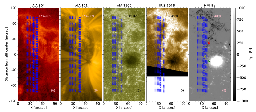
Figure 1: AIA images in the 304 (A), 171 (B), and 1600 Å (C) bands. (D) IRIS slit-jaw image at 2796 Å. (E) HMI magnetogram. Panels (A), (B), and (C) are shown in log scale. The blue vertical lines indicate the 16 slit positions in the CLASP2.1 observation. The red, yellow, and green “$\times$” symbols in panel (E) indicate the position of the example profiles shown in Figs. 3, 8, and 10–12.

The spectro-polarimetric data correspond to a spectrograph slit scan of NOAA AR 12882 performed by the CLASP2.1 suborbital experiment on 8 October 2021. The target active region was close to the disk center, with a heliocentric angle $\theta$ such that $\rm\cos{\theta}\sim 0.9$. The scanning consists of 16 slit positions, acquired between 17:42:13 and 17:47:38 UT, with an exposure time of about 18 s which was slightly different for each slit position. The spatial resolution along the slit direction is 0.53 arcsec/pixel. The slit raster step is about 1.8 arcsec on average.

The field of view covers a plage region and the edge of a sunspot penumbra, with the same spectral range and resolution as the CLASP2, i.e. from $\sim$279.30 to $\sim$280.68 nm with a spectral sampling of 49.9 mÅ/pixel, and a spectral point spread function which can be approximated by a gaussian with a full width at half maximum (FWHM) of about 110 m${\rm\AA}$ (Song et al., 2018; Tsuzuki et al., 2020). The full Stokes spectro-polarimetric observation includes, among other atomic lines, the Mg II h and k lines, the two blended subordinate lines of the Mg II at 279.88 nm, and three Mn I resonance lines at 279.56, 279.91, and 280.19 nm. The wavelength is calibrated by assuming that the Mn I lines are at rest. Therefore, the inferred longitudinal velocity values are relative to the lower chromosphere, where the Mn I lines are formed. The polarimetric accuracy is abount $10^{-3}$ at the intensity peaks of the Mg II h and k lines, which is slightly worse than that in the CLASP2 observations due to the shorter integration time at each slit position, but still sufficient to apply the HanleRT-TIC in order to estimate the chromospheric magnetic field in the target region from the observed Stokes $I$ and $V$ profiles.

Observations of the target region obtained by the Atmospheric Imaging Assembly (AIA; Lemen et al., 2012) on board the Solar Dynamic Observatory (SDO; Pesnell et al., 2012) are shown in Fig. 1. The blue vertical lines in the figure indicate the 16 slit positions, which cover a region of the active region plage and the edge of the sunspot penumbra. A moss region (Berger et al., 1999) located near the footpoints of some coronal loops can be seen in the 171 Å band approximately in the ranges 10 – 60  arcsec in the X direction and 20 – 100 arcsec in the Y direction. The moss region also presents emission features in the 304 Å band. Coordinated observations of the same active region were acquired by the Interface Region Imaging Spectrograph satellite (IRIS; De Pontieu et al., 2014) and the Helioseismic and Magnetic Imager (HMI; Schou et al., 2012).

3 Inversion strategy

Table 1: Number of nodes in the temperature ($T$), micro-turbulent velocity ($v_{\rm turb}$), vertical velocity ($v_{z}$), gas pressure ($P_{\rm g}$), and vertical component of the magnetic field ($B_{z}$) for each inversion cycle. Zero nodes indicate that the variable is fixed to the value resulting from the last cycle (or that it is set to zero if it is the first cycle). The single node in $P_{\rm g}$ indicates that only its value at the top boundary is a free parameter and its stratification is obtained from the assumed hydrostatic equilibrium.

cycle	$T$	$v_{\rm turb}$	$v_{z}$	$P_{\rm g}$	$B_{z}$
1	4	3	3	1	0
2	7	5	4	1	0
3	0	0	0	0	1
4	0	0	0	0	4

Figure 2: Intensity at $\rm k_{2b}$ (first column), $\rm h_{3}$ (second column), and $\rm h_{1r}$ (third column), and circular polarization at $\rm k_{3}$ (fourth column), $\rm k_{1r}$ (fifth column), and $\rm h_{2b}$ (sixth column) for the observation (top row) and the inversion fit (bottom row). The wavelengths corresponding to $\rm k_{2b}$, $\rm h_{3}$, $\rm h_{1r}$ $\rm k_{3}$, $\rm k_{1r}$, and $\rm h_{2b}$ are indicated with colored dashed lines in Fig. 3. The units for Stokes $I$ and $V$ are the same as in Fig. 3.

In this paper we use the HanleRT-TIC, a non-local thermodynamical equilibrium Stokes inversion code, which solves the radiative transfer problem assuming one-dimensional plane-parallel geometry. Hydrostatic equilibrium is assummed to compute the stratified gas pressure from that at the top boundary (Mihalas, 1978). The atomic and electron number densities are calculated by solving the equation of state in local thermodynamic equilibrium with the method of Wittmann (1974). The code takes into account PRD effects (in this paper we use the angle-averaged formalism, see, e.g., Mihalas 1978; Leenaarts et al. 2012; Belluzzi & Trujillo Bueno 2014), $J$-state interference, and atomic level polarization in the incomplete Paschen-Back regime following the formalism in Casini et al. (2014, 2017a, 2017b). Note that the atomic level polarization and the radiation field anisotropy significantly impact the circular polarization of the outer lobes of the Mg II h and k line profiles (Alsina Ballester et al., 2016; del Pino Alemán et al., 2016).

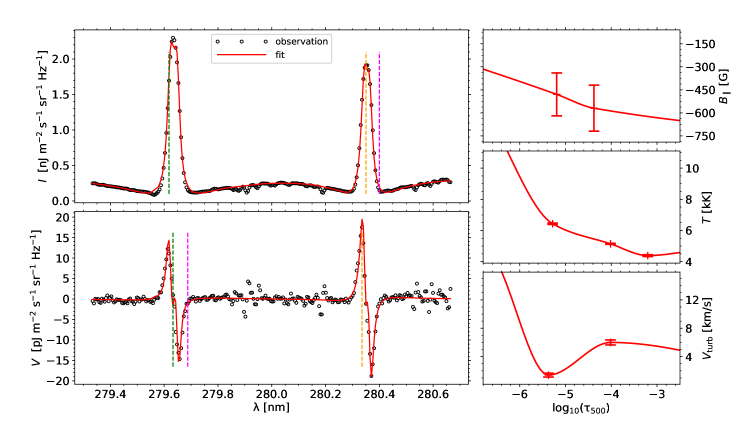
Figure 3: Observed (open circles) and fitted (red solid curve) intensity (top left panel) and circular polarization (bottom left panel) profiles for a pixel in the plage (red “$\times$” symbol in Panel (E) of Fig. 1). Inferred $B_{\parallel}$, $T$, and $v_{\rm turb}$ are shown in the right panels, from top to bottom, respectively. The ${\rm k_{1b}}$ minimum (at around 279.57 nm) is blended with a Mn I line, and those frequency nodes are not present in the inversion (thus resulting in a straight line in the plot). The green, orange, and purple dashed lines in the top left panel indicate the wavelength location of ${\rm k_{2b}}$, ${\rm h_{3}}$, and ${\rm h_{1r}}$, respectively. The green, orange, and purple dashed lines in the bottom left panel indicate the wavelength location of ${\rm k_{3}}$, ${\rm h_{2b}}$, and ${\rm k_{1r}}$, respectively.

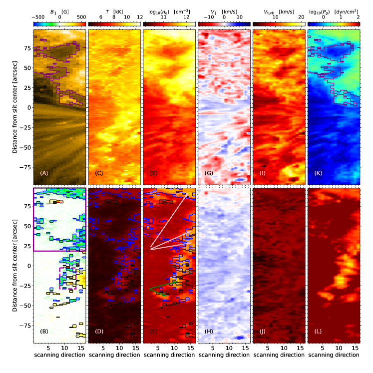
Figure 4: Top left panel: AIA image in the 171 Å band. Bottom left panel: HMI magnetogram (corresponding color bar at the top of the top-left panel). From the second to the sixth columns: Inferred temperature, electron density, longitudinal component of the velocity, micro-turbulent velocity, and gas pressure at ${\rm log_{10}}(\tau_{500})=-6.0$ (top panels) and ${\rm log_{10}}(\tau_{500})=-4.5$, (bottom panels). Purple contours in panels (A) and (K) are drawn according to the intensity of the 171 Å AIA band. Black and blue contours in panels (B), (D), and (F) correspond to the HMI magnetic field values of 70 G and $-70$ G, respectively. In panel (B), the squares drawn with solid and dashed purple lines delimit the pixels included in the scatterplots in Fig. 5 (see text). The white and green arrows highlight regions of the field of view discussed in the text.

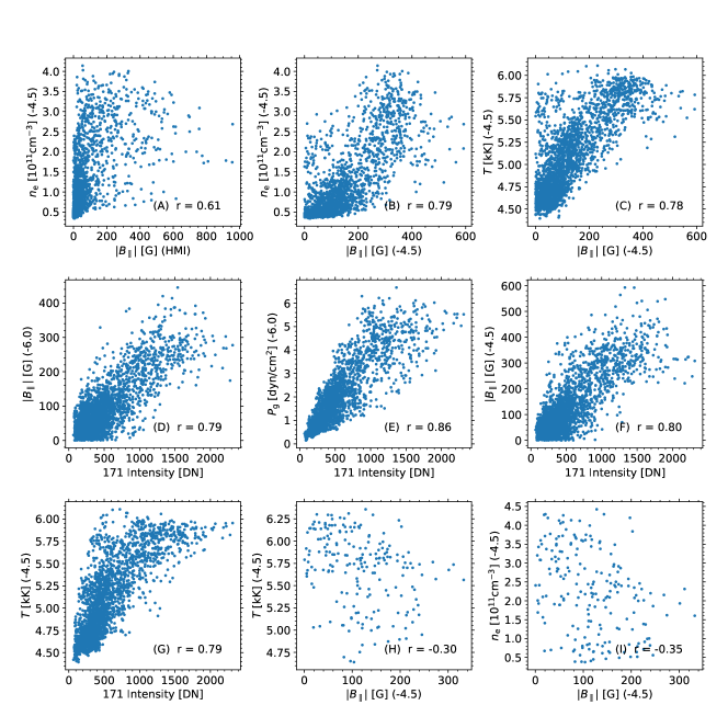
Figure 5: Scatterplots for selected parameter pairs. In the labels, the number between parenthesis indicate the $\log_{10}(\tau_{500})$ where the value of the variable is taken from the inversion result, “(HMI)” indicates that the value is taken from the HMI magnetogram, and the label “171 Intensity [DN]” indicates the intensity in the AIA 171 Å band. The points in panels (A) – (G) correspond to the region delimited by solid purple lines in the bottom-left panel of Fig. 4, while the points in panels (H) and (I) correspond to the region delimited by the dashed purple lines in the same panel of Fig. 4. The Pearson correlation coefficient is shown in each panel.

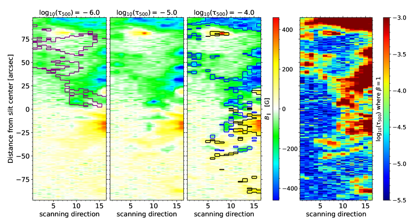
Figure 6: Inferred $B_{\parallel}$ at ${\rm log_{10}}(\tau_{500})=-6.0$, $-5.0$, and $-4.0$ (three left panels, from left to right, respectively). The rightmost panel shows the height where the plasma $\beta=1$ (assuming the magnetic field is parallel to the LOS). Contour curves are the same as in Fig. 4.

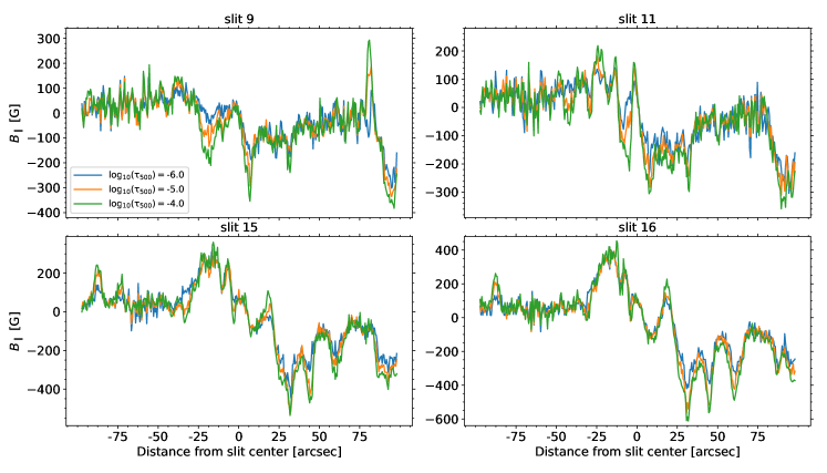
Figure 7: Inferred $B_{\rm\parallel}$ at ${\rm log_{10}}(\tau_{500})=-6.0$ (blue curves), $-5.0$ (orange curves), and $-4.0$ (green curves) for slit locations 9, 11, 15, and 16 (see label on top of the panels). The slit positions on the observation field of view are indicated by the blue dashed curves in Fig. 1.

We applied an inversion strategy similar to that outlined in Li et al. (2023), namely two non-magnetic cycles to obtain the thermodynamic model, i.e., temperature ($T$), LOS velocity ($v_{\parallel}$), micro-turbulent velocity ($v_{\rm turb}$), and gas pressure ($P_{\rm g}$), from just the intensity profile. The model atmosphere used in the spectral synthesis is stratified with 60 non-equally spaced layers between ${\rm log_{10}}(\tau_{500})=-8.0$ and 1.0. In order to reduce the significant computational requirements, once the Stokes $I$ inversion is completed, we fix the thermodynamic quantities of the model and we only invert the longitudinal magnetic field ($B_{\parallel}$) from the observed circular polarization in two cycles. As in Li et al. (2023), the plasma velocity and the magnetic field are assumed to be parallel to the local vertical in the inversion, since the non-axial symmetric components of the velocity and the magnetic field significantly increase the computing time, without significantly impacting the circular polarization for the LOS of the observation. The vertical components ($v_{z}$ and $B_{z}$) are then projected onto the LOS, and these longitudinal components are the ones constrained by the observation. In Table 1 we show the number of nodes for each variable in each cycle. In addition, it is only in the last cycle that we take the radiation field anisotropy into account. In this paper we only show the nodes of the inversion between ${\rm log_{10}}(\tau_{500})=-6.8$ and $-2.5$. During the inversion we also considered two nodes at ${\rm log_{10}}(\tau_{500})=-8.0$ and $1.0$, at the top and bottom boundaries of the model atmosphere, respectively. Moreover, for the temperature we considered an additional node at around ${\rm log_{10}}(\tau_{500})=-1.8$. This node selection was the result of experimentation with the inversion of the intensity profiles.

The errors in the inferred parameters are computed from the diagonal of the Hessian matrix (e.g. del Toro Iniesta, 2003). The uncertainties given by this method indicate how well contrained a node value is relative to the others (Milić & van Noort, 2018). One of the best ways to estimate the confidence interval of the inferred node values is via Bayesian inference by implementing a Markov chain Monte Carlo (e.g., Asensio Ramos et al., 2007; Li et al., 2019). However, more than $10^{5}$ synthesis are typically required to achieve a good posterior distribution, and thus this approach is suitable for very fast forward models. Besides these two methods, Monte Carlo simulations have also been used to estimate uncertainties (Westendorp Plaza et al., 2001; Sainz Dalda & De Pontieu, 2023). In this method random noise is added to the Stokes profiles, and the standard deviation of the results of the inversion of these profiles is representative of the uncertainty. An example of the uncertainty estimated using this method is shown in Sec. 4.3. Note that all the uncertainties mentioned above are representative of how the inferred parameters can change without significantly impacting the merit function of the inversion, i.e., the measurement of the goodness of the fit.

In the spectral region observed by the CLASP2.1 there are three resonance lines of Mn I at 279.56, 279.91, and 280.19 nm, as well as two blended lines of Mg II at 279.88 nm. Including these transitions in the inversion helps contraining the inference in the upper photosphere and lower chromosphere. However, we have found that, for these data, the results of the inversion of the Mg II h and k lines including and neglecting these other lines are compatible within the inversion errors. Therefore, to ease the already significant computational cost, we have performed the inversions pixel by pixel using a Mg II model atom with four levels, the lower and upper levels of the Mg II h and k lines and the Mg III ground level. We show the comparison between the inversions including and neglecting the Mg II UV triplet and the Mn I resonance lines in Appendix A.

Fig. 2 shows observations of the Stokes $I$ and $V$ signals at the wavelengths indicated in the caption and the fits resulting from the inversions. Overall the fits present the main features of the observation both at the line center and in the wings. The fits of the circular polarization are smoother than the observation, which is expected due to the polarization noise of the observation.

4 Results

In this section we show the results of the inversion of the CLASP2.1 data following the strategy described in Sec. 3. In particular we emphasize the inversion results in the plage region (Sec. 4.1), the penumbra and superpenumbra (Sec. 4.2), and in a region where we find a change of the magnetic field polarity with height (Sec. 4.3).

4.1 The plage and the overlying moss

The plage region observed by the CLASP2.1 suborbital experiment, approximately covering the region between 10 – 60 arcsec in the X direction and 20 – 100 arcsec in the Y direction (see Fig. 1) shows strong emission features in the AIA 1600 Å and IRIS 2796 Å bands (panels (C) and (D), respectively). The dominant magnetic flux is negative in the underlying photosphere (panel (E)). From the HMI magnetogram, the longitudinal component of the magnetic field in these photospheric flux concentrations is about $-400$ G on average, reaching about $-1000$ G in some flux concentrations. A moss region over the weakest part of the plage, between 10 – 60  arcsec in the X direction and 20 – 100 arcsec in the Y direction, close to the footpoints of the hot coronal loops, shows bright emission features in the 304 and 171 Å AIA bands (panels (A) and (B), Berger et al., 1999). The moss is a hot layer in the transition region with a temperature of about 1 MK (Martens et al., 2000).

An intensity and circular polarization profile representative of those found in the plage region is shown in Fig. 3, corresponding to the red “$\times$” symbol in panel (E) of Fig. 1. The intensity profiles of the Mg II h and k lines show almost no central reversal. Consequently, the circular polarization profiles only show two lobes (because the circular polarization profile resembles the first derivative of the intensity). The inferred temperature stratification in the plage region has a temperature of about 6000 K in the middle chromosphere, in agreement with the results of Carlsson et al. (2015). The inferred longitudinal magnetic field is about $-500$ G at ${\rm log_{10}}(\tau_{500})=-4.5$, corresponding to the middle chromosphere, and about $-400$ G at ${\rm log_{10}}(\tau_{500})=-6.0$, corresponding to the upper chromosphere.

The purple contours in panels (A) and (K) of Fig. 4 correspond to the brightness in the 171 Å band intensity image. The shape of the hot moss region roughly matches the region at ${\rm log_{10}}(\tau_{500})=-6.0$ with larger $T$ and $n_{\rm e}$ and relatively larger $v_{\rm turb}$. Larger gas pressure is required to fit the profiles in the plage region, in agreement with the results in de la Cruz Rodríguez et al. (2016). The inferred $n_{\rm e}$ and $P_{\rm g}$ in this region are $\rm 1.9\times 10^{11}$ – $\rm 2.4\times 10^{12}~{}cm^{-3}$ and 0.5 – 6.7 $\rm dyn\cdot cm^{-2}$, respectively. The gas pressure that we infer, 2.5 $\rm dyn\cdot cm^{-2}$ on average, is slightly larger than the values in a moss region estimated with a differential emission measure analysis by Fletcher & De Pontieu (1999), namely 0.7 – 1.7 $\rm dyn\cdot cm^{-2}$. This is reasonable since the moss is located in the transition region above the formation region of the line centers of the h and k lines. Note that in our inversion we assume both hydrostatic equilibrium and ionization fractions in local thermodynamic equilibrium in the equation of state. Despite these assumptions being relatively common in many inversion applications, they introduce an additional and difficult to quantify uncertainty in the inferred $P_{\rm g}$ and $n_{\rm e}$. Finally, in this region $v_{\parallel}$ is downflowing with respect to the lower chromosphere.

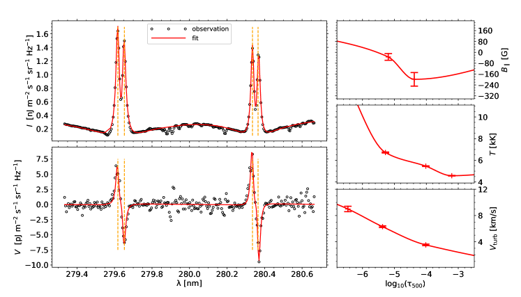
Figure 8: Same as Fig. 3, but for a pixel in the vicinity of the penumbra (yellow “$\times$” symbol in Panel (E) of Fig. 1). The vertical orange dashed lines indicate the location of the ${\rm k_{2}}$ and ${\rm h_{2}}$ peaks.

In the underlying layer at ${\rm log_{10}}(\tau_{500})=-4.5$, the inversion also shows an increase of both $T$ and $n_{\rm e}$ in the plage region underneath the moss, with respect to the quiet region. These hot regions are distributed similarly to the regions with larger magnetic flux in the photosphere (see the black and blue contours in panel (B) of Fig. 4), but covering an expanded area with respect to the latter. Inside these regions with larger photospheric magnetic flux, the inferred $n_{\rm e}$ is also larger (see the white arrows in panel (F) of Fig. 4), which suggests that the chromospheric heating is more significant inside the magnetic flux concentrations. Panel (A) of Fig. 5 shows a scatterplot between $n_{\rm e}$ at ${\rm log_{10}}(\tau_{500})=-4.5$ and the HMI longitudinal magnetic fields for the region delimited by the solid purple lines in panel (B) of Fig. 4. The correlation coefficient between both quantities is about $0.6$, which indicates the existence of some correlation, even if not a strong one. In the scatterplot, the majority of the points are located in the lower left corner (longitudinal magnetic field of 100 G or less). The reason is that, in the photosphere, most of the field of view does not show strong longitudinal magnetic field amplitudes and the inferred electron density is small in most of such areas. Besides, the region with larger electron density covers a larger area with respect to the photospheric longitudinal magnetic field, resulting in a number of points in the scatterplot with relatively large electron density but weak photospheric longitudinal magnetic field.

In Fig. 6 we show the inferred $B_{\parallel}$ at ${\rm log_{10}}(\tau_{500})=-6.0$, $-5.0$, and $-4.0$ (first, second, and third panels, from left to right, respectively). The contours in Fig. 6 are the same as in Fig. 4. The inferred $B_{\parallel}$ in the regions with photospheric flux concentrations decreases with height. The polarity of the inferred magnetic fields is consistent with that of the underlying photospheric magnetic fields. The strongest magnetic fields are found at the same location as the photospheric magnetic flux concentrations. The area occupied by the magnetic field concentrations is larger in the chromosphere than in the photosphere; these concentrations have already expanded at a height of ${\rm log_{10}}(\tau_{500})=-4.0$, almost filling up the apparently unmagnetized gaps between the flux concentrations observed in the photosphere. This is in agreement with the conclusion by Morosin et al. (2020), which posit that the magnetic canopy has formed in the lower chromosphere, where the Mg I line at 5172 Å forms. The magnetic field strengths in the chromosphere reach about $-100$ G between the photospheric flux concentrations, and about $-600$ G inside them.

The rightmost panel of Fig. 6 shows the optical depth, $\log_{10}\tau_{500}$, where $\beta=1$ (with $\beta=2\mu_{0}P_{g}/B_{\parallel}^{2}$, under the assumption that the magnetic field is parallel to the LOS, with $\mu_{0}$ the magnetic permeability). Above the regions where we find the photospheric magnetic flux concentrations, the magnetic pressure overcomes the gas pressure in the lower chromosphere. This region of the atmosphere is below the main sensitivity range of the circular polarization profile of the Mg II h and k lines.

Panels (B) and (C) of Fig. 5 show scatterplots between $B_{\parallel}$ and $n_{\rm e}$ and between $B_{\parallel}$ and $T$ at ${\rm log_{10}}(\tau_{500})=-4.5$, respectively. The correlation coefficient is about $0.8$, a correlation indicative of the magnetic origin of the heating in the plage, in agreement with the result of Ishikawa et al. (2021).

The correlation between the intensities in the moss region and the underlying chromosphere, e.g. between the 171 Å and $\rm Ly_{\alpha}$ intensities (Vourlidas et al., 2001), between the 171 Å and $\rm H_{\alpha}$ intensities (De Pontieu et al., 2003), or between the 172 Å and 2796 Å intensities (Bose et al., 2024) suggests that the heating mechanism for both the chromosphere plage and the overlying moss are closely related. The structures in the inferred magnetic field map at ${\rm log_{10}}(\tau_{500})=-6.0$ and $-4.5$ shown in Fig. 6 are morphologically similar to the outline of the moss region. Panels (D) – (G) of Fig. 5 show scatterplots between the intensity in the AIA 171 Å band and the indicated quantities resulting from the inversion. The correlation coefficients of about $0.8$ between the AIA 171 Å intensity and the (inferred) longitudinal magnetic fields at ${\rm log_{10}}(\tau_{500})=-6.0$ and $-4.5$ suggest not only a magnetic origin for the heating in the chromosphere of the plage region, but also for the heating of the moss region in the transition region.

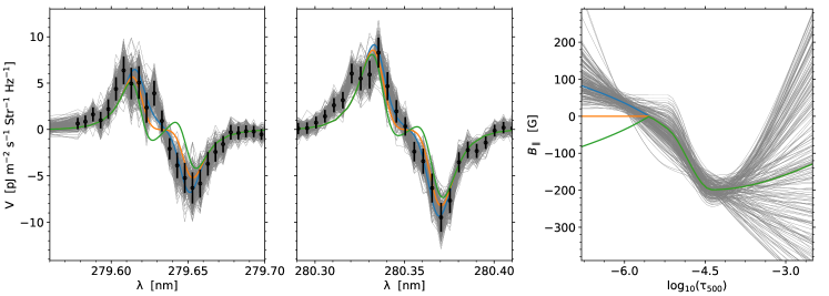
Figure 9: Two left panels: observed (open circles with error bars) and synthesized (blue, orange, and green curves) circular polarization profiles for the pixel in the vicinity of the penumbra considered in Fig. 8. Gray curves show 200 Stokes $V$ profiles generated by adding random noise to the observation. Right panel: blue (the magnetic field model from the inversion), orange (with zero magnetic fields in the upper chromosphere) and green (with flipped magnetic fields in the upper chromosphere) curves show the corresponding magnetic fields. Gray curves show the 200 Stokes $V$ profiles mentioned in the text.

4.2 The penumbra and superpenumbra

In panel (D) of Fig. 1, within the region spanning 30 – 45 arcsec in the X direction and $-50$ – 0 arcsec in Y direction, the IRIS 2796 Å slit-jaw image shows elongated fibril structures outward the penumbra, corresponding to the superpenumbra (Loughhead, 1968), which is more distinctly observed in $\rm H_{\alpha}$ and in the He I triplet lines at 10830 Å (Schad et al., 2013). This specific region is covered by slits 8 – 13 of the CLASP2.1 observation, which presents such fibrils in the intensity image at $\rm k_{2b}$ (top left panel of Fig. 2). The underlying photosphere in this region exhibits mixed polarities (see the region delimited by the dashed purple lines in panel (B) of Fig. 4). Bright features can be seen in the AIA 1600 Å band and IRIS 2796 Å slit-jaw images in these regions, while in the AIA 304 Å band there is a lack of bright features, with the exception of some bright fibrils (see Fig. 1). The inversion results show a larger temperature at ${\rm log_{10}}(\tau_{500})=-6.0$ and $-4.5$ in the superpenumbra region compared to the quiet regions, in agreement with the results of Sainz Dalda et al. (2019). In the penumbra, which occupies the region between about $-25$ – 0 arcsec for slits 15 and 16, the temperature is not significantly enhanced with respect to other regions.

At ${\rm log_{10}}(\tau_{500})=-6.0$, the inversion returns a $P_{\rm g}$ of less than 1 $\rm dyn\cdot cm^{-2}$, much lower than the average value inferred in the plage region. There is no remarkable increase in $n_{\rm e}$ either. However, some fibrils can be seen in the $n_{\rm e}$, $v_{\parallel}$, $v_{\rm turb}$, and $P_{\rm g}$ maps (see upper panels of Fig. 4).

The inferred $B_{\parallel}$ at ${\rm log_{10}}(\tau_{500})=-4.0$ shown in Fig. 6 also exhibits mixed polarities in the region between 30 – 45 arcsec in the X direction and between slits 8 – 13, and the polarity is the same as in the photosphere. The inferred $B_{\parallel}$ decreases its amplitude with height. At ${\rm log_{10}}(\tau_{500})=-6.0$, part of the negative flux disappears, for instance at around $-45$ arcsec in slits 13 and 14. As shown in Fig. 4, the regions with larger $T$ and $n_{\rm e}$ are outside the penumbra. The overall distribution of the regions with larger $T$ is similar to the distribution of the regions with larger magnetic flux. This suggests that the heating in the chromosphere of the vicinity of the sunspot is also of magnetic origin. However, when we focus on smaller scales, contrary to what was found for the plage region, the larger $n_{\rm e}$ and $T$ areas are usually located between magnetic flux concentrations (see the green arrows in panel (F) of Fig. 4). Panels (G) and (I) of Fig. 5 present scatterplots between $B_{\parallel}$ and $T$, and between $B_{\parallel}$ and $n_{\rm e}$ at ${\rm log_{10}}(\tau_{500})=-4.5$ for the region delimited by the dashed purple lines in Fig. 4. The corresponding correlation coefficients are about $-0.3$, a relatively weak negative correlation (note, however, the relatively small size of the available sample), significantly different to the correlations found for the plage region. Therefore, the details of the heating mechanisms in this region, even if the magnetic field still plays a significant role, may differ with respect to those in the plage region. It is important to emphasize that in this paper we have focused on inferring the longitudinal component of the magnetic field, so it is likely that these hot regions in between magnetic flux regions are also magnetized, but with a magnetic field which is significantly inclined with respect to the LOS.

4.3 Change of the magnetic field polarity with height

The blue, orange, and green curves in Fig. 7 show $B_{\parallel}$ at ${\rm log_{10}}(\tau_{500})=-6.0$, $-5.0$, and $-4.0$, respectively, for slits 9, 11, 15, and 16 of the CLASP2.1 observation (with the corresponding slit indicated on top of each panel). The slits locations are indicated by the blue dashed lines in Fig. 1. Slit 16 is the rightmost slit, which crosses the edge of the penumbra and the central region of some flux concentrations in the plage region.

In slit 16 (bottom right panel of Fig. 7) $B_{\parallel}$ reaches about $-600$ G at ${\rm log_{10}}(\tau_{500})=-4.0$ in the plage region, decreasing to about $-400$ G at ${\rm log_{10}}(\tau_{500})=-6.0$. At the edge of the penumbra there is an apparent lack of variation in $B_{\parallel}$.

Consistent with the weak field approximation analysis by Ishikawa et al. (2024), the inversion results also indicate changes in the polarity of the longitudinal magnetic field component $B_{\parallel}$ with height in certain areas of the slits 9, 11, and 15. For instance, such polarity changes are detected in the region between 77 and 82 arcsec in slit 9, and in the region between $-5$ and 0 arcsec in slit 11 (see Fig. 7). In Fig. 8 we show Stokes profiles corresponding to a pixel with such a polarity change. The intensity profile shows a significant reversal in the core of the Mg II h and k lines. The orange dotted lines in the figure indicate the ${\rm k_{2}}$ and ${\rm h_{2}}$ peaks. For an intensity profile with this shape, the circular polarization profile is expected to show either two pairs of lobes (see, e.g., the profile in Appendix A corresponding to the green “$\times$” symbol in Fig. 1) or almost zero inner lobes if $B_{\parallel}$ is too weak (Li et al., 2023). However, Fig. 8 shows both inner and outer lobes in circular polarization, with the same sign, thus resembling a two-lobe profile. For this to happen a polarity change from the middle to the upper chromosphere is necessary. The inversion of this profile returns a negative $B_{\parallel}$ polarity at ${\rm log_{10}}(\tau_{500})=-4.5$ (about $-200$ G) and a small, albeit positive $B_{\parallel}$ polarity, at ${\rm log_{10}}(\tau_{500})=-6.0$ (about 40 G). Since the error estimatted from the diagonal of the Hessian matrix is larger than 40 G, we carried out a Monte Carlo simulation to validate the polarity change (Westendorp Plaza et al., 2001; Sainz Dalda & De Pontieu, 2023). We generated 200 profiles by adding random Gaussian noise to the observation. The gray curves in the two left panels of Fig. 9 show the 200 Stokes $V$ profiles. We then applied the HanleRT-TIC to all profiles. Since we only use this method to investigate the uncertainty in $B_{\parallel}$, the thermodynamic parameters are fixed and only $B_{\parallel}$ is retrieved in one cycle with four nodes. The node values are randomly initialized between -500 and 500 G. The inferred $B_{\parallel}$ are shown in the right panel of Fig. 9 (see gray curves). As it was expected, all 200 inversions confirm the polarity change with height. We want to emphasize that this change in polarity was expected because it is a necessary condition for the observed shape of the circular polarization profile. To further demonstrate the need for this change of polarity, we have synthesized the circular polarization profiles for stratifications of $B_{\parallel}$ with both zero field and with no change of polarity in the upper chromosphere (see Fig. 9). As expected, if there is no polarity change the circular polarization profile shows a four-lobe shape, while the zero magnetc field shows signals very close to zero at the center of the circular polarization profile. Both syntheses fail to fit the shape of Stokes $V$ close to the line center, further confirming the polarity change.

5 Summary and conclusions

The HanleRT-TIC has been applied to the spectro-polarimetric observation of the Mg II h and k lines obtained by the CLASP2.1 suborbital space experiment. The observation, consisting of a slit scan, covers a plage region and the edge of a sunspot penumbra. We have obtained a map of the magnetic field longitudinal component in the upper chromosphere and the stratification of the thermodynamic model, including the temperature, LOS velocity, micro-turbulent velocity, and electron density and gas pressure.

In agreement with previous studies based on intensity observations of the Mg II h and k lines with IRIS, the inverted models show larger $T$ and $n_{\rm e}$ in the plage region (de la Cruz Rodríguez et al., 2016; Sainz Dalda et al., 2019). The observed plage is dominated by negative (pointing toward the solar surface) magnetic flux in both the photosphere and the middle and upper chromosphere. The inferred $B_{\parallel}$ in the chromosphere covers an area clearly expanded with respect to the magnetic field concentrations of the photospheric magnetogram, almost filling the unmagnetized gaps between the flux concentrations, which indicates that the magnetic field expands and fills the chromospheric volume below the middle chromosphere, either in the lower chromopshere (Morosin et al., 2020) or in the photosphere (Buehler et al., 2015). The pattern of the inferred $B_{\parallel}$ map overall matches the larger values of $T$ and $n_{\rm e}$ in the maps in the chromosphere, as well as the moss region in the overlying transition region seen in the AIA 171 Å band. Apart from the correlation between the intensity of the 171 Å band and $T$ and $n_{\rm e}$ (Bose et al., 2024), in this work we also show the correlation between the 171 Å intensity and $B_{\parallel}$ in the middle and upper chromosphere, which suggests the magnetic origin of the heating in both the plage and moss regions. Such correlation does not exist between the 171 Å intensity and the magnetic field inferred from the Ca II line at 854.2 nm with the WFA (Judge et al., 2024), possiblly due to the lower formation height of Ca II 854.2 nm with respect to the Mg II h and k lines. Moreover, the correlation between $B_{\parallel}$ and $T$ and $n_{\rm e}$ in the chromomosphere also suggests that heating is more significant inside the magnetic field concentrations. We also find a moderate correlation between $n_{\rm e}$ in the middle chromosphere and $B_{\parallel}$ in the photosphere, which can also be seen by visual inspection of panel (F) of Fig. 4. Such a correlation is different to that found in previous studies such as that by Anan et al. (2021), reporting no significant correlation between the magnetic field inferred from the He I triplet at 1083.0 nm and the energy flux is found.

In agreement with Sainz Dalda et al. (2019), the inferred $T$ and $n_{\rm e}$ in the superpenumbra region also show an increase with respect to the quiet regions. This increase is clearly related to the inferred magnetic field. However, their larger values are usually found between the magnetic field concentrations. The weak negative correlation between $B_{\parallel}$ and both $T$ and $n_{\rm e}$ is completely different from the correlations for the plage region. This suggests that, while the heating in this region should be of magnetic origin, the details or particularities of the heating mechanism may show differences with respect to those in the plage and moss regions. It is of interest to emphasize that in this paper we have focused on inferring only the longitudinal component of the magnetic field. Significantly inclined magnetic fields with respect to the LOS along the superpenumbral fibrils have been reported by Schad et al. (2013) from spectropolarimetric observation of the He I 1083.0 nm multiplet. Therefore, these hot regions are likely filled with more inclined magnetic fields.

Generally, we find that the inferred $B_{\parallel}$ decreases with height in the middle and upper chromomosphere. In the plage region $B_{\parallel}$ can still reach about $-400$ G in the upper chromosphere, which is consistent with the field strengths inferred from observations of the Ca II 854.2 nm line (Pietrow et al., 2020; Morosin et al., 2020; da Silva Santos et al., 2023) and the He I triplet at 1083.0 nm (Anan et al., 2021). In the penumbra, $B_{\parallel}$ does not show a significant variation with height, although there could still be some variation compatible with the uncertainties and the polarization noise. It is also noteworthy that, in agreement with the weak field approximation analysis by Ishikawa et al. (2024), our inversion results reveal changes with height in the magnetic field polarity in certain regions, namely near the penumbra and in the pore. Such a polarity change with height can be explained with a magnetic field configuration in which the magnetic field, which is anchored to the sunspot, bends down toward the photosphere at different locations for different heights, resulting in a change of polarity for a number of lines of sight.

Both, CLASP2 and CLASP2.1 measured the wavelength variation of the four Stokes parameters, but in this and in our previous paper we have focused on the inversion of the Stokes $I$ and $V$ profiles, which have allowed us to infer the longitudinal component of the magnetic field. In forthcoming papers we will consider the full Stokes-vector inversion problem of the Mg II h and k lines, showing inference results for the quiet and plage regions observed by these novel suborbital space experiments.

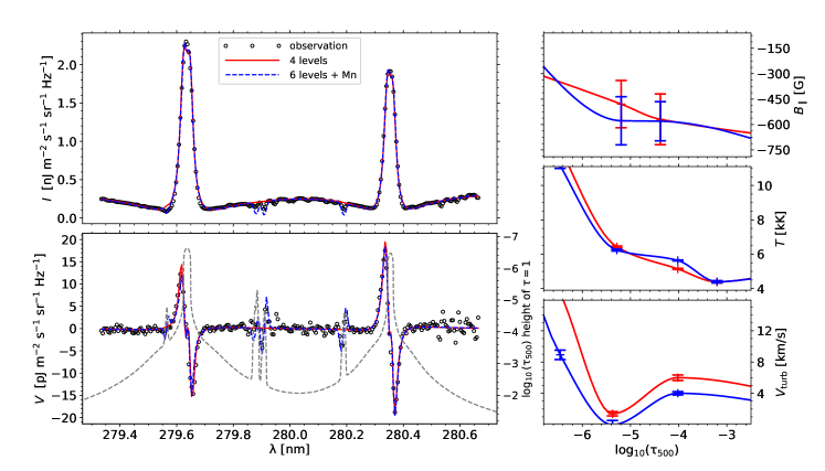
Figure 10: Same as Fig. 3 but including the inversion accounting for the Mg II UV triplet and the Mn I lines at 279.56, 279.91, and 280.19 nm. The dashed gray curve in the bottom left panel shows the optical depth (in $\rm log_{10}(\tau_{500})$) corresponding to the atmosphere height for which the optical depth at any given wavelength is equal to one ($\tau_{\lambda}=1$).

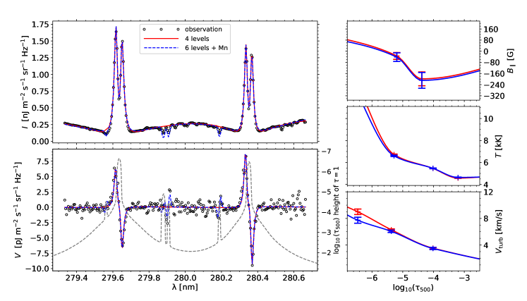
Figure 11: Same as Fig. 10 but for a pixel in the vicinity of the penumbra (yellow “$\times$” symbol in Panel (E) of Fig. 1). The red solid curve is the same as in Fig. 8.

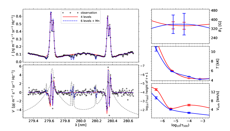
Figure 12: Same as Fig. 10, but for a pixel in the penumbra (green “$\times$” symbol in Panel (E) of Fig. 1).

Appendix A The impact of the Mn I lines and the Mg II subordinate lines on the inferred model

In the spectral region observed by the CLASP2.1 there are three resonance lines of Mn I at 279.56, 279.91, and 280.19 nm, as well as two blended lines of Mg II at 279.88 nm. These lines form in the lower chromosphere (Pereira et al., 2015; del Pino Alemán et al., 2020, 2022). Here we investigate the impact of including these lines in the inversion. Even though accounting for HFS is necessary to correctly model the Mn I lines, its general treatment is not included in our inversion code. Consequently, we neglect HFS in the inversion. Neglecting the HFS affects the width of the lines and leads to an underestimation of the circular polarization signal (del Pino Alemán et al., 2022). Moreover, their accurate modeling requires an atomic model with a large number of levels and transitions. Due to these reasons, our modeling of the Mn I profiles is very approximate. Nevertheless, including the Mn I lines and the Mg II UV triplet lines while giving more weight in the inversion to the Mg II h and k lines, can add additional information in the lower chromosphere region without significantly impacting the fitting to the Mg II h and k lines. To include the UV triplet lines we add their two upper levels to the Mg model described in Sec. 3. The Mn atomic model has nine levels, four Mn I levels, four Mn II levels, and the ground level of Mn III.

In Figs. 10–12 we show the result of the inversion (following the strategy described in Sec. 3) for a pixel in the plage, for a pixel in the vicinity of the penumbra, and for a pixel in the penumbra (red, yellow, and green “$\times$” symbols in panel (E) of Fig. 1), respectively. The dashed gray curve in the bottom left panel of the figures show the optical depth (in $\rm log_{10}(\tau_{500})$) where the optical depth at each wavelength is equal to one ($\tau_{\lambda}=1$), which roughly indicates the formation regions of the Mg II and Mn I lines: the inner lobes of the circular polarization profiles of the h and k lines form at around ${\rm log_{10}}(\tau_{500})=-6.0$ (upper chromosphere), while their outer lobes form between around ${\rm log_{10}}(\tau_{500})=-4.0$ and $-5.0$ (middle chromosphere); the lobes of the circular polarization profiles of the Mn I lines and the Mg II subordinate lines form deeper in the atmosphere (lower chromosphere). The inferred $B_{\parallel}$, $T$, and $v_{\rm turb}$ are shown in the right column of the figure. In Fig. 11, the two inversions return very similar results, compatible within the error bars (see Sec. 3). The fitting of the Stokes profiles of the Mn I lines, and the Mg II UV triplet lines are not as good as for the h and k lines. Even though the fit could be improved by adding more weight them, or by adding more nodes in their region of formation, the approximations in the modeling of the Mn I lines would lead to a worse fit of the h and k lines, and thus, additional inaccuracies in the inferred model.

For the inversion in Figs. 10 and 12 the differences between the two approaches are more significant, especially for $v_{\rm turb}$. Although we think that the inversion including the Mn I lines and the Mg II UV triplet lines (red curves in Figs. 10 – 12) is more reliable, since the these lines can add better constraints to the model in the lower chromosphere and especially the Mg II lines at 279.88 nm are sensitive to the temperature increase at the temperature minimum region (Pereira et al., 2015), the inversion results with only 4 Mg levels are also acceptable, with both solutions of $B_{\parallel}$ usually being fully compatible within the error bars. Therefore, in order to reduce the already significant computing time, we perform the inversion of only the h and k lines at all the pixels with the four level Mg model. On average, the inversion still takes around 10 CPU hours for each pixel. Besides, we have set an upper limit of 6 km s^-1 to the micro-turbulent velocity at ${\rm log_{10}}(\tau_{500})=-4.0$ to avoid a compatible large value, because the micro-turbulent velocity is typically found to be smaller than 6 km s^-1 at those heights (Sainz Dalda et al., 2019).

References

- Alsina Ballester et al. (2016) Alsina Ballester, E., Belluzzi, L., & Trujillo Bueno, J. 2016, ApJ, 831, L15, doi: 10.3847/2041-8205/831/2/L15
- Anan et al. (2021) Anan, T., Schad, T. A., Kitai, R., et al. 2021, ApJ, 921, 39, doi: 10.3847/1538-4357/ac1b9c
- Asensio Ramos et al. (2007) Asensio Ramos, A., Martínez González, M. J., & Rubiño-Martín, J. A. 2007, A&A, 476, 959, doi: 10.1051/0004-6361:20078107
- Belluzzi & Trujillo Bueno (2012) Belluzzi, L., & Trujillo Bueno, J. 2012, ApJ, 750, L11, doi: 10.1088/2041-8205/750/1/L11
- Belluzzi & Trujillo Bueno (2014) —. 2014, A&A, 564, A16, doi: 10.1051/0004-6361/201321598
- Belluzzi et al. (2012) Belluzzi, L., Trujillo Bueno, J., & Štěpán, J. 2012, ApJ, 755, L2, doi: 10.1088/2041-8205/755/1/L2
- Berger et al. (1999) Berger, T. E., De Pontieu, B., Fletcher, L., et al. 1999, Sol. Phys., 190, 409, doi: 10.1023/A:1005286503963
- Bose et al. (2024) Bose, S., De Pontieu, B., Hansteen, V., et al. 2024, Nature Astronomy, doi: 10.1038/s41550-024-02241-8
- Buehler et al. (2015) Buehler, D., Lagg, A., Solanki, S. K., & van Noort, M. 2015, A&A, 576, A27, doi: 10.1051/0004-6361/201424970
- Carlsson et al. (2019) Carlsson, M., De Pontieu, B., & Hansteen, V. H. 2019, ARA&A, 57, 189, doi: 10.1146/annurev-astro-081817-052044
- Carlsson et al. (2015) Carlsson, M., Leenaarts, J., & De Pontieu, B. 2015, ApJ, 809, L30, doi: 10.1088/2041-8205/809/2/L30
- Casini et al. (2017a) Casini, R., del Pino Alemán, T., & Manso Sainz, R. 2017a, ApJ, 835, 114, doi: 10.3847/1538-4357/835/2/114
- Casini et al. (2017b) —. 2017b, ApJ, 848, 99, doi: 10.3847/1538-4357/aa8a73
- Casini et al. (2014) Casini, R., Landi Degl’Innocenti, M., Manso Sainz, R., Land i Degl’Innocenti, E., & Landolfi, M. 2014, ApJ, 791, 94, doi: 10.1088/0004-637X/791/2/94
- da Silva Santos et al. (2023) da Silva Santos, J. M., Reardon, K., Cauzzi, G., et al. 2023, ApJ, 954, L35, doi: 10.3847/2041-8213/acf21f
- de la Cruz Rodríguez et al. (2016) de la Cruz Rodríguez, J., Leenaarts, J., & Asensio Ramos, A. 2016, ApJ, 830, L30, doi: 10.3847/2041-8205/830/2/L30
- de la Cruz Rodríguez & van Noort (2017) de la Cruz Rodríguez, J., & van Noort, M. 2017, Space Sci. Rev., 210, 109, doi: 10.1007/s11214-016-0294-8
- De Pontieu et al. (2003) De Pontieu, B., Tarbell, T., & Erdélyi, R. 2003, ApJ, 590, 502, doi: 10.1086/374928
- De Pontieu et al. (2014) De Pontieu, B., Title, A. M., Lemen, J. R., et al. 2014, Sol. Phys., 289, 2733, doi: 10.1007/s11207-014-0485-y
- del Pino Alemán et al. (2022) del Pino Alemán, T., Alsina Ballester, E., & Trujillo Bueno, J. 2022, ApJ, 940, 78, doi: 10.3847/1538-4357/ac922c
- del Pino Alemán et al. (2016) del Pino Alemán, T., Casini, R., & Manso Sainz, R. 2016, ApJ, 830, L24, doi: 10.3847/2041-8205/830/2/L24
- del Pino Alemán et al. (2020) del Pino Alemán, T., Trujillo Bueno, J., Casini, R., & Manso Sainz, R. 2020, ApJ, 891, 91, doi: 10.3847/1538-4357/ab6bc9
- del Toro Iniesta (2003) del Toro Iniesta, J. C. 2003, Introduction to Spectropolarimetry
- del Toro Iniesta & Ruiz Cobo (2016) del Toro Iniesta, J. C., & Ruiz Cobo, B. 2016, Living Reviews in Solar Physics, 13, 4, doi: 10.1007/s41116-016-0005-2
- Fletcher & De Pontieu (1999) Fletcher, L., & De Pontieu, B. 1999, ApJ, 520, L135, doi: 10.1086/312157
- Ishikawa et al. (2024) Ishikawa, R., Trujillo Bueno, J., McKenzie, D., & et al. 2024, in preparation
- Ishikawa et al. (2021) Ishikawa, R., Trujillo Bueno, J., del Pino Alemán, T., et al. 2021, Science Advances, 7, eabe8406, doi: 10.1126/sciadv.abe8406
- Ishikawa et al. (2023) Ishikawa, R., Trujillo Bueno, J., Alsina Ballester, E., et al. 2023, ApJ, 945, 125, doi: 10.3847/1538-4357/acb64e
- Judge et al. (2022) Judge, P., Bryans, P., Casini, R., et al. 2022, ApJ, 941, 159, doi: 10.3847/1538-4357/aca2a5
- Judge et al. (2024) Judge, P., Kleint, L., Casini, R., et al. 2024, ApJ, 960, 129, doi: 10.3847/1538-4357/ad0780
- Kano et al. (2012) Kano, R., Bando, T., Narukage, N., et al. 2012, in Society of Photo-Optical Instrumentation Engineers (SPIE) Conference Series, Vol. 8443, Space Telescopes and Instrumentation 2012: Ultraviolet to Gamma Ray, ed. T. Takahashi, S. S. Murray, & J.-W. A. den Herder, 84434F, doi: 10.1117/12.925991
- Kano et al. (2017) Kano, R., Trujillo Bueno, J., Winebarger, A., et al. 2017, ApJ, 839, L10, doi: 10.3847/2041-8213/aa697f
- Kobayashi et al. (2012) Kobayashi, K., Kano, R., Trujillo-Bueno, J., et al. 2012, in Astronomical Society of the Pacific Conference Series, Vol. 456, Fifth Hinode Science Meeting, ed. L. Golub, I. De Moortel, & T. Shimizu, 233
- Lagg et al. (2017) Lagg, A., Lites, B., Harvey, J., Gosain, S., & Centeno, R. 2017, Space Sci. Rev., 210, 37, doi: 10.1007/s11214-015-0219-y
- Leenaarts et al. (2012) Leenaarts, J., Pereira, T., & Uitenbroek, H. 2012, A&A, 543, A109, doi: 10.1051/0004-6361/201219394
- Lemen et al. (2012) Lemen, J. R., Title, A. M., Akin, D. J., et al. 2012, Sol. Phys., 275, 17, doi: 10.1007/s11207-011-9776-8
- Li et al. (2022) Li, H., del Pino Alemán, T., Trujillo Bueno, J., & Casini, R. 2022, ApJ, 933, 145, doi: 10.3847/1538-4357/ac745c
- Li et al. (2019) Li, H., Xu, Z., Qu, Z., & Sun, L. 2019, ApJ, 875, 127, doi: 10.3847/1538-4357/ab0f35
- Li et al. (2023) Li, H., del Pino Alemán, T., Trujillo Bueno, J., et al. 2023, ApJ, 945, 144, doi: 10.3847/1538-4357/acb76e
- Loughhead (1968) Loughhead, R. E. 1968, Sol. Phys., 5, 489, doi: 10.1007/BF00147015
- Martens et al. (2000) Martens, P. C. H., Kankelborg, C. C., & Berger, T. E. 2000, ApJ, 537, 471, doi: 10.1086/309000
- Mihalas (1978) Mihalas, D. 1978, Stellar atmospheres (SanFrancisco:Freeman)
- Milić & van Noort (2018) Milić, I., & van Noort, M. 2018, A&A, 617, A24, doi: 10.1051/0004-6361/201833382
- Morosin et al. (2020) Morosin, R., de la Cruz Rodríguez, J., Vissers, G. J. M., & Yadav, R. 2020, A&A, 642, A210, doi: 10.1051/0004-6361/202038754
- Narukage et al. (2016) Narukage, N., McKenzie, D. E., Ishikawa, R., et al. 2016, in Society of Photo-Optical Instrumentation Engineers (SPIE) Conference Series, Vol. 9905, Space Telescopes and Instrumentation 2016: Ultraviolet to Gamma Ray, ed. J.-W. A. den Herder, T. Takahashi, & M. Bautz, 990508, doi: 10.1117/12.2232245
- Pereira et al. (2015) Pereira, T. M. D., Carlsson, M., De Pontieu, B., & Hansteen, V. 2015, ApJ, 806, 14, doi: 10.1088/0004-637X/806/1/14
- Pesnell et al. (2012) Pesnell, W. D., Thompson, B. J., & Chamberlin, P. C. 2012, Sol. Phys., 275, 3, doi: 10.1007/s11207-011-9841-3
- Pietrow et al. (2020) Pietrow, A. G. M., Kiselman, D., de la Cruz Rodríguez, J., et al. 2020, A&A, 644, A43, doi: 10.1051/0004-6361/202038750
- Rachmeler et al. (2022) Rachmeler, L. A., Trujillo Bueno, J., McKenzie, D. E., et al. 2022, ApJ, 936, 67, doi: 10.3847/1538-4357/ac83b8
- Sainz Dalda et al. (2019) Sainz Dalda, A., de la Cruz Rodríguez, J., De Pontieu, B., & Gošić, M. 2019, ApJ, 875, L18, doi: 10.3847/2041-8213/ab15d9
- Sainz Dalda & De Pontieu (2023) Sainz Dalda, A., & De Pontieu, B. 2023, ApJ, 944, 118, doi: 10.3847/1538-4357/acb2c7
- Schad et al. (2013) Schad, T. A., Penn, M. J., & Lin, H. 2013, ApJ, 768, 111, doi: 10.1088/0004-637X/768/2/111
- Schou et al. (2012) Schou, J., Scherrer, P. H., Bush, R. I., et al. 2012, Sol. Phys., 275, 229, doi: 10.1007/s11207-011-9842-2
- Song et al. (2018) Song, D., Ishikawa, R., Kano, R., et al. 2018, in Society of Photo-Optical Instrumentation Engineers (SPIE) Conference Series, Vol. 10699, Space Telescopes and Instrumentation 2018: Ultraviolet to Gamma Ray, ed. J.-W. A. den Herder, S. Nikzad, & K. Nakazawa, 106992W, doi: 10.1117/12.2313056
- Trujillo Bueno & del Pino Alemán (2022) Trujillo Bueno, J., & del Pino Alemán, T. 2022, ARA&A, 60, 415, doi: 10.1146/annurev-astro-041122-031043
- Trujillo Bueno et al. (2017) Trujillo Bueno, J., Landi Degl’Innocenti, E., & Belluzzi, L. 2017, Space Sci. Rev., 210, 183, doi: 10.1007/s11214-016-0306-8
- Trujillo Bueno et al. (2012) Trujillo Bueno, J., Štěpán, J., & Belluzzi, L. 2012, ApJ, 746, L9, doi: 10.1088/2041-8205/746/1/L9
- Trujillo Bueno et al. (2011) Trujillo Bueno, J., Štěpán, J., & Casini, R. 2011, ApJ, 738, L11, doi: 10.1088/2041-8205/738/1/L11
- Trujillo Bueno et al. (2018) Trujillo Bueno, J., Štěpán, J., Belluzzi, L., et al. 2018, ApJ, 866, L15, doi: 10.3847/2041-8213/aae25a
- Tsuzuki et al. (2020) Tsuzuki, T., Ishikawa, R., Kano, R., et al. 2020, in Society of Photo-Optical Instrumentation Engineers (SPIE) Conference Series, Vol. 11444, Society of Photo-Optical Instrumentation Engineers (SPIE) Conference Series, 114446W, doi: 10.1117/12.2562273
- Vourlidas et al. (2001) Vourlidas, A., Klimchuk, J. A., Korendyke, C. M., Tarbell, T. D., & Handy, B. N. 2001, ApJ, 563, 374, doi: 10.1086/323835
- Štěpán et al. (2015) Štěpán, J., Trujillo Bueno, J., Leenaarts, J., & Carlsson, M. 2015, ApJ, 803, 65, doi: 10.1088/0004-637X/803/2/65
- Westendorp Plaza et al. (2001) Westendorp Plaza, C., del Toro Iniesta, J. C., Ruiz Cobo, B., et al. 2001, ApJ, 547, 1130, doi: 10.1086/318376
- Wittmann (1974) Wittmann, A. 1974, Sol. Phys., 35, 11, doi: 10.1007/BF00156952