Approximating Discrimination Within Models When Faced With Several Non-Binary Sensitive Attributes

Abstract

Discrimination mitigation with machine learning (ML) models could be complicated because multiple factors may interweave with each other including hierarchically and historically. Yet few existing fairness measures are able to capture the discrimination level within ML models in the face of multiple sensitive attributes. To bridge this gap, we propose a fairness measure based on distances between sets from a manifold perspective, named as ‘harmonic fairness measure via manifolds (HFM)’ with two optional versions, which can deal with a fine-grained discrimination evaluation for several sensitive attributes of multiple values. To accelerate the computation of distances of sets, we further propose two approximation algorithms named ‘Approximation of distance between sets for one sensitive attribute with multiple values (ApproxDist)’ and ‘Approximation of extended distance between sets for several sensitive attributes with multiple values (ExtendDist)’ to respectively resolve bias evaluation of one single sensitive attribute with multiple values and that of several sensitive attributes with multiple values. Moreover, we provide an algorithmic effectiveness analysis for ApproxDist under certain assumptions to explain how well it could work. The empirical results demonstrate that our proposed fairness measure HFM is valid and approximation algorithms (i.e., ApproxDist and ExtendDist) are effective and efficient.

1 Introduction

As techniques of machine learning (ML) and deep learning (DL) are flourishing developed and ML/DL systems are widely deployed in real life nowadays, the concern about the underlying discrimination hidden in these models has grown, particularly in high-stakes domains such as healthcare, recruitment, and jurisdiction [1], where equity for all stakeholders is pivotal to prevent unjust outcomes, akin to a discriminatory Matthew Effect. It is of significance to prevent ML models from perpetuating or exacerbating inappropriate human prejudices for not only model performance but also societal welfare. Effectively addressing and eliminating discrimination usually requires a comprehensive grasp of its occurrence, causes, and mechanisms. For instance, a case involving a person changing their gender for lower car insurance rates highlights the complexity of fairness in ML.

Although the impressive practical advancements of ML and DL thrive on abundant data, their trustworthiness and equity heavily hinge on data quality. In fact, one of the primary sources of unfairness identified in the existing literature is biases from the data, possibly collected from various sources such as device measurements and historically biassed human decisions [2]. Moreover, the challenge of data imbalance often looms in human-sensitive domains, amplifying concerns of discrimination and bias propagation in ML models. Then misformed model training would amplify imbalances and biases in data, with wide-reaching societal implications. For example, optimising aggregated prediction errors can advantage privileged groups over marginalised ones. In addition, missing data like instances or values may introduce disparities between the dataset and the target population, leading to biassed results as well. Therefore, in order to ensure fairness and mitigate biases, it is crucial to correctly cope with data imbalance and prevent ML models from perpetuating or even exacerbating inappropriate human prejudices.

To mitigate bias within ML models, the very first step to promptly recognise its occurrence. However, promptly detecting discrimination fully, truly, and faithfully is not quite easy because of plenty of factors interweaving with each other. First, learning algorithms might yield unfair outcomes even with purely clean data due to proxy attributes for sensitive features or tendentious algorithmic objectives. For instance, the educational background of one person might be a proxy attribute for those born in families with a preference for boys. Second, the existence of multiple sensitive attributes and their twist with each other highlight the complexity of bias tackling, like one member from a marginalised group could become one of the majority concerning another factor, or vice versa. Third, dynamic changes and historical factors may need to be taken into account, as bias hidden in data, data imbalance, and present decisions may interweave, causing some interrelated impact and vicious circles. Despite many fairness measures that have been proposed to facilitate bias mitigation, most of them mainly focus on one single sensitive attribute or ones with binary values, and few could handle bias appropriately when facing multiple sensitive attributes with even multiple values. Therefore, it motivates us to investigate a proper tool to deal with bias in such aforementioned scenarios.

In this paper, we investigate the possibility of assessing the discrimination level of ML models in the existence of several sensitive attributes with multiple values. To this end, we introduce a novel fairness measure from a manifold perspective, named ‘harmonic fairness measure via manifolds (HFM)’, with two optional versions (that is, maximum HFM and average HFM). However, the direct calculation of HFM lies on a core distance between two sets, which might be pretty costly. Therefore, we further propose two approximation algorithms that quickly estimate the distance between sets, named as ‘Approximation of distance between sets for one sensitive attribute with multiple values (ApproxDist)’ and ‘Approximation of extended distance between sets for several sensitive attributes with multiple values (ExtendDist)’ respectively, in order to speed up the calculation and enlarge its practical applicable values. Furthermore, we also investigate their algorithmic properties under certain reasonable assumptions, in other words, how effective they could be in achieving the approximation goal. Our contribution in this work is four-fold:

• We propose a fairness measure named HFM that could reflect the discrimination level of classifiers even simultaneously facing several sensitive attributes with multiple values. Note that HFM has two optional versions, of which both are built on a concept of distances between sets from the manifold perspective.

• We propose two approximation algorithms (that is, ApproxDist and ExtendDist) that accelerate the estimation of distances between sets, to mitigate its disadvantage of costly direct calculation of HFM.

• We further investigate the algorithmic effectiveness of ApproxDist and ExtendDist under certain assumptions and provide detailed explanations.

• Comprehensive experiments are conducted to demonstrate the effectiveness of the proposed HFM and approximation algorithms.

2 Related Work

In this section, we firstly introduce existing techniques to enhance fairness and then summarise available metrics to measure fairness for ML models in turn.

2.1 Techniques to enhance fairness

Existing mechanisms to mitigate biases and enhance fairness in ML models could be typically divided into three types: pre-processing, in-processing, and post-processing mechanisms, based on when manipulations are applied during model training pipelines. Particularly, recent work on in-processing fairness for DL models mainly falls under two types of approaches: constraint-based and adversarial learning methods [3]. Constraint-based methods usually incorporate fairness metrics directly into the model optimisation objectives as constraints or regularisation terms. For instance, Zemel et al. [4], the pioneer in this direction, put demographic parity constraints on model predictions. Subsequent work also includes using approximations [5] or modified training schemes [6] to improve scalability. Adversarial methods intend to learn representations as fairly as possible by removing sensitive attribute information. In such procedures, additional prediction heads may be introduced for attribute subgroup predictions and the information concerning sensitive attributes would be removed through inverse gradient updating [7, 8] or disentangling features [9, 10, 11, 12]. Other fairness enhancing techniques include data augmentations [13], sampling [14, 15], data noising [16], dataset balancing with generative methods [17, 18, 19], and reweighting mechanisms [20, 21]. Recently, mixup operations [22, 23, 3] are adopted to enhance fairness by blending inputs across subgroups [24, 25]. However, most of these studies focus on protecting one single sensitive attribute and are hardly able to deal with several sensitive attributes all at once. And multi-attribute fairness protection remains relatively rarely explored.

2.2 Existing fairness metrics and multi-attribute fairness protection

The well-known fairness metrics are generally divided into group fairness—such as demographic parity (DP), equality of opportunity (EO), and predictive quality parity (PQP)—and individual fairness [26, 27, 28, 29, 30]. The former mainly focuses on statistical/demographic equality among groups defined by sensitive attributes, while the latter cares more about the principle that ‘similar individuals should be evaluated or treated similarly.’ However, satisfying fairness metrics all at once is hard to achieve because they are usually not compatible with each other [31]. In practice, it may need to deliberate on the choice of the specified distance in individual fairness [29, 26]. Moreover, the three commonly used group fairness measures (that is, DP, EO, and PQP) can only deal with one single sensitive attribute with binary values. Although extending them to scenarios of one sensitive attribute with multiple values is possible, they are still limited when facing several sensitive attributes at the same time. Recent work includes a newly proposed fairness measure named discriminative risk (DR) [32] that is capable of capturing bias from both individual and group fairness aspects and two fairness frameworks (that is, InfoFair [33] and MultiFair [3]) to deliver fair predictions in face of multiple sensitive attributes. Yet these two fairness frameworks are not measures that could directly evaluate the discrimination level of ML models.

3 Methodology

In this section, we formally study the measurement of fairness from a manifold perspective. Here is a list of some standard notations we use. In this paper, we denote the scalars by italic lowercase letters (e.g., $x$), the vectors by bold lowercase letters (e.g., $\bm{x}$), the matrices/sets by italic uppercase letters (e.g., $X$), the random variables by serif uppercase letters (e.g., $\mathsf{X}$), the real numbers (resp. the integers, and the positive integers) by $\mathbb{R}$ (resp. $\mathbb{Z}$, and $\mathbb{Z}_{+}$), the probability measure (resp. the expectation, and the variance of one random variable) by $\mathbb{P}(\cdot)$ (resp. $\mathbb{E}(\cdot)$ and $\mathbb{V}(\cdot)$), the indicator function by $\mathbb{I}(\cdot)$, and the hypothesis space (resp. models in it) by $\mathcal{F}$ (resp. $f(\cdot)$).

In this paper, $i\in[n]$ is used to represent $i\in\{1,2,...,n\}$ for brevity. We use $S=\{(\bm{x}_{i},y_{i})\}_{i=1}^{n}$ to denote a dataset where the instances are iid. (independent and identically distributed), drawn from an feature-label space $\mathcal{X\!\times\!Y}$ based on an unknown distribution. The feature/input space $\mathcal{X}$ is arbitrary, and the label/output space $\mathcal{Y}\!=\!\{1,2,...,n_{c}\}(n_{c}\geqslant 2)$ is finite, which could be binary or multi-class classification, depending on the number of labels (i.e., the value of $n_{c}$). Presuming that the considered dataset $S$ is composed of the instances including sensitive attributes, the features of one instance including sensitive attributes $\bm{a}\!=\![a_{1},a_{2},...,a_{n_{a}}]^{\mathsf{T}}$ is represented as $\bm{x}\triangleq(\mathop{\breve{\bm{x}}},\mathop{\bm{a}})$, where $n_{a}\geqslant 1$ is the number of sensitive attributes allowing multiple attributes and $a_{i}\!\in\!\mathbb{Z}_{+}(1\!\leqslant\!i\!\leqslant\!n_{a})$ allows both binary and multiple values. A function $f\!\in\!\mathcal{F}:\mathcal{X\!\mapsto\!Y}$ represents a hypothesis in a space of hypotheses $\mathcal{F}$, of which the prediction for one instance $\bm{x}$ is denoted by $f(\bm{x})$ or $\hat{y}$.

3.1 Model fairness assessment from a manifold perspective

Given the dataset $S\!=\!\{(\mathop{\breve{\bm{x}}}_{i},\mathop{\bm{a}}_{i},y_{i})|i\in[n]\}$ composed of instances including sensitive attributes, here we denote one instance by $\bm{x}=(\mathop{\breve{\bm{x}}},\mathop{\bm{a}})=[x_{1},...,x_{n_{x}},a_{1},...,a_{n_{a}}]^{\mathsf{T}}$ for clarity, where $n_{a}$ is the number of sensitive/protected attributes and $n_{x}$ is that of unprotected attributes in $\bm{x}$. In this paper, we introduce new fairness measures in scenarios for multiple sensitive attributes with multiple possible values. Note that the proposed fairness measure in this paper is extended from our previous work—a fairness measure in scenarios for sensitive attributes with binary values [34].

3.1.1 Distance between sets for sensitive attributes with binary values, from our previous work [34]

Inspired by the principle of individual fairness—similar treatment for similar individuals, if we view the instances (with the same sensitive attributes) as data points on certain manifolds, the manifold representing members from the marginalised/unprivileged group(s) is supposed to be as close as possible to that representing members from the privileged group. To measure the fairness with respect to the sensitive attribute, we have proposed a fairness measure that is inspired by ‘the distance of sets’ introduced in mathematics. For a certain bi-valued sensitive attribute $a_{i}\!\in\!\mathcal{A}_{i}\!=\!\{0,1\}$, $S$ can be divided into two subsets $S_{1}\!=\!\{(\bm{x},y)\!\in S|a_{i}\!=\!1\}$ and $\bar{S}_{1}\!=\!S\setminus S_{1}\!=\!\{(\bm{x},y)\!\in S|a_{i}\!\neq\!1\}$, where $a_{i}\!=\!1$ means the corresponding instance is a member from the privileged group. Then given a specific distance metric $\mathbf{d}(\cdot,\cdot)$ on the feature space, our previous distance between these two subsets (that is, $S_{1}$ and $\bar{S}_{1}$) is defined by

$$\small\begin{split}\mathbf{D}(S_{1},\bar{S}_{1})\triangleq\max\big{\{}&\max_{(\bm{x},y)\in S_{1}}\min_{(\bm{x}^{\prime},y^{\prime})\in\bar{S}_{1}}\mathbf{d}\big{(}(\mathop{\breve{\bm{x}}},y),({\mathop{\breve{\bm{x}}}}^{\prime},y^{\prime})\big{)},\\ &\max_{(\bm{x}^{\prime},y^{\prime})\in\bar{S}_{1}}\min_{(\bm{x},y)\in S_{1}}\mathbf{d}\big{(}(\mathop{\breve{\bm{x}}},y),({\mathop{\breve{\bm{x}}}}^{\prime},y^{\prime})\big{)}\big{\}}\,,\end{split}$$ (1)

and it is viewed as the distance between the manifolds of marginalised group(s) and that of the privileged group. Notice that this distance satisfies three basic properties: identity, symmetry, and triangle inequality. Analogously, for a trained classifier $f(\cdot)$, we can calculate

$$\small\begin{split}\mathbf{D}_{f}(S_{1},\bar{S}_{1})=\max\big{\{}&\max_{(\bm{x},y)\in S_{1}}\min_{(\bm{x}^{\prime},y^{\prime})\in\bar{S}_{1}}\mathbf{d}\big{(}(\mathop{\breve{\bm{x}}},\hat{y}),({\mathop{\breve{\bm{x}}}}^{\prime},\hat{y}^{\prime})\big{)},\\ &\max_{(\bm{x}^{\prime},y^{\prime})\in\bar{S}_{1}}\min_{(\bm{x},y)\in S_{1}}\mathbf{d}\big{(}(\mathop{\breve{\bm{x}}},\hat{y}),({\mathop{\breve{\bm{x}}}}^{\prime},\hat{y}^{\prime})\big{)}\big{\}}\,.\end{split}$$ (2)

By recording the true label $y$ and the prediction $\hat{y}$ as one denotation (say $\ddot{y}$) for simplification, we could rewrite Equations (1) and (2) as

$$\small\begin{split}\mathbf{D}_{\cdot}(S_{1},\bar{S}_{1})\triangleq\max\big{\{}&\max_{(\bm{x},y)\in S_{1}}\min_{(\bm{x}^{\prime},y^{\prime})\in\bar{S}_{1}}\mathbf{d}\big{(}(\breve{\bm{x}},{\ddot{y}}),(\breve{\bm{x}}^{\prime},{\ddot{y}}^{\prime})\big{)},\\ &\max_{(\bm{x}^{\prime},y^{\prime})\in\bar{S}_{1}}\min_{(\bm{x},y)\in S_{1}}\mathbf{d}\big{(}(\breve{\bm{x}},{\ddot{y}}),(\breve{\bm{x}}^{\prime},{\ddot{y}}^{\prime})\big{)}\big{\}}\,.\end{split}$$ (3)

We will continue using the above notations in the subsequent context for simplification.

3.1.2 Distance between sets for one sensitive attribute with multiple values

As for the scenarios where only one sensitive attribute exists, let $\mathop{\bm{a}}=[a_{i}]^{\mathsf{T}}$ be a single sensitive attribute, in other words, $n_{a}\!=\!1$, $a_{i}\!\in\!\mathcal{A}_{i}\!=\!\{1,2,...,n_{a_{i}}\}$, $n_{a_{i}}\!\geqslant 3$, and $n_{a_{i}}\!\in\!\mathbb{Z}_{+}$. Then the original dataset $S$ can be divided into a few disjoint sets according to the value of this attribute $a_{i}$, that is, $S_{j}=\{(\bm{x},y)\in S\mid a_{i}=j\},\forall j\in\mathcal{A}_{i}$. We can now extend Eq. (3) and introduce the following distance measures: (i) maximal distance measure for one sensitive attribute

$$\small\mathbf{D}_{\cdot,\bm{a}}^{\text{}}(S,a_{i})\triangleq\max_{1\leqslant j\leqslant n_{a_{i}}}\big{\{}\max_{(\bm{x},y)\in S_{j}}\min_{(\bm{x}^{\prime},y^{\prime})\in\bar{S}_{j}}\mathbf{d}\big{(}(\breve{\bm{x}},{\ddot{y}}),(\breve{\bm{x}}^{\prime},{\ddot{y}}^{\prime})\big{)}\big{\}}\,,$$ (4)

and (ii) average distance measure for one sensitive attribute

$$\small\mathbf{D}_{\cdot,\bm{a}}^{\text{avg}}(S,a_{i})\triangleq\frac{1}{n}\sum_{j=1}^{n_{a_{i}}}\sum_{(\bm{x},y)\in S_{j}}\min_{(\bm{x}^{\prime},y^{\prime})\in\bar{S}_{j}}\mathbf{d}\big{(}(\breve{\bm{x}},{\ddot{y}}),(\breve{\bm{x}}^{\prime},{\ddot{y}}^{\prime})\big{)}\,,$$ (5)

where $\bar{S}_{j}\!=S\!\setminus\!S_{j}$. Notice that $\mathbf{D}_{\cdot,\bm{a}}^{\text{}}(S,a_{i})\!=\!\mathbf{D}_{\cdot}(S_{1},\bar{S}_{1})$ when $\mathcal{A}_{i}\!=\!\{0,1\}$.

3.1.3 Distance between sets for multiple sensitive attributes with multiple values

Now we discuss the general case, where we have several sensitive attributes $\mathop{\bm{a}}=[a_{1},a_{2},...,a_{n_{a}}]^{\mathsf{T}}$ and each $a_{i}\in\mathcal{A}_{i}=\{1,2,..,n_{a_{i}}\}$, where $n_{a_{i}}$ is the number of values for this sensitive attribute $a_{i}\,(1\leqslant i\leqslant n_{a})$. We can now introduce the following generalised distance measures: (i) maximal distance measure for sensitive attributes

$$\small\mathbf{D}_{\cdot,\bm{a}}^{\text{}}(S)\triangleq\max_{1\leqslant i\leqslant n_{a}}\mathbf{D}_{\cdot,\bm{a}}^{\text{}}(S,a_{i})\,,$$ (6)

and (ii) average distance measure for sensitive attributes

$$\small\mathbf{D}_{\cdot,\bm{a}}^{\text{avg}}(S)\triangleq\frac{1}{n_{a}}\sum_{i=1}^{n_{a}}\mathbf{D}_{\cdot,\bm{a}}^{\text{avg}}(S,a_{i})\,.$$ (7)

Remark.

1. It is easy to see that $\mathbf{D}_{\cdot,\bm{a}}^{\text{}}(S)\geqslant\mathbf{D}_{\cdot,\bm{a}}^{\text{avg}}(S)$.

2. Both $\mathbf{D}_{\cdot,\bm{a}}^{\text{}}(S,a_{i})$ and $\mathbf{D}_{\cdot,\bm{a}}^{\text{avg}}(S,a_{i})$ measure the fairness regarding the sensitive attribute $a_{i}$.

3. As their names suggest, the maximal distance represents the largest possible disparity between instances with different sensitive attributes, while the average distance reflects the average disparity between instances with different sensitive attributes. The formal distance measures are more stringent, they are susceptible to data noise. In contrast, the latter type of distance measures are more resilient against the influence of data noise.

We remark that $\mathbf{D}_{\mathop{\bm{a}}}(S)$, $\mathbf{D}_{\mathop{\bm{a}}}^{\text{avg}}(S)$ reflect the biases from the data and that $\mathbf{D}_{f,\mathop{\bm{a}}}(S)$, $\mathbf{D}_{f,\mathop{\bm{a}}}^{\text{avg}}(S)$ reflect the extra biases from the learning algorithm. Then the following values could be used to reflect the fairness degree of this classifier, that is,

$$\mathbf{df}(f) =\log\left(\frac{\mathbf{D}_{f,\mathop{\bm{a}}}(S)}{\mathbf{D}_{\mathop{\bm{a}}}(S)}\right)\,,$$ (8a)

$$\mathbf{df}^{\text{avg}}(f) =\log\left(\frac{\mathbf{D}_{f,\mathop{\bm{a}}}^{\text{avg}}(S)}{\mathbf{D}_{\mathop{\bm{a}}}^{\text{avg}}(S)}\right)\,.$$ (8b)

We name the fairness degrees defined as above of one classifier by Eq. (8) as ‘maximum harmonic fairness measure via manifolds (HFM)’ and ‘average HFM’, respectively.

3.2 A prompt approximation of distances between sets for Euclidean spaces

To reduce the high computational complexity ($\mathcal{O}(n^{2})$) of directly calculating Equations (4) and (5), we propose a prompt algorithm that can be viewed as a modification of an $\mathcal{O}(n\log n)$-algorithm in our previous work [34].

We start by recalling the algorithm introduced in [34]. Since the core operation in Equations (4) and (5) is to evaluate the distance between data points inside $\mathcal{X\times Y}$, to reduce the number of distance evaluation operations involved in Eq. (4) and (5), we observe that the distance between similar data points tends to be closer than others after projecting them onto a general one-dimensional linear subspace (refer [34, Lemma 1]). To be concrete, let $g:\mathcal{X\times Y}\mapsto\mathbb{R}$ be a random projection, then we could write $g$ as

$$\small g(\bm{x},\ddot{y};\bm{w})=g(\mathop{\breve{\bm{x}}},\mathop{\bm{a}},\ddot{y};\bm{w})=[\ddot{y},x_{1},...,x_{n_{x}}]^{\mathsf{T}}\bm{w}\,,$$ (9)

where $\bm{w}\!=\![w_{0},w_{1},...,w_{n_{x}}]^{\mathsf{T}}$ is a non-zero random vector. Now, we choose a random projection $g\!:\!\mathcal{X\!\times\!Y}\!\mapsto\!\mathbb{R}$, then we sort all the projected data points on $\mathbb{R}$. According to [34, Lemma 1], it is likely that for the instance $(\bm{x},y)$ in $S_{j}$, the desired instance $\operatorname*{argmin}_{(\bm{x}^{\prime},y^{\prime})\in\bar{S}_{j}}\mathbf{d}\big{(}(\breve{\bm{x}},{y}),(\breve{\bm{x}}^{\prime},{y}^{\prime})\big{)}$ would be somewhere near it after the projection, and vice versa. Thus, by using the projections in Eq. (9), we could accelerate the process in Eq. (4) and (5) by checking several adjacent instances rather than traversing the whole dataset.

In this paper, instead of taking one random vector each time, we now take a few orthogonal random vectors each time and do the above process for all these orthogonal vectors. The number of these orthogonal vectors could be $n_{x}+1$, or smaller (such as two or three) if the practitioners would like to save more time in practice. For instance, we set two orthogonal random vectors in Algorithm 2 at present. Then we take the minimum among all estimated distances. This modification may slightly increase the time cost of approximation a bit compared with our previous work [34, Algorithm 1], yet will still significantly accelerate the execution speed and the effectiveness of the projection algorithm, compared with the direct calculation of distances.

Then we could propose an approximation algorithm to estimate the distance between sets in Equations (4) and (5), named as ‘Approximation of distance between sets for one sensitive attribute with multiple values (ApproxDist)’, shown in Algorithm 2. As for the distance in Equations (6) and (7), we propose ‘Approximation of extended distance between sets for several sensitive attributes with multiple values (ExtendDist)’, shown in Algorithm 1. Note that there exists a sub-route within ApproxDist to obtain an approximated distances between sets, which is named as ‘Acceleration sub-procedure (AcceleDist)’ and shown in Algorithm 3. As the time complexity of sorting in line 2 of Algorithm 3 could reach $\mathcal{O}(n\log n)$, we could get the computational complexity of Algorithm 3 as follows: i) The complexity of line 1 is $\mathcal{O}(n)$; and ii) The complexity from line 4 to line 10 is $\mathcal{O}(2m_{2}+1)$. Thus the overall time complexity of Algorithm 3 would be $\mathcal{O}(n(\log n+m_{2}+1))$, and that of Algorithm 2 be $\mathcal{O}(m_{1}n(\log n+m_{2}))$, and that of Algorithm 1 be $\mathcal{O}(n_{a}m_{1}n(\log n+m_{2}))$. As both $m_{1}$ and $m_{2}$ are the designated constants, and $n_{a}$ is also a fixed constant for one specific dataset, the time complexity of computing the distance is then down to $\mathcal{O}(n\log n)$, which is more welcome than $\mathcal{O}(n^{2})$ for the direct computation in Section 3.1.

Algorithm 1 Approximation of extended distance between sets for several sensitive attributes with multiple values, aka. ExtendDist$(\{(\mathop{\breve{\bm{x}}}_{i},\mathop{\bm{a}}_{i})\}_{i=1}^{n},\{\ddot{y}_{i}\}_{i=1}^{n};m_{1},m_{2})$,

0:  Dataset $S=\{(\bm{x}_{i},y_{i})\}_{i=1}^{n}=\{(\mathop{\breve{\bm{x}}}_{i},\mathop{\bm{a}}_{i},y_{i})\}_{i=1}^{n}$ where $\mathop{\bm{a}}_{i}=[a_{i,1},a_{i,2},...,a_{i,n_{a}}]^{\mathsf{T}}$, prediction of $S$ by the classifier $f(\cdot)$ that has been trained, that is, $\{\hat{y}_{i}\}_{i=1}^{n}$, and two hyper-parameters $m_{1}$ and $m_{2}$ as the designated numbers for repetition and comparison respectively

0:  Approximation of $\mathbf{D}_{\cdot,\bm{a}}^{\text{}}(S)$ and $\mathbf{D}_{\cdot,\bm{a}}^{\text{avg}}(S)$

1:  for $j$ from $1$ to $n_{a}$ do

2:     $d_{\text{max}}^{(j)},d_{\text{avg}}^{(j)}=$ ApproxDist$(\{(\mathop{\breve{\bm{x}}}_{i},a_{i,j})\}_{i=1}^{n},\{\ddot{y}_{i}\}_{i=1}^{n};m_{1},m_{2})$

3:  end for

4:  return  $\max_{1\leqslant j\leqslant n_{a}}\{d_{\text{max}}^{(j)}\mid j\in[n_{a}]\}$ and $\frac{1}{n_{a}}\sum_{j=1}^{n_{a}}d_{\text{avg}}^{(j)}$

Algorithm 2 Approximation of distance between sets for one sensitive attribute with multiple values, aka. ApproxDist$(\{(\mathop{\breve{\bm{x}}}_{i},a_{i})\}_{i=1}^{n}$, $\{\ddot{y}_{i}\}_{i=1}^{n};m_{1},m_{2})$

0:  Dataset $S=\{(\bm{x}_{i},y_{i})\}_{i=1}^{n}=\{(\mathop{\breve{\bm{x}}}_{i},\mathop{\bm{a}}_{i},y_{i})\}_{i=1}^{n}$, prediction of $S$ by the classifier $f(\cdot)$ that has been trained, that is, $\{\hat{y}_{i}\}_{i=1}^{n}$, and two hyper-parameters $m_{1}$ and $m_{2}$ as the designated numbers for repetition and comparison respectively

0:  Approximation of $\mathbf{D}_{\cdot,\bm{a}}^{\text{}}(S,a_{i})$ and $\mathbf{D}_{\cdot,\bm{a}}^{\text{avg}}(S,a_{i})$

1:  for $j$ from $1$ to $m_{1}$ do

2:     Take two orthogonal vectors $\bm{w}_{0}$ and $\bm{w}_{1}$ where each $\bm{w}_{k}\in[-1,+1]^{1+n_{x}}\,(k=\{0,1\})$

3:     for $k$ from $0$ to $1$ do

4:        $t_{\text{max}}^{k},t_{\text{avg}}^{k}=\!$ AcceleDist$(\{(\mathop{\breve{\bm{x}}}_{i},a_{i})\}_{i=1}^{n},\{\ddot{y}_{i}\}_{i=1}^{n},\bm{w}_{k};m_{2})$

5:     end for

6:     $d_{\text{max}}^{j}=\min\{t_{\text{max}}^{k}\mid k\in\{0,1\}\}=\min\{t_{\text{max}}^{0},t_{\text{max}}^{1}\}$

7:     $d_{\text{avg}}^{j}\,=\min\{t_{\text{avg}}^{k}\mid k\in\{0,1\}\}\,=\min\{t_{\text{avg}}^{0},t_{\text{avg}}^{1}\}$

8:  end for

9:  return  $\min\{d_{\text{max}}^{j}\mid j\in[m_{1}]\}$ and $\frac{1}{n}\min\{d_{\text{avg}}^{j}\mid j\in[m_{1}]\}$

Algorithm 3 Acceleration sub-procedure in approximation, aka. AcceleDist$(\{(\mathop{\breve{\bm{x}}}_{i},a_{i})\}_{i=1}^{n},\{\ddot{y}_{i}\}_{i=1}^{n},\bm{w};m_{2})$

0:  Data points $\{(\mathop{\breve{\bm{x}}}_{i},a_{i})\}_{i=1}^{n}$, its corresponding value $\{\ddot{y}_{i}\}_{i=1}^{n}$, where $\ddot{y}_{i}$ could be its true label $y_{i}$ or prediction $\hat{y}_{i}$ by the classifier $f(\cdot)$, a random vector $\bm{w}$ for projection, and a hyper-parameter $m_{2}$ as the designated number for comparison

0:  Approximation of $\mathbf{D}_{\cdot,\bm{a}}^{\text{}}(S,a_{i})$ and $n\mathbf{D}_{\cdot,\bm{a}}^{\text{avg}}(S,a_{i})$

1:  Project data points onto a one-dimensional space based on Eq. (9), in order to obtain $\{g(\bm{x}_{i},\ddot{y}_{i};\bm{w})\}_{i=1}^{n}$

2:  Sort original data points based on $\{g(\bm{x}_{i},\ddot{y}_{i};\bm{w})\}_{i=1}^{n}$ as their corresponding values, in ascending order

3:  for $i$ from $1$ to $n$ do

4:     Set the anchor data point $(\bm{x}_{i},\ddot{y}_{i})$ in this round

5:     $//$ If $a_{i}=j$ (marked for clarity), in order to approximate $\min_{(\bm{x}^{\prime},y^{\prime})\in\bar{S}_{j}}\mathbf{d}\big{(}(\mathop{\breve{\bm{x}}}_{i},\ddot{y}_{i}),({\mathop{\breve{\bm{x}}}}^{\prime},\ddot{y}^{\prime})\big{)}$

6:     Compute the distances $\mathbf{d}((\mathop{\breve{\bm{x}}}_{i},\ddot{y}_{i}),\cdot)$ for at most $m_{2}$ nearby data points that meets $a\neq a_{i}$ and $g(\mathop{\breve{\bm{x}}},\ddot{y};\bm{w})\leqslant g(\mathop{\breve{\bm{x}}}_{i},\ddot{y}_{i};\bm{w})$

7:     Find the minimum among them, recorded as $d_{\text{min}}^{s}$

8:     Compute the distances $\mathbf{d}((\mathop{\breve{\bm{x}}}_{i},\ddot{y}_{i}),\cdot)$ for at most $m_{2}$ nearby data points that meets $a\neq a_{i}$ and $g(\bm{x},\ddot{y};\bm{w})\geqslant g(\bm{x}_{i},\ddot{y}_{i};\bm{w})$

9:     Find the minimum among them, recorded as $d_{\text{min}}^{r}$

10:     $d_{\text{min}}^{(i)}=\min\{d_{\text{min}}^{s},d_{\text{min}}^{r}\}$

11:  end for

12:  return  $\max\{d_{\text{min}}^{(i)}\mid i\in[n]\}$ and $\sum_{i=1}^{n}d_{\text{min}}^{(i)}$

It is worth noting that in line 9 of Algorithm 2, we use the minimal instead of their average value. The reason is that in each projection, the exact distance for one instance would not be larger than the calculated distance for it via AcceleDist; and the same observation holds for all of the projections in ApproxDist. Thus, the calculated distance via ApproxDist is always no less than the exact distance, and the minimal operator should be taken finally after multiple projections.

3.3 Algorithmic effectiveness analysis of ApproxDist

As ApproxDist in Algorithm 2 is the core component devised to facilitate the approximation of direct calculation of the distance between sets, in this subsection, we detail more about its algorithmic effectiveness under some conditions.

We have introduced an important lemma that confirms the observation that ‘the distance between similar data points tends to be closer than others after projecting them onto a general one-dimensional linear subspace’ (refer to [34, Lemma 1]), restated in Lemma 1. It demonstrates by Eq. (10) that the probability $\mathbb{P}(\bm{v}_{1},\bm{v}_{2})$ also goes to zero when the ratio $\nicefrac{{r_{1}}}{{r_{2}}}$ goes to zero. Additionally, it is easy to observe that $\mathbb{P}(\bm{v}_{1},\bm{v}_{2})$ reaches the same order of magnitude as $\nicefrac{{r_{1}}}{{r_{2}}}$, and especially, when $r_{1}$ equals $r_{2}$, $\mathbb{P}(\bm{v}_{1},\bm{v}_{2})$ could be roughly viewed as $\nicefrac{{1}}{{2}}$ for coarse approximation. It means that the breaking probability of the aforementioned statement—similar data points leading to closer distances—tends to increase as $r_{1}$ gradually gets closer to $r_{2}$. And the profound meaning behind Lemma 1 is that the bigger the gap of lengths between $\bm{v}_{1}$ and $\bm{v}_{2}$ is, the more effective and efficient our proposed approximation algorithms would be.

Lemma 1.

Let $\bm{v}_{1}$ (resp. $\bm{v}_{2}$) be a vector in the $n$-dimensional Euclidean space $\mathbb{R}^{n}$ with length $r_{1}$ (resp. $r_{2}$) such that $r_{1}\leqslant r_{2}$. Let $\bm{w}\subset\mathbb{R}^{n}$ be a unit vector. We define $\mathbb{P}(\bm{v}_{1},\bm{v}_{2})$ as the probability that $|\langle\bm{w},\bm{v}_{1}\rangle|\geqslant|\langle\bm{w},\bm{v}_{2}\rangle|$. Then,

$$\small\frac{\sin\phi}{\pi}\cdot\frac{r_{1}}{r_{2}}\leqslant\mathbb{P}(\bm{v}_{1},\bm{v}_{2})\leqslant\bigg{(}1+\frac{r_{1}^{2}}{r_{2}^{2}}\bigg{)}^{-\nicefrac{{1}}{{2}}}\cdot\frac{r_{1}}{r_{2}}\,,$$ (10)

where $\phi$ represents the angle between $\bm{v}_{1}$ and $\bm{v}_{2}$ .

Proof.

Notice that $|\langle\bm{w},\bm{v}_{1}\rangle|\geqslant|\langle\bm{w},\bm{v}_{2}\rangle|$ is equivalent to

$$\small\langle\bm{v}_{2}-\bm{v}_{1},\bm{w}\rangle\langle\bm{v}_{1}+\bm{v}_{2},\bm{w}\rangle\leqslant 0\,.$$ (11)

If $\bm{w}$ satisfies Eq. (11), then it lies between two hyperplanes that are perpendicular to $\bm{v}_{1}-\bm{v}_{2}$ and $\bm{v}_{1}+\bm{v}_{2}$ respectively. Denote by $\theta$ the angle between these two hyperplanes (which is equal to the acute angle between $\bm{v}_{2}-\bm{v}_{1}$ and $\bm{v}_{1}+\bm{v}_{2}$), then $\mathbb{P}(\bm{v}_{1},\bm{v}_{2})=\nicefrac{{\theta}}{{\pi}}$. Moreover,

$$\small\sin^{2}\theta=1-\cos^{2}\theta=\frac{4\lVert\bm{v}_{1}\rVert^{2}\lVert\bm{v}_{2}\rVert^{2}-4\langle\bm{v}_{1},\bm{v}_{2}\rangle^{2}}{(\lVert\bm{v}_{1}\rVert^{2}+\lVert\bm{v}_{2}\rVert^{2})^{2}-4\langle\bm{v}_{1},\bm{v}_{2}\rangle^{2}}\,.$$ (12)

Here $\lVert\bm{v}_{i}\rVert^{2}=\langle\bm{v}_{i},\bm{v}_{i}\rangle=r_{i}^{2}$ ($i=1,2$) is the square length of the vector. Recall that $\langle\bm{v}_{1},\bm{v}_{2}\rangle=\lVert\bm{v}_{1}\rVert\lVert\bm{v}_{2}\rVert\mathrm{cos}~{}\phi$. By Eq. (12), we have

$$\small\frac{\lVert\bm{v}_{1}\rVert^{2}}{\lVert\bm{v}_{2}\rVert^{2}}\sin^{2}\phi\leqslant\sin^{2}\theta\leqslant\frac{4\lVert\bm{v}_{1}\rVert^{2}\lVert\bm{v}_{2}\rVert^{2}}{(\lVert\bm{v}_{1}\rVert^{2}+\lVert\bm{v}_{2}\rVert^{2})^{2}}\,.$$ (13)

Combining Eq. (13) with the fact that $\frac{2}{\pi}\theta\leqslant\mathrm{sin}~{}\theta\leqslant\theta$, we conclude that the probability $\mathbb{P}(\bm{v}_{2},\bm{v}_{2})=\frac{\theta}{\pi}$ satisfies the desired inequalities. ∎

Our main result in this subsection is Proposition 2, whereby Eq. (15), the efficiency of ApproxDist decreases as the scaled density $\mu$ of the original dataset increases. Meanwhile, when dealing with large-scale datasets, the more insensitive attributes we have, the more efficient ApproxDist is. In general, the efficiency of ApproxDist depends on the shape of these two subsets of $S$. Roughly speaking, the more separated these two sets are from each other, the more efficient ApproxDist is.

Proposition 2.

Let $S\!=\{(\bm{x}_{i},y_{i})\}_{i=1}^{n}\subset\mathcal{X}\times\mathcal{Y}$ be a $(k\!+\!1)$-dimensional dataset where instances have $(k\!+\!1)$ features, an evenly distributed dataset with a size of $n$ that is a random draw of the feature-label space $\mathcal{X\times Y}$. For any two subsets of $S$ with distance $d$ (ref. Eq. (3)), suppose further that the scaled density

$$\small\limsup_{\mathbf{B}\subset\mathbb{R}^{k+1}\text{ an Euclidean ball}}\frac{1}{\mathrm{Vol}(\mathbf{B})}\#(\mathbf{B}\cap S)=\frac{\mu}{\mathrm{Vol}(\mathbf{B}(d))}\,,$$ (14)

for some positive real number $\mu$ (here $\#$ denotes the number of points of a finite set and $\mathbf{B}(d)$ denotes a ball of radius $d$). Then, with probability at least

$$\small 1-\bigg{(}\frac{\pi\mu}{m_{2}\mathrm{Vol}(\mathbf{B}(1))}\Big{(}\Big{(}1+\frac{n}{\mu}\Big{)}^{\frac{1}{k+1}}-\alpha\Big{)}\bigg{)}^{m_{1}}\,,$$ (15)

ApproxDist could reach an approximate solution that is at most $\alpha$ times of the distance between these two subsets.

Proof.

Let $S_{0}$ and $S_{1}$ be two sub-datasets of $S$. We fix the instance $\bm{v}_{0}\in S_{0}$ such that $d\triangleq\mathbf{D}(S_{0},S_{1})=\mathbf{d}(\bm{v}_{0},\bm{v_{1}})$ for some $\bm{v_{1}}\in S_{1}$. For simplicity, we may set $\bm{v}_{0}$ as the origin. The probability that an instance $\bm{v}\in S_{1}$ has a shorter length than $\bm{v}_{1}$ after projection to a line (see Eq. (9)) is denoted as $\mathbb{P}(\bm{v}_{1},\bm{v})$. By assumption, we only need to consider those instances whose length is greater than $\alpha d$ (outside the ball $\mathbf{B}(\alpha d)$ centered at origin). Hence, the desired probability is bounded from below by

$$\small 1-\bigg{(}\frac{1}{m_{2}}\sum_{\bm{v}\notin\mathbf{B}(\alpha d)}\mathbb{P}(\bm{v}_{0},\bm{v})\bigg{)}^{m_{1}}\,.$$ (16)

However, Eq. (16) is based on the extreme assumption that all instances lie on the same two-dimensional plane. In our case, the instances are evenly distributed. Hence, we may adjust the probability by multiplying

$$\small\frac{\mathrm{Vol}(S^{1}(\frac{\lVert\bm{v}\rVert}{d}))}{\mathrm{Vol}(S^{k}(\frac{\lVert\bm{v}\rVert}{d}))}=\frac{\Gamma(\frac{k+1}{2})}{\pi^{\frac{k-1}{2}}}\cdot\bigg{(}\frac{d}{\lVert\bm{v}\rVert}\bigg{)}^{k-1}\,,$$

where $\Gamma(\cdot)$ denotes the Gamma function and $\mathrm{Vol}(S^{i}(r))$ denotes the area of the $i$-th dimensional sphere of radius $r$. Hence, by Lemma 1, the desired probability is lower bounded by

$$\small 1-\bigg{(}\frac{1}{m_{2}}\sum_{\bm{v}\notin\mathbf{B}(\alpha d)}\bigg{(}1+\frac{d^{2}}{\lVert\bm{v}\rVert^{2}}\bigg{)}^{-\frac{1}{2}}\cdot\frac{\Gamma(\frac{k+1}{2})}{\pi^{\frac{k-1}{2}}}\cdot\bigg{(}\frac{d}{\lVert\bm{v}\rVert}\bigg{)}^{k}\bigg{)}^{m_{1}}\,.$$ (17)

Under our assumption, Eq. (17) attains the lowest value when the data are evenly distributed inside a hollow ball $\mathbf{B}_{0}\setminus\mathbf{B}(d)$ centered at $\bm{v}_{0}$. The radius of $\mathbf{B}_{0}$, denoted as $r_{0}$, satisfies

$$\small n-1=\mu\frac{\mathrm{Vol}(\mathbf{B}_{0}\setminus\mathbf{B}(d))}{\mathrm{Vol}(\mathbf{B}(d))}=\mu\Big{(}\Big{(}\frac{r_{0}}{d}\Big{)}^{k+1}-1\Big{)}\,.$$ (18)

In this situation, we may write the summation part of Eq. (17) as an integration. To be more specific, Eq. (17) is lower bounded by

$$\small 1-\bigg{(}\frac{1}{m_{2}}\int_{\alpha d}^{r_{0}}A(x)\mu\mathrm{Vol}(S^{k}(x))dx\bigg{)}^{m_{1}}\,.$$ (19)

where $A(x)=(1+\frac{d^{2}}{x^{2}})^{-\frac{1}{2}}\frac{\Gamma(\frac{k+1}{2})}{\pi^{(k-1)/2}}\cdot(\frac{d}{x})^{k}$. Moreover, Eq. (19) can be simplified as

$$\small 1-\bigg{(}\frac{1}{m_{2}\mathrm{Vol}(\mathbf{B}(1))}\int_{\alpha d}^{r_{0}}\frac{\pi\mu}{d}\cdot\frac{x}{\sqrt{x^{2}+d^{2}}}dx\bigg{)}^{m_{1}}\,.$$ (20)

Combining Eq. (18) and (20), we conclude that the desired probability is lower bounded by

$$\small 1-\bigg{(}\frac{\pi\mu}{m_{2}\mathrm{Vol}(\mathbf{B}(1))}\bigg{(}\Big{(}\Big{(}1+\frac{n}{\mu}\Big{)}^{\frac{2}{k+1}}+1\Big{)}^{\frac{1}{2}}-(\alpha^{2}+1)^{\frac{1}{2}}\bigg{)}\bigg{)}^{m_{1}}\,.$$ (21)

And the proposition follows from Eq. (21). ∎

Now we discuss the choice of hyper-parameters (i.e., $m_{1}$ and $m_{2}$) according to Eq. (15). In fact, Eq. (15) can be approximately written as $1-c\cdot n^{\frac{m_{1}}{k+1}}/m_{2}^{m_{1}}$. We can calculate the order of magnitude of $n^{\frac{m_{1}}{k+1}}/m_{2}^{m_{1}}$ by taking the logarithm:

$$\small-\lambda\triangleq\lg\Big{(}n^{\frac{m_{1}}{k+1}}/m_{2}^{m_{1}}\Big{)}=m_{1}\bigg{(}\frac{\lg n}{k+1}-\lg m_{2}\bigg{)}\,.$$ (22)

Therefore ApproxDist could reach an approximate solution with probability at least $(1-c\cdot 10^{-\lambda})$. In practice, we choose positive integers $m_{2}$ and $m_{1}$ such that $\lambda$ is reasonably large, ensuring that the algorithm will reach an approximate solution with high probability.

4 Empirical Results

In this section, we elaborate on our experiments to evaluate the effectiveness of the proposed HFM in Eq. (8) and ExtendDist in Algorithm 1, as well as ApproxDist in Algorithm 2. These experiments are conducted to explore the following research questions: RQ1. Compared with the state-of-the-art (SOTA) baseline fairness measures, does the proposed HFM capture the discriminative degree of one classifier effectively, and can it capture the discrimination level when facing several sensitive attributes with multiple values at the same time? Moreover, compared with the baselines, can HFM capture the discrimination level from both individual and group fairness aspects? RQ2. Can ApproxDist approximate the direct computation of distances in Eq. (4) and (5) precisely, and how efficient is ApproxDist compared with the direct computation of distances? And by extension, can ExtendDist approximate the direct computation of distances in Eq. (6) and (7) precisely, and how efficient is ExtendDist compared with the direct computation of distances? RQ3. Will the choice of hyper-parameters (that is, $m_{1}$ and $m_{2}$ in ApproxDist and ExtendDist) affect the approximation results, and if the answer is yes, how? Furthermore, we also discuss the limitations of the proposed approximation methods at the end of this section.

4.1 Experimental setups

In this subsection, we present the experimental settings we use, including datasets, evaluation metrics, baseline fairness measures, and implementation details.

Datasets

Five public datasets were adopted in the experiments: Ricci, Credit, Income, PPR, and PPVR. Each of them has two sensitive attributes except Ricci, with more details provided in Table I below.

TABLE I: Dataset statistics. The column ‘#inst’ represents the number of instances; The $\text{joint}_{\text{both}}$ column represents that both two of the sensitive attribute values of one instance belong to the corresponding privileged group; The $\text{joint}_{\text{either}}$ column represents for this instance, at least one of its sensitive values belongs to the corresponding privileged group.

Dataset	#inst	#feature		#member in the privileged group
		raw	processed	1st priv	2nd priv	$\text{joint}_{\text{both}}$	$\text{joint}_{\text{either}}$
ricci	118	5	6	68 in race	—	—	—
credit	1000	21	58	690 in sex	851 in age	625	916
income	30162	14	98	25933 in race	20380 in sex	18038	28275
ppr	6167	11	401	4994 in sex	2100 in race	1620	5474
ppvr	4010	11	327	3173 in sex	1452 in race	1119	3506

Evaluation metrics

As data imbalance usually exists within unfair datasets, we consider several criteria to evaluate the prediction performance from different perspectives, including accuracy, precision, recall (aka. sensitivity), $\mathrm{f}_{1}$ score, and specificity. For efficiency metrics, we directly compare the time cost of different methods.

Baseline fairness measures

To evaluate the validity of HFM in capturing the discriminative degree of classifiers, we compare it with three commonly-used group fairness measures (that is, demographic parity (DP) [35, 36], equality of opportunity (EO) [37], and predictive quality parity (PQP) [38, 2]) and one named discriminative risk (DR) [32] that could reflect the bias level of ML models from both individual- and group-fairness aspects.

TABLE II: Test evaluation performance of different fairness measures, where LightGBM is used as the learning algorithm. The column named ‘$\text{Att}_{\text{sen}}$’ denotes a corresponding sensitive attribute, and $\Delta$ denotes the performance difference between a metric and that after disturbing the data [32]. Note that $\mathbf{df}_{\text{prev}}=\nicefrac{{\mathbf{D}_{f}(S_{1},\bar{S}_{1})}}{{\mathbf{D}(S_{1},\bar{S}_{1})}}-1$ represents our previous work [34], and $\mathbf{df}=\log(\nicefrac{{\mathbf{D}_{f,\mathop{\bm{a}}}(S,a_{i})}}{{\mathbf{D}_{\mathop{\bm{a}}}(S,a_{i})}})$ and $\mathbf{df}^{\text{avg}}=\log(\nicefrac{{\mathbf{D}_{f,\mathop{\bm{a}}}^{\text{avg}}(S,a_{i})}}{{\mathbf{D}_{\mathop{\bm{a}}}^{\text{avg}}(S,a_{i})}})$ here represent HFM in this paper for each sensitive attribute.

Dataset	$\text{Att}_{\text{sen}}$	Normal evaluation metric				Baseline fairness measure					Proposed fairness measure
		Accuracy	$\mathrm{f}_{1}$ score	$\Delta$Accuracy	$\Delta\mathrm{f}_{1}$ score	DP	EO	PQP	DR	$\mathbf{df}_{\text{prev}}$ bin-val	$\mathbf{df}_{\text{prev}}$ multival	$\mathbf{df}$	$\mathbf{df}^{\text{avg}}$
ricci	race	99.5789$\pm$0.5766	99.5604$\pm$0.6019	52.2105$\pm$0.5766	35.2747$\pm$0.6019	0.3112$\pm$0.0424	0.0000$\pm$0.0000	0.0121$\pm$0.0166	0.5221$\pm$0.0058	0.0000$\pm$0.0000	0.0000$\pm$0.0000	0.0000$\pm$0.0000	0.0016$\pm$0.0022
credit	sex	77.8750$\pm$1.1726	86.2892$\pm$0.6221	10.2750$\pm$3.9906	11.7147$\pm$4.7568	0.0189$\pm$0.0095	0.0016$\pm$0.0006	0.0666$\pm$0.0189	0.3438$\pm$0.1001	-0.0059$\pm$0.0181	-0.0059$\pm$0.0181	-0.0026$\pm$0.0079	-0.0075$\pm$0.0005
	age	77.8750$\pm$1.1726	86.2892$\pm$0.6221	10.2750$\pm$3.9906	11.7147$\pm$4.7568	0.0335$\pm$0.0137	0.0065$\pm$0.0037	0.1107$\pm$0.0209	0.3438$\pm$0.1001	-0.0047$\pm$0.0105	-0.0047$\pm$0.0105	-0.0021$\pm$0.0046	-0.0073$\pm$0.0008
income	race	83.3998$\pm$0.2568	51.6536$\pm$1.4002	3.8515$\pm$3.6332	6.6956$\pm$3.6031	0.0395$\pm$0.0013	0.0126$\pm$0.0050	0.0110$\pm$0.0069	0.1542$\pm$0.1015	-0.0414$\pm$0.0218	-0.0414$\pm$0.0218	-0.0185$\pm$0.0099	-0.0170$\pm$0.0012
	sex	83.3998$\pm$0.2568	51.6536$\pm$1.4002	3.8515$\pm$3.6332	6.6956$\pm$3.6031	0.0886$\pm$0.0033	0.0793$\pm$0.0089	0.0106$\pm$0.0063	0.1542$\pm$0.1015	-0.0075$\pm$0.0160	-0.0075$\pm$0.0160	-0.0033$\pm$0.0071	-0.0073$\pm$0.0007
ppr	sex	70.0507$\pm$0.4676	62.9810$\pm$1.4929	10.0709$\pm$0.3289	1.4437$\pm$0.9277	0.1861$\pm$0.0207	0.1800$\pm$0.0357	0.0169$\pm$0.0082	0.3598$\pm$0.0100	-0.0040$\pm$0.0078	-0.0040$\pm$0.0078	-0.0017$\pm$0.0034	0.0051$\pm$0.0103
	race	70.0507$\pm$0.4676	62.9810$\pm$1.4929	10.0709$\pm$0.3289	1.4437$\pm$0.9277	0.1891$\pm$0.0272	0.2192$\pm$0.0297	0.0377$\pm$0.0143	0.3598$\pm$0.0100	-0.0134$\pm$0.0134	-0.0114$\pm$0.0104	-0.0050$\pm$0.0046	-0.0154$\pm$0.0139
ppvr	sex	83.8953$\pm$0.2315	1.9415$\pm$2.7688	0.1620$\pm$0.2315	1.9415$\pm$2.7688	0.0020$\pm$0.0029	0.0113$\pm$0.0162	0.4000$\pm$0.5477	0.0016$\pm$0.0023	-0.0107$\pm$0.0625	-0.0107$\pm$0.0625	-0.0054$\pm$0.0268	-0.0560$\pm$0.0042
	race	83.8953$\pm$0.2315	1.9415$\pm$2.7688	0.1620$\pm$0.2315	1.9415$\pm$2.7688	0.0008$\pm$0.0011	0.0048$\pm$0.0093	0.0000$\pm$0.0000	0.0016$\pm$0.0023	-0.0150$\pm$0.0930	-0.0027$\pm$0.0253	-0.0013$\pm$0.0109	-0.0785$\pm$0.0036

TABLE III: Test evaluation performance of different fairness measures, where LightGBM is used as the learning algorithm. The notation $\Delta$ denotes the performance difference between a metric and that after disturbing the data and DR works for one sensitive attribute with multiple values [32]. Here we use $\text{DR}_{avg}=\frac{1}{n_{a}}\sum_{i=1}^{n_{a}}\text{DR}_{i}$ to reflect the bias level on the whole dataset.

Dataset	Normal evaluation metric				Fairness for first sensitive attribute			Fairness for second sensitive attribute			Fairness for all sensitive attributes
	Accuracy	$\mathrm{f}_{1}$ score	$\Delta$Accuracy	$\Delta\mathrm{f}_{1}$ score	DR1	$\mathbf{df}_{1}$	$\mathbf{df}_{1}^{\text{avg}}$	DR2	$\mathbf{df}_{2}$	$\mathbf{df}_{2}^{\text{avg}}$	DR${}_{\text{avg}}$	$\mathbf{df}$	$\mathbf{df}^{\text{avg}}$
ricci	97.3913$\pm$2.3814	97.3085$\pm$2.4628	49.5652$\pm$2.3814	32.6026$\pm$2.4628	0.5130$\pm$0.0364	0.0000$\pm$0.0000	-0.0031$\pm$0.0271	—	—	—	0.5130$\pm$0.0364	0.0000$\pm$0.0000	-0.0031$\pm$0.0271
credit	77.8750$\pm$1.1726	86.2892$\pm$0.6221	10.2750$\pm$3.9906	11.7147$\pm$4.7568	0.3438$\pm$0.1001	-0.0026$\pm$0.0079	-0.0075$\pm$0.0005	0.3438$\pm$0.1001	-0.0021$\pm$0.0046	-0.0073$\pm$0.0008	0.3438$\pm$0.1001	-0.0021$\pm$0.0046	-0.0074$\pm$0.0005
income	83.3998$\pm$0.2568	51.6536$\pm$1.4002	3.8515$\pm$3.6332	6.6956$\pm$3.6031	0.1542$\pm$0.1015	-0.0185$\pm$0.0099	-0.0170$\pm$0.0012	0.1542$\pm$0.1015	-0.0033$\pm$0.0071	-0.0073$\pm$0.0007	0.1542$\pm$0.1015	-0.0041$\pm$0.0068	-0.0107$\pm$0.0005
ppr	70.0507$\pm$0.4676	62.9810$\pm$1.4929	10.0709$\pm$0.3289	1.4437$\pm$0.9277	0.3598$\pm$0.0100	-0.0017$\pm$0.0034	0.0051$\pm$0.0103	0.3598$\pm$0.0100	-0.0050$\pm$0.0046	-0.0154$\pm$0.0139	0.3598$\pm$0.0100	-0.0017$\pm$0.0034	-0.0026$\pm$0.0108
ppvr	83.8953$\pm$0.2315	1.9415$\pm$2.7688	0.1620$\pm$0.2315	1.9415$\pm$2.7688	0.0016$\pm$0.0023	-0.0054$\pm$0.0268	-0.0560$\pm$0.0042	0.0016$\pm$0.0023	-0.0013$\pm$0.0109	-0.0785$\pm$0.0036	0.0016$\pm$0.0023	-0.0054$\pm$0.0268	-0.0647$\pm$0.0034

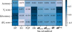
(a)

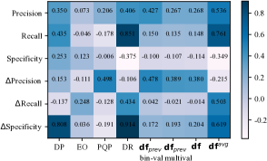
(b)

Figure 1: Correlation heatmap between normal evaluation metric and fairness, for one single sensitive attribute. The used notations refer to those in Table III.

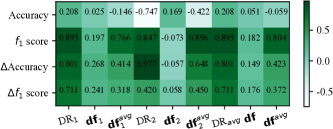
(a)

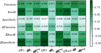
(b)

Figure 2: Correlation heatmap between normal evaluation metric and fairness measure, for all sensitive attributes within the dataset. The notations used here refer to those in Table III.

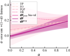
(a)

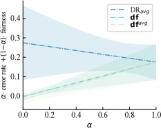
(b)

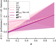
(c)

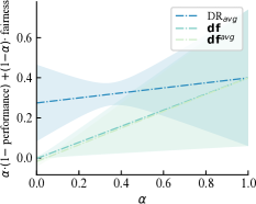
(d)

Figure 3: Plots of best test-set fairness-performance trade-offs per fairness metric [39] (the smaller the better). (a) Plot of fairness-accuracy trade-off for one single sensitive attribute; (b) Plot of fairness-accuracy trade-off for all sensitive attributes; (c–d) Plots of fairness-$\mathrm{f}_{1}$ score trade-off for one sensitive attribute and for all sensitive attributes, respectively. Note that the notations in (a) and (c) refer to those in Table III, and that in (b) and (d) refer to those in Table III.

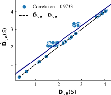
(a)

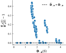
(b)

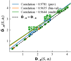
(c)

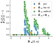
(d)

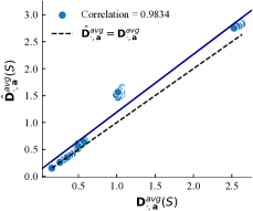
(e)

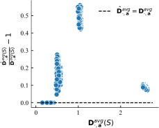
(f)

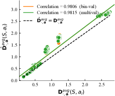
(g)

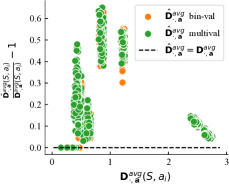
(h)

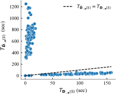
(i)

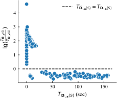
(j)

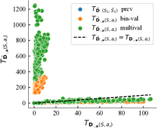
(k)

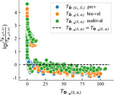
(l)

Figure 4: Comparison of approximation distances between sets with precise distances that are calculated directly by definition, evaluated on test data; Note that ‘prev’ denotes the approximation results obtained by our previous work [34]. (a–b), (c–d), (e–f), and (g–h) Scatter plots for comparison between approximated and precise values of $\mathbf{D}_{\cdot,\bm{a}}^{\text{}}(S)$, $\mathbf{D}_{\cdot,\bm{a}}^{\text{}}(S,a_{i})$, $\mathbf{D}_{\cdot,\bm{a}}^{\text{avg}}(S)$, and $\mathbf{D}_{\cdot,\bm{a}}^{\text{avg}}(S,a_{i})$, respectively; (i–j) Time cost comparison between ExtendDist and direct computation via Eq. (6) and (7); (k–l) Time cost comparison between ApproxDist and direct computation via Eq. (4) and (5).

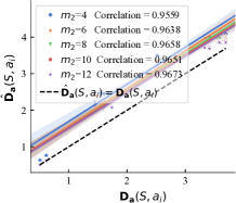
(a)

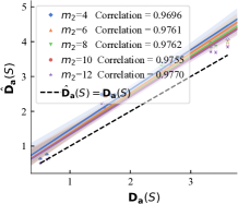
(b)

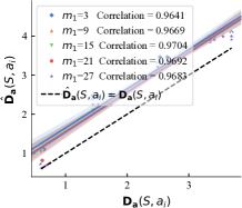
(c)

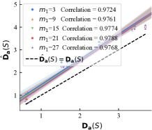
(d)

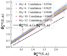
(e)

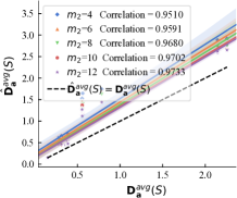
(f)

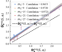
(g)

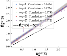
(h)

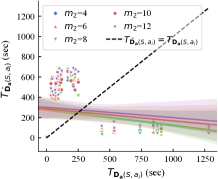
(i)

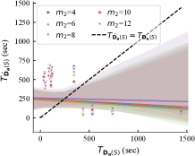
(j)

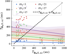
(k)

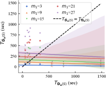
(l)

Figure 5: Effect of hyper-parameters $m_{1}$ and $m_{2}$ in ApproxDist and ExtendDist. (a–b) The effect of $m_{2}$ on the maximal distance value; (c–d) The effect of $m_{1}$ on the maximal distance values. (e–f) The effect of $m_{2}$ on the average distance value; (g–h) The effect of $m_{1}$ on the average distance value. (i–j) The effect of $m_{2}$ on the time cost; (k–l) The effect of $m_{1}$ on the time cost, where $m_{2}$ is set to $\lceil 2\lg(n)\rceil$ in terms of $n$—the size of the corresponding dataset.

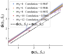
(a)

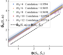
(b)

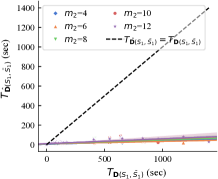
(c)

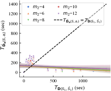
(d)

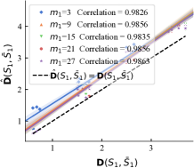
(e)

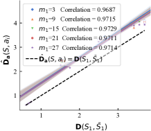
(f)

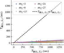
(g)

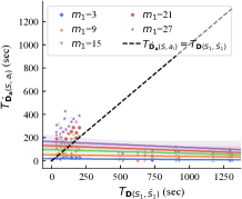
(h)

Figure 6: Effect of hyper-parameters $m_{1}$ and $m_{2}$ in our previous work [34] and ApproxDist here, where only binary values are considered for sensitive attributes. (a–b) The effect of $m_{2}$ on the (maximal) distance value; (c–d) The effect of $m_{2}$ on the time cost. (e–f) The effect of $m_{1}$ on the (maximal) distance value; (g–h) The effect of $m_{1}$ on the time cost, where $m_{2}$ is fixed to $\lceil 2\lg(n)\rceil$ in terms of $n$—the size of the corresponding dataset.

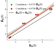
(a)

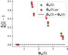
(b)

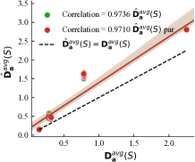
(c)

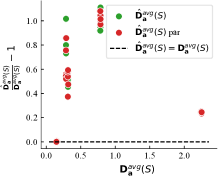
(d)

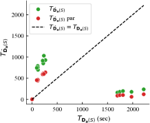
(e)

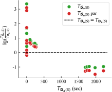
(f)

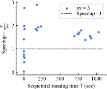
(g)

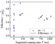
(h)

Figure 7: Comparison of approximation distances between sets with or without integrating parallel computing, where ‘par’ represents results integrating parallel computing and three cores ($m=3$) are used in practice. (a–b) Scatter plots for comparison between approximated values and precise values of $\mathbf{D}_{\mathop{\bm{a}}}(S)$; (c–d) Scatter plots for comparison between approximated values and precise values of $\mathbf{D}_{\mathop{\bm{a}}}^{\text{avg}}(S)$; (e–f) Scatter plots for time cost comparison between obtaining approximation values and obtaining precise values of $\mathbf{D}_{\mathop{\bm{a}}}(S)$ and $\mathbf{D}_{\mathop{\bm{a}}}^{\text{avg}}(S)$; (g–h) Speedup and efficiency for comparison between with and without integrating parallel computing. Note that integrating parallel computing does accelerate the execution of ExtendDist much without sacrificing approximation performance.

Implementation details

We mainly use bagging, AdaBoost, LightGBM [40], FairGBM [39], and AdaFair [41] as learning algorithms, where FairGBM and AdaFair are two fairness-aware ensemble-based methods. Plus, certain kinds of classifiers are used in Section 4.2—including decision trees (DT), naive Bayesian (NB) classifiers, $k$-nearest neighbours (KNN) classifiers, Logistic Regression (LR), support vector machines (SVM), linear SVMs (linSVM), and multilayer perceptrons (MLP)—so that we have a larger learner pools to choose from based on different fairness-relevant rules. Standard 5-fold cross-validation is used in these experiments, in other words, in each iteration, the entire dataset is divided into two parts, with 80% as the training set and 20% as the test set. Also, features of datasets are scaled in preprocessing to lie between 0 and 1. Except for the experiments for RQ3, we set the hyper-parameters $m_{1}=25$ and $m_{2}=\lceil 2\lg(n)\rceil$ in other experiments.

4.2 Comparison between HFM and baseline fairness measures

The aim of this experiment is to evaluate the effectiveness of the proposed HFM compared with baseline fairness measures. As groundtruth discriminative levels of classifiers remain unknown and it is hard to directly compare different methods from that perspective, we compare the correlation (referring to the Pearson correlation coefficient) between the performance difference and different fairness measures. The empirical results are reported in Figures 1–2 and Tables III–III.

For one single sensitive attribute, we can see from Figure 1 that $\mathbf{df}^{\text{avg}}$ is highly correlated with recall/sensitivity and $\mathrm{f}_{1}$ score. Besides, even $\mathbf{df}^{\text{avg}}$ only describes the extra bias, its correlation with $\Delta($performance$)$ is still close to that of DR (and sometimes DP), which means HFM can capture the bias within classifiers indeed and that HFM captures it more finely than our previous work [34]. Moreover, $\mathbf{df}^{\text{avg}}$ shows higher correlation with $\Delta($performance$)$ than $\mathbf{df}$ in most cases, which means $\mathbf{df}^{\text{avg}}$ may capture the extra bias level of classifiers better than $\mathbf{df}$ in practice.

As for multiple sensitive attributes, we can see from Figure 2 that $\mathbf{df}^{\text{avg}}$ is highly correlated with recall/sensitivity and $\mathrm{f}_{1}$ score and that $\mathbf{df}^{\text{avg}}$ shows higher correlation with $\Delta($performance$)$ than $\mathbf{df}$ in most cases, which is similar to our observation in Figure 1. Note that the original DR [32] is only for one single sensitive attributes with binary or multiple values, and for comparison with HFM, we calculate $\text{DR}_{\text{avg}}=\frac{1}{n_{a}}\sum_{i=1}^{n_{a}}\text{DR}_{i}$ here, analogously to $\mathbf{df}^{\text{avg}}$. Besides, we observe that the correlation between $\mathbf{df}^{\text{avg}}$ and $\Delta\text{Accuracy}$ (resp. $\Delta\mathrm{f}_{1}$ score, $\Delta\text{Specificity}$) achieves half of that of DR, and $\mathbf{df}^{\text{avg}}$ even outperforms DR concerning $\Delta\text{Recall}$. Given that HFM only captures the extra bias introduced by classifiers, we believe at least $\mathbf{df}^{\text{avg}}$ could capture quite a part of bias within.

Furthermore, we report plots of fairness-performance trade-offs per fairness measure in Fig. 4. We can see that: 1) for one single sensitive attribute, HFM (i.e., $\mathbf{df}$ and $\mathbf{df}^{\text{avg}}$) achieves the best result in Fig. 4LABEL:sub@subfig:tradeoff,a and 4LABEL:sub@subfig:tradeoff,c; and 2) for all sensitive attributes on one dataset, $\mathbf{df}$ and $\mathbf{df}^{\text{avg}}$ perform closely and both outperform $\text{DR}_{\text{avg}}$ in Fig. 4LABEL:sub@subfig:tradeoff,b and 4LABEL:sub@subfig:tradeoff,d. This observation demonstrates the effectiveness of HFM from another perspective, in other words, HFM could work well if fairness-performance trade-offs need to be considered.

4.3 Validity of approximation algorithms for distances between sets in Euclidean spaces

In this subsection, we evaluate the performance of the proposed ApproxDist and ExtendDist compared with the precise distance that is directly calculated by definitions. To verify whether they could achieve the true distance between sets precisely and timely, we employ scatter plots to compare their values and time cost, presented in Fig. 4. Note that $\mathbf{D}_{\mathbf{a}}^{\text{}}(S,a_{i})$ and $\mathbf{D}_{\mathbf{a}}^{\text{avg}}(S,a_{i})$ are computed together in ApproxDist at one time, and so are $\mathbf{D}_{\mathbf{a}}^{\text{}}(S)$ and $\mathbf{D}_{\mathbf{a}}^{\text{avg}}(S,a_{i})$ in ExtendDist. Also notice that the previous ApproxDist [34] is included for comparison to its current version in scenarios of binary values.

4.3.1 Validity of ApproxDist

As we can see from Figures 4LABEL:sub@subfig:approx,3 and 4LABEL:sub@subfig:approx,4, the approximated values of maximal distance $\mathbf{D}_{\mathbf{a}}^{\text{}}(S,a_{i})$ are highly correlated with their corresponding precise values. Besides, their linear fit line and the identity line (that is, $f(x)=x$) are near and almost parallel, which means the approximated values are pretty close to their precise value. Similar observations are concluded for the average distance $\mathbf{D}_{\mathbf{a}}^{\text{avg}}(S,a_{i})$ shown in Figures 4LABEL:sub@subfig:approx,7 and 4LABEL:sub@subfig:approx,8. As for the execution time of approximation and direct computation in Figures 4LABEL:sub@subfig:approx,11 and 4LABEL:sub@subfig:approx,12, ApproxDist may take a bit longer time in scenarios of multi-value cases than that of binary values, while all of them could achieve a shorter time than precise values when the execution of direct computation is costly.

4.3.2 Validity of ExtendDist

As we can see from Figures 4LABEL:sub@subfig:approx,1 and 4LABEL:sub@subfig:approx,2, the approximated values of maximal distance $\mathbf{D}_{\mathbf{a}}^{\text{}}(S)$ are highly correlated with their corresponding precise values. Besides, their linear fit line and the identity line are near and almost parallel, which means the approximated values are pretty close to their precise value. Similar observations are concluded for the average distance $\mathbf{D}_{\mathbf{a}}^{\text{avg}}(S)$ shown in Figures 4LABEL:sub@subfig:approx,5 and 4LABEL:sub@subfig:approx,6. As for the execution time of approximation and direct computation in Figures 4LABEL:sub@subfig:approx,9 and 4LABEL:sub@subfig:approx,10, ExtendDist would obtain a bigger advantage when computing precise values is expensive, while on the opposite, we do not need ExtendDist that much and can directly calculate them instead.

4.4 Effect of hyper-parameters $m_{1}$ and $m_{2}$

In this subsection, we investigate whether different choices of hyper-parameters (that is, $m_{1}$ and $m_{2}$) would affect the performance of ApproxDist and ExtendDist or not. Different $m_{2}$ values are tested when $m_{1}$ is fixed, and vice versa, with empirical results presented in Figures 6 and 6.

4.4.1 Effect on ApproxDist

As we can see from Figures 6LABEL:sub@subfig:pm,ext,9 and 6LABEL:sub@subfig:pm,ext,11, when direct computation of distances (i.e., maximal distance $\mathbf{D}_{\mathbf{a}}^{\text{}}(S,a_{i})$ and average distance $\mathbf{D}_{\mathbf{a}}^{\text{avg}}(S,a_{i})$) is expensive, obtaining their approximated values via ApproxDist distinctly costs less time than that of precise values by Eq. (4) and (5). Increasing $m_{2}$ (or $m_{1}$) in ApproxDist would cost more time, while the effect of increasing $m_{1}$ is more obvious.

As for the approximation performance of $\mathbf{D}_{\mathbf{a}}^{\text{}}(S,a_{i})$ shown in Fig. 6LABEL:sub@subfig:pm,ext,1 and 6LABEL:sub@subfig:pm,ext,3 as well as approximation performance of $\mathbf{D}_{\mathbf{a}}^{\text{avg}}(S,a_{i})$ shown in Fig. 6LABEL:sub@subfig:pm,ext,5 and 6LABEL:sub@subfig:pm,ext,7, all approximated values are highly correlated and close to the precise values of distance no matter how small $m_{2}$ (or $m_{1}$) is, which means the effect of improper choices of hyper-parameters is unapparent; As $m_{2}$ increases, the approximated values would be closer to the precise values of distance, while the effect of changing $m_{1}$ would be less manifest.

4.4.2 Effect on ExtendDist

As we can see from Figures 6LABEL:sub@subfig:pm,ext,10 and 6LABEL:sub@subfig:pm,ext,12, when direct computation of distances (i.e., maximal distance $\mathbf{D}_{\mathbf{a}}^{\text{}}(S)$ and average distance $\mathbf{D}_{\mathbf{a}}^{\text{avg}}(S)$) is expensive, obtaining their approximated values via ExtendDist distinctly costs less time than that of precise values by Eq. (6) and (7). Increasing $m_{2}$ (or $m_{1}$) in ExtendDist would cost more time, while the effect of increasing $m_{1}$ is more obvious.

As for the approximation performance of $\mathbf{D}_{\mathbf{a}}^{\text{}}(S)$ shown in Figures 6LABEL:sub@subfig:pm,ext,2 and 6LABEL:sub@subfig:pm,ext,4 as well as approximation performance of $\mathbf{D}_{\mathbf{a}}^{\text{avg}}(S)$ shown in Figures 6LABEL:sub@subfig:pm,ext,6 and 6LABEL:sub@subfig:pm,ext,8, all approximated values are highly correlated and close to the precise values of distance no matter how small $m_{2}$ (or $m_{1}$) is, which means the effect of improper choices of hyper-parameters is unapparent; As $m_{2}$ increases, the approximated values would be closer to the precise values of distance, while the effect of changing $m_{1}$ would be less manifest.

4.4.3 Comparison of ApproxDist between our previous work [34] and the current version in this paper

Furthermore, we also present the comparison between our previous work [34] and ApproxDist (Algorithm 2) in Fig. 6.

We can see from Figures 6LABEL:sub@subfig:pm,bin,1, 6LABEL:sub@subfig:pm,bin,2, 6LABEL:sub@subfig:pm,bin,5, and 6LABEL:sub@subfig:pm,bin,6 that our previous ApproxDist demonstrates slightly higher correlation to precise values of maximal distance $\mathbf{D}_{\mathbf{a}}^{\text{}}(S,a_{i})$ (aka. $\mathbf{D}(S_{1},\bar{S}_{1})$ in scenarios of binary values) than its current version in this work; Different choices of $m_{2}$ (or $m_{1}$) cause nearly imperceptible effect on their approximation effectiveness. The previous version also shows close and even better performance on compressed time cost than the current ApproxDist here, depicted in Figures 6LABEL:sub@subfig:pm,bin,3, 6LABEL:sub@subfig:pm,bin,4, 6LABEL:sub@subfig:pm,bin,7, and 6LABEL:sub@subfig:pm,bin,8, especially when direct computation is not much expensive. However, when the execution time cost of direct computation is relatively cheap, ExtendDist displays messy and worse execution speed than ApproxDist, shown in Figures 6LABEL:sub@subfig:pm,ext,11 and 6LABEL:sub@subfig:pm,ext,12. We believe there are mainly two reasons for this phenomenon: one is that AcceleDist is repeated twice from line 2 to line 5 in Algorithm 2 while it is executed only once in the previous ApproxDist [34], causing Algorithm 2 a slightly longer execution time than its previous version; the other is that parallel computing is integrated in ExtendDist in practice to further accelerate its execution, detailed more in Section 4.5 and Figure 7.

4.5 Discussion and limitations

Given the wide applications of ML models in the real world nowadays and the complexity of discrimination mitigation in the face of multiple factors interweaving, it matters a lot to bring in such techniques to deal with several sensitive attributes with even multiple values. Therefore, our work provides a fine-grained fairness measure option named HFM that captures the bias level of models more finely, in order to better detect and moderate discrimination within. The proposed HFM are suitable for both binary and multi-class classification, thus enlarging its applicable value. To promptly approximate the value of HFM, we further proposed ApproxDist and ExtendDist to speed up the expensive calculation process, of which the effectiveness and efficiency have been demonstrated in Section 4.3. However, there are also limitations in the proposed approximation algorithms. The major one is that their time cost will significantly increase if the number of optional values within a sensitive attribute is relatively large. For instance, the computation incurring on the PPR/PPVR datasets may take close or sometimes even longer time than that on the Income dataset, even though the latter has way more instances than the former, because there are six sub-groups under the race attribute on PPR/PPVR while the number is only five on Income. Therefore, we integrate parallel computing in practice to further raise the execution speed of ExtendDist. To be specific, we use three cores to run lines 1 to 3 of Algorithm 1 in parallel in our experiments (Fig. 7), while the choice of the number of cores is not a fixed constant. In other words, using two or four cores is also acceptable if the practitioners like. Furthermore, it is easy to tell that there is still room for improvement in the approximation algorithms. For instance, it might achieve a shorter time of computing in ApproxDist if the procedure between line 1 and line 8 in Algorithm 2 could be executed in parallel, although we did not perform that this time. So does that between line 3 and line 11 of Algorithm 3. But we believe it will need a more deliberate design to balance the parallel computing among them in case the cost of generating more threads/processes to achieve it is not worthy as expected compared with its computing results. Therefore, we would rather leave it in future work, instead of cramming too much and confusing our main contributions in this work.

5 Conclusion

In this paper, we investigate how to evaluate the discrimination level of classifiers in the face of multi-attribute protection scenarios and present a novel harmonic fairness measure with two optional versions (that is, maximum HFM and average HFM), of which both are based on distances between sets from a manifold perspective. To accelerate the computation of distances between sets and reduce its time cost from $\mathcal{O}(n^{2})$ to $\mathcal{O}(n\log n)$, we further propose two approximation algorithms (that is, ApproxDist and ExtendDist) to resolve bias evaluation in scenarios for single attribute protection and multi-attribute protection, respectively. Furthermore, we provide an algorithmic effectiveness analysis for ApproxDist under certain assumptions to explain how well it could work theoretically. The empirical results have demonstrated that the proposed fairness measure (including maximum HFM and average HFM) and approximation algorithms (i.e., ApproxDist and ExtendDist) are valid and effective.

References

- [1] D. Pessach and E. Shmueli, “A review on fairness in machine learning,” ACM Comput Surv, vol. 55, no. 3, pp. 1–44, 2022.
- [2] S. Verma and J. Rubin, “Fairness definitions explained,” in FairWare, 2018, pp. 1–7.
- [3] H. Tian, B. Liu, T. Zhu, W. Zhou, and S. Y. Philip, “Multifair: Model fairness with multiple sensitive attributes,” IEEE Trans Neural Netw Learn Syst, 2024.
- [4] R. Zemel, Y. Wu, K. Swersky, T. Pitassi, and C. Dwork, “Learning fair representations,” in ICML. PMLR, 2013, pp. 325–333.
- [5] H. Xu, X. Liu, Y. Li, A. Jain, and J. Tang, “To be robust or to be fair: Towards fairness in adversarial training,” in ICML, vol. 139. PMLR, 2021, pp. 11 492–11 501.
- [6] M. Padala and S. Gujar, “Fnnc: achieving fairness through neural networks,” in IJCAI, 2021.
- [7] M. Wang and W. Deng, “Mitigating bias in face recognition using skewness-aware reinforcement learning,” in CVPR, 2020, pp. 9322–9331.
- [8] K. Karkkainen and J. Joo, “Fairface: Face attribute dataset for balanced race, gender, and age for bias measurement and mitigation,” in CVPR, 2021, pp. 1548–1558.
- [9] S. Jung, D. Lee, T. Park, and T. Moon, “Fair feature distillation for visual recognition,” in CVPR, 2021, pp. 12 115–12 124.
- [10] F. Locatello, G. Abbati, T. Rainforth, S. Bauer, B. Schölkopf, and O. Bachem, “On the fairness of disentangled representations,” in NeurIPS, vol. 32, 2019.
- [11] M. H. Sarhan, N. Navab, A. Eslami, and S. Albarqouni, “Fairness by learning orthogonal disentangled representations,” in ECCV. Springer, 2020, pp. 746–761.
- [12] D. Guo, C. Wang, B. Wang, and H. Zha, “Learning fair representations via distance correlation minimization,” IEEE Trans Neural Netw Learn Syst, 2022.
- [13] S. Mo, H. Kang, K. Sohn, C.-L. Li, and J. Shin, “Object-aware contrastive learning for debiased scene representation,” in NeurIPS, vol. 34, 2021, pp. 12 251–12 264.
- [14] Y. Roh, K. Lee, S. E. Whang, and C. Suh, “Fairbatch: Batch selection for model fairness,” in ICLR, 2021.
- [15] M. M. Khalili, X. Zhang, and M. Abroshan, “Fair sequential selection using supervised learning models,” in NeurIPS, vol. 34, 2021, pp. 28 144–28 155.
- [16] T. Zhang, T. Zhu, K. Gao, W. Zhou, and S. Y. Philip, “Balancing learning model privacy, fairness, and accuracy with early stopping criteria,” IEEE Trans Neural Netw Learn Syst, vol. 34, no. 9, pp. 5557–5569, 2021.
- [17] S. Hwang and H. Byun, “Unsupervised image-to-image translation via fair representation of gender bias,” in ICASSP. IEEE, 2020, pp. 1953–1957.
- [18] J. Joo and K. Kärkkäinen, “Gender slopes: Counterfactual fairness for computer vision models by attribute manipulation,” in FATE/MM, 2020, pp. 1–5.
- [19] V. V. Ramaswamy, S. S. Kim, and O. Russakovsky, “Fair attribute classification through latent space de-biasing,” in CVPR, 2021, pp. 9301–9310.
- [20] B. Zhao, X. Xiao, G. Gan, B. Zhang, and S.-T. Xia, “Maintaining discrimination and fairness in class incremental learning,” in CVPR, 2020, pp. 13 208–13 217.
- [21] S. Gong, X. Liu, and A. K. Jain, “Mitigating face recognition bias via group adaptive classifier,” in CVPR, 2021, pp. 3414–3424.
- [22] V. Verma, A. Lamb, C. Beckham, A. Najafi, I. Mitliagkas, D. Lopez-Paz, and Y. Bengio, “Manifold mixup: Better representations by interpolating hidden states,” in ICML. PMLR, 2019, pp. 6438–6447.
- [23] H. Zhang, M. Cisse, Y. N. Dauphin, and D. Lopez-Paz, “mixup: Beyond empirical risk minimization,” in ICLR, 2018.
- [24] C.-Y. Chuang and Y. Mroueh, “Fair mixup: Fairness via interpolation,” in ICLR, 2021.
- [25] M. Du, S. Mukherjee, G. Wang, R. Tang, A. Awadallah, and X. Hu, “Fairness via representation neutralization,” in NeurIPS, vol. 34, 2021, pp. 12 091–12 103.
- [26] C. Dwork, M. Hardt, T. Pitassi, O. Reingold, and R. Zemel, “Fairness through awareness,” in ITCS. ACM, 2012, pp. 214–226.
- [27] R. Berk, H. Heidari, S. Jabbari, M. Kearns, and A. Roth, “Fairness in criminal justice risk assessments: The state of the art,” Sociol Methods Res, vol. 50, no. 1, pp. 3–44, 2021.
- [28] I. Žliobaitė, “Measuring discrimination in algorithmic decision making,” Data Min Knowl Discov, vol. 31, no. 4, pp. 1060–1089, 2017.
- [29] M. Joseph, M. Kearns, J. H. Morgenstern, and A. Roth, “Fairness in learning: Classic and contextual bandits,” in NIPS, vol. 29. Curran Associates, Inc., 2016.
- [30] G. Pleiss, M. Raghavan, F. Wu, J. Kleinberg, and K. Q. Weinberger, “On fairness and calibration,” in NIPS, vol. 30, 2017.
- [31] S. Barocas, M. Hardt, and A. Narayanan, Fairness and machine learning: Limitations and opportunities. MIT Press, 2023.
- [32] Y. Bian, K. Zhang, A. Qiu, and N. Chen, “Increasing fairness via combination with learning guarantees,” arXiv preprint arXiv:2301.10813, 2023.
- [33] J. Kang, T. Xie, X. Wu, R. Maciejewski, and H. Tong, “Infofair: Information-theoretic intersectional fairness,” in Big Data. IEEE, 2022, pp. 1455–1464.
- [34] Y. Bian and Y. Luo, “Does machine bring in extra bias in learning? approximating fairness in models promptly,” arXiv preprint arXiv:2405.09251, 2024.
- [35] M. Feldman, S. A. Friedler, J. Moeller, C. Scheidegger, and S. Venkatasubramanian, “Certifying and removing disparate impact,” in SIGKDD, 2015, pp. 259–268.
- [36] P. Gajane and M. Pechenizkiy, “On formalizing fairness in prediction with machine learning,” in FAT/ML, 2018.
- [37] M. Hardt, E. Price, and N. Srebro, “Equality of opportunity in supervised learning,” in NIPS, vol. 29. Curran Associates Inc., 2016, pp. 3323–3331.
- [38] A. Chouldechova, “Fair prediction with disparate impact: A study of bias in recidivism prediction instruments,” Big Data, vol. 5, no. 2, pp. 153–163, 2017.
- [39] A. F. Cruz, C. Belém, J. Bravo, P. Saleiro, and P. Bizarro, “Fairgbm: Gradient boosting with fairness constraints,” in ICLR, 2023.
- [40] G. Ke, Q. Meng, T. Finley, T. Wang, W. Chen, W. Ma, Q. Ye, and T.-Y. Liu, “Lightgbm: A highly efficient gradient boosting decision tree,” in NIPS, vol. 30, 2017, pp. 3146–3154.
- [41] V. Iosifidis and E. Ntoutsi, “Adafair: Cumulative fairness adaptive boosting,” in CIKM. New York, NY, USA: ACM, 2019, pp. 781–790.