Optical RISs Improve the Secret Key Rate of Free-Space QKD in HAP-to-UAV Scenarios

Abstract

Large optical reconfigurable intelligent surfaces (ORISs) are proposed for employment on building rooftops to facilitate free-space quantum key distribution (QKD) between high-altitude platforms (HAPs) and low-altitude platforms (LAPs). Due to practical constraints, the communication terminals can only be positioned beneath the LAPs, preventing direct upward links to HAPs. By deploying ORISs on rooftops to reflect the beam arriving from HAPs towards LAPs from below, reliable HAP-to-LAP links can be established. To accurately characterize the optical beam propagation, we develop an analytical channel model based on extended Huygens-Fresnel principles for representing both the atmospheric turbulence effects and the hovering fluctuations of LAPs. This model facilitates adaptive ORIS beam-width control through linear, quadratic, and focusing phase shifts, which are capable of effectively mitigating the detrimental effects of beam broadening and pointing errors (PE). Furthermore, we derive a closed-form expression for the information-theoretic bound of the QKD secret key rate (SKR) of the HAP-to-LAP links. Our findings demonstrate that quadratic phase shifts enhance the SKR at high HAP-ORIS zenith angles or mild PE conditions by narrowing the beam to optimal sizes. By contrast, linear phase shifts are advantageous at low HAP-ORIS zenith angles under moderate-to-high PE by diverging the beam to mitigate LAP fluctuations.

I Introduction

In parallel to the evolution of cellular systems from the fifth generation (5G) towards the sixth generation (6G), quantum information technology has also experienced rapid growth, particularly in quantum communications. The unconditional security offered by quantum key distribution (QKD) protocols is expected to substantially enhance the communication infrastructure of 6G networks [1]. QKD utilizes quantum states to distribute cryptographic keys between legitimate parties, ensuring that any eavesdropping attempt perturbs the quantum states according to the physical laws of quantum mechanics, thereby revealing the eavesdropper’s presence. QKD protocols are typically categorized as of discrete-variable (DV) and continuous-variable (CV) nature. More specifically, DV-QKD utilizes individual photons for encoding key information, relying on properties like polarizations and requiring single-photon sources as well as detectors [1]. By contrast, CV-QKD maps the key to the quadrature components of Gaussian quantum states, necessitating coherent sources and homodyne/heterodyne detectors [2, 3].

QKD systems have the capability of operating over both optical fiber and free-space optical (FSO) links, but FSO is capable of over-bridging thousands of kilometers from space to ground, eliminating the need for cable installations and relaying [4]. Briefly, fiber-based QKD faces more substantial pathloss in optical fibers than its FSO-based counterpart communicating over atmospheric channels [5]. Recent developments mark a significant shift in quantum network architecture, moving from terrestrial infrastructures to seamless integration with non-terrestrial platforms like unmanned aerial vehicles (UAVs) and satellites, forming essential parts of the Quantum Internet in the Sky [6]. This paradigm shift aligns synergistically with the consideration of non-terrestrial networks (NTNs) in 6G, encompassing low-altitude platforms (LAPs), high-altitude platforms (HAPs), and low-Earth orbit (LEO) satellites [7]. While significant milestones have been reached in establishing quantum links from LEO satellites to the ground [8], research into establishing similar quantum links on other platforms, such as HAPs and LAPs, is in its infancy.

HAPs, relying either on fixed-wing or balloon-based aerial platforms operating at altitudes ranging from 19 km to 22 km in the stratosphere, have been designed for extended quasi-stationary flight powered by solar energy. HAPs can significantly expand the coverage of quantum networks, especially in challenging terrains. On the other hand, LAPs rely on UAVs, such as rotary-wing drones, which operate at altitudes ranging from tens of meters to a few hundred meters, depending on national flight regulations. These platforms offer a flexible and agile infrastructure for quantum communications, making them ideal for rapid deployment in disaster zones and complex urban propagation environments. Recent progress has seen the theoretical exploration of HAPs-to-ground QKD links [9], and the experimental success of both drone-to-ground as well as of drone-to-drone QKD systems [10, 11]. However, the theoretical and experimental performance of HAPs-to-drone QKD links is unknown at the time of writing, leaving a connection gap in the global quantum NTNs.

While it would be desirable to install a communication terminal on top of a drone to establish a direct line-of-sight (LoS) link with HAPs, this is impractical. Explicitly, industrial drones are engineered to carry their payloads underneath using gimbals, which is convenient for optimizing communications with other terminals at similar altitudes or on the ground [10, 11]. The upper part of a drone houses critical components such as batteries, global positioning system (GPS) antennas, and the mechanical frame supporting the drone arms. Mounting equipment on top can interfere with the GPS signal and it is subject to significant vibrations and turbulence from the propellers. Additionally, placing high weight at the top may increase the risk of tipping over, especially in strong winds. By contrast, mounting equipment underneath the drone has the advantage of mitigating vibrations and allows LoS communications with the terminal on the ground. To create reliable QKD links with HAPs, innovative communication methods must be developed that allow the QKD terminal to be installed underneath the drone.

I-A Related Studies

When the direct LoS links between a pair of optical transceivers are blocked or there are hardware alignment difficulties, optical reconfigurable intelligent surfaces (ORISs) [12, 13] have been proposed for both classical [14, 15, 16, 17, 18, 19, 20, 21, 22, 23, 24, 25, 26, 27, 28, 29] and quantum [30, 31] FSO scenarios. Compared to dedicated optical relay nodes, an ORIS offers a cost-effective alternative by using passive elements for controlling the phase of incident beams, hence enabling adaptive beam control and anomalous reflection in specific desired directions at low power consumption [32]. Thanks to its flat surface and compact electronics, an ORIS can be conveniently mounted on building walls or rooftops, typically relying on mirror-array and metasurface types [12, 13]. Briefly, a mirror-array-based ORIS uses small mirrors on micro-electro-mechanical systems (MEMS) to control orientation, while a metasurface-based ORIS utilizes materials having optically modulated properties, like liquid crystals (LC), to produce phase shifts by modulating the molecular alignments.

To elaborate, previous studies typically design ORIS phase-shift profiles and model the optical beam propagation using geometric optics relying on far-field approximations [14, 15, 16, 17, 18, 19, 20, 21, 22, 23, 24, 25, 26]. However, far-field approximations are only valid over distances of dozens of kilometers, which may not be suitable for practical ranges of intermediate-field FSO links. Fortunately, the Huygens-Fresnel (HF) principles have been exploited before for modeling ORIS-assisted FSO channels, which are valid for both intermediate and far fields, spanning distances from dozens of meters to dozens of kilometers [27]. Based on the classic HF principles, both linear phase shift (LPS) and quadratic phase shift (QPS) profiles across the ORIS were considered, where the LPS profile enables anomalous reflection of the beam according to the generalized Snell’s law of reflection, while the QPS profile reduces beam divergence along the propagation path [27]. In designing the QPS profile, specific attention was dedicated both to pointing errors (PEs) arising from random misalignments at the transceivers and ORIS, as well as to beam non-orthogonality [28]. Most recently, a tractable power scaling law based on HF principles has been developed for LPS, QPS, and focusing phase shift (FPS) profiles, offering practical insights into the dependence of received power on the ORIS, on the receiving lens, and on beam widths [29].

The concept of employing ORISs for enhancing non-LoS (NLoS) free-space terrestrial QKD systems was initially introduced in [30]. However, this proposal did not account either for the Gaussian power distribution of the optical beam or for the HF principles. In a recent development, the QPS profile, explicitly considering both the HF principles and the Gaussian power distribution of the optical beam, was investigated in free-space QKD NLoS terrestrial links [31]. Nevertheless, previous seminal studies have overlooked that both the geometric optics and the HF principles only characterize optical beam propagation in free space, i.e., in vacuum [27, 28, 29, 31], but ignore the effects of atmospheric turbulence-induced beam broadening. Furthermore, while random misalignment-induced PEs were explored in [28] based on the HF principles for classical ORIS-aided FSO systems, the corresponding analysis of its QKD counterpart is unavailable in the literature.

I-B Key Contributions

TABLE I: Comparison between this work and the state-of-the-art ORIS-aided classical FSO systems.

Ref.	ORIS Design Principles			Beam Power Distribution		Pointing Errors in 2 Orthogonal Axes			Non- Terrestrial Platforms
	Geometric optics (Far-field distances, vacuum channels)	HF principles (Intermediate & far-field distances, vacuum channels)	Extended HF (EHF) principles (Intermediate & far-field distances, atmospheric channels)	Uniform	Gaussian	Uniform	i.i.d. Gaussian	i.n.i.d. Gaussian
[14, 15]	$\surd$				$\surd$		$\surd$
[16]	$\surd$				$\surd$
[17, 18, 19, 20, 21, 22]	$\surd$				$\surd$		$\surd$
[23, 24, 25]	$\surd$				$\surd$		$\surd$		$\surd$
[26]	$\surd$			$\surd$			$\surd$
[27]		$\surd$			$\surd$
[28]		$\surd$			$\surd$	$\surd$
[29]		$\surd$			$\surd$
This work			$\surd$		$\surd$		$\surd$	$\surd$	$\surd$

TABLE II: Comparison between this work and the state-of-the-art ORIS-aided quantum FSO systems.

Ref.	ORIS Design Principles						Beam Power Distribution		Pointing Errors	Non- Terrestrial Platforms
	HF Principles			EHF Principles			Uniform	Gaussian
	LPS	QPS	FPS	LPS	QPS	FPS
[30]							$\surd$
[31]		$\surd$						$\surd$
This work				$\surd$	$\surd$	$\surd$		$\surd$	$\surd$	$\surd$

In this paper, we propose, for the first time, the utilization of an ORIS for supporting QKD links between HAPs and LAPs. Specifically, an ORIS is strategically positioned on a building rooftop to reflect the signal impinging from HAPs towards LAPs from below. This configuration allows the communication terminal to be installed underneath the LAP. The rooftop positioning is more practical than wall mounting, as it provides unobstructed views and ample space. The LAP is typically an industrial rotary-wing drone capable of carrying substantial payloads [10, 11]. Additionally, ORIS enables adaptive beam-width control through adaptive phase-shift profiles, including LPS, QPS, and FPS. Tables I and II boldly contrast our work against the current state-of-the-art ORIS-aided FSO systems in classical and quantum communication scenarios, respectively. Our contributions in this paper can be summarized in more depth as follows.

• To accurately characterize optical beam propagation over atmospheric channels, we employ the extended HF (EHF) principles [33, 34, 35] to model the effects of atmospheric turbulence-induced beam broadening and various phase-shift profiles on the received beam-width at the LAP. As an extension of the classic HF principles, the EHF principles are applicable to both intermediate-field and far-field distances, covering all practical FSO link ranges. Furthermore, the proposed EHF model accurately characterizes the Gaussian power intensity profile of the FSO beam incident upon the ORIS, which is fundamentally different from the uniform profile of radio-frequency RIS systems. This distinction is crucial for ORIS designs since both classical and quantum FSO systems use a coherent laser source having a Gaussian profile [27, 31].

• The hovering fluctuations of LAPS, caused by GPS inaccuracies or strong winds, lead to significant PEs in the ORIS-to-LAP link. Our analytical framework incorporates these fluctuations in two orthogonal axes by modeling them as two independent but not identically distributed (i.n.i.d.) Gaussian random variables (RVs). We derive a closed-form expression for the statistical geometric and misalignment loss (GML), which is corroborated by Monte-Carlo (MC) simulations. Remarkably, previous studies typically assume simplified PE scenarios associated with independent and identically distributed (i.i.d.) Gaussian RVs in two orthogonal axes [14, 15, 17, 18, 19, 20, 21, 22, 23, 24, 25, 26], or tractable uniformly distributed fluctuations [28]. Our model, therefore, provides a more generalized approach for analyzing the PE of ORIS-aided FSO systems.

• Leveraging the newly developed framework based on EHF principles and generalized PEs, we formulate the ultimate information-theoretic bound of the secret key rate (SKR) in an HAP-ORIS-LAP QKD system. We examine the average Pirandola-Laurenza-Ottaviani-Banchi (PLOB) bound, representing the theoretical upper limit for the SKR of any QKD protocols, including both DV and CV systems. In contrast to previous studies that use a single atmospheric model for all transmission paths [27, 29, 31], we consider independent atmospheric turbulence statistics for the HAP-ORIS and ORIS-LAP paths, giving cognizance to their distinct distances and atmospheric profiles. We extensively investigate all phase-shift profiles, including the LPS, QPS, and FPS, to optimize the received beam-width for mitigating the GML at the LAP, leading to improved SKR under various operational conditions. Thus, we provide a valuable framework for the engineering design of HAP-to-LAP QKD links.

The remainder of this paper is organized as follows. Section II introduces the system and channel models of an ORIS-aided HAP-to-LAP QKD link. In Section III, we develop the analytical framework for modeling the end-to-end GML based on the EHF principles, considering practical ORIS phase-shift profiles and generalized PEs at the LAP. In Section IV, a novel closed-form expression of the PLOB bound is derived for the SKR metric. Detailed numerical results and discussions are provided in Section V. Finally, Section VI concludes the paper.

Notations: Vectors and matrices are represented by boldface lowercase and uppercase letters, respectively; $\left|\cdot\right|$ denotes the absolute value, and $\left\|\mathbf{x}\right\|\!\!\!=\!\!\!\sqrt{x_{1}^{2}\!+\!x_{2}^{2}\!+\!\cdots\!+\!x_{n}^{2}}$ is the norm of a vector $\mathbf{x}\!\!\!=\!\!\!\left(x_{1},x_{2},\!\cdots\!,x_{n}\right)$; $j$ denotes the imaginary unit and $\mathcal{R}\!\left\{\cdot\right\}$ is the real part of a complex number; $\mathbb{E}[\cdot]$ denotes the statistical expectation; $\left\langle\cdot\right\rangle$ represents the ensemble average. $x\!\!\sim\!\!\mathcal{N}(\mu_{x},\sigma_{x}^{2})$ indicates that the RV $x$ follows the Gaussian distribution having statistical mean $\mu_{x}$ and variance $\sigma_{x}^{2}$; $y\!\!\sim\!\!\mathcal{LN}(\mu_{y},\sigma_{y}^{2})$ means that the RV $y$ follows the log-normal distribution with statistical mean $\mu_{y}$ and variance $\sigma_{y}^{2}$. Finally, $\text{erf}\!\left(z\right)\!\!=\!\!\frac{2}{\sqrt{\pi}}\!\int_{0}^{z}\!\exp\!\left(-t^{2}\right)\!\text{d}t$ is the Gaussian error function.

II System and Channel Models

II-A System Model

We investigate a quantum NTN downlink scenario, where a HAP seeks to establish a QKD link with a LAP, specifically with a rotary-wing drone. Due to practical constraints, the QKD terminal is mounted underneath the drone, optimizing communications with other terminals at similar or lower altitudes [10, 11], but impeding signal reception from the HAP. To overcome this limitation, a large ORIS is placed on a building rooftop at a lower altitude than the drone, enabling the reflection of the incoming signal from the HAP towards the drone from below, as depicted in Fig. 1a. The transmitter (Tx) on the HAP is positioned at the origin of the $xyz$-coordinate system at an altitude of $h_{\text{HAP}}$, while the receiver (Rx) on the drone at an altitude of $h_{\text{LAP}}$ is located at the origin of the $x^{\prime}y^{\prime}z^{\prime}$-coordinate system. The center of the ORIS, situated at an altitude of $h_{\text{ORIS}}$, is positioned at the origin of the $x_{\text{r}}y_{\text{r}}z_{\text{r}}$ coordinate system, as illustrated in Fig. 1b, with the horizontal distance from the ORIS center to the projection of LAP on the $x_{\text{r}}y_{\text{r}}$-plane denoted as $d_{\text{LAP}}$. The $x_{\text{r}}y_{\text{r}}$-plane is parallel to the $xz$-plane and the $z_{\text{r}}$-axis is parallel to the $y$-axis. The Tx is equipped with a laser source that emits an optical beam having a Gaussian power density profile. The beam axis transmitted from Tx intersects the $x_{\text{r}}y_{\text{r}}$-plane of the ORIS at a distance $d_{1}$, and it is oriented in the direction $\mathbf{\Psi}_{\text{i}}\!=\!(\theta_{\text{i}},\phi_{\text{i}})$, where $\theta_{\text{i}}$ represents the elevation angle between the $x_{\text{r}}y_{\text{r}}$-plane and the beam axis, while $\phi_{\text{i}}$ denotes the angle between the projection of the beam axis onto the $x_{\text{r}}y_{\text{r}}$-plane and the $x_{\text{r}}$-axis, as depicted in Fig. 1b. In addition, we define $\varphi_{\text{i}}\!=\!90^{\circ}\!-\!\phi_{\text{i}}$ as the zenith angle between the beam axis and the $z_{\text{r}}$-plane. The beam reflected from the ORIS towards the drone at a distance $d_{2}$ is directed towards $\mathbf{\Psi}_{\text{r}}\!=\!(\theta_{\text{r}},\phi_{\text{r}})$, where $\theta_{\text{r}}$ is the angle between the $x_{\text{r}}y_{\text{r}}$-plane and the reflected beam axis. Furthermore, $\phi_{\text{r}}$ denotes the angle between the projection of the reflected beam axis onto the $x_{\text{r}}y_{\text{r}}$-plane and the $x_{\text{r}}$-axis. Similarly, we define $\varphi_{\text{r}}\!=\!90^{\circ}\!-\!\phi_{\text{r}}$ as the zenith angle between the reflected beam axis and the $z_{\text{r}}$-plane.

Similar to [27, 29], without loss of generality, we assume $\phi_{\text{i}}\!\!=\!\!0$ and $\phi_{\text{r}}\!\!=\!\!\pi$ for analytical tractability. Finally, we assume that the Rx communication terminal cannot be mounted on top of the drone due to the space limited by the GPS antennas and owing to the significant vibrations from the propellers (Fig. 1c). Consequently, in practice, it can only be deployed on a 3-axis gimbal attached beneath the drone (Fig. 1d). This practical issue has often been overlooked in the literature. Recent advances in miniaturized optics and engineering have led to the successful development of real-world prototypes for compact communication terminals, which can be installed on various small platforms, such as nanosatellites, HAPs, and drones [37, 38, 39]. This confirms that FSO systems have become a reality for aerial platforms.

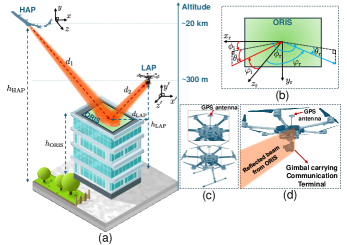
Figure 1: (a) Schematic model of the ORIS-aided HAP-to-LAP QKD link with ORIS deployed on a building rooftop; (b) ORIS coordinates and beam propagation angles; (c) LAP’s top view; (d) LAP’s side view.

We consider an ORIS of size $\sum_{\text{ORIS}}\!\!=\!\!L_{x}\!\!\times\!\!L_{y}$, where $L_{x}$ and $L_{y}$ are the dimensions of the ORIS along the $x_{\text{r}}$- and $y_{\text{r}}$-axes, respectively. This ORIS is of the metasurface type, composed of LC molecules, which act as passive sub-wavelength elements designed to manipulate the properties of the incident beam. Given that typically we have $L_{x},L_{y}\!\gg\!\lambda$, where $\lambda$ is the optical wavelength, a metasurface-based ORIS can be modeled as a continuous surface with continuous phase-shift profiles [29, 31]. For the ORIS designs, we consider the following phase-shift profiles.

• LPS profile: This profile facilitates the generalized Snell’s law of reflection and redirection of the beam from the Tx to the Rx by utilizing an ORIS phase-shift profile that varies linearly along the $x_{\text{r}}$- and $y_{\text{r}}$-axes as follows [27, 29].

  $$\Phi_{\text{ORIS}}^{\text{LP}}\!\left(\mathbf{r}_{\text{r}}\right)=k\left(\Phi_{x}x_{\text{r}}+\Phi_{y}y_{\text{r}}+\Phi_{0}\right),$$ (1)

  where $k=2\pi/\lambda$ denotes the wave number and $\mathbf{r}_{\text{r}}=\left(x_{\text{r}},y_{\text{r}},0\right)$ represents a point in the $x_{\text{r}}y_{\text{r}}$-plane, and $\Phi_{0}$ is constant. The optical beam emerging from Tx in the direction $\mathbf{\Psi}_{\text{i}}$ is redirected to the Rx direction $\mathbf{\Psi}_{\text{r}}$ by applying the phase shift gradients as

  $$\Phi_{x} =\cos\left(\theta_{\text{i}}\right)\cos\left(\phi_{\text{i}}\right)+\cos\left(\theta_{\text{r}}\right)\cos\left(\phi_{\text{r}}\right),$$ (2)

  $$\Phi_{y} =\cos\left(\theta_{\text{i}}\right)\sin\left(\phi_{\text{i}}\right)+\cos\left(\theta_{\text{r}}\right)\sin\left(\phi_{\text{r}}\right).$$ (3)

• QPS profile: This profile focuses the optical beam at a distance $f$ from the ORIS in the direction $\mathbf{\Psi}_{\text{r}}$, reducing the beamwidth of the reflected beam by applying a phase-shift profile that changes quadratically along the $x_{\text{r}}$- and $y_{\text{r}}$-axes as follows [27, 29].

  $$\Phi_{\text{ORIS}}^{\text{QP}}\!\left(\mathbf{r}_{\text{r}}\right)\!=\!k\!\left(\Phi_{x^{2}}x_{\text{r}}^{2}\!+\!\Phi_{y^{2}}y_{\text{r}}^{2}\!+\!\Phi_{x}x_{\text{r}}\!+\!\Phi_{y}y_{\text{r}}\!+\!\Phi_{0}\right)\!,$$ (4)

  where the terms $\Phi_{x^{2}}$ and $\Phi_{y^{2}}$ are given by

  $$\Phi_{x^{2}} =-\frac{\sin^{2}\left(\theta_{\text{i}}\right)}{2R\left(d_{1}\right)}-\frac{\sin^{2}\left(\theta_{\text{r}}\right)}{2d_{2}}+\frac{\sin^{2}\left(\theta_{\text{r}}\right)}{4f}$$ (5)

  $$\Phi_{y^{2}} =-\frac{1}{2R\left(d_{1}\right)}-\frac{1}{2d_{2}}+\frac{1}{4f},$$ (6)

  where $R\left(d_{1}\right)$ is the radius of curvature at the distance $d_{1}$ along the HAP-ORIS path. The term $\frac{1}{4f}$ introduces a parabolic phase profile that narrows the beam at a focus distance $f$. Beyond this point, the beam becomes divergent.

• FPS profile: This profile focuses the optical beam at the Rx, functioning like an artificial lens to concentrate the incident beam at a distance of $d_{2}$ by utilizing the phase-shift profile that eliminates the accumulated phase of the incident beam as follows [27, 29].

  $$\Phi_{\text{ORIS}}^{\text{FP}}=-\psi_{\text{in}}-k\left\|\tilde{\mathbf{r}}_{\text{o}}-\mathbf{r}_{\text{r}}\right\|,$$ (7)

  where $\psi_{\text{in}}$ denotes the phase of the incident beam on the ORIS and $\tilde{\mathbf{r}}_{\text{o}}\!=\!\left(\tilde{x}_{\text{o}},\tilde{y}_{\text{o}},\tilde{z}_{\text{o}}\right)\!=\!\left(-d_{2}\cos\left(\theta_{\text{r}}\right),0,d_{2}\sin\left(\theta_{\text{r}}\right)\right)$ is the center of the Rx aperture.

By applying LPS, QPS, and FPS profiles to ORIS, the width of the beam reflected towards the drone can be controlled to adapt to the channel conditions. Specifically, the LPS profile results in a divergent beam that covers the drone movements under severe hovering fluctuations. The QPS profile offers adaptive control of the reflected beam by adjusting the focus distance $f$, achieving the desired beam pattern at the Rx aperture. This helps to find the optimal beam pattern for achieving the lowest GML in the presence of hovering fluctuation-induced PE and other channel impairments. The FPS profile yields a narrow beam at the Rx aperture, ensuring that most of the power reflected by the ORIS is collected in the absence of hovering fluctuation-induced PE.

II-B Channel Model

In linear quantum optics, the losses can be characterized by the input-output relationship of [41]

$$\hat{a}_{\text{out}}=\sqrt{\tau}\hat{a}_{\text{in}}+\sqrt{1-\tau}\hat{c},$$ (8)

where $\hat{a}_{\text{in}}$ and $\hat{a}_{\text{out}}$ are the input and output field annihilation operators, respectively. Furthermore, $\hat{c}$ is the environmental mode operator in the vacuum state, and $\tau$ is the channel transmittance, characterizing the linear losses within the channel. From (8), $\tau$ is confined to the range of $\left[0,1\right]$ for preserving the canonical commutation relations for the quantized optical field operators in the input-output relationship. In free-space QKD systems, quantum signals are transmitted through atmospheric channels. Consequently, $\tau$ characterizes the fluctuating loss, which is treated as a random variable. The input-output relationship in (8) can be transformed into the Schrodinger picture of motion to derive the corresponding density operators [42]. By employing the Glauber-Sudarshan $P$ representation [43, 44], the relationship between the quantum states transmitted and received through atmospheric channels can be described as [42]

$$P_{\text{out}}\left(\alpha\right)=\int f\!\left(\tau\right)\frac{1}{\tau}P_{\text{in}}\left(\frac{\alpha}{\sqrt{\tau}}\right)\text{d}\tau,$$ (9)

where $P_{\text{in}}\left(\alpha\right)$ and $P_{\text{out}}\left(\alpha\right)$ are the input and output $P$ functions, respectively. Furthermore, $f\!\left(\tau\right)$ denotes the probability distribution of transmittance (PDT). It is deduced from (9) that characterizing quantum signals received from atmospheric channels reduces to the accurate modeling of the PDT. In this paper, the quantum atmospheric channel transmittance $\tau$ is assumed to represent four degradation factors, formulated as

$$\tau=\tau_{\text{eff}}\tau_{\text{l}}I_{\text{a}}\tau_{\text{p}},$$ (10)

where $\tau_{\text{eff}}$ is the Rx efficiency, $\tau_{\text{l}}$ is the deterministic loss over the atmosphere, $I_{\text{a}}$ is the random intensity fluctuation due to atmospheric turbulence, and $\tau_{\text{p}}$ is the GML affected by the ORIS phase-shift profiles and drone hovering fluctuation-induced PE.

For elevation angle $\theta_{\text{i}}>20^{\circ}$, let $\tau_{\text{l,1}}$ denote the atmospheric loss in the HAP-ORIS slanted path, which is scaled as [45]

$$\tau_{\text{l,1}}=\tau_{\text{zen}}^{\sec\left(\varphi_{\text{i}}\right)},$$ (11)

where $\tau_{\text{zen}}$ denotes the transmission efficiency at $\varphi_{\text{i}}\!=\!0^{\circ}$, which can be conveniently estimated by the popular MODTRAN code [45], which is a widely used atmospheric transmittance and radiance simulator. For the ORIS-drone path, assuming $d_{2}\ll d_{1}$ and that the entire $d_{2}$ path is subject to similar atmospheric conditions, we can apply the Beer-Lambert law for estimating the atmospheric loss as [40]

$$\tau_{\text{l,2}}=\exp\left(-\beta_{\text{l}}d_{2}\right),$$ (12)

where $\beta_{\text{l}}$ represents the atmospheric extinction coefficient. With the help of (11) and (12), the atmospheric loss over the HAP-ORIS-drone paths can be calculated as $\tau_{\text{l}}=\tau_{\text{l,1}}\tau_{\text{l,2}}$.

In describing $I_{\text{a}}$, we consider independent atmospheric turbulence-induced intensity fluctuations for the HAP-ORIS and ORIS-drone paths, denoted as $I_{\text{a},1}$ and $I_{\text{a},2}$, respectively. As a result, we have $I_{\text{a}}\!\!=\!\!I_{\text{a},1}I_{\text{a},2}$. In the weak turbulence regime, the log-normal PDT is commonly adopted [33], given by

$$f\!\left(I_{\text{a},\iota}\right)\!=\!\frac{1}{I_{\text{a},\iota}\sqrt{2\pi\sigma_{\text{R},\iota}^{2}}}\exp\!\!\left(\!-\frac{\left(\ln\left(I_{\text{a},\iota}\right)+\frac{\sigma_{\text{R},\iota}^{2}}{2}\right)^{2}}{2\sigma_{\text{R},\iota}^{2}}\!\right)\!,~{}\iota\!\in\!\{1,2\},$$ (13)

where $\sigma_{\text{R},\iota}^{2}$ denotes the Rytov variances for the HAP-ORIS (i.e., $\iota\!=\!1$) and ORIS-drone (i.e., $\iota\!=\!2$) paths over the atmosphere, generally expressed as [33]

$$\sigma_{\text{R},\iota}^{2}\!\!=\!2.25k^{7/6}\!\sec^{11/6}\!\left(\varphi_{\zeta}\right)\!\int_{\!h_{\text{ORIS}}}^{h_{\chi}}\!C_{\text{n}}^{2}\!\left(h\right)\!\!\left(h\!-\!h_{\text{ORIS}}\right)^{5/6}\!\text{d}h,$$ (14)

where $\zeta\!\in\!\{\text{i},\text{r}\}$ and $\chi\!\in\!\{\text{HAP},\text{LAP}\}$ correspond to $\iota\!\in\!\{1,2\}$, respectively. Furthermore, $C_{\text{n}}^{2}\!\left(h\right)$ denotes the refractive index structure parameter, which is determined from the Hufnagel-Valley model as [33]

$$C_{\text{n}}^{2}\!\left(h\right)\!= 0.00594\left(\frac{v}{27}\right)^{\!2}\!\left(10^{-5}h\right)^{\!10}\exp\!\left(\!-\frac{h}{1000}\!\right)$$

$$+2.7\!\times\!10^{-16}\exp\!\left(\!-\frac{h}{1500}\!\right)\!+\!A\exp\!\left(\!-\frac{h}{100}\!\right)\!,$$ (15)

where $h$ is the altitude in meters (m) and $A$ is the nominal value of $C_{\text{n}}^{2}\!\left(0\right)$ at the ground in units of $\text{m}^{-2/3}$. Still referring to (II-B), $v$ (m/s) is the root-mean-squared (rms) transverse wind speed at altitudes above 5 km, readily given by [33]

$$v=\left(\frac{1}{15000}\int_{5000}^{20000}\left[V\!\left(h\right)\right]^{2}\text{d}h\right)^{\!1/2},$$ (16)

where $V\!\left(h\right)$ is the altitude-dependent Greenwood wind profile [46], appropriately modified to include $h_{\text{ORIS}}$ as [47]

$$V\!\left(h\right)=v_{\text{g}}+30\exp\!\left[-\left(\frac{h-12448+h_{\text{ORIS}}}{4800}\right)^{2}\right],$$ (17)

where $v_{\text{g}}$ (m/s) denotes the ground wind speed. To quantify the turbulence strength, the scintillation index, defined as the normalized variance of $I_{\text{a}}$, is widely used. For a downlink path spanning from the HAP to ORIS, a general scintillation index, denoted as $\sigma_{I_{\text{a}}}^{2}$ applicable across all turbulence regimes, is given by [33]

$$\sigma_{I_{\text{a}}}^{2}\!=\!\exp\!\!\left[\!\frac{0.49\sigma_{\text{R},1}^{2}}{\left(1\!+\!1.11\sigma_{\text{R},1}^{12/5}\right)^{\!\!7/6}}\!+\!\frac{0.51\sigma_{\text{R},1}^{2}}{\left(1\!+\!0.69\sigma_{\text{R},1}^{12/5}\right)^{\!\!5/6}}\!\right]\!\!-\!\!1.$$ (18)

The scintillation index serves as a figure of merit indicating the strength of turbulence. Specifically, $\sigma_{I_{\text{a}}}^{2}<1$ indicates a weak turbulence regime, while $\sigma_{I_{\text{a}}}^{2}=1$ represents moderate turbulence, and $\sigma_{I_{\text{a}}}^{2}>1$ denotes strong turbulence conditions [48]. The scintillation index is investigated in Fig. 2 for the dominant HAP-ORIS path versus both the distance $d_{1}$ and the zenith angle $\varphi_{\text{i}}$. The HAP-ORIS distance $d_{1}$ varies with the zenith angle $\varphi_{\text{i}}$ and can be calculated as [48]

$$d_{1}= \sqrt{\left(R_{\text{E}}+h_{\text{HAP}}\right)^{2}+\left(R_{\text{E}}+h_{\text{ORIS}}\right)^{2}\!\left(\cos^{2}\!\left(\varphi_{\text{i}}\right)-1\right)}$$

$$-\left(R_{\text{E}}+h_{\text{ORIS}}\right)\!\cos\!\left(\varphi_{\text{i}}\right),$$ (19)

where $R_{\text{E}}$ denotes the Earth’s radius. In particular, we consider daytime conditions along with $A\!=\!3\!\times\!10^{-13}$ in (II-B) [33], thereby ensuring that the scintillation index depicted in Fig. 2 represents the worst-case scenario for a quantum link. It transpires that $\sigma_{I_{\text{a}}}^{2}\!<\!1$ for $\varphi_{\text{i}}\!\leq\!68^{\circ}$, indicating that this range falls within the weak turbulence regime, which is favorable for quantum communications. However, for $\varphi_{\text{i}}\!>\!68^{\circ}$, the HAP-ORIS link enters the moderate-to-strong turbulence regime, significantly deteriorating the quantum signals and posing substantial challenges for link alignments due to the high zenith angles. Consequently, we restrict the QKD operations to the weak turbulence regime, where $\varphi_{\text{i}}\!\leq\!68^{\circ}$ and $d_{1}\!\leq\!53$ km, ensuring the validity of the log-normal PDT, as experimentally verified for quantum signals in [47].

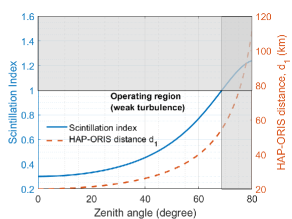
Figure 2: Scintillation index versus HAP-ORIS distance $d_{1}$ and zenith angle $\varphi_{\text{i}}$. $\lambda=810$ nm, $A=3\!\times\!10^{-13}$ $\text{m}^{-2/3}$, $v_{\text{g}}=5$ m/s, $h_{\text{ORIS}}=50$ m, $h_{\text{HAP}}=20$ km, $R_{\text{E}}=6370$ km.

Finally, the GML coefficient $\tau_{\text{p}}$ includes both the deterministic geometrical loss, resulting from the truncation of the receiver aperture capturing only a portion of the optical beam’s power, and the random PE-induced loss caused by drone hovering fluctuations. In ORIS-aided HAP-to-drone QKD links, accurately characterizing the GML is crucial, which is influenced by ORIS phase-shift profiles, atmospheric conditions, and PE due to drone hovering fluctuations. This challenge, unaddressed in the literature, is thoroughly investigated in Section III using the EHF principles, which apply to optical beam propagation over atmospheric channels and practical intermediate-field distances of the ORIS-drone path.

III Statistical GML Based on EHF Principles

III-A Characterization of Optical Beams Using EHF Principles

The impact of ORIS on the incident optical beam can be theoretically modeled using three different frameworks: (i) electromagnetic optics, which relies on vector field descriptions, (ii) wave optics, which uses scalar field descriptions, and (iii) geometric optics. The studies in [27, 29] found that wave optics provides accurate results for practical ORIS-aided FSO systems. Specifically, using scalar fields allows for explicit modeling of arbitrary ORIS phase-shift profiles, ORIS size, and Rx aperture size, which geometric optics fails to achieve. Consequently, the HF principles, based on a scalar-field analysis method, were applied to derive the beam reflected by the ORIS [27, 28, 29]. However, previous studies [27, 28, 29] overlooked that HF principles are only valid for optical beam propagation in a vacuum medium [34]. Particularly, the HF principles state that every point on a wavefront acts as a center of secondary disturbances, producing spherical wavelets, with the wavefront at a later instant becoming the envelope of these wavelets. For a random medium, the EHF principles state that the secondary wavefront is still determined by the envelope of spherical wavelets accruing from the primary wavefront. However, each wavelet is now influenced by the propagation of a spherical wave through the random turbulent medium [34]. Therefore, the key improvement of EHF principles lies in the characterization of turbulence-induced beam broadening and the random component of the complex phase of a spherical wave due to propagation in a turbulent medium [35].

Following [29] and applying the EHF principles [33, 34, 35], the electric field of the Gaussian laser beam incident on the ORIS can be expressed as

$$E_{\text{i}}\!\left(\mathbf{r}_{\text{r}}\right)\!\!=\!\!C_{\text{i}}\!\exp\!\!\left(\!\!-\frac{x_{\text{r}}^{2}}{w_{\text{i},x}^{2}\!\!\left(d_{1}\right)}\!\!-\!\!\frac{y_{\text{r}}^{2}}{w_{\text{i},y}^{2}\!\!\left(d_{1}\right)}\!\!-\!\!j\psi_{\text{i}}\!\left(\mathbf{r}_{\text{r}}\right)\!\!+\!\!\Upsilon\!\left(\mathbf{r}_{\text{r}},d_{1}\right)\!\!\right)\!\!,$$ (20)

with the phase $\psi_{\text{i}}\!\left(\mathbf{r}_{\text{r}}\right)$ given by

$$\psi_{\text{i}}\!\left(\mathbf{r}_{\text{r}}\right)\!=\!k\left(\!\hat{d}_{1}\!+\!\frac{x_{\text{r}}^{2}\sin^{2}\!\left(\theta_{\text{i}}\right)\!+\!y_{\text{r}}^{2}}{2R\!\left(d_{1}\right)}\!\right)\!-\!\tan^{-1}\!\left(\!\frac{d_{1}}{z_{\text{R1}}}\!\right),$$ (21)

where we have $C_{\text{i}}\!=\!\sqrt{\frac{4\eta P_{\text{t}}\left|\sin\left(\theta_{\text{i}}\right)\right|}{\pi w^{2}(d_{1})}}$ and $\eta$ is the channel impedance, $P_{\text{t}}$ is the transmitted power, and $w(d_{1})$ is the beam waist at the distance $d_{1}$. Here, $\hat{d}_{1}\!=\!d_{1}\!-\!x_{\text{r}}\cos\!\left(\theta_{\text{i}}\right)$. $z_{\text{R1}}\!=\!\frac{\pi w_{0}^{2}}{\lambda}$ is the Rayleigh range, which is determined by the beam waist at Tx $w_{0}\!=\!\lambda(\pi\theta_{\text{div}})^{-1}$ along with $\theta_{\text{div}}$ being the Tx half-angle beam divergence. Furthermore, $w_{\text{i},x}\!=\!\frac{w(d_{1})}{\sin\left(\theta_{\text{i}}\right)}$ and $w_{\text{i},x}\!=\!w(d_{1})$ are the indcident beam widths on the ORIS plane in the $x$- and $y$-direction, respectively, while $\Upsilon\!\left(\mathbf{r}_{\text{r}},d_{1}\right)$ denotes the phase pertubation of the field due to random inhomogeneities along the HAP-ORIS path. Subsequently, the electric field of the beam reflected by the ORIS and received at the Rx aperture of the drone can be written as

$$E_{\text{r}}\!\left(\mathbf{r}^{\prime}\right)\!=\!C_{\text{r}}\! \iint_{\left(x_{\text{r}},y_{\text{r}}\in\sum_{\text{ORIS}}\right)}\!E_{\text{i}}\!\left(\mathbf{r}_{\text{r}}\right)\exp\!\left(-jk\left\|\mathbf{r}_{\text{o}}\!-\!\mathbf{r}_{\text{r}}\right\|\right)$$

$$\times\!\exp\!\left[-j\Phi_{\text{ORIS}}\!\left(\mathbf{r}_{\text{r}}\right)\right]\exp\!\left(\Upsilon\!\left(\mathbf{r}^{\prime},d_{2}\right)\right)\!,$$ (22)

where $C_{\text{r}}\!=\!\frac{\sqrt{\sin\left(\theta_{\text{r}}\right)}}{j\lambda d_{2}}$, $\mathbf{r}_{\text{o}}\!=\!\left(\mathbf{r}^{\prime}\!+\!\mathbf{c}\right)\mathbf{R}_{\text{rot}}$ with $\mathbf{r}^{\prime}\!=\!\left(x^{\prime},y^{\prime},z^{\prime}\right)$ being a point in the Rx aperture plane and $\mathbf{c}=\left(0,0,d_{2}\right)$. Furthermore, we have a rotation matrix of

$$\mathbf{R}_{\text{rot}}=\begin{pmatrix}-\sin\!\left(\theta_{\text{r}}\right)&0&-\cos\!\left(\theta_{\text{r}}\right)\\ 0&-1&0\\ -\cos\!\left(\theta_{\text{r}}\right)&0&\sin\!\left(\theta_{\text{r}}\right)\end{pmatrix},$$ (23)

and $E_{\text{i}}\!\left(\mathbf{r}_{\text{r}}\right)$ of (III-A) is given in (20), while $\Upsilon\!\left(\mathbf{r}^{\prime},d_{2}\right)$ denotes the phase perturbation of the field due to random inhomogeneities along the ORIS-drone path.

In characterizing wave propagation through atmospheric turbulence, the statistical long-term-average moments of the optical field are of great interest. Thus, the mean electric field of $E_{\text{r}}\!\left(\mathbf{r}^{\prime}\right)$ can be written with the help of (20) and (III-A) as

$$\left\langle E_{\text{r}}\!\left(\mathbf{r}^{\prime}\right)\right\rangle\!\!=\!\!C_{\text{r}}C_{\text{i}}\! \iint_{\!\left(\!x_{\text{r}},y_{\text{r}}\in\sum_{\text{ORIS}}\!\right)}\!\!\!\exp\!\!\left(\!\!-\frac{x_{\text{r}}^{2}}{w_{\text{i},x}^{2}\!\!\left(\!d_{1}\!\right)}\!-\!\frac{y_{\text{r}}^{2}}{w_{\text{i},y}^{2}\!\!\left(\!d_{1}\!\right)}\!-\!j\psi_{\text{i}}\!\left(\mathbf{r}_{\text{r}}\right)\!\!\right)$$

$$\times\exp\!\left(-jk\left\|\mathbf{r}_{\text{o}}\!-\!\mathbf{r}_{\text{r}}\right\|\right)\exp\!\left(\!-j\Phi_{\text{ORIS}}\!\left(\mathbf{r}_{\text{r}}\right)\!\right)$$

$$\times\left\langle\exp\!\left[\Upsilon\!\left(\mathbf{r}_{\text{r}},d_{1}\right)\right]\right\rangle\left\langle\exp\!\left[\Upsilon\!\left(\mathbf{r}^{\prime},d_{2}\right)\right]\right\rangle.$$ (24)

To calculate the ensemble averages appearing in (III-A), we invoke the relationship [33]

$$\left\langle\exp\!\left(\Upsilon\right)\right\rangle\!=\!\exp\!\!\left[\!\left\langle\Upsilon\right\rangle\!+\!\frac{1}{2}\!\left(\!\left\langle\Upsilon^{2}\right\rangle\!-\!\left\langle\Upsilon\right\rangle^{\!2}\!\right)\!\right]\!\!=\!\exp\!\left[E_{1}\!\!\left(0,0\right)\right],$$ (25)

which leads to the relationship with the second-order statistical moment of the optical field $E_{1}\!\left(0,0\right)$ that is real and independent of the observation point and the matrix elements between the input and output planes [33]. As a result, $\left\langle\exp\!\left[\Upsilon\!\left(\mathbf{r}_{\text{r}},d_{1}\right)\right]\right\rangle$ and $\left\langle\exp\!\left[\Upsilon\!\left(\mathbf{r}^{\prime},d_{2}\right)\right]\right\rangle$ in (III-A) can be respectively formulated as [33]

$$\left\langle\exp\!\left[\Upsilon\!\left(\!\mathbf{r}_{\text{r}},d_{1}\!\right)\right]\right\rangle\!\! =\!\!\exp\!\!\left[\!-2\pi^{2}k^{2}\!\sec\!\left(\!\varphi_{\text{i}}\!\right)\!\!\int_{h_{\text{ORIS}}}^{h_{\text{HAP}}}\!\!\!\int_{0}^{\infty}\!\!\kappa\Phi_{n}\!\!\left(\!\kappa,h\!\right)\!\right]\!\!\text{d}\kappa\text{d}h,$$ (26)

$$\left\langle\exp\!\left[\Upsilon\!\left(\!\mathbf{r}^{\prime},d_{2}\!\right)\right]\right\rangle\!\! =\!\!\exp\!\!\left[\!-2\pi^{2}k^{2}\!\sec\!\left(\!\varphi_{\text{r}}\!\right)\!\!\int_{h_{\text{ORIS}}}^{h_{\text{LAP}}}\!\!\!\int_{0}^{\infty}\!\!\kappa\Phi_{n}\!\!\left(\!\kappa,h\!\right)\!\right]\!\!\text{d}\kappa\text{d}h,$$ (27)

where $\Phi_{n}\!\left(\!\kappa,h\!\right)$ denotes the spectral density of the refractive index fluctuations, with $\kappa$ being the scalar magnitude of the three-dimensional spatial wave number vector $\mathbf{K}$, under the assumption that the random medium is statistically homogeneous and isotropic in each transversal plane [33]. It is observed that the mean fields $\left\langle\exp\!\left[\Upsilon\!\left(\mathbf{r}_{\text{r}},d_{1}\right)\right]\right\rangle$ and $\left\langle\exp\!\left[\Upsilon\!\left(\mathbf{r}^{\prime},d_{2}\right)\right]\right\rangle$ in (26) and (27), respectively, tend to zero for both visible and infrared wavelengths due to the $k^{2}$ term. Hence, the impact of phase perturbation becomes negligible for our QKD links at $\lambda\!=\!810$ nm.

To this end, the effect of atmospheric turbulence reduces to beam broadening in both the HAP-ORIS and ORIS-drone links, which was not considered in previous studies [27, 28, 29]. The beam broadening effect of the HAP-ORIS path can be characterized by $w(d_{1})$, which represents the long-term beam waist at a distance $d_{1}$ after propagating through the atmosphere. Assuming a Tx collimated beam, $w(d_{1})$ is given by [33]

$$w(d_{1})\!=\!w_{0}\sqrt{\left(1\!+\!\Lambda_{0}^{2}\right)\left(1\!+\!T\right)},$$ (28)

where we have $\Lambda_{0}\!=\!\frac{2d_{1}}{kw_{0}^{2}}$, and $T$ characterizes the turbulence-induced beam broadening effect, expressed as [33]

$$T= 4.35\Lambda^{5/6}k^{7/6}\left(h_{\text{HAP}}-h_{\text{ORIS}}\right)^{5/6}\sec^{11/6}\!\left(\varphi_{\text{i}}\right)$$

$$\times\int_{h_{\text{ORIS}}}^{h_{\text{HAP}}}C_{\text{n}}^{2}\!\left(h\right)\!\left(\frac{h-h_{\text{ORIS}}}{h_{\text{HAP}}-h_{\text{ORIS}}}\right)^{\!5/3}\text{d}h,$$ (29)

where $\Lambda=\frac{\Lambda_{0}}{1+\Lambda_{0}^{2}}$. Upon using the parameters provided in the caption of Fig. 2 along with $\theta_{\text{div}}=16.5$ $\mu$rad for a collimated beam [47], and substituting them into (28) and (III-A), we find that the maximum beam widths incident on the ORIS are $w_{\text{i},x}\!=\!36.81$ cm and $w_{\text{i},y}\!=\!34.14$ cm at $\varphi_{\text{i}}\!=\!68^{\circ}$. This results in an elliptical beam with major and minor diameters of 73.62 m and 68.28 m, respectively. Given that the ORIS is fixed on the building rooftop, the Tx is equipped with an accurate pointing system [39], and the ORIS size exceeds the beam footprint, the PE in the HAP-ORIS link thus can be considered negligible. To ensure that the incident beam footprint remains well within the large ORIS, the dimensions of $\sum_{\text{ORIS}}$ in this paper should be $L_{x}\!=\!L_{y}\!=\!1$ m. For the ORIS-drone path, the turbulence-induced beam broadening effect must be considered when calculating the beam widths at the Rx aperture for different ORIS phase-shift profiles. This is discussed in Section III-B.

III-B GML With ORIS Phase-Shift Profiles and Drone Hovering Fluctuations

The GML coefficient $\tau_{\text{p}}$ is defined as [29]

$$\tau_{\text{p}}=\frac{1}{2\eta P_{\text{t}}}\iint_{\mathcal{A}_{\text{Rx}}}\left|\left\langle E_{\text{r}}\!\left(\mathbf{r}^{\prime}\right)\right\rangle\right|^{2}\text{d}\mathcal{A}_{\text{Rx}},$$ (30)

where $\mathcal{A}_{\text{Rx}}$ denotes the area of the Rx aperture and $\left\langle E_{\text{r}}\!\left(\mathbf{r}^{\prime}\right)\right\rangle$ is given in (III-A). Following the approach in [29], we derive closed-form solutions for (30) to estimate $\tau_{\text{p}}$, which depends on different ORIS phase-shift profiles and $\mathcal{A}_{\text{Rx}}$. Assuming that $\sum_{\text{ORIS}}\gg A_{\text{in}}$, where $A_{\text{in}}=\pi w_{\text{i},x}w_{\text{i},y}$ represents the area of the equivalent beam footprint incident on the ORIS, $\tau_{\text{p}}$ follows the saturated power scaling regime [29], where all the power of the incident beam on the ORIS is reflected towards the drone. Thus, $\tau_{\text{p}}$ is independent of $\sum_{\text{ORIS}}$ and characterized by the GML governed by the Rx beam footprint, $\mathcal{A}_{\text{Rx}}$, and the average PE loss imposed by drone hovering fluctuations.

Lemma 1.

Using the LPS profile in (1) and assuming that the hovering fluctuations in positions of the drone in $x^{\prime}$ and $y^{\prime}$ axes, respectively denoted as $\tilde{x}^{\prime}$ and $\tilde{y}^{\prime}$, are i.n.i.d. Gaussian RVs, i.e., $\tilde{x}^{\prime}\!\sim\!\mathcal{N}(\mu_{\tilde{x}^{\prime}},\sigma_{\tilde{x}^{\prime}}^{2})$ and $\tilde{y}^{\prime}\!\sim\!\mathcal{N}(\mu_{\tilde{y}^{\prime}},\sigma_{\tilde{y}^{\prime}}^{2})$, the statistical average GML coefficient $\tau_{\text{p}}$ can be approximated by $\tau_{\text{p}}^{\text{LPS}}$, as given in (31) shown at the bottom of this page. In (31), $a$ denotes the radius of the Rx aperture, while $w_{\text{rx},x^{\prime}}^{\text{LPS}}\!=\!w\!\left(d_{1}\right)\!\frac{\left|\sin\left(\theta_{\text{r}}\right)\right|}{\left|\sin\left(\theta_{\text{i}}\right)\right|}\sqrt{\varepsilon\left(\frac{\sin^{2}\left(\theta_{\text{i}}\right)}{\sin^{2}\left(\theta_{\text{r}}\right)}\Lambda_{1}\right)^{\!2}\!+\!1}$ and $w_{\text{rx},y^{\prime}}^{\text{LPS}}\!=\!w\!\left(d_{1}\right)\!\sqrt{\varepsilon\Lambda_{1}^{2}\!+\!1}$ are the equivalent beam widths given by the LPS profile at the Rx aperture in the $x^{\prime}$ and $y^{\prime}$ axes, respectively. Finally, $\Lambda_{1}\!=\!\frac{2d_{2}}{kw^{2}(d_{1})}$ and $\varepsilon=1\!+\!\frac{2w^{2}(d_{1})}{\rho_{0}^{2}}$, with $\rho_{0}\!=\!\left(1.45k^{2}\!\int_{h_{\text{ORIS}}}^{h_{\text{LAP}}}C_{\text{n}}^{2}\!\left(h\right)\text{d}h\right)^{\!-3/5}\!\cos^{3/5}\!\left(\varphi_{\text{r}}\right)$.

 

$$\tau_{\text{p}}^{\text{LPS}}\!=\!\frac{1}{4}\!\left[\!\text{erf}\!\left(\!\frac{\frac{\mu_{\tilde{x}^{\prime}}}{\sqrt{2}w_{\text{rx},x^{\prime}}^{\text{LPS}}}\!+\!\frac{a\sqrt{\pi}}{2w_{\text{rx},x^{\prime}}^{\text{LPS}}}}{\sqrt{1\!+\!\frac{\sigma_{\tilde{x}^{\prime}}^{2}}{\left(\!w_{\text{rx},x^{\prime}}^{\text{LPS}}\!\right)^{\!2}}}}\!\right)\!\!\!-\!\text{erf}\!\left(\!\frac{\frac{\mu_{\tilde{x}^{\prime}}}{\sqrt{2}w_{\text{rx},x^{\prime}}^{\text{LPS}}}\!-\!\frac{a\sqrt{\pi}}{2w_{\text{rx},x^{\prime}}^{\text{LPS}}}}{\sqrt{1\!+\!\frac{\sigma_{\tilde{x}^{\prime}}^{2}}{\left(\!w_{\text{rx},x^{\prime}}^{\text{LPS}}\!\right)^{\!2}}}}\!\right)\!\right]\!\!\left[\!\text{erf}\!\left(\!\frac{\frac{\mu_{\tilde{y}^{\prime}}}{\sqrt{2}w_{\text{rx},y^{\prime}}^{\text{LPS}}}\!+\!\frac{a\sqrt{\pi}}{2w_{\text{rx},y^{\prime}}^{\text{LPS}}}}{\sqrt{1\!+\!\frac{\sigma_{\tilde{y}^{\prime}}^{2}}{\left(\!w_{\text{rx},y^{\prime}}^{\text{LPS}}\!\right)^{\!2}}}}\!\right)\!\!\!-\!\text{erf}\!\left(\!\frac{\frac{\mu_{\tilde{y}^{\prime}}}{\sqrt{2}w_{\text{rx},y^{\prime}}^{\text{LPS}}}\!-\!\frac{a\sqrt{\pi}}{2w_{\text{rx},y^{\prime}}^{\text{LPS}}}}{\sqrt{1\!+\!\frac{\sigma_{\tilde{y}^{\prime}}^{2}}{\left(\!w_{\text{rx},y^{\prime}}^{\text{LPS}}\!\right)^{\!2}}}}\!\right)\!\right]\!\!.$$ (31)

Proof.

See Appendix A. ∎

Remark 1.

From Lemma 1, we observe that $\Lambda_{1}$ quantifies the increase in beam width along the ORIS-drone path at a distance $d_{2}$ solely caused by diffraction. In addition, $\varepsilon$ characterizes the beam broadening due to atmospheric turbulence after reflection by the ORIS. In the absence of atmospheric turbulence, i.e., in a vacuum, $\rho_{0}\rightarrow\infty$ and $\varepsilon\rightarrow 1$. Hence, under these conditions, the beam broadening is governed purely by free-space diffraction, as described by $\Lambda_{1}$.

Lemma 2.

Using the QPS profile in (4) and assuming that the hovering fluctuations in positions of the drone in $x^{\prime}$ and $y^{\prime}$ axes, respectively denoted as $\tilde{x}^{\prime}$ and $\tilde{y}^{\prime}$, are i.n.i.d. Gaussian RVs, i.e., $\tilde{x}^{\prime}\!\sim\!\mathcal{N}(\mu_{\tilde{x}^{\prime}},\sigma_{\tilde{x}^{\prime}}^{2})$ and $\tilde{y}^{\prime}\!\sim\!\mathcal{N}(\mu_{\tilde{y}^{\prime}},\sigma_{\tilde{y}^{\prime}}^{2})$, the statistical average GML coefficient $\tau_{\text{p}}$ can be approximated by $\tau_{\text{p}}^{\text{QPS}}$, as given in (32) shown at the bottom of this page. In (32), $w_{\text{rx},x^{\prime}}^{\text{QPS}}\!=\!w\!\left(d_{1}\right)\!\frac{\left|\sin\left(\theta_{\text{r}}\right)\right|}{\left|\sin\left(\theta_{\text{i}}\right)\right|}\sqrt{\varepsilon\!\left(\frac{\sin^{2}\left(\theta_{\text{i}}\right)}{\sin^{2}\left(\theta_{\text{r}}\right)}\Lambda_{1}\right)^{\!2}\!+\!\left(\frac{d_{2}}{2f}\right)^{\!2}}$ and $w_{\text{rx},y^{\prime}}^{\text{QPS}}\!=\!w\!\left(d_{1}\right)\!\sqrt{\varepsilon\Lambda_{1}^{2}\!+\!\left(\frac{d_{2}}{2f}\right)^{\!2}}$ are the equivalent beam widths induced by the QPS profile at the Rx aperture in the $x^{\prime}$ and $y^{\prime}$ axes, respectively. Finally, $a$, $\varepsilon$, and $\rho_{0}$ are defined in Lemma 1.

$$\tau_{\text{p}}^{\text{QPS}}\!=\!\frac{1}{4}\!\left[\!\text{erf}\!\left(\!\frac{\frac{\mu_{\tilde{x}^{\prime}}}{\sqrt{2}w_{\text{rx},x^{\prime}}^{\text{QPS}}}\!+\!\frac{a\sqrt{\pi}}{2w_{\text{rx},x^{\prime}}^{\text{QPS}}}}{\sqrt{1\!+\!\frac{\sigma_{\tilde{x}^{\prime}}^{2}}{\left(\!w_{\text{rx},x^{\prime}}^{\text{QPS}}\!\right)^{\!2}}}}\!\right)\!\!\!-\!\text{erf}\!\left(\!\frac{\frac{\mu_{\tilde{x}^{\prime}}}{\sqrt{2}w_{\text{rx},x^{\prime}}^{\text{QPS}}}\!-\!\frac{a\sqrt{\pi}}{2w_{\text{rx},x^{\prime}}^{\text{QPS}}}}{\sqrt{1\!+\!\frac{\sigma_{\tilde{x}^{\prime}}^{2}}{\left(\!w_{\text{rx},x^{\prime}}^{\text{QPS}}\!\right)^{\!2}}}}\!\right)\!\right]\!\!\left[\!\text{erf}\!\left(\!\frac{\frac{\mu_{\tilde{y}^{\prime}}}{\sqrt{2}w_{\text{rx},y^{\prime}}^{\text{QPS}}}\!+\!\frac{a\sqrt{\pi}}{2w_{\text{rx},y^{\prime}}^{\text{QPS}}}}{\sqrt{1\!+\!\frac{\sigma_{\tilde{y}^{\prime}}^{2}}{\left(\!w_{\text{rx},y^{\prime}}^{\text{QPS}}\!\right)^{\!2}}}}\!\right)\!\!\!-\!\text{erf}\!\left(\!\frac{\frac{\mu_{\tilde{y}^{\prime}}}{\sqrt{2}w_{\text{rx},y^{\prime}}^{\text{QPS}}}\!-\!\frac{a\sqrt{\pi}}{2w_{\text{rx},y^{\prime}}^{\text{QPS}}}}{\sqrt{1\!+\!\frac{\sigma_{\tilde{y}^{\prime}}^{2}}{\left(\!w_{\text{rx},y^{\prime}}^{\text{QPS}}\!\right)^{\!2}}}}\!\right)\!\right]\!\!.$$ (32)

Proof.

See Appendix B. ∎

Remark 2.

Lemma 2 reveals that increasing the focus distance $f$ results in a smaller beam footprint at the Rx aperture plane. Consequently, by adaptively adjusting $f$, the beam width at the receiver can be optimized for enhancing the performance under varying PE severities caused by drone hovering fluctuations. In the absence of atmospheric turbulence-induced beam broadening, where $\varepsilon\rightarrow 1$, (32) reduces to [29, (24)]. Additionally, by comparing (32) and (31), we find that setting $f\!=\!d_{2}/2$ causes an ORIS with a QPS profile to behave identically to one with a LPS profile.

Lemma 3.

Using the FPS profile in (7) and assuming that the hovering fluctuations in positions of the drone in $x^{\prime}$ and $y^{\prime}$ axes, respectively denoted as $\tilde{x}^{\prime}$ and $\tilde{y}^{\prime}$, are i.n.i.d. Gaussian RVs, i.e., $\tilde{x}^{\prime}\!\sim\!\mathcal{N}(\mu_{\tilde{x}^{\prime}},\sigma_{\tilde{x}^{\prime}}^{2})$ and $\tilde{y}^{\prime}\!\sim\!\mathcal{N}(\mu_{\tilde{y}^{\prime}},\sigma_{\tilde{y}^{\prime}}^{2})$, the statistical average GML coefficient $\tau_{\text{p}}$ can be approximated by $\tau_{\text{p}}^{\text{FPS}}$, as given in (33) shown at the bottom of the next page. In (33), $w_{\text{rx},x^{\prime}}^{\text{FPS}}\!=\!w\!\left(d_{1}\right)\!\frac{\left|\sin\left(\theta_{\text{i}}\right)\right|}{\left|\sin\left(\theta_{\text{r}}\right)\right|}\sqrt{\varepsilon\Lambda_{1}^{2}}$ and $w_{\text{rx},y^{\prime}}^{\text{FPS}}\!=\!w\!\left(d_{1}\right)\!\sqrt{\varepsilon\Lambda_{1}^{2}}$ are the equivalent beam widths induced by the FPS profile at the Rx aperture in the $x^{\prime}$ and $y^{\prime}$ axes, respectively. Furthermore, $a$, $\varepsilon$, and $\rho_{0}$ are defined in Lemma 1.

 

$$\tau_{\text{p}}^{\text{FPS}}\!=\!\frac{1}{4}\!\left[\!\text{erf}\!\left(\!\frac{\frac{\mu_{\tilde{x}^{\prime}}}{\sqrt{2}w_{\text{rx},x^{\prime}}^{\text{FPS}}}\!+\!\frac{a\sqrt{\pi}}{2w_{\text{rx},x^{\prime}}^{\text{FPS}}}}{\sqrt{1\!+\!\frac{\sigma_{\tilde{x}^{\prime}}^{2}}{\left(\!w_{\text{rx},x^{\prime}}^{\text{FPS}}\!\right)^{\!2}}}}\!\right)\!\!\!-\!\text{erf}\!\left(\!\frac{\frac{\mu_{\tilde{x}^{\prime}}}{\sqrt{2}w_{\text{rx},x^{\prime}}^{\text{FPS}}}\!-\!\frac{a\sqrt{\pi}}{2w_{\text{rx},x^{\prime}}^{\text{FPS}}}}{\sqrt{1\!+\!\frac{\sigma_{\tilde{x}^{\prime}}^{2}}{\left(\!w_{\text{rx},x^{\prime}}^{\text{FPS}}\!\right)^{\!2}}}}\!\right)\!\right]\!\!\left[\!\text{erf}\!\left(\!\frac{\frac{\mu_{\tilde{y}^{\prime}}}{\sqrt{2}w_{\text{rx},y^{\prime}}^{\text{FPS}}}\!+\!\frac{a\sqrt{\pi}}{2w_{\text{rx},y^{\prime}}^{\text{FPS}}}}{\sqrt{1\!+\!\frac{\sigma_{\tilde{y}^{\prime}}^{2}}{\left(\!w_{\text{rx},y^{\prime}}^{\text{FPS}}\!\right)^{\!2}}}}\!\right)\!\!\!-\!\text{erf}\!\left(\!\frac{\frac{\mu_{\tilde{y}^{\prime}}}{\sqrt{2}w_{\text{rx},y^{\prime}}^{\text{FPS}}}\!-\!\frac{a\sqrt{\pi}}{2w_{\text{rx},y^{\prime}}^{\text{FPS}}}}{\sqrt{1\!+\!\frac{\sigma_{\tilde{y}^{\prime}}^{2}}{\left(\!w_{\text{rx},y^{\prime}}^{\text{FPS}}\!\right)^{\!2}}}}\!\right)\!\right]\!\!.$$ (33)

Proof.

See Appendix C. ∎

Remark 3.

Lemma 3 demonstrates that the beam footprint at the receiver is significantly smaller than those described in Lemmas 1 and 2. In the absence of atmospheric turbulence-induced beam broadening, where $\varepsilon\rightarrow 1$, (33) simplifies to [29, (25)] and the beam footprint is on the order of $w_{0}$, which is much smaller than the Rx aperture radius $a$, leading to $\tau_{\text{p}}^{\text{FPS}}\approx 0$ dB. Furthermore, by comparing (33) and (32), we find that setting $f\!=\!\infty$ in (32) makes an ORIS with a QPS profile behave identically to one with a FPS profile.

IV Bounding the SKR of QKD Systems

Optical communications over free-space links inherently experience channel impairments, which can be typically characterized by the transmissivity coefficient $\tau$ defined in (10), quantifying the fraction of input photons that “survive” the channel. For a lossy channel having arbitrary transmissivity $\tau$, the PLOB bound establishes the ultimate information-theoretic upper limit for the SKR of any DV/CV-QKD protocols [31, 48, 51], given by

$$\mathfrak{R}\!\leq\!-\log_{2}\!\left(1-\tau\right)\!=\!-\log_{2}\!\left(1-\tau_{\text{eff}}\tau_{\text{l}}I_{\text{a}}\tau_{\text{p}}\right).$$ (34)

Due to atmospheric turbulence-induced intensity fluctuations in transmissivity $\tau$ caused by $I_{\text{a}}$, the average PLOB bound of the SKR $\mathfrak{R}$ over the HAP-ORIS and ORIS-drone links can be expressed as

$$\mathfrak{R}\!\leq\!\int_{0}^{1/\tau_{\text{eff}}\tau_{\text{l}}\tau_{\text{p}}}\!-\log_{2}\!\left(1\!-\!\tau_{\text{eff}}\tau_{\text{l}}I_{\text{a}}\tau_{\text{p}}\right)\!f\!\left(I_{\text{a},1}\right)\!f\!\left(I_{\text{a},2}\right)\!\text{d}I_{\text{a},1}\text{d}I_{\text{a},2},$$ (35)

where $f\!\left(I_{\text{a},\iota}\right)$ with $\iota\!\in\!\{1,2\}$ is the log-normal PDT defined in (13).

Corollary 1.

A closed-form expression of the average PLOB bound of the SKR in (35), considering log-normal turbulence-induced intensity fluctuations, is given by

$$\mathfrak{R}\!\leq\!\sum_{g=1}^{G}\!-w_{g}\exp\!\left(x_{g}\right)\!\log_{2}\!\left(1\!-\!\tau_{\text{eff}}\tau_{\text{l}}x_{g}\tau_{\text{p}}\right)\!\frac{\exp\!\!\Bigg{(}\!\!\!-\!\frac{\left(\!\ln\left(x_{g}\!\right)+\frac{\sigma_{\text{R}}^{2}}{2}\!\right)^{\!2}}{2\sigma_{\text{R}}^{2}}\!\Bigg{)}}{x_{g}\sqrt{2\pi\sigma_{\text{R}}^{2}}}\!,$$ (36)

where $G$ is the Laguerre polynomial order, $w_{g}$ and $x_{g}$ are the weight factors and the abscissas of the Gauss-Laguerre quadrature, respectively [52, Table 25.9]. Furthermore, $\sigma_{\text{R}}^{2}\!=\!\sigma_{\text{R},1}^{2}\!+\!\sigma_{\text{R}_{2}}^{2}$, where $\sigma_{\text{R},1}^{2}$ and $\sigma_{\text{R},2}^{2}$ are defined in (14).

Proof.

See Appendix D. ∎

Remark 4.

From Corollary 1, it is evident that the average PLOB bound is influenced by the Rytov variances $\sigma_{\text{R},1}^{2}$ and $\sigma_{\text{R},2}^{2}$, which characterize the atmospheric turbulence in the HAP-ORIS and ORIS-drone paths, the atmospheric attenuation $\tau_{\text{l}}$, and the average GML coefficient $\tau_{\text{p}}$, which is a function of the phase-shift profiles applied at ORIS. To optimize the average PLOB bound, the selection of ORIS phase-shift profiles and associated parameters is crucial for mitigating drone hovering fluctuations. Capitalizing on the framework developed, more sophisticated analyses of the SKR can be facilitated, incorporating effects such as thermal noise and composable finite-key security in specific ORIS-aided DV/CV-QKD protocols. This is of significant interest for future studies.

V Numerical Results and Discussions

TABLE III: System and Channel Parameters [39, 47, 33]

System and Channel Parameters	Notation	Value
Optical wavelength	$\lambda$	810 nm
Transmission efficiency at zenith	$\tau_{\text{zen}}$	0.78
Atmospheric extinction coefficient	$\beta_{\text{l}}$	0.43 dB/km
Optical beam divergence half-angle	$\theta_{\text{div}}$	16.5 $\mu$rad
Ground turbulence refractive index	$A$	$3\!\times\!10^{-13}$ m-2/3
Ground wind speed	$v_{\text{g}}$	5 m/s
ORIS’s altitude	$h_{\text{ORIS}}$	50 m
HAP’s altitude	$h_{\text{HAP}}$	20,000 m
LAP’s altitude	$h_{\text{LAP}}$	300 m
ORIS-LAP projected distance	$d_{\text{LAP}}$	250 m
ORIS-LAP zenith angle	$\varphi_{\text{r}}$	$45^{\circ}$
Receiver aperture radius	$a$	0.045 m
Receiver efficiency	$\tau_{\text{eff}}$	50%
Weak PE Parameters	Notation	Value
Mean hovering in $\tilde{x}^{\prime}$-axis	$\mu_{\tilde{x}^{\prime}}$	0.3 m
Mean hovering in $\tilde{y}^{\prime}$-axis	$\mu_{\tilde{y}^{\prime}}$	0.2 m
Hovering deviation in $\tilde{x}^{\prime}$-axis	$\sigma_{\tilde{x}^{\prime}}$	0.2 m
Hovering deviation in $\tilde{y}^{\prime}$-axis	$\sigma_{\tilde{y}^{\prime}}$	0.1 m
Moderate PE Parameters	Notation	Value
Mean hovering in $\tilde{x}^{\prime}$-axis	$\mu_{\tilde{x}^{\prime}}$	0.4 m
Mean hovering in $\tilde{y}^{\prime}$-axis	$\mu_{\tilde{y}^{\prime}}$	0.3 m
Hovering deviation in $\tilde{x}^{\prime}$-axis	$\sigma_{\tilde{x}^{\prime}}$	0.25 m
Hovering deviation in $\tilde{y}^{\prime}$-axis	$\sigma_{\tilde{y}^{\prime}}$	0.2 m
Strong PE Parameters	Notation	Value
Mean hovering in $\tilde{x}^{\prime}$-axis	$\mu_{\tilde{x}^{\prime}}$	0.5 m
Mean hovering in $\tilde{y}^{\prime}$-axis	$\mu_{\tilde{y}^{\prime}}$	0.4 m
Hovering deviation in $\tilde{x}^{\prime}$-axis	$\sigma_{\tilde{x}^{\prime}}$	0.3 m
Hovering deviation in $\tilde{y}^{\prime}$-axis	$\sigma_{\tilde{y}^{\prime}}$	0.25 m

In this section, we present the analytical results of the average GML and the average PLOB bound of the SKR $\mathfrak{R}$ (bits/use) for different ORIS phase-shift profiles and varying severities of PE, using the main parameters given in Table III. To confirm the analytical findings, MC simulations are conducted for $10^{7}$ RVs generated for each random parameter. Observe from Table III that the drone’s altitude is $h_{\text{LAP}}\!=\!d_{\text{LAP}}\tan\left(\theta_{\text{r}}\right)\!+\!h_{\text{ORIS}}\!=\!300$ m, and the ORIS-drone distance is $d_{2}\!=\!\frac{d_{\text{LAP}}}{\cos\left(\theta_{\text{r}}\right)}\!\cong\!353.55$ m. The HF and EHF principles are valid for intermediate-field ORIS-drone distances if $d_{2}\!>\!d_{\text{n}}$, where $d_{\text{n}}$ denotes the minimum intermediate distance defined in [27, (14)]. Upon using the parameters of Table III, we find that $d_{\text{n}}\!\in\!\left[211.88,234.94\right]$ m corresponds to $\varphi_{\text{i}}\!\in\!\left[0^{\circ},68^{\circ}\right]$. Thus, $d_{2}$ in our scenario satisfies the condition $d_{2}\!>\!d_{\text{n}}$.

V-A Average GML $\tau_{\text{p}}$ With ORIS Phase-Shift Profiles

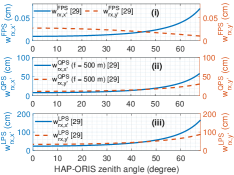
(a)

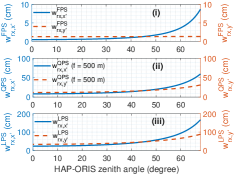
(b)

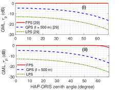
(c)

Figure 3: (a) Rx beam widths $w_{\text{rx},x^{\prime}}$ and $w_{\text{rx},y^{\prime}}$ versus zenith angle $\varphi_{\text{i}}$ for FPS (i), QPS (ii) and LPS (iii) profiles [29] ; (b) Rx beam widths $w_{\text{rx},x^{\prime}}$ and $w_{\text{rx},y^{\prime}}$ versus zenith angle $\varphi_{\text{i}}$ using the framework in this paper for FPS (i), QPS (ii) and LPS (iii) profiles; (c) Comparison of GML $\tau_{\text{p}}$ using the framework in [29] (i) versus that in this paper (ii) in the absence of PE.

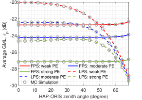
Figure 4: Average GML $\tau_{\text{p}}$ for FPS and LPS profiles under various PE severities induced by drone hovering fluctuations.

To highlight the atmospheric effects on the optical beam footprint, we compare the Rx beam widths at the drone for different ORIS phase-shift profiles using the frameworks developed in [29] and in this paper, as shown in Figs. 3a and 3b, respectively. It is observed in Fig. 3b(i) that atmospheric turbulence-induced beam broadening significantly affects the beam widths of the focused beam induced by the FPS profile. By contrast, this is ignored in Fig. 3a(i). Specifically, the beam broadening effect is most pronounced at the highest zenith angle of $\varphi_{\text{i}}\!=\!68^{\circ}$, due to the longest atmospheric path. The broadened beam resulting from turbulence is more than ten times larger than that caused by pure diffraction. On the other hand, for diffractive beams induced by the QPS and LPS profiles, the turbulence-induced beam broadening effect remains insignificant even at $\varphi_{\text{i}}\!=\!68^{\circ}$. For example, the broadening is only about 1 cm larger than that caused by pure diffraction, as shown in Figs. 3b(ii) and 3b(iii) compared to Figs. 3a(ii) and 3a(iii). Using the beam width values from Figs. 3a and 3b, we analyze the GML $\tau_{\text{p}}$ for all phase-shift profiles without PE based on the frameworks in [29] and this paper, as illustrated in Figs. 3c(i) and 3c(ii), respectively. As expected, the GML for the FPS profile under turbulence in Fig. 3c(ii) is not perfectly zero as in Fig. 3c(i), but it is significantly reduced to $-1.93$ dB at $\varphi_{\text{i}}=68^{\circ}$. Meanwhile, the GML values for the QPS and LPS profiles under turbulence in Fig. 3c(ii) remain approximately the same as in Fig. 3c(i), with only about a $0.1$ dB difference at $\varphi_{\text{i}}=68^{\circ}$.

It is evident from Fig. 3c(ii) that the FPS profile achieves the lowest GML, followed by the QPS and LPS profiles, in the absence of PE. This occurs because the GML is determined by the fraction of power captured by the Rx aperture, with smaller beams resulting in a higher fraction of received power. However, this trend does not hold for the average GML in the presence of PE induced by drone hovering fluctuations, as investigated in Fig. 4 for FPS and LPS profiles. Interestingly, the FPS profile results in higher average GML than the LPS profile for most paths for low zenith angles, such as $\varphi_{\text{i}}\!\leq\!49^{\circ},51^{\circ},61^{\circ}$ corresponding to weak, moderate, and strong PE conditions, respectively. This is because the random fluctuations in the drone’s position cause higher losses for smaller beam widths. However, at $\varphi_{\text{i}}\!>\!49^{\circ},51^{\circ},61^{\circ}$ for weak, moderate, and strong PE conditions, the average GML of the FPS profile surpasses that of the LPS profile. At high values of $\varphi_{\text{i}}$, the beam widths induced by the LPS profile become significantly broadened, resulting in higher geometrical loss. Finally, the accuracy of analytical results is validated through MC simulations, showing excellent agreement.

Following Fig. 4, we continue investigating the impact of PE on the average GML of the QPS profile under weak, moderate, and strong PE conditions in Figs. 5a, 5b, and 5c, respectively. The QPS profile represents an adaptive scheme capable of adjusting the beam widths, encompassing the FPS and LPS as special cases, when the focus distance parameter $f$ is set to infinity and $d_{2}/2$, respectively. The yellow regions in Figs. 5a, 5b, and 5c highlight the optimal values for the parameter $f$ to achieve the lowest average GML with respect to the zenith angle $\varphi_{\text{i}}$, where the minimum value of $f\!=\!d_{2}/2\!\cong\!176.77$ m corresponds to the special case of using the LPS profile. The LPS profile achieves the highest SKRs at small zenith angles, such as $\varphi_{\text{i}}\!\leq\!28^{\circ}$ and $\varphi_{\text{i}}\!\leq\!41^{\circ}$ in Figs. 5b and 5c, respectively, as a benefit of handling moderate-to-strong PE conditions, thanks to the wider beams. By contrast, the QPS profile optimizes the beam width by gradually increasing $f$, thereby narrowing the beam to an optimal size that effectively compensates for drone hovering fluctuations. This optimization is suitable for achieving the lowest GML over all zenith angles under weak PE conditions, as seen in Fig. 5a, while maintaining a consistent GML over high zenith angles, e.g., $\varphi_{\text{i}}\!>\!28^{\circ}$ and $\varphi_{\text{i}}\!>\!41^{\circ}$ for moderate and strong PE conditions in Figs. 5b and 5c, respectively.

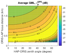
(a)

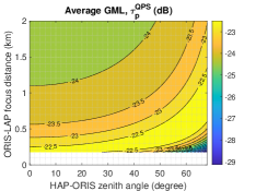
(b)

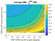
(c)

Figure 5: Average GML $\tau_{\text{p}}$ for the QPS profile under various PE severities induced by drone hovering fluctuations. (a) weak PE; (b) moderate PE; (c) strong PE.

V-B Average PLOB Bound of The SKR $\mathfrak{R}$

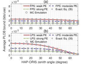
Figure 6: Average PLOB bound of the SKR $\mathfrak{R}$ (bits/use) under various PE severities induced by drone hovering fluctuations. (a) FPS profile; (b) LPS profile. The Laguerre polynomial order $G\!=\!180$.

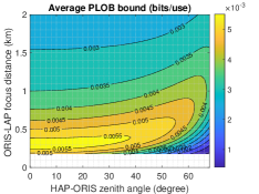
(a)

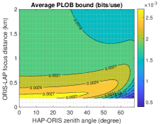
(b)

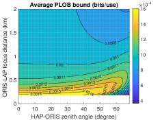
(c)

Figure 7: Average PLOB bound of the SKR $\mathfrak{R}$ (bits/use) for the QPS profile under various PE severities induced by drone hovering fluctuations. (a) weak PE; (b) moderate PE; (c) strong PE. The Laguerre polynomial order $G\!=\!180$.

In Fig. 6, we examine the average PLOB bound of the SKR $\mathfrak{R}$ for FPS (Fig. 6a) and LPS (Fig. 6b) profiles versus the PE levels. The analytical PLOB results, derived from Corollary 1, are corroborated by the exact form in (35) and validated through MC simulations, demonstrating excellent agreement. In accordance with the average GML $\tau_{\text{p}}$ results seen in Fig. 4, the LPS profile achieves higher SKRs for most paths over low zenith angles (e.g., $\varphi_{\text{i}}\!\leq\!49^{\circ},51^{\circ},61^{\circ}$), respectively under weak, moderate, and strong PE conditions, due to the lower average GML of the diverged beam that compensates for hovering fluctuations. By contrast, at $\varphi_{\text{i}}\!>\!49^{\circ},51^{\circ},61^{\circ}$ under weak, moderate, and strong PE conditions, the SKRs of the LPS profile decrease abruptly, as the beam widths become significantly broadened over longer distances, resulting in excessive losses. Conversely, although the beam widths induced by the FPS profile are further broadened at high values of $\varphi_{\text{i}}$, they remain considerably smaller than those of the LPS profile, helping to maintain the SKRs at higher values.

Eventually, the PLOB bound of the SKR $\mathfrak{R}$ found for the QPS profile is analyzed under weak, moderate, and strong PE conditions, as shown in Figs. 7a, 7b, and 7c, respectively. The yellow regions in Figs. 7a, 7b, and 7c indicate the optimal values for the parameter $f$ to achieve the highest average SKR relative to the zenith angle $\varphi_{\text{i}}$. Again, the minimum value of $f\!=\!d_{2}/2\!\cong\!176.77$ m corresponds to the special case of using the LPS profile. Similar to the observations in Fig. 5, the LPS profile is beneficial for compensating moderate-to-strong PE conditions due to its wider beams at small zenith angles, such as $\varphi_{\text{i}}\!\leq\!22^{\circ}$ and $\varphi_{\text{i}}\!\leq\!40^{\circ}$ in Figs. 7b and 7c, respectively. These optimal ranges found for the LPS profiles are lower than those in Figs. 5b and 5c, respectively, due to additional losses from $\tau_{\text{l}}$ at higher zenith angles, hence prompting the ORIS to use the QPS profile to achieve higher SKRs. As expected, the QPS profile configures the beam for an optimal size by gradually increasing $f$, which effectively mitigates the drone hovering fluctuations. This beam width optimization is effective in attaining the maximum SKRs across all zenith angles under weak PE conditions, as shown in Fig. 7a. It also maintains the highest possible SKRs at high zenith angles, such as $\varphi_{\text{i}}\!>\!22^{\circ}$ and $\varphi_{\text{i}}\!>\!40^{\circ}$, under moderate and strong PE conditions, as illustrated in Figs. 7b and 7c, respectively. Further increasing $f\!\rightarrow\!\infty$ would reduce the SKR to the level attained by the FPS profile in Fig. 6a.

VI Conclusions

The ORIS concept was developed for enhancing QKD links between HAPs and LAPs while mitigating the LAP’s hovering fluctuations. By reflecting HAP’s incoming beam via a rooftop-mounted ORIS to the terminal beneath the LAP, we established an efficient QKD link. An ORIS facilitates adaptive beam width control through LPS, QPS, and FPS profiles, optimizing the GML at the receiver. This necessitates a robust theoretical framework for accurately characterizing the ORIS-controlled optical beam propagation over atmospheric channels. We employ the EHF principles for the first time to precisely model the atmospheric turbulence effects imposed on ORIS-controlled beams. Our analytical model incorporates the LAP hovering fluctuations, offering a comprehensive framework for ORIS-aided non-terrestrial FSO systems. Utilizing this model, we derive the ultimate PLOB bound for the SKR of QKD protocols over HAP-ORIS-LAP links. Our findings demonstrate that the QPS profile optimizes the SKR at high zenith angles or under mild PE conditions by narrowing the beam to optimal sizes, while the LPS profile is advantageous at low zenith angles for the moderate-to-strong PE by diverging the beam to compensate for LAP fluctuations. These results underscore the efficiency of ORIS in mitigating PEs and optimizing the SKR across diverse operational conditions.

Appendix A Proof of Lemma 1

Following the framework in [29], with the help of [29, (54)], the statistical average GML coefficient $\tau_{\text{p}}$ in (30) can be approximated by $\tau_{\text{p}}^{\text{LPS}}$, for an LPS profile considering drone hovering fluctuations, written as

$$\tau_{\text{p}}^{\text{LPS}}\!\!= C_{\text{LPS}}\!\!\iint_{\!-\frac{a\sqrt{\pi}}{2}}^{\frac{a\sqrt{\pi}}{2}}\!\!\iint_{\!-\infty}^{\infty}\!\exp\!\!\left(\!\!-\frac{k^{2}\!\sin^{2}\!\!\left(\theta_{\text{r}}\right)\!\left(x^{\prime}\!+\!\tilde{x}^{\prime}\right)^{\!2}\!\mathcal{R}\!\left\{b_{x^{\prime}\!,\text{LPS}}\right\}}{2d_{2}^{2}\left|b_{x^{\prime}\!,\text{LPS}}\right|^{2}}\!\!\right)$$

$$\!\!\!\times\!\!\exp\!\!\left(\!\!-\frac{k^{2}\!\left(y^{\prime}\!+\!\tilde{y}^{\prime}\right)^{\!2}\!\mathcal{R}\!\left\{b_{y^{\prime}\!,\text{LPS}}\right\}}{2d_{2}^{2}\left|b_{y^{\prime}\!,\text{LPS}}\right|^{2}}\!\!\right)\!\!f_{\tilde{x}^{\prime}}\!\!\left(\tilde{x}^{\prime}\right)\!f_{\tilde{y}^{\prime}}\!\!\left(\tilde{y}^{\prime}\right)\!\text{d}x^{\prime}\!\text{d}y^{\prime}\!\text{d}\tilde{x}^{\prime}\!\text{d}\tilde{y}^{\prime}\!,$$ (37)

where $x^{\prime},y^{\prime}\!\in\!\left[-\frac{a\sqrt{\pi}}{2},\frac{a\sqrt{\pi}}{2}\right]$ and $\tilde{x}^{\prime},\tilde{y}^{\prime}\!\in\!\left(-\infty,\infty\right)$. Furthermore, we have $C_{\text{LPS}}\!=\!\frac{2P_{\text{t}}\sin\left(\theta_{\text{i}}\right)\!\sin\left(\theta_{\text{r}}\right)\pi}{\lambda^{2}w^{2}\!\left(d_{1}\right)d_{2}^{2}\left|b_{x^{\prime},\text{LPS}}\right|\left|b_{y^{\prime},\text{LPS}}\right|}$ with $b_{x^{\prime},\text{LPS}}\!=\!\frac{\sin^{2}\left(\theta_{\text{i}}\right)}{w^{2}\!\left(d_{1}\right)}\!+\!\frac{jk\sin^{2}\left(\theta_{\text{i}}\right)}{2R\left(d_{1}\right)}\!+\!\frac{jk\sin^{2}\left(\theta_{\text{r}}\right)}{2d_{2}}$ and $b_{y^{\prime},\text{LPS}}\!=\!\frac{1}{w^{2}\!\left(d_{1}\right)}\!+\!\frac{jk}{2R\left(d_{1}\right)}\!+\!\frac{jk}{2d_{2}}$. $f_{\tilde{x}^{\prime}}\!\!\left(\tilde{x}^{\prime}\right)$ and $f_{\tilde{y}^{\prime}}\!\!\left(\tilde{y}^{\prime}\right)$ are the Gaussian probability density functions (PDFs) of the hovering fluctuations $\tilde{x}^{\prime}$ and $\tilde{y}^{\prime}$, respectively, given by

$$f_{\nu}\!\!\left(\nu\right)\!=\!\frac{1}{\sqrt{2\pi\sigma_{\nu}^{2}}}\exp\!\left(-\frac{\left(\nu-\mu_{\nu}\right)^{2}}{2\sigma_{\nu}^{2}}\right),~{}\nu=\left\{\tilde{x}^{\prime},\tilde{y}^{\prime}\right\}.$$ (38)

Using [49, (4.3.13)] along with a change of variables, we arrive at the following result

$$\int_{-\infty}^{\infty}\!\!\text{erf}\!\left(\alpha\nu\!+\!\beta\right)\!\!\frac{\exp\!\!\left(\!-\frac{\left(\nu-\mu_{\nu}\right)^{2}}{2\sigma_{\nu}^{2}}\!\right)}{\sqrt{2\pi\sigma_{\nu}^{2}}}\text{d}\nu\!=\!\text{erf}\!\left(\!\!\frac{\alpha\mu_{\nu}\!+\!\beta}{\sqrt{1\!+\!2\alpha^{2}\sigma_{\nu}^{2}}}\!\right)\!\!.$$ (39)

By invoking (39) and [50, (2.33.1)], (A) can be solved and a closed-form expression is obtained in (31), where $w_{\text{rx},x^{\prime}}^{\text{LPS}}\!\!=\!\!w\!\left(d_{1}\right)\!\frac{\left|\sin\left(\theta_{\text{r}}\right)\right|}{\left|\sin\left(\theta_{\text{i}}\right)\right|}\sqrt{\!\varepsilon\!\left(\!\frac{\sin^{2}\left(\theta_{\text{i}}\right)}{\sin^{2}\left(\theta_{\text{r}}\right)}\Lambda_{1}\!\right)^{\!2}\!+\!\left(\!\frac{\sin^{2}\left(\theta_{\text{i}}\right)}{\sin^{2}\left(\theta_{\text{r}}\right)}\Lambda_{2}\!+\!1\!\right)^{\!2}}$ and $w_{\text{rx},y^{\prime}}^{\text{LPS}}\!=\!w\!\left(d_{1}\right)\!\sqrt{\varepsilon\Lambda_{1}^{2}\!+\!\left(\Lambda_{2}\!+\!1\right)^{2}}$ are the equivalent beam widths induced by the LPS profile at the Rx aperture in the $x^{\prime}$ and $y^{\prime}$ axes, respectively. Furthermore, $\Lambda_{1}\!=\!\frac{2d_{2}}{kw^{2}(d_{1})}$ and $\Lambda_{2}\!=\!\frac{d_{2}}{R(d_{1})}$ characterize the diffraction and refraction effects, respectively. Since $d_{1}\gg z_{\text{R1}}$, we have $R(d_{1})\!=\!d_{1}\!\left[1\!+\!\frac{z_{\text{R1}}}{d_{1}}\right]\!\approx\!d_{1}$, thus $\Lambda_{2}\!=\!\frac{d_{2}}{d_{1}}$. As $d_{1}\gg d_{2}$, $\Lambda_{2}\rightarrow 0$ and can be omitted, which gives the results of $w_{\text{rx},x^{\prime}}^{\text{LPS}}$ and $w_{\text{rx},y^{\prime}}^{\text{LPS}}$ in Lemma 1. This completes the proof.

Appendix B Proof of Lemma 2

Following the framework in [29], with the help of [29, (55)], the statistical average GML coefficient $\tau_{\text{p}}$ in (30) derived for a QPS profile by considering the drone hovering fluctuations can be approximated by $\tau_{\text{p}}^{\text{QPS}}$ as

$$\tau_{\text{p}}^{\text{QPS}}\!\!= C_{\text{QPS}}\!\!\iint_{\!-\frac{a\sqrt{\pi}}{2}}^{\frac{a\sqrt{\pi}}{2}}\!\!\iint_{\!-\infty}^{\infty}\!\!\exp\!\!\left(\!\!-\frac{k^{2}\!\sin^{2}\!\!\left(\theta_{\text{r}}\right)\!\left(x^{\prime}\!+\!\tilde{x}^{\prime}\right)^{\!2}\!\mathcal{R}\!\left\{b_{x^{\prime}\!,\text{QPS}}\right\}}{2d_{2}^{2}\left|b_{x^{\prime}\!,\text{QPS}}\right|^{2}}\!\!\right)$$

$$\!\!\!\!\times\!\!\exp\!\!\left(\!\!-\frac{k^{2}\!\left(y^{\prime}\!+\!\tilde{y}^{\prime}\right)^{\!2}\!\mathcal{R}\!\left\{b_{y^{\prime}\!,\text{QPS}}\right\}}{2d_{2}^{2}\left|b_{y^{\prime}\!,\text{QPS}}\right|^{2}}\!\!\right)\!\!f_{\tilde{x}^{\prime}}\!\!\left(\tilde{x}^{\prime}\right)\!f_{\tilde{y}^{\prime}}\!\!\left(\tilde{y}^{\prime}\right)\!\text{d}x^{\prime}\!\text{d}y^{\prime}\!\text{d}\tilde{x}^{\prime}\!\text{d}\tilde{y}^{\prime}\!,$$ (40)

where we have $C_{\text{QPS}}\!=\!\frac{2P_{\text{t}}\sin\left(\theta_{\text{i}}\right)\!\sin\left(\theta_{\text{r}}\right)\pi}{\lambda^{2}w^{2}\!\left(d_{1}\right)d_{2}^{2}\left|b_{x^{\prime},\text{QPS}}\right|\left|b_{y^{\prime},\text{QPS}}\right|}$ with $b_{x^{\prime},\text{QPS}}\!=\!\frac{\sin^{2}\left(\theta_{\text{i}}\right)}{w^{2}\!\left(d_{1}\right)}\!+\!\frac{jk\sin^{2}\left(\theta_{\text{r}}\right)}{4f}$ and $b_{y^{\prime},\text{QPS}}\!=\!\frac{1}{w^{2}\!\left(d_{1}\right)}\!+\!\frac{jk}{4f}$. Similar to Appendix A, by invoking (39) and [50, (2.33.1)], (B) can be solved and a closed-form expression is obtained in (32). This completes the proof.

Appendix C Proof of Lemma 3

Following the framework in [29], with the help of [29, (56)], the statistical average GML coefficient $\tau_{\text{p}}$ in (30) can be approximated by $\tau_{\text{p}}^{\text{FPS}}$ for an FPS profile considering drone hovering fluctuations as

$$\tau_{\text{p}}^{\text{FPS}}\!\!=C_{\text{FPS}}\!\!\iint_{-\frac{a\sqrt{\pi}}{2}}^{\frac{a\sqrt{\pi}}{2}}\!\!\iint_{-\infty}^{\infty} \!\exp\!\!\left(\!\!-\frac{2\!\left(x^{\prime}\!+\!\tilde{x}^{\prime}\right)^{\!2}}{\left(\!w_{\text{rx},x^{\prime}}^{\text{FPS}}\!\right)^{\!2}}-\frac{2\!\left(y^{\prime}\!+\!\tilde{y}^{\prime}\right)^{\!2}}{\left(\!w_{\text{rx},y^{\prime}}^{\text{FPS}}\!\right)^{\!2}}\!\!\right)$$

$$\!\times\!f_{\tilde{x}^{\prime}}\!\!\left(\tilde{x}^{\prime}\right)\!f_{\tilde{y}^{\prime}}\!\!\left(\tilde{y}^{\prime}\right)\!\text{d}x^{\prime}\!\text{d}y^{\prime}\!\text{d}\tilde{x}^{\prime}\!\text{d}\tilde{y}^{\prime}\!,$$ (41)

where $C_{\text{FPS}}\!=\!\frac{2P_{\text{t}}\pi w^{2}\!\left(d_{1}\right)\sin\left(\theta_{\text{r}}\right)}{\lambda^{2}d_{2}^{2}\sin\left(\theta_{\text{i}}\right)}$, $w_{\text{rx},x^{\prime}}^{\text{FPS}}\!=\!w\!\left(d_{1}\right)\!\frac{\left|\sin\left(\theta_{\text{i}}\right)\right|}{\left|\sin\left(\theta_{\text{r}}\right)\right|}\sqrt{\varepsilon\Lambda_{1}^{2}}$ and $w_{\text{rx},y^{\prime}}^{\text{FPS}}\!=\!w\!\left(d_{1}\right)\!\sqrt{\varepsilon\Lambda_{1}^{2}}$ are the equivalent beam widths induced by the FPS profile at the Rx aperture in the $x^{\prime}$ and $y^{\prime}$ axes, respectively. Similar to Appendix A, by invoking (39) and [50, (2.33.1)], (C) can be solved and a closed-form expression is obtained in (33). This completes the proof.

Appendix D Proof of Corollary 1

We have $I_{\text{a}}=I_{\text{a,1}}I_{\text{a,2}}$, where $I_{\text{a,1}}$ and $I_{\text{a,2}}$ are independent log-normal RVs, due to the distinct atmospheric paths of the HAP-ORIS and ORIS-drone links, respectively. Since $I_{\text{a,1}}\!\sim\!\mathcal{LN}(-\frac{\sigma_{\text{R},1}^{2}}{2},\sigma_{\text{R},1}^{2})$ and $I_{\text{a,1}}\!\sim\!\mathcal{LN}(-\frac{\sigma_{\text{R},1}^{2}}{2},\sigma_{\text{R},1}^{2})$, it is straightforward to obtain that $I_{\text{a}}\!\sim\!\mathcal{LN}(-\frac{\sigma_{\text{R},1}^{2}}{2}\!-\!\frac{\sigma_{\text{R},2}^{2}}{2},\sigma_{\text{R},1}^{2}\!+\!\sigma_{\text{R},2}^{2})$, where $\sigma_{\text{R},1}^{2}$ and $\sigma_{\text{R},2}^{2}$ are defined in (14). As a result, the term $f\!\left(I_{\text{a},1}\right)\!f\!\left(I_{\text{a},2}\right)$ in (35) can be replaced by $f\!\left(I_{\text{a}}\right)$, expressed as

$$f\!\left(I_{\text{a}}\right)\!=\!\frac{1}{I_{\text{a}}\sqrt{2\pi\sigma_{\text{R}}^{2}}}\exp\!\!\left(\!-\frac{\left(\ln\left(I_{\text{a}}\right)+\frac{\sigma_{\text{R}}^{2}}{2}\right)^{2}}{2\sigma_{\text{R}}^{2}}\!\right),$$ (42)

where $\sigma_{\text{R}}^{2}\!=\!\sigma_{\text{R},1}^{2}\!+\!\sigma_{\text{R}_{2}}^{2}$. Additionally, as $\tau$ is truncated at 1 to preserve the canonical commutation of the input-output quantum relationship, $I_{\text{a}}$ is restricted to $\left[0,1/\tau_{\text{eff}}\tau_{\text{l}}\tau_{\text{p}}\right]$, as seen in (35). However, due to the small values of $\tau_{\text{eff}}\tau_{\text{l}}\tau_{\text{p}}$, we can assume that $I_{\text{a}}\in\left[0,\infty\right)$, while satisfying the canonical commutation relationship via $\mathbb{E}\left[I_{\text{a}}\right]\!=\!1$ [47]. Subsequently, applying the identity of the Gauss-Laguerre quadrature $\int_{0}^{\infty}\!f\!\left(x\right)\text{d}x\!\cong\!\sum_{g=1}^{G}w_{g}e^{x_{g}}f\!\left(x_{g}\right)$ [52, Table 25.9], and with the help of Lemmas 1, 2, and 3, (35) can be derived as a closed-form expression in (36) for the FPS, QPS, and LPS profiles, respectively. This completes the proof.

References

- [1] Y. Cao , “The evolution of quantum key distribution networks: On the road to the qinternet,” IEEE Commun. Surveys Tuts., vol. 24, no. 2, pp. 839–894, 2nd Quart., 2022.
- [2] N. Hosseinidehaj , “Satellite-based continuous-variable quantum communications: State-of-the-art and a predictive outlook,” IEEE Commun. Surveys Tuts., vol. 21, no. 1, pp. 881–919, 1st Quart., 2019.
- [3] X. Liu, C. Xu, Y. Noori, S. X. Ng and L. Hanzo, “The road to near-capacity CV-QKD reconciliation: an FEC-agnostic design,” IEEE Open J. Commun. Soc., vol. 5, pp. 2089–2112, 2024.
- [4] P. V. Trinh , “Quantum key distribution over FSO: current development and future perspectives,” in Prog. Electromagn. Res. Symp. (PIERS-Toyama), 2018, pp. 1672–1679.
- [5] A. Carrasco-Casado , “LEO-to-ground polarization measurements aiming for space QKD using small optical transponder (SOTA),” Opt. Express, vol. 24, no. 11, pp. 12254–12266, 2016.
- [6] P. V. Trinh and S. Sugiura, “Quantum Internet in the sky: vision, challenges, solutions, and future directions,” IEEE Commun. Mag., in press.
- [7] G. Araniti, A. Iera, S. Pizzi, and F. Rinaldi, “Toward 6G non-terrestrial networks,” IEEE Netw., vol. 36, no. 1, pp. 113–120, Jan./Feb. 2022.
- [8] C.-Y. Lu, Y. Cao, C.-Z. Peng, and J.-W. Pan, “Micius quantum experiments in space,” Rev. Modern Phys., vol. 94, no. 3, Jul. 2022, Art. no. 035001.
- [9] Y. Chu, R. Donaldson, R. Kumar, and D. Grace, “Feasibility of quantum key distribution from high altitude platforms,” Quantum Sci. Technol., vol. 6, no. 3, p. 035009, 2021.
- [10] H.-Y. Liu , “Drone-based entanglement distribution towards mobile quantum networks,” Nat. Sci. Rev., vol. 7, no. 5, pp. 921–928, May 2020.
- [11] H.-Y. Liu , “Optical-relayed entanglement distribution using drones as mobile nodes,” Phys. Rev. Lett., vol. 126, no. 2, Jan. 2021, Art. no. 020503.
- [12] V. Jamali , “Intelligent reflecting surface assisted free-space optical communications,” IEEE Commun. Mag., vol. 59, no. 10, pp. 57–63, Oct. 2021.
- [13] H. Wang , “Optical reconfigurable intelligent surfaces aided optical wireless communications: opportunities, challenges, and trends,” IEEE Wirel. Commun., vol. 30, no. 5, pp. 28–35, Oct. 2023.
- [14] M. Najafi, B. Schmauss, and R. Schober, “Intelligent reflecting surfaces for free space optical communication systems,” IEEE Trans. Commun., vol. 69, no. 9, pp. 6134–6151, Sept. 2021.
- [15] A. R. Ndjiongue , “Analysis of RIS-based terrestrial-FSO link over G-G turbulence with distance and jitter ratios,” J. Lightw. Technol., vol. 39, no. 21, pp. 6746–6758, Nov. 2021.
- [16] H. Wang , “Approaches to array-type optical IRSs: schemes and comparative analysis,” J. Lightw. Technol., vol. 40, no. 12, pp. 3576–3591, Jun. 2022.
- [17] H. Wang , “Space division multiple access based on OIRS in multi-user FSO system,” IEEE Trans. Veh. Technol., vol. 71, no. 12, pp. 13403–13408, Dec. 2022.
- [18] H. Wang , “Performance analysis of hybrid RF-reconfigurable intelligent surfaces assisted FSO communication,” IEEE Trans. Veh. Technol., vol. 71, no. 12, pp. 13435–13440, Dec. 2022.
- [19] V. K. Chapala and S. M. Zafaruddin, “Unified performance analysis of reconfigurable intelligent surface empowered free-space optical communications,” IEEE Trans. Commun., vol. 70, no. 4, pp. 2575–2592, Apr. 2022.
- [20] J. -H. Noh and B. Lee, “Phase-shift design and channel modeling for focused beams in IRS-assisted FSO systems,” IEEE Trans. Veh. Technol., vol. 72, no. 8, pp. 10971–10976, Aug. 2023.
- [21] H. Wang , “Optical MIMO communication based on joint control of base station and OPA-type OIRS,” J. Lightw. Technol., vol. 41, no. 17, pp. 5546–5556, Sept. 2023.
- [22] H. Wang , “Optical intelligent reflecting surface for cascaded FSO-VLC communication system,” IEEE Trans. Veh. Technol., vol. 72, no. 10, pp. 13740–13745, Oct. 2023.
- [23] T. V. Nguyen, H. D. Le, and A. T. Pham, “On the design of RIS-UAV relay-assisted hybrid FSO/RF satellite-aerial-ground integrated network,” IEEE Trans. Aerosp. Electron. Syst., vol. 59, no. 2, pp. 757–771, Apr. 2023.
- [24] X. Li , “RIS assisted UAV for weather-dependent satellite terrestrial integrated network with hybrid FSO/RF systems,” IEEE Photonics J., vol. 15, no. 5, pp. 1–17, Oct. 2023, Art. no. 7304217.
- [25] Y. Ata, A. M. Vegni, and M. S. Alouini, “RIS-embedded UAVs communications for multi-hop fully-FSO backhaul links in 6G networks,” IEEE Trans. Veh. Technol. (Early Access), doi: 10.1109/TVT.2024.3414850.
- [26] T. Ishida, C. B. Naila, H. Okada, and M. Katayama, “Performance analysis of IRS-assisted multi-link FSO system under pointing errors,” IEEE Photonics J., vol. 16, no. 4, pp. 1–10, Aug. 2024, Art. no. 7302510.
- [27] H. Ajam , “Modeling and design of IRS-assisted multilink FSO systems,” IEEE Trans. Commun., vol. 70, no. 5, pp. 3333–3349, May 2022.
- [28] J. Sipani, P. Sharda, and M. R. Bhatnagar, “Modeling and design of IRS-assisted FSO system under random misalignment,” IEEE Photonics J., vol. 15, no. 4, pp. 1–13, Aug. 2023, Art. no. 7303113.
- [29] H. Ajam, M. Najafi, V. Jamali, and R. Schober, “Optical IRSs: power scaling law, optimal deployment, and comparison with relays,” IEEE Trans. Commun., vol. 72, no. 2, pp. 954–970, Feb. 2024.
- [30] S. Kisseleff and S. Chatzinotas, “Trusted reconfigurable intelligent surface for multi-user quantum key distribution,” IEEE Commun. Lett., vol. 27, no. 8, pp. 2237–2241, Aug. 2023.
- [31] N. K. Kundu, M. R. McKay, R. Murch, and R. K. Mallik, “Intelligent reflecting surface-assisted free space optical quantum communications,” IEEE Trans. Wirel. Commun., vol. 23, no. 5, pp. 5079–5093, May 2024.
- [32] A. E. Minovich , “Functional and nonlinear optical metasurfaces,” Laser Photon. Rev., vol. 9, no. 2, pp. 195–213, Mar. 2015.
- [33] L. C. Andrews and R. L. Phillips, Laser Beam Propagation Through Random Media. Bellingham, WA, USA: SPIE Press, 2005.
- [34] R. F. Lutomirski and H. T. Yura, “Propagation of a finite optical beam in an inhomogeneous medium,” Appl. Opt., vol. 10, no. 7, pp. 1652–1658, 1971.
- [35] J. C. Ricklin and F. M. Davidson, “Atmospheric turbulence effects on a partially coherent Gaussian beam: implications for free-space laser communication,” J. Opt. Soc. Am. A, vol. 19, no. 9, pp. 1794–1802, Sept. 2002.
- [36] P. V. Trinh , “Experimental channel statistics of drone-to-ground retro-reflected FSO links with fine-tracking systems,” IEEE Access, vol. 9, pp. 137148–137164, 2021.
- [37] A. Carrasco-Casado , “Development of a miniaturized lasercommunication terminal for small satellites,” Acta Astronaut., vol. 197, pp. 1–5, 2022.
- [38] D. R. Kolev , “Latest developments in the field of optical communications for small satellites and beyond,” J. Lightw. Technol., vol. 41, no. 12, pp. 3750–3757, Jun. 2023.
- [39] A. Carrasco-Casado , “Miniaturized multi-platform free-space laser-communication terminals for beyond-5G networks and space applications,” Photonics, vol. 11, no. 6, pp. 1–18, Jun. 2024, Art. no. 545.
- [40] Z. Ghassemlooy, W. Popoola, and S. Rajbhandari, Optical Wireless Communications: System and Channel Modelling With MATLAB. Boca Raton, FL, USA: CRC Press, 2012.
- [41] C. Weedbrook , “Gaussian quantum information,” Rev. Mod. Phys., vol. 84, no. 2, p. 621, May 2012.
- [42] A. A. Semenov and W. Vogel, “Quantum light in the turbulent atmosphere,” Phys. Rev. A, vol. 80, no. 2, 2009, Art. no. 021802(R).
- [43] R. J. Glauber, “Coherent and incoherent states of the radiation field,” Phys. Rev., vol. 131, no. 6, pp. 2766–2788, Sept. 1963.
- [44] E. C. G. Sudarshan, “Equivalence of semiclassical and quantum mechanical descriptions of statistical light beams,” Phys. Rev. Lett., vol. 10, no. 7, pp. 277–279, Apr. 1963.
- [45] D. Dequal , “Feasibility of satellite-to-ground continuous-variable quantum key distribution,” NPJ Quantum Inf., vol. 7, no. 1, pp. 1–10, Jan. 2021.
- [46] D. P. Greenwood, “Bandwidth specification for adaptive optics systems,” J. Opt. Soc. America, vol. 67, no. 3, pp. 390–393, 1977.
- [47] P. V. Trinh , “Statistical verifications and deep-learning predictions for satellite-to-ground quantum atmospheric channels,” Commun. Phys., vol. 5, pp. 1–18, Sept. 2022, Art. no. 225.
- [48] M. Ghalaii and S. Pirandola, “Quantum communications in a moderate-to-strong turbulent space,” Commun. Phys., vol. 5, pp. 1–12, Feb. 2022, Art. no. 38.
- [49] E. W. Ng and M. Geller, “A table of integrals of the error functions,” J. Res. Natianal Bureau Standards-B. Math. Sci., vol. 73B, no. 1, Jan./Mar. 1969.
- [50] I. S. Gradshteyn and I. M. Ryzhik, Table of Integrals, Series, and Products. 8th ed. San Diego, CA, USA: Academic, 2015.
- [51] S. Pirandola, R. Laurenza, C. Ottaviani, and L. Banchi, “Fundamental limits of repeaterless quantum communications,” Nature Commun., vol. 8, no. 1, p. 15043, Apr. 2017.
- [52] M. Abramowitz and I. A. Stegun, Handbook of Mathematical Functions: With Formulas, Graphs, and Mathematical Tables, 9th ed. New York, NY, USA: Dover, 1972.