Quantum synchronization between two spin chains using pseudo-bosonic equivalence

Abstract

Quantum synchronization among many spins is an intriguing domain of research. In this paper, we explore the quantum synchronization of two finite chains of spin-1/2 particles, via a nonlinear interaction mediated by a a central intermediary spin chain. We introduce a novel approach using the Holstein-Primakoff transformation to treat the spin chains as pseudo-bosonic systems and thereby applying the synchronization criteria for harmonic oscillators. Our theoretical framework and numerical simulations reveal that under optimal conditions, the spin chains can achieve both classical and perfect quantum synchronization. We show that quantum synchronization is robust against variations in the number of spins and inter-spin coupling, though may be affected by thermal noise. This work advances the understanding of synchronization in multi-spin systems and introduces a generalized synchronization measure for both bosons and fermions.

I INTRODUCTION

Recent advances in quantum synchronization, at the crossroads of quantum physics and nonlinear dynamics, offer an exciting domain of research pikovsky2001universal ; strogatz2018nonlinear ; huygens1897oeuvres . Usually, in the classical regime, one explores synchronized patterns in coupled oscillators huygens1897oeuvres , which persists even at different natural frequencies of these oscillators pikovsky2001universal ; strogatz2018nonlinear ; huygens1897oeuvres ; arenas2008synchronization . In the quantum regime, on the other hand, these studies can be extended to a few-level systems, leading to a more generalized approach to synchronization. Quantum synchronization has been studied in various platforms, e.g., van der Pol oscillators, Josephson junction arrays, spin torque nano-oscillators, and optomechanical systems heinrich2011collective ; holmes2012synchronization ; zhang2012synchronization ; PhysRevLett.111.103605 ; wiesenfeld1996synchronization ; kaka2005mutual ; shim2007synchronized ; shim2007synchronized ; manzano2013avoiding ; manzano2013synchronization ; giorgi2012quantum .

These studies hold significant promise for applications in quantum information processing, communication, and control. An interesting relation between quantum Fisher information and quantum synchronization has recently been outlined in vaidya2024quantumsynchronizationdissipativequantum , which makes synchronization relevant, even in the domain of quantum sensing.

While quantum synchronization is traditionally studied among two or more coupled oscillators, spin synchronization is comparably a newer concept. In this context, we note that quantum synchronization between two spatially separated spin-1/2 qubit clocks has been proposed in PhysRevLett.85.2006 ; PhysRevLett.85.2010 ; shi2022clock , which refers to adjusting their time-difference by taking advantage of entanglement shared between them. These ideas have been demonstrated using photons liu2021quantum ; refId0 and nuclear magnetic resonance PhysRevA.70.062322 . Multiparty clock synchronization has also been proposed PhysRevA.66.024305 ; PhysRevA.84.014301 ; PhysRevA.86.014301 and experimentally demonstrated kong2018demonstration . The effect of decoherence on such synchronization has been studied in noorbakhsh2024quantum . Clock synchronization without entanglement is also proposed in PhysRevA.72.042301 .

It is however shown that to synchronize a quantum system to an external driving, the relevant Hilbert space should have a minimum size of 3 PhysRevLett.121.053601 , as a single qubit cannot be entrained due to the lack of a limit cycle. There have been several reports of synchronizing a single qubit, e.g., when coupled to a driven dissipating oscillator PhysRevLett.100.014101 or via a mechanical resonator PhysRevA.107.013528 , or in a trapped ion PhysRevResearch.5.033209 . That a single qubit can be understood as containing a valid limit cycle has been discussed in PhysRevA.101.062104 . Synchronization of a single spin has further been demonstrated using Nitrogen-vacancy spin qubit in a radio-frequency field PhysRevLett.112.010502 and emulated in IBM Q system PhysRevResearch.2.023026 .

Quantum synchronization between two spins, on the other hand, is interpreted in terms of constant phase relations between the corresponding limit cycles or the relative phase of their respective Bloch vectors PhysRevA.94.032336 . It is shown that two qubits can be synchronized via their coupling to a common bath PhysRevA.88.042115 , or via a coherent coupling with each other, while each being coupled to a separate bath PhysRevA.109.033718 or due to collision PhysRevA.100.012133 , without any external driving or when coupled to a driven dissipative resonator PhysRevB.80.014519 . Phase synchronization of two nuclear spins has been experimentally verified in terms of Husimi Q-function PhysRevA.105.062206 .

Two-spin synchronization has also been described as a persistent oscillation of the eigenmodes of the corresponding Liouvillean in the presence of decay. This idea was demonstrated in a system of three spins, the Hamiltonian of which conserves total magnetization 10.21468/SciPostPhys.12.3.097 . Two spins of this trio exhibit antisynchronization in the transverse components of the local spins buvca2022algebraic , thanks to the inherent dynamical and permutation symmetry. Note that such synchronization between two qubits has been explored via their common coupling with a third qubit. The mediated synchronization between two qubits has also been explored in an ion trap in the presence of a damped normal mode of the collective vibration of the ions PhysRevA.95.033423 .

While there have been several studies of quantum synchronization of a single qubit and two qubits, there has been very little investigation on many-qubit synchronization. Li et al. investigated synchronization in a few-spins system with non-local dissipation, revealing stable oscillatory behaviors in long-time dynamics without external driving PhysRevA.107.032219 . Stable (anti)synchronization between local spin observables can be induced by noise, under specific conditions in an isolated quantum many-body system goldobin2005synchronization ; schmolke2022noise . A generalized concept of synchronization, namely, measure synchronization has been introduced PhysRevA.90.033603 to study the coordinated dynamics of two many-body systems, coupled via contact particle-particle interactions. Correlated phase dynamics of two mesoscopic ensembles of atoms also exhibit synchronization, via their common coupling to an optical cavity PhysRevLett.113.154101 .

In this paper, we demonstrate how two long chains of spin-1/2 particles can be quantum synchronized. A spin chain is essentially a one-dimensional (1D) lattice, with distance-dependent exchange interactions between any two spins. We consider only the nearest neighborhood interactions, as in usual 1D Ising models. Such models have been previously studied for entanglement propagation and quantum phase transitions pappalardi2018scrambling ; abanin2019colloquium ; ramos2020optical . In our case, these two chains interact nonlinearly via their common coupling to another intermediary spin-chain. In the previous works, spin synchronization has been characterized in terms of either Husimi Q-function PhysRevA.105.062206 ; PhysRevLett.121.053601 ; PhysRevLett.121.063601 ; PhysRevA.101.062104 ; PhysRevResearch.5.033209 ; PhysRevA.109.033718 or Pearson spin-spin correlation function PhysRevA.100.012133 . We employ a different approach - we treat the spin chain as a pseudo-bosonic system. We introduce an equivalent pseudo-bosonic operator for the collective spin of the finite-size chain using the Holstein-Primakoff transformation PhysRev.58.1098 . This enables us to use the standardized criterion of quantum synchronization of two harmonic oscillators PhysRevLett.111.103605 . Note that the transformation ‘from-spin-to-boson’ explicitly reveals the inherent nonlinearity in the system which leads to the synchronization. It is anticipated that quantum synchronization is a certain manifestation of quantum correlations. In fact the criterion used in PhysRevLett.111.103605 originates from the Heisenberg uncertainty principle, in the context of EPR-like variables garg2023quantum ; dasgupta2023entanglement .

The paper proceeds as follows. In Section II, we introduce the model, including its mean field approximation and necessary dynamical equations. We discuss the main results of synchronization in terms of the limit cycles and synchronization markers, in Section III. We conclude the paper in Section IV.

II MODEL AND EQUATION OF MOTION

We will study synchronization between two distinct finite spin chains, consisting of $N_{1}$ and $N_{2}$ spin-1/2 particles [each depicted as red dots in Fig. 1(a)], respectively. These chains are weakly coupled to a common spin chain [the spins of which are depicted as black dots in Fig. 1(a)], via the site-specific spin-spin coupling (coupling constant $g_{j}$, $j\in 1,2$). This central chain acts as an intermediary to build up synchronization between two other chains. We further assume a nearest-neighbour coupling between the spins, with a coupling constant $\lambda^{2}\omega_{j}$ ($j\in 1,2$), where $\omega_{j}$ is the frequency of each spin in the $j$th chain and $0\leq\lambda\leq 1$ is a weight factor. Here $\lambda\sim 0$ ($\lambda\lesssim 1$) refers to weak (strong) coupling among the spins.

For an odd number of spins, the intermediary chain exhibits a ground state doublet. At low temperatures, this chain is assumed to remain confined to this doublet and hence may be considered as an equivalent single spin [depicted by a black circle in Fig. 1(b)]. The coupling between two chains is now essentially mediated via this single spin, with a coupling constant modified by a factor of $1/\sqrt{N_{j}}$. The equivalent Hamiltonian is then expressed as follows:

$$H=H_{S}+\sum_{j=1}^{2}(H_{SB_{j}}+H_{B_{j}})\;,$$ (1)

where

$$H_{S} = \frac{\hbar\omega_{0}}{2}\sigma_{z}^{0}\;,$$

$$H_{SB_{j}} = \frac{\hbar g_{j}}{2\sqrt{N_{j}}}\sum_{i=1}^{N_{j}}\left(\sigma_{x}^{0}\sigma_{jx}^{i}+\sigma_{y}^{0}\sigma_{jy}^{i}+\sigma_{z}^{0}\sigma_{jz}^{i}\right)\;,$$

$$H_{B_{j}} = \frac{\hbar\omega_{j}}{2N_{j}}\sum_{i=1}^{N_{j}}\left\{\frac{1}{2}\sum_{\begin{subarray}{c}k=1\\ k\neq i\end{subarray}}^{N_{j}}\left[\lambda^{2}(\sigma_{jx}^{i}\sigma_{jx}^{k}+\sigma_{jy}^{i}\sigma_{jy}^{k})\right]+\sigma_{jz}^{i}\right\}\;.$$ (2)

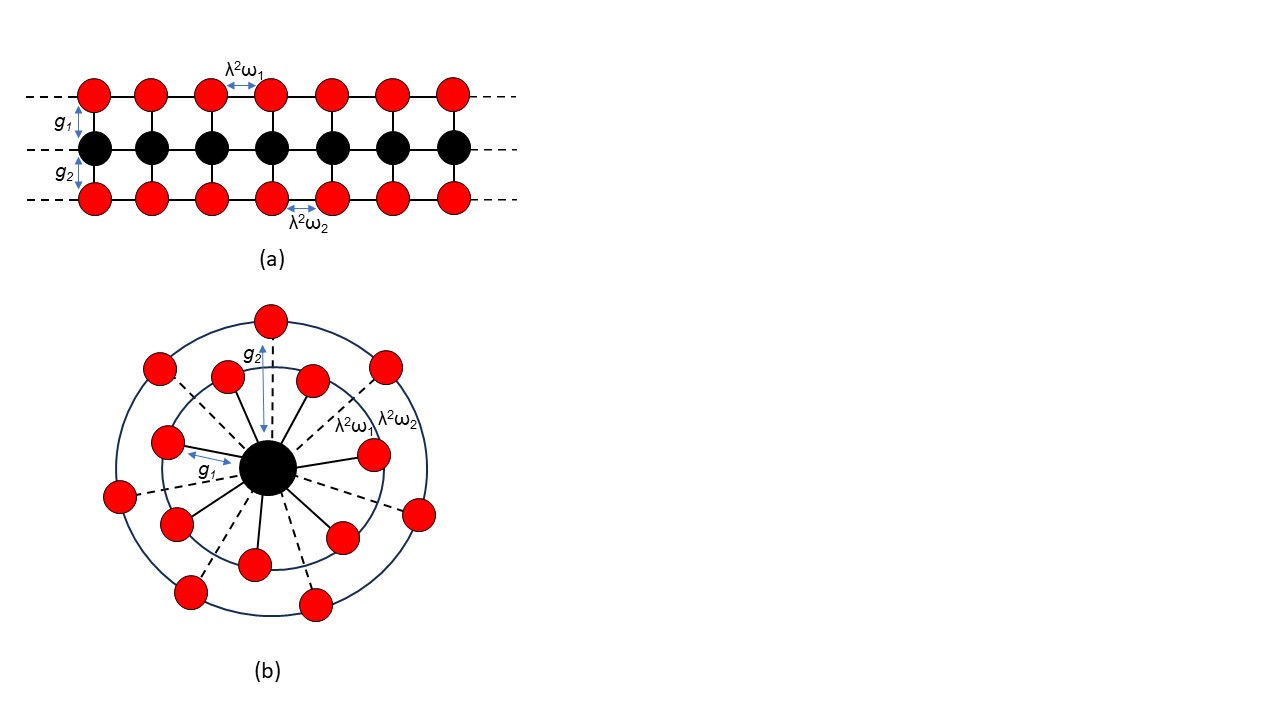
Figure 1: Schematic of a generic (a) Spin Chain Model, (b) Central-Spin Model

Next, we invoke the collective spin angular momentum operator, $J_{jk^{\prime}}=\frac{1}{2}\sum_{i=1}^{N_{j}}\sigma_{jk^{\prime}}^{i}$ (where $k^{\prime}\in\{\text{x},\text{y},\text{z},+,-\}$ and $j\in\{1,2\}$). Then the different parts of $H$ can be rewritten as

$$H_{SB_{j}} = \frac{\hbar g_{j}}{\sqrt{N_{j}}}\left(\sigma_{x}^{0}J_{jx}+\sigma_{y}^{0}J_{jy}+\sigma_{z}^{0}J_{jz}\right)\;,$$

$$H_{B_{j}} = \hbar\omega_{j}\left[\lambda^{2}\left(\frac{J_{j+}J_{j-}}{N_{j}}-\frac{\mathbb{1}}{2}\right)+(1-\lambda^{2})\frac{J_{jz}}{N_{j}}\right]\;$$ (3)

Note that the Hamiltonian $H_{SB_{j}}$ can be rewritten as $\frac{\hbar g_{j}}{\sqrt{N_{j}}}\vec{\sigma^{0}}.\vec{J_{j}}$, which represents an effective coupling between the central spin and the collective spin. For brevity, we will replace $\sigma^{0}$ with $\sigma$.

As we mentioned in the Introduction, we will analyze spin synchronization in terms of bosons. In this regard, we introduce bosonic operators using the Holstein-Primakoff (HP) transformation PhysRev.58.1098 ; PhysRevA.96.052125 ; PhysRevA.106.032435 :

$$J_{j+} = \sqrt{N_{j}}b_{j}^{\dagger}\left(1-\frac{b_{j}^{\dagger}b_{j}}{2N_{j}}\right)^{1/2}\;,$$

$$J_{j-} = J_{j+}^{\dagger}=\sqrt{N_{j}}\left(1-\frac{b_{j}^{\dagger}b_{j}}{2N_{j}}\right)^{1/2}b_{j}\;,$$

$$J_{jz} = b_{j}^{\dagger}b_{j}-N_{j}\;.$$ (4)

Then the Hamiltonian gets modified to ($\hbar=1$)

$$H_{SB_{j}} = g_{j}\left[\left\{\frac{\sigma_{+}}{2}\left(1-\frac{b_{j}^{\dagger}b_{j}}{4N_{j}}\right)b_{j}+{\rm h.c}\right\}+\frac{\sigma_{z}}{\sqrt{N_{j}}}\left(b_{j}^{\dagger}b_{j}-N_{j}\right)\right]\;,$$

$$H_{B_{j}} = {\omega_{j}}\left[b_{j}^{\dagger}b_{j}B_{j}-\lambda^{2}\frac{(b_{j}^{\dagger}b_{j})^{2}}{2N_{j}}+\left(\frac{\lambda^{2}}{2}-1\right)\mathbb{1}\right]\;,$$ (5)

where $B_{j}=\lambda^{2}\left(1-\frac{1}{2N_{j}}\right)+\frac{1}{N_{j}}$ for $j\in\{1,2\}$. Here, $b_{j}$ and $b_{j}^{\dagger}$ are the bosonic annihilation and creation operators with the property $\left[b_{j},b_{j}^{\dagger}\right]=1$. In the Hamiltonian $H_{SB_{j}}$ in Eq. (5), we have considered the terms up to the order of $1/N_{j}$, while expanding the series of $(1-b_{j}^{\dagger}b_{j}/2N_{j})^{1/2}$. Note that for an infinite spin chain $(N_{j}\rightarrow\infty)$, the above HP transformation makes a collective spin annihilation operator equivalent to a bosonic annihilation operator. In this paper, we are however focusing on finite spin chains.

Incorporating the interaction picture and using the Baker–Campbell–Hausdorff formalism, the refined Hamiltonian $H^{\prime}(t)$ can be expressed as $(\iota=\sqrt{-1})$

$$H^{\prime}(t) =\sum_{j=1}^{2}\left\{g_{j}\exp\left[\iota t\left(\omega_{0}-\omega_{j}B_{j}\right)\right]\sigma_{+}\left(1-\frac{b_{j}^{\dagger}b_{j}}{4N_{j}}\right)\right.$$ (6)

$$\left.\quad\times\exp\left[\iota\lambda^{2}\omega_{j}t\left(\frac{b_{j}^{\dagger}b_{j}+b_{j}b_{j}^{\dagger}}{2N_{j}}\right)\right]b_{j}+\text{h.c.}\right\}$$

$$\quad+g_{j}\frac{\sigma_{z}}{\sqrt{N_{j}}}\left(b_{j}^{\dagger}b_{j}-N_{j}\right)$$

We assume that the central spin mediates an indirect interaction between two spin chains. The transition probability between the two levels of the central spin is assumed to remain negligible at the time scale of the evolution of the spin chain operators $b_{j}$s, leading to the adiabatic elimination of the central spin operators. Consequently, the time derivatives of the raising and lowering operators $\dot{\sigma}_{\pm}$ are both zero. We thereby obtain the expression of $\sigma_{\pm}$, in which we replace $\sigma_{z}$ with its average value $\langle\sigma_{z}\rangle$. The Hamiltonian $H^{\prime}(t)$ thus takes the following form:

$$H^{\prime}(t)=\sum_{j=1}^{2}\frac{\langle\sigma_{z}\rangle}{X}g_{j}^{2}b_{j}^{\dagger}\left(1-\frac{b_{j}^{\dagger}b_{j}}{4N_{j}}\right)^{2}b_{j}+({P_{1}}{P_{2}^{\dagger}}+{\rm h.c.})+\langle\sigma_{z}\rangle\;,$$ (7)

where

$$P_{j} = g_{j}b_{j}^{\dagger}\exp\left[R_{j}\left(b_{j}^{\dagger}b_{j}+b_{j}b_{j}^{\dagger}\right)\right]\left(1-\frac{b_{j}^{\dagger}b_{j}}{4N_{j}}\right)\exp\left(-\iota\omega_{j}B_{j}t\right)\;,$$

$$R_{j} = \iota\omega_{j}\left(\frac{\lambda^{2}}{2N_{j}}\right)t\;,$$

$$X = \sum_{j=1}^{2}g_{j}\frac{1}{\sqrt{N_{j}}}\left(\langle b_{j}^{\dagger}b_{j}\rangle-N_{j}\right)\;.$$ (8)

Note that the above Hamiltonian is inherently nonlinear. Here we assumed $\langle\sigma_{z}\rangle$ to be constant.

We study the spin-chain synchronization in terms of that of the bosons $b_{j}$. This is the key difference between our approach and other relevant works. We first obtain Langevin’s equations for these annihilation operators, as presented in Appendix A. To obtain these equations (22) and (23), we used the transformations $b_{1}\to\widetilde{b_{1}}\exp(-\iota\theta t)$ and $b_{2}\to\widetilde{b_{2}}\exp(\iota\theta t)$ where $\theta=\left[\left(\frac{\omega_{2}}{2}\right)B_{2}-\left(\frac{\omega_{1}}{2}\right)B_{1}\right]$. For the sake of brevity, we will denote $\widetilde{b_{1}}$ and $\widetilde{b_{2}}$ by $b_{1}$ and $b_{2}$, respectively in the later sections. Further, $\gamma_{l}$ and $\gamma_{nl}$ are the linear and nonlinear dissipation rates of the system, respectively. Accordingly, the input noise operators ${b}_{in}^{(1)}$ and ${b}_{in}^{(2)}$ exhibit the following two-time correlation functions:

$$\left\langle\hat{b}_{\text{in}}^{(j)}(t)\hat{b}_{\text{in}}^{(j)\dagger}(t^{\prime})\right\rangle =\left(\bar{n}_{m}+1\right)\delta(t-t^{\prime})$$ (9)

$$\left\langle\hat{b}_{\text{in}}^{(j)\dagger}(t)\hat{b}_{\text{in}}^{(j)}(t^{\prime})\right\rangle =\bar{n}_{m}\delta(t-t^{\prime})\;.$$

Here $\bar{n}_{m}$ is the average phonon number of the thermal bath, common to both the spin chains.

II.1 Solution in mean-field approximation

Due to the analytical complexity of solving the equations (22) and (23), we employ the mean-field approximation to simplify calculations. In the limit of large excitation of the bosonic modes, the relevant operators can be expressed as the sum of their mean values and quantum fluctuations near the mean values, i.e., ${b}_{j}\rightarrow\left\langle{b}_{j}\right\rangle+\delta{b}_{j}={\beta}_{j}+\delta{b}_{j}$. The equations for these mean values $\beta_{j}$ are written in Appendix B. The Eqs. (24) and (25) would represent the independent damped oscillation of the two modes, if $\langle\sigma_{z}\rangle=0$, i.e., if the central spin is prepared in an equal superposition of its bare states, namely, $|0\rangle$ and $|1\rangle$. This would be the only possibility as the condition $\langle\sigma_{z}\rangle=0$ cannot be achieved in thermal equilibrium. Note that the states $|0\rangle$ and $|1\rangle$ are themselves many-spin states.

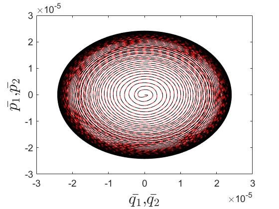
(a)

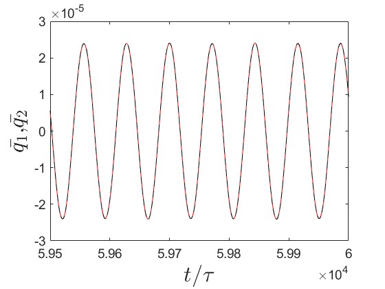
(b)

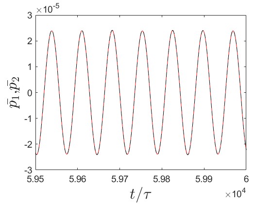
(c)

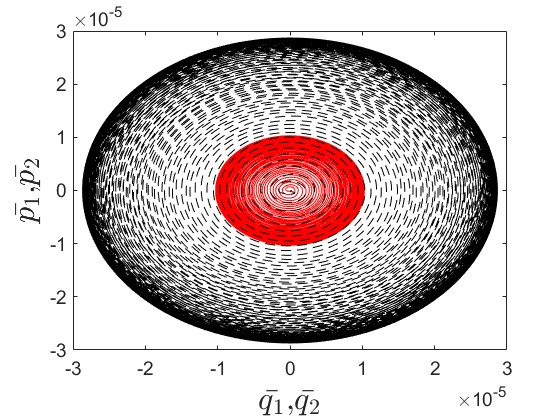
(d)

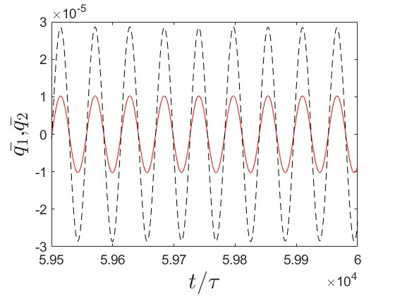
(e)

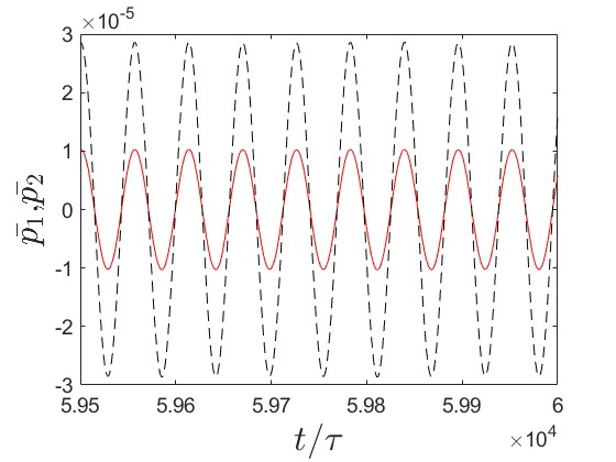
(f)

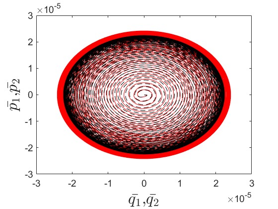
(g)

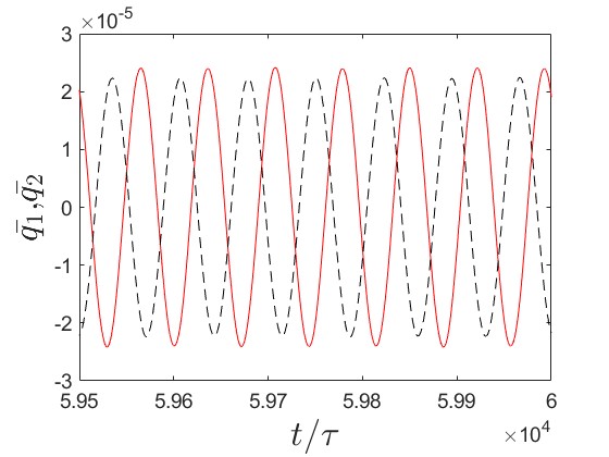
(h)

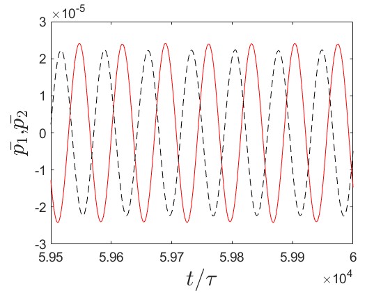
(i)

Figure 2: (a) Limit-cycle trajectories in the $\bar{q_{1}}\leftrightharpoons\bar{p_{1}}$ (red) and $\bar{q_{2}}\leftrightharpoons\bar{p_{2}}$ (black) spaces, (b) Variation of the mean values $\bar{q_{1}}$ (red) and $\bar{q_{2}}$ (black), (c) the mean values $\bar{p_{1}}$ (red) and $\bar{p_{2}}$ (black). The parameters chosen are $\lambda=0$, $N_{1}=N_{2}=5$.(d) Limit-cycle trajectories in the $\bar{q_{1}}\leftrightharpoons\bar{p_{1}}$ (red) and $\bar{q_{2}}\leftrightharpoons\bar{p_{2}}$ (black) spaces, (e) Variation of the mean values $\bar{q_{1}}$ (red) and $\bar{q_{2}}$ (black), (f) the mean values $\bar{p_{1}}$ (red) and $\bar{p_{2}}$ (black). The parameters chosen are $\lambda=0$, $N_{1}=10$, $N_{2}=5$. (g) Limit-cycle trajectories in the $\bar{q_{1}}\leftrightharpoons\bar{p_{1}}$ (red) and $\bar{q_{2}}\leftrightharpoons\bar{p_{2}}$ (black) spaces, (h) Variation of the mean values $\bar{q_{1}}$ (red) and $\bar{q_{2}}$ (black), (i) the mean values $\bar{p_{1}}$ (red) and $\bar{p_{2}}$ (black). The parameters chosen are $\lambda=0.2$, $N_{1}=N_{2}=5$ and $\phi=1.049$. All the other parameters are the same in all the above figures: $g_{1}=1.5$, $g_{2}=2.4$, $\langle\sigma_{z}\rangle=-0.1$, $\omega_{1}=1$, $\omega_{2}=0.8$,$\gamma_{l}=0.001$,$\gamma_{nl}=0.002$.

To calculate the desired marker $S_{q}$ for quantum synchronization, we need to solve for the quadrature fluctuations of the oscillators. Solving equations (22) and (23) becomes more convenient by replacing relevant operators and input noise operators with their quadratures: $\delta q_{j}=\frac{1}{\sqrt{2}}\left(\delta b^{\dagger}_{j}+\delta b_{j}\right)$, $\delta p_{j}=\frac{\iota}{\sqrt{2}}\left(\delta b^{\dagger}_{j}-\delta b_{j}\right)$, $q_{in}=\frac{1}{\sqrt{2}}\left(b_{in}^{\dagger}+b_{in}\right)$, and $p_{in}=\frac{\iota}{\sqrt{2}}\left(b_{in}^{\dagger}-b_{in}\right)$. In the limit of negligible higher order fluctuations, we obtain the Eqs. (C) which are linearized equations for the quantum fluctuations. We have included the exact forms of these equations in Appendix C.

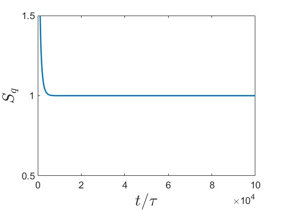
(a)

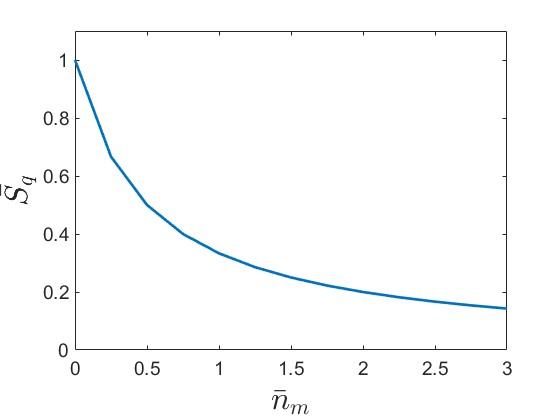
(b)

Figure 3: Variation of $S_{q}$, with respect to (a) time $t$ (in the units of $\tau=1/\omega_{1}$) and Variation of $\bar{S}_{q}$,with respect to (b) the mean phonon number $\bar{n}_{m}$ of the environment. The other parameters are $g_{1}=1.5$, $g_{2}=2.4$ , $\langle\sigma_{z}\rangle=-0.1$, $\omega_{1}=1$, $\omega_{2}=0.8$, $\gamma_{l}=0.001$, $\gamma_{nl}=0.002$, $\phi=1.049$.

Therefore, the fluctuation equations take a simpler form as given by

$$\dot{Y}(t)=MY(t)+N(t)+F(t)\;,$$ (10)

where $Y(t)^{\intercal}=(\delta q_{1},\delta p_{1},\delta q_{2},\delta p_{2})$ and

$$M=[M_{ij}]_{4\times 4}$$ (11)

is a time-dependent coefficient matrix. Here, we neglect the term $F(t)$ (as given in Appendix C) in the later part of this paper. The vector $N(t)$ containing the noise terms is given below:

$$N(t)^{T}=(\alpha_{1},\alpha_{2},\alpha_{3},\alpha_{4})\;,$$ (12)

where

$$\alpha_{1} ={\rm Re}(U_{1})q_{in}^{(1)}-{\rm Im}(U_{1})p_{in}^{(1)},$$

$$\alpha_{2} ={\rm Im}(U_{1})q_{in}^{(1)}+{\rm Re}(U_{1})p_{in}^{(1)},$$

$$\alpha_{3} ={\rm Re}(U_{2})q_{in}^{(2)}-{\rm Im}(U_{2})p_{in}^{(2)},$$

$$\alpha_{4} ={\rm Im}(U_{2})q_{in}^{(2)}+{\rm Re}(U_{2})p_{in}^{(2)},$$

and

$$U_{j} =\left[\sqrt{\gamma_{l}}+\frac{1}{N_{j}}\sqrt{\gamma_{nl}}\left(2|\beta_{j}|^{2}-\beta_{j}^{2}\right)\right],\quad(j\in\{1,2\}).$$

To ascertain the degree of quantum synchronization exhibited between mechanical oscillators, we adopt a figure of merit originally proposed by Mari et al. PhysRevLett.111.103605 :

$$S_{c}(t)=\left\langle q_{-}^{2}(t)+p_{-}^{2}(t)\right\rangle^{-1}$$ (13)

where $q_{-}(t)$ and $p_{-}(t)$ denote the synchronization errors defined as:

$$q_{-}(t) = \frac{1}{\sqrt{2}}\left[q_{1}(t)-q_{2}(t)\right]$$

$$p_{-}(t) = \frac{1}{\sqrt{2}}\left[p_{1}(t)-p_{2}(t)\right]\;.$$ (14)

To identify the fluctuations, the above variables are redefined with respect to their mean values as follows:

$$q_{-}(t) \rightarrow q_{-}(t)-\bar{q}_{-}(t)=\delta q{-}(t)$$

$$p_{-}(t) \rightarrow p_{-}(t)-\bar{p}_{-}(t)=\delta p{-}(t)\;.$$ (15)

The generalized synchronization measure in the quantum regime can then be expressed only in terms of these fluctuations, as

$$S_{q}\equiv\left\langle\delta q_{-}^{2}(t)+\delta p_{-}^{2}(t)\right\rangle^{-1}$$ (16)

In case of a constant phase between the limit cycles, we employ the so-called “quantum $\phi$ synchronization” qiao2020quantum ; PhysRevA.109.023502 , defined as

$$S_{q}^{\phi}(t)\equiv\left\langle\delta q_{-}^{\phi}(t)^{2}+\delta p_{-}^{\phi}(t)^{2}\right\rangle^{-1}\;,$$ (17)

The $\phi$ error operators are defined as $q_{-}^{\phi}(t)=\frac{1}{\sqrt{2}}\left[q_{1}^{\phi}(t)-q_{2}^{\phi}(t)\right]$ and $p_{-}^{\phi}(t)=\frac{1}{\sqrt{2}}\left[p_{1}^{\phi}(t)-p_{2}^{\phi}(t)\right]$with

$$q_{j}^{\phi}(t) =q_{j}(t)\cos\left(\phi_{j}\right)+p_{j}(t)\sin\left(\phi_{j}\right),$$

$$p_{j}^{\phi}(t) =p_{j}(t)\cos\left(\phi_{j}\right)-q_{j}(t)\sin\left(\phi_{j}\right).$$ (18)

where, $\phi=\phi_{2}-\phi_{1}$ represents the phase difference between the two limit cycles, with $\phi_{j}=\tan^{-1}\left[\frac{\bar{p}_{j}(t)}{\bar{q}_{j}(t)}\right]$.

The initial states of the oscillators are ideally approximated as Gaussian distributions centered at their respective mean positions, with minimal positional uncertainties. The fluctuation dynamics of the system are governed by a set of linearized equations, ensuring that the Gaussian characteristics are maintained during the evolution. The Gaussian states can be fully characterized by their covariance matrices. We exploit this property to compute correlations between quantum fluctuations of the quadratures and to evaluate relevant synchronization measures. The matrix $C$ of the covariance matrices follows the linear differential equation, as given by

$$\dot{C}(t)=M(t)C(t)+C(t)M(t)^{T}+D\;,$$ (19)

where the elements of $C$ can be identified as $C_{ij}=\left[\left\langle Y_{i}(t)Y_{j}(t)+Y_{j}(t)Y_{i}(t)\right\rangle\right]/2$ and the diffusion matrix $D$ is given by

$$D= {\rm diag}\Bigg{[}V_{1},V_{1},V_{2},V_{2}\Bigg{]}$$ (20)

where $V_{j}=\left([{\rm Re}(U_{j})]^{2}+[{\rm Im}(U_{j})]^{2}\right)\left(\bar{n}_{m}+0.5\right)$, and $j\in 1,2$.

In the matrix $C$, every diagonal element represents the $2\times 2$ covariance matrix for the respective mode and every non-diagonal element $C_{ij}$ represents the $2\times 2$ matrix of inter-mode covariance.

The complete quantum synchronization $S_{q}^{\phi}(t)$ can then be expressed in a concise form as

$$S_{q}^{\phi}(t) =2\left[C_{11}(t)+C_{22}(t)+C_{33}(t)+C_{44}(t)+2\sin{\phi}C_{23}(t)\right.$$ (21)

$$\quad\left.-2\sin{\phi}C_{14}(t)-2\cos{\phi}C_{13}(t)-2\cos{\phi}C_{24}(t)\right]^{-1}$$

III Numerical Results

In this section, we will discuss the degree of quantum synchronization between the coupled spin chains by numerically solving the Eqs. (24), (25) and (C). To analyze the classical synchronization between the spin-chain oscillators, we numerically solve the Eqs. (24) and (25) for $\beta_{j}(t)$. We then introduce the position and linear momentum quadratures of the two oscillators: $q_{j}=\frac{1}{\sqrt{2}}\left(b_{j}^{\dagger}+b_{j}\right)$, $p_{j}=\frac{\iota}{\sqrt{2}}\left(b_{j}^{\dagger}-b_{j}\right)$. We show the temporal variation of these quadratures in a phase space diagram in Figs. 2. We can see from Fig. 2a that for $\lambda=0$ (i.e., when the spins in the chains do not interact directly, but via the central spin) and an equal number of spins (i.e., $N_{1}=N_{2}$), the spin-chain oscillators exhibit the same limit cycle at the long times $t\approx 10^{4}\tau$. We assumed in this diagram that these oscillators are initialized from $q_{j}(0)=p_{j}(0)=0$. The mean values of quadratures also become equal, i.e., $\bar{q}_{1}(t)=\bar{q}_{2}(t)$ and $\bar{p}_{1}(t)=\bar{p}_{2}(t)$, as shown in Figs. 2b and 2c. This refers to a classical synchronization between two finite-size many-spin chains.

Next, we analyze the case when the sizes of the spin chains are unequal and $\lambda=0$. Figure 2d shows the time evolution of limit-cycle trajectories in phase space, and we can easily see that this evolution is different from Figure 2a. As shown in Figures 2e and 2f, at the long times, the mean values of position and momenta are in the same phase, but their amplitudes are different from each other. This indicates classical synchronization between the spin chains.

Next, we consider the case when the spin sizes are equal and the coupling between the spins in the chains is nonzero, i.e., $\lambda\neq 0$). The figure 2g shows the time evolution of limit-cycle trajectories in phase space. Even though the mean positions $\bar{q}_{1}$ and $\bar{q}_{2}$ exhibit steady oscillations, their evolutions are not identical, as shown in Figure 2h. A similar trend can be found in the evolutions of the mean momenta $\bar{p}_{1}$ and $\bar{p}_{2}$ as well [see Figure 2i]. Their mean values have a small phase difference, $\phi=1.049$. In Fig. 3a, we have plotted the measure of quantum complete synchronization between the coupled spin-chains, when $N_{1}=N_{2}$ and $\lambda=0.2$. It can be found from this figure, that the optimal value of the quantum synchronization marker is unity (i.e., $S_{q}=1$) in the steady state, which refers to complete synchronization between the chains.

We have observed that the optimal value of $S_{q}$ remains unity for all the above cases [see Fig. 2]. This establishes the fact that the synchronization remains robust against the variation of the number of spins, and also in the presence of inter-spin coupling. To check the robustness of synchronization, we plotted in Fig. 3b the time-averaged value of quantum synchronization, $\bar{S}_{q}$ with respect to the mean number of thermal phonons $\bar{n}_{m}$ for $N_{1}=N_{2}=5$ and $\lambda=0.2$. We find that as $\bar{n}_{m}$ increases, the synchronization deteriorates.

Our investigation uncovers a compelling correspondence between the chains’ distinctive limit cycle trajectories and the emergence of quantum synchronization. The boson-number-dependent nonlinear interaction between the chains is crucial in building this synchronization, in the presence of linear as well as nonlinear damping, unlike in the case of van der Pol oscillators, in which linear coupling is associated with nonlinear damping. Such a nonlinear Hamiltonian is expected to build up non-Gaussian entangled states of the oscillators. To correlate this entanglement with quantum synchronization, one may invoke the higher-order entanglement criteria, as formulated by Shchukin and Vogel in their seminal work shchukin2005inseparability . However, in such a case, the covariance analysis based on the Gaussian approximation needs modification. Our results are valid at the Gaussian limit. We have also verified that the two oscillators, in our case, are not entangled, yet completely synchronized.

IV CONCLUSION AND REMARKS

We have established a comprehensive theoretical framework to rigorously investigate the phenomena of quantum synchronization between two finite-size spin chains. These chains indirectly interact with each other, via their common coupling with a central spin chain. The effective coupling between the two chains becomes nonlinear. Further, their dynamics are also affected by both linear and non-linear dissipation.

While spin synchronization is often studied in terms of Q function or spin-spin correlation, we have put forward a new approach in this regard. We replace the collective spin with an equivalent pseudo-bosonic operator, using the Holstein-Primakoff transformation. Utilizing the synchronization measure, developed for bosonic system, we have quantitatively assessed the degree of synchronization between the two coupled spin chains.

Our numerical simulations demonstrate that, under optimal system parameters, the coupled spin chains can attain both classical and perfect quantum synchronization. Notably, perfect quantum synchronization is indicated by the synchronization measure $S_{q}$ achieving a value of 1, signifying complete synchronization at the quantum level. We further show that the quantum synchronization is robust against the variation of the number of spins in the chain and the inter-spin coupling. However, the thermal noise deteriorates the quantum synchronization.

Our work significantly advances the understanding of synchronization dynamics in multi-spin systems. Further, we have put forward a generalized measure of synchronization, that is valid for both bosons and fermions. This work is expected to provide a new perspective of the collective oscillatory dynamics of many-spin systems.

V ACKNOWLEDGMENTS

One of us (J.G.) acknowledges the financial support provided by the Department of Science and Technology-Innovation in Science Pursuit for Inspired Research (DST-INSPIRE) during this work.

Appendix A Langevin’s equations

$$\dot{b}_{1} =\iota\theta{b}_{1}-\frac{\gamma_{l}}{2}{b}_{1}+{\left[\sqrt{\gamma_{l}}+\frac{1}{N_{1}}\sqrt{\gamma_{nl}}\left(2b_{1}^{\dagger}b_{1}-b_{1}^{2}\right)\right]b_{\text{in}}^{(1)}}$$ (22)

$$-\frac{\gamma_{nl}}{N_{1}^{2}}b_{1}^{\dagger 2}b_{1}^{3}-\frac{2\gamma_{nl}}{N_{1}^{2}}b_{1}^{\dagger}b_{1}^{2}-\frac{2}{N_{1}}\sqrt{\gamma_{l}\gamma_{nl}}b_{1}^{\dagger}b_{1}^{2}+\frac{\iota\left\langle\sigma_{z}\right\rangle}{X}$$

$$\quad\times\left\{g_{1}^{2}\left(\frac{b_{1}^{\dagger}b_{1}}{2N_{1}}-1\right)\left(1-\frac{b_{1}^{\dagger}b_{1}}{4N_{1}}\right)b_{1}+g_{1}^{2}b_{1}^{\dagger}\left(1-\frac{b_{1}^{\dagger}b_{1}}{4N_{1}}\right)\frac{b_{1}^{2}}{4N_{1}}\right.$$

$$\quad+g_{1}g_{2}b_{2}^{\dagger}\exp\left[-R_{2}\left(b_{2}^{\dagger}b_{2}+b_{2}b_{2}^{\dagger}\right)\right]\left(1-\frac{b_{2}^{\dagger}b_{2}}{4N_{2}}\right)$$

$$\quad\times\left[\frac{b_{1}}{4N_{1}}\exp\left[R_{1}\left(b_{1}^{\dagger}b_{1}+b_{1}b_{1}^{\dagger}\right)\right]b_{1}\right.$$

$$\quad-2R_{1}\left(1-\frac{b_{1}^{\dagger}b_{1}}{4N_{1}}\right)\exp\left[R_{1}\left(b_{1}^{\dagger}b_{1}+b_{1}b_{1}^{\dagger}\right)\right]b_{1}^{2}\Bigg{]}$$

$$\quad+g_{1}g_{2}\left[b_{1}^{\dagger}\exp\left[-R_{1}\left(b_{1}^{\dagger}b_{1}+b_{1}b_{1}^{\dagger}\right)\right]\frac{b_{1}}{4N_{1}}\right.$$

$$\quad+2R_{1}b_{1}^{\dagger}\exp\left[-R_{1}\left(b_{1}^{\dagger}b_{1}+b_{1}b_{1}^{\dagger}\right)\right]b_{1}\left(1-\frac{b_{1}^{\dagger}b_{1}}{4N_{1}}\right)$$

$$\quad-\exp\left[-R_{1}\left(b_{1}^{\dagger}b_{1}+b_{1}b_{1}^{\dagger}\right)\right]\left(1-\frac{b_{1}^{\dagger}b_{1}}{4N_{1}}\right)\Bigg{]}$$

$$\quad\left.\times\left(1-\frac{b_{2}^{\dagger}b_{2}}{4N_{2}}\right)\exp\left[R_{2}\left(b_{2}^{\dagger}b_{2}+b_{2}b_{2}^{\dagger}\right)\right]b_{2}\right\}$$

$$\dot{b}_{2}=-\iota\theta{b}_{2}-\frac{\gamma_{l}}{2}{b}_{2}+{\left[\sqrt{\gamma_{l}}+\frac{1}{N_{2}}\sqrt{\gamma_{nl}}\left(2b_{2}^{\dagger}b_{2}-b_{2}^{2}\right)\right]b_{\text{in}}^{(2)}}$$ (23)

$$-\frac{\gamma_{nl}}{N_{2}^{2}}b_{2}^{\dagger 2}b_{2}^{3}-\frac{2\gamma_{nl}}{N_{2}^{2}}b_{2}^{\dagger}b_{2}^{2}-\frac{2}{N_{2}}\sqrt{\gamma_{l}\gamma_{nl}}b_{2}^{\dagger}+\frac{\iota\left\langle\sigma_{z}\right\rangle}{X}$$

$$\quad\times\left\{g_{2}^{2}\left(\frac{b_{2}^{\dagger}b_{2}}{2N_{2}}-1\right)\left(1-\frac{b_{2}^{\dagger}b_{2}}{4N_{2}}\right)b_{1}+g_{2}^{2}b_{2}^{\dagger}\left(1-\frac{b_{2}^{\dagger}b_{2}}{4N_{2}}\right)\frac{b_{2}^{2}}{4N_{2}}\right.$$

$$\quad+g_{1}g_{2}b_{1}^{\dagger}\exp\left[-R_{1}\left(b_{1}^{\dagger}b_{1}+b_{1}b_{1}^{\dagger}\right)\right]\left(1-\frac{b_{1}^{\dagger}b_{1}}{4N_{1}}\right)$$

$$\quad\times\left[\frac{b_{2}}{4N_{2}}\exp\left[R_{2}\left(b_{2}^{\dagger}b_{2}+b_{2}b_{2}^{\dagger}\right)\right]b_{2}\right.$$

$$\quad-2R_{2}\left(1-\frac{b_{2}^{\dagger}b_{2}}{4N_{2}}\right)\exp\left[R_{2}\left(b_{2}^{\dagger}b_{2}+b_{2}b_{2}^{\dagger}\right)\right]b_{2}^{2}\Bigg{]}$$

$$\quad+g_{1}g_{2}\left[b_{2}^{\dagger}\exp\left[-R_{2}\left(b_{2}^{\dagger}b_{2}+b_{2}b_{2}^{\dagger}\right)\right]\frac{b_{2}}{4N_{2}}\right.$$

$$\quad+2R_{2}b_{2}^{\dagger}\exp\left[-R_{2}\left(b_{2}^{\dagger}b_{2}+b_{2}b_{2}^{\dagger}\right)\right]b_{2}\left(1-\frac{b_{2}^{\dagger}b_{2}}{4N_{2}}\right)$$

$$\quad-\exp\left[-R_{2}\left(b_{2}^{\dagger}b_{2}+b_{2}b_{2}^{\dagger}\right)\right]\left(1-\frac{b_{2}^{\dagger}b_{2}}{4N_{2}}\right)\Bigg{]}$$

$$\quad\left.\times\left(1-\frac{b_{1}^{\dagger}b_{1}}{4N_{1}}\right)\exp\left[R_{1}\left(b_{1}^{\dagger}b_{1}+b_{1}b_{1}^{\dagger}\right)\right]b_{1}\right\}$$

Appendix B Equations in mean field approximations

$$\dot{\beta}_{1} =\iota\theta\beta_{1}-\frac{\gamma_{l}}{2}\beta_{1}-\frac{\gamma_{nl}}{N_{1}^{2}}|\beta_{1}|^{4}\beta_{1}-2\frac{\gamma_{nl}}{N_{1}^{2}}|\beta_{1}|^{2}\beta_{1}$$ (24)

$$\quad-\frac{2}{N_{1}}\sqrt{\gamma_{l}\gamma_{nl}}|\beta_{1}|^{2}\beta_{1}+\frac{\iota\left\langle\sigma_{z}\right\rangle}{X}\Bigg{[}g_{1}^{2}|\beta_{1}|^{2}\frac{\beta_{1}}{N_{1}}-\frac{3g_{1}^{2}|\beta_{1}|^{4}\beta_{1}}{16N_{1}^{2}}$$

$$\quad\quad-g_{1}^{2}\beta_{1}+g_{1}g_{2}\beta_{2}^{*}e^{-R_{2}a_{2}+R_{1}a_{1}}A_{2}\left(\frac{\beta_{1}^{2}}{4N_{1}}-2R_{1}A_{1}\beta_{1}^{2}\right)$$

$$\quad\quad+g_{1}g_{2}A_{2}e^{R_{2}a_{2}-R_{1}a_{1}}\beta_{2}\left(\frac{|\beta_{1}|^{2}\beta_{1}}{4N_{1}}+2R_{1}A_{1}|\beta_{1}|^{2}-A_{1}\right)\Bigg{]}$$

$$\dot{\beta}_{2} =-\iota\theta\beta_{2}-\frac{\gamma_{l}}{2}\beta_{2}-\frac{\gamma_{nl}}{N_{2}^{2}}|\beta_{2}|^{4}\beta_{2}-2\frac{\gamma_{nl}}{N_{2}^{2}}|\beta_{2}|^{2}\beta_{2}$$ (25)

$$\quad-\frac{2}{N_{2}}\sqrt{\gamma_{l}\gamma_{nl}}|\beta_{2}|^{2}\beta_{2}+\frac{\iota\left\langle\sigma_{z}\right\rangle}{X}\Bigg{[}g_{2}^{2}|\beta_{2}|^{2}\frac{\beta_{2}}{N_{2}}-\frac{3g_{2}^{2}|\beta_{2}|^{4}\beta_{2}}{16N_{2}^{2}}$$

$$\quad\quad-g_{2}^{2}\beta_{2}+g_{1}g_{2}\beta_{1}^{*}e^{-R_{1}a_{1}+R_{2}a_{2}}A_{1}\left(\frac{\beta_{2}^{2}}{4N_{2}}-2R_{2}A_{2}\beta_{2}^{2}\right)$$

$$\quad\quad+g_{1}g_{2}A_{1}e^{R_{1}a_{1}-R_{2}a_{2}}\beta_{1}\left(\frac{|\beta_{2}|^{2}\beta_{2}}{4N_{2}}+2R_{2}A_{2}|\beta_{2}|^{2}-A_{2}\right)\Bigg{]}$$

where $A_{j}=1-\frac{|\beta_{j}|^{2}}{4N_{j}}$ and $a_{j}=1+2|\beta_{j}|^{2}$.

Appendix C Fluctuation Equations

$$\delta\dot{b}_{1} = E_{1}\delta{b}_{1}+E_{2}\delta{b}_{1}^{\dagger}+E_{3}\delta{b}_{2}+E_{4}\delta{b}_{2}^{\dagger}+U_{1}b_{\text{in}}^{(1)}+F_{1}\;,$$

$$\delta\dot{b}_{2} = E_{5}\delta{b}_{1}+E_{6}\delta{b}_{1}^{\dagger}+E_{7}\delta{b}_{2}+E_{8}\delta{b}_{2}^{\dagger}+U_{2}b_{\text{in}}^{(2)}+F_{2}\;.$$ (26)

where

$$\quad\delta{b}_{j}=\frac{\delta{q}_{j}+i\delta{p}_{j}}{\sqrt{2}},\quad j=[1,2]$$

and

$$E_{1}= \iota\theta-\frac{\gamma_{l}}{2}-\frac{3}{N_{1}}\gamma_{nl}|\beta_{1}|^{4}-\frac{4}{N_{1}^{2}}\gamma_{nl}|\beta_{1}|^{2}-\frac{4}{N_{1}}\sqrt{\gamma_{l}\gamma_{nl}}|\beta_{1}|^{2}$$

$$+\frac{\iota\left\langle\sigma_{z}\right\rangle}{X}\Bigg{[}g_{1}\left(\frac{3|\beta_{1}|^{2}}{2N_{1}}-\frac{9|\beta_{1}|^{4}}{16N_{1}^{2}}-1\right)$$

$$+g_{1}g_{2}A_{2}\beta_{1}\beta_{2}^{*}e^{-R_{2}a_{2}}\left\{\left(\frac{1}{2N_{1}}\right)e^{R_{1}a_{1}}+R_{1}\left(\frac{\beta_{1}^{*}}{2N_{1}}\right)\right.$$

$$+\left.\frac{R_{1}|\beta_{1}|^{2}e^{R_{1}a_{1}}}{2N_{1}}-4R_{1}^{2}A_{1}|\beta_{1}|^{2}-4R_{1}A_{1}e^{R_{1}a_{1}}\right\}$$

$$+g_{1}g_{2}A_{2}\beta_{1}^{*}\beta_{2}e^{R_{2}a_{2}}\left\{-R_{1}\left(\frac{|\beta_{1}|^{2}}{2N_{1}}\right)+\frac{1}{N_{1}}e^{-R_{1}a_{1}}\right.$$

$$-4R_{1}^{2}|\beta_{1}|^{2}A_{1}+2R_{1}e^{-R_{1}a_{1}}A_{1}+2R_{1}A_{1}$$

$$\left.-\frac{R_{1}e^{-R_{1}a_{1}}|\beta_{1}|^{2}}{2N_{1}}\right\}\Bigg{]}\;,$$

$$E_{2}= -\frac{2}{N_{1}^{2}}\gamma_{nl}|\beta_{1}|^{2}\beta_{1}^{2}-\frac{2}{N_{1}^{2}}\gamma_{nl}\beta_{1}^{2}-\frac{2}{N_{1}}\sqrt{\gamma_{l}\gamma_{nl}}\beta_{1}^{2}$$

$$+\frac{\iota\left\langle\sigma_{z}\right\rangle}{X}\Bigg{[}g_{1}\left(\frac{3|\beta_{1}|^{2}}{2N_{1}}-\frac{9|\beta_{1}|^{4}}{16N_{1}^{2}}-1\right)$$

$$+g_{1}g_{2}R_{1}A_{2}\beta_{1}^{2}\beta_{2}^{*}e^{-R_{2}a_{2}}\left\{\left(\frac{1}{2N_{1}}\right)+\left(\frac{\beta_{1}}{2N_{1}}\right)e^{R_{1}a_{1}}-4R_{1}A_{1}\beta_{1}\right\}$$

$$+g_{1}g_{2}A_{2}\beta_{1}\beta_{2}e^{R_{2}a_{2}}\left\{\frac{1}{2N_{1}}e^{-R_{1}a_{1}}-R_{1}\left(\frac{|\beta_{1}|^{2}}{2N_{1}}\right)+2R_{1}A_{1}e^{-R_{1}a_{1}}\right.$$

$$-4A_{1}R_{1}^{2}|\beta_{1}|^{2}-\left.R_{1}\left(\frac{|\beta_{1}|^{2}}{2N_{1}}\right)e^{-R_{1}a_{1}}+2R_{1}A_{1}\right\}\Bigg{]}\;,$$

$$E_{3}= \frac{\iota g_{1}g_{2}\left\langle\sigma_{\mathrm{z}}\right\rangle}{X}\Bigg{[}\beta_{1}^{2}\beta_{2}^{*2}e^{R_{1}a_{1}}\left(2R_{2}A_{2}+\frac{e^{-R_{2}a_{2}}}{4N_{2}}\right)\left(2R_{1}A_{1}-\frac{1}{4N_{1}}\right)$$

$$+e^{-R_{1}a_{1}}\left(2A_{2}R_{2}\left|\beta_{2}\right|^{2}-\frac{e^{R_{2}a_{2}}\left|\beta_{2}\right|^{2}}{4N_{2}}+A_{2}e^{R_{2}a_{2}}\right)$$

$$\times\left(\frac{\left|\beta_{1}\right|^{2}}{4N_{1}}+2R_{1}A_{1}\left|\beta_{1}\right|^{2}-A_{1}\right)\Bigg{]}\;,$$

$$E_{4}= \frac{\iota g_{1}g_{2}\left\langle\sigma_{\mathrm{z}}\right\rangle}{X}\Bigg{[}e^{R_{1}a_{1}}\beta_{1}^{2}\left(-2R_{2}A_{2}\left|\beta_{2}\right|^{2}+A_{2}e^{-R_{2}a_{2}}-\frac{e^{-R_{2}a_{2}}\left|\beta_{2}\right|^{2}}{4N_{2}}\right)$$

$$\left(\frac{1}{4N_{1}}-2R_{1}A_{1}\right)+e^{-R_{1}a_{1}}\beta_{2}^{2}\left(2R_{2}A_{2}-\frac{e^{R_{2}a_{2}}}{4N_{2}}\right)$$

$$\left(\frac{\left|\beta_{1}\right|^{2}}{4N_{1}}+2R_{1}A_{1}\left|\beta_{1}\right|^{2}-A_{1}\right)\Bigg{]}\;,$$

$$E_{5}= \frac{\iota g_{1}g_{2}\left\langle\sigma_{\mathrm{z}}\right\rangle}{X}\Bigg{[}e^{R_{2}a_{2}}\beta_{2}^{2}\beta_{1}^{*2}\left(2R_{1}A_{1}+\frac{e^{-R_{1}a_{1}}}{4N_{1}}\right)\left(2R_{2}A_{2}-\frac{1}{4N_{2}}\right)$$

$$+e^{-R_{2}a_{2}}\left(2A_{1}R_{1}\left|\beta_{1}\right|^{2}-\frac{e^{R_{1}a_{1}}\left|\beta_{1}\right|^{2}}{4N_{1}}+A_{1}e^{R_{1}a_{1}}\right)$$

$$\left(\frac{\left|\beta_{2}\right|^{2}}{4N_{2}}+2A_{2}R_{2}\left|\beta_{2}\right|^{2}-A_{2}\right)\Bigg{]}\;,$$

$$E_{6}= \frac{\iota g_{1}g_{2}\left\langle\sigma_{\mathrm{z}}\right\rangle}{X}\Bigg{[}e^{R_{2}a_{2}}\beta_{2}^{2}\left(-2R_{1}A_{1}\left|\beta_{1}\right|^{2}+A_{1}e^{-R_{1}a_{1}}-\frac{e^{-R_{1}a_{1}}\left|\beta_{1}\right|^{2}}{4N_{1}}\right)$$

$$\left(\frac{1}{4N_{2}}-2R_{2}A_{2}\right)+e^{-R_{2}a_{2}}\beta_{1}^{2}\left(2R_{1}A_{1}-\frac{e^{R_{1}a_{1}}}{4N_{1}}\right)$$

$$\left(\frac{\left|\beta_{2}\right|^{2}}{4N_{2}}+2R_{2}A_{2}\left|\beta_{2}\right|^{2}-A_{2}\right)\Bigg{]}\;,$$

$$E_{7}= -\iota\theta-\frac{\gamma_{l}}{2}-\frac{3}{N_{2}}\gamma_{nl}|\beta_{2}|^{4}-\frac{4}{N_{2}^{2}}\gamma_{nl}|\beta_{2}|^{2}-\frac{4}{N_{2}}\sqrt{\gamma_{l}\gamma_{nl}}|\beta_{2}|^{2}$$

$$+\frac{\iota\left\langle\sigma_{z}\right\rangle}{X}\Bigg{[}g_{2}\left(\frac{3|\beta_{2}|^{2}}{2N_{2}}-\frac{9|\beta_{2}|^{4}}{16N_{2}^{2}}-1\right)$$

$$+g_{1}g_{2}A_{1}\beta_{1}^{*}\beta_{2}e^{-R_{1}a_{1}}\left\{\left(\frac{1}{2N_{2}}\right)e^{R_{2}a_{2}}+R_{2}\left(\frac{\beta_{2}^{*}}{2N_{2}}\right)\right.$$

$$+\left.\frac{R_{2}|\beta_{2}|^{2}e^{R_{2}a_{2}}}{2N_{2}}-4R_{2}^{2}A_{2}|\beta_{2}|^{2}-4R_{2}A_{2}e^{R_{2}a_{2}}\right\}$$

$$+g_{1}g_{2}A_{1}\beta_{1}\beta_{2}^{*}e^{R_{1}a_{1}}\left\{-R_{2}\left(\frac{|\beta_{2}|^{2}}{2N_{2}}\right)+\frac{1}{2N_{2}}e^{-R_{2}a_{2}}\right.$$

$$-4R_{2}^{2}|\beta_{2}|^{2}A_{2}+2R_{2}e^{-R_{2}a_{2}}A_{2}+2R_{2}A_{2}$$

$$\left.-\frac{R_{2}e^{-R_{2}a_{2}}|\beta_{2}|^{2}}{2N_{2}}\right\}\Bigg{]}\;,$$

$$E_{8}= -\frac{2}{N_{2}^{2}}\gamma_{nl}|\beta_{2}|^{2}\beta_{2}^{2}-\frac{2}{N_{2}^{2}}\gamma_{nl}\beta_{2}^{2}-\frac{2}{N_{2}}\sqrt{\gamma_{l}\gamma_{nl}}\beta_{2}^{2}$$

$$+\frac{\iota\left\langle\sigma_{z}\right\rangle}{X}\Bigg{[}g_{2}\left(\frac{3|\beta_{2}|^{2}}{2N_{2}}-\frac{9|\beta_{2}|^{4}}{16N_{2}^{2}}-1\right)$$

$$+g_{1}g_{2}R_{2}A_{1}\beta_{1}^{*}\beta_{2}^{2}e^{-R_{1}a_{1}}\left\{\left(\frac{1}{2N_{2}}\right)+\left(\frac{\beta_{2}}{2N_{2}}\right)e^{R_{2}a_{2}}-4R_{2}A_{2}\beta_{2}\right\}$$

$$+g_{1}g_{2}A_{1}\beta_{1}\beta_{2}e^{R_{1}a_{1}}\left\{\frac{1}{2N_{2}}e^{-R_{2}a_{2}}-R_{2}\left(\frac{|\beta_{2}|^{2}}{2N_{2}}\right)+2R_{2}A_{2}e^{-R_{2}a_{2}}\right.$$

$$-4A_{2}R_{2}^{2}|\beta_{2}|^{2}-\left.R_{2}\left(\frac{|\beta_{2}|^{2}}{2N_{2}}\right)e^{-R_{2}a_{2}}+2R_{2}A_{2}\right\}\Bigg{]}\;.$$

$$F_{1} =\frac{ig_{1}\left\langle\sigma_{z}\right\rangle}{X}\Bigg{\{}-2A_{1}\beta_{1}+\frac{3\beta_{1}\left|\beta_{1}\right|^{2}}{2N_{1}}-2\beta_{1}$$

$$\quad+\beta_{1}^{2}\beta_{2}^{*}e^{R_{1}a_{1}-R_{2}a_{2}}\Bigg{[}\frac{3A_{2}+1}{2N_{1}}-4R_{1}\left(A_{1}+A_{2}\right)-10R_{1}A_{1}A_{2}\Bigg{]}$$

$$\quad+e^{R_{2}a_{2}-R_{1}a_{1}}\Bigg{[}\left(\frac{5|\beta_{1}|^{2}}{2N_{1}}+20|\beta_{1}|^{2}R_{1}A_{1}+4|\beta_{1}|^{2}R_{1}-12A_{1}-1\right)$$

$$+2\beta_{2}\left(\frac{|\beta_{1}|^{2}}{4N_{1}}+4|\beta_{1}|^{2}R_{1}A_{1}-A_{1}\right)\Bigg{]}\Bigg{\}}.$$

$$F_{2} =\frac{ig_{1}\left\langle\sigma_{z}\right\rangle}{X}\Bigg{\{}-2A_{2}\beta_{2}+\frac{3\beta_{2}\left|\beta_{2}\right|^{2}}{2N_{2}}-2\beta_{2}$$

$$\quad+\beta_{2}^{2}\beta_{1}^{*}e^{R_{2}a_{2}-R_{1}a_{1}}\Bigg{[}\frac{3A_{1}+1}{2N_{2}}-4R_{2}\left(A_{1}+A_{2}\right)-10R_{2}A_{1}A_{2}\Bigg{]}$$

$$\quad+e^{R_{1}a_{1}-R_{2}a_{2}}\Bigg{[}\left(\frac{5|\beta_{2}|^{2}}{2N_{2}}+20|\beta_{2}|^{2}R_{2}A_{2}+4|\beta_{2}|^{2}R_{2}-12A_{2}-1\right)$$

$$+2\beta_{1}\left(\frac{|\beta_{2}|^{2}}{4N_{2}}+4|\beta_{2}|^{2}R_{2}A_{2}-A_{2}\right)\Bigg{]}\Bigg{\}}.$$

References

• (1) A. Pikovsky, M. Rosenblum, J. Kurths, and A. Synchronization, “A universal concept in nonlinear sciences,” Self, vol. 2, p. 3, 2001.
• (2) S. H. Strogatz, Nonlinear dynamics and chaos with student solutions manual: With applications to physics, biology, chemistry, and engineering. CRC press, 2018.
• (3) C. Huygens, Oeuvres complètes, vol. 7. M. Nijhoff, 1897.
• (4) A. Arenas, A. Díaz-Guilera, J. Kurths, Y. Moreno, and C. Zhou, “Synchronization in complex networks,” Physics Reports, vol. 469, no. 3, pp. 93–153, 2008.
• (5) G. Heinrich, M. Ludwig, J. Qian, B. Kubala, and F. Marquardt, “Collective dynamics in optomechanical arrays,” Physical Review Letters, vol. 107, no. 4, p. 043603, 2011.
• (6) C. A. Holmes, C. P. Meaney, and G. J. Milburn, “Synchronization of many nanomechanical resonators coupled via a common cavity field,” Physical Review E, vol. 85, no. 6, p. 066203, 2012.
• (7) M. Zhang, G. S. Wiederhecker, S. Manipatruni, A. Barnard, P. McEuen, and M. Lipson, “Synchronization of micromechanical oscillators using light,” Physical Review Letters, vol. 109, no. 23, p. 233906, 2012.
• (8) A. Mari, A. Farace, N. Didier, V. Giovannetti, and R. Fazio, “Measures of quantum synchronization in continuous variable systems,” Phys. Rev. Lett., vol. 111, p. 103605, Sep 2013.
• (9) K. Wiesenfeld, P. Colet, and S. H. Strogatz, “Synchronization transitions in a disordered josephson series array,” Physical Review Letters, vol. 76, no. 3, p. 404, 1996.
• (10) S. Kaka, M. R. Pufall, W. H. Rippard, T. J. Silva, S. E. Russek, and J. A. Katine, “Mutual phase-locking of microwave spin torque nano-oscillators,” Nature, vol. 437, no. 7057, pp. 389–392, 2005.
• (11) S.-B. Shim, M. Imboden, and P. Mohanty, “Synchronized oscillation in coupled nanomechanical oscillators,” cience, vol. 316, no. 5821, pp. 95–99, 2007.
• (12) G. Manzano, F. Galve, and R. Zambrini, “Avoiding dissipation in a system of three quantum harmonic oscillators,” Physical Review A, vol. 87, no. 3, p. 032114, 2013.
• (13) G. Manzano, F. Galve, G. L. Giorgi, E. Hernández-García, and R. Zambrini, “Synchronization, quantum correlations and entanglement in oscillator networks,” Scientific Reports, vol. 3, no. 1, p. 1439, 2013.
• (14) G. L. Giorgi, F. Galve, G. Manzano, P. Colet, and R. Zambrini, “Quantum correlations and mutual synchronization,” Physical Review A, vol. 85, no. 5, p. 052101, 2012.
• (15) G. M. Vaidya, S. B. Jäger, and A. Shankar, “Quantum synchronization and dissipative quantum sensing,” 2024.
• (16) I. L. Chuang, “Quantum algorithm for distributed clock synchronization,” Phys. Rev. Lett., vol. 85, pp. 2006–2009, Aug 2000.
• (17) R. Jozsa, D. S. Abrams, J. P. Dowling, and C. P. Williams, “Quantum clock synchronization based on shared prior entanglement,” Phys. Rev. Lett., vol. 85, pp. 2010–2013, Aug 2000.
• (18) J. Shi and S. Shen, “A clock synchronization method based on quantum entanglement,” Scientific Reports, vol. 12, no. 1, p. 10185, 2022.
• (19) Y. Liu, R. Quan, X. Xiang, H. Hong, M. Cao, T. Liu, R. Dong, and S. Zhang, “Quantum clock synchronization over 20-km multiple segmented fibers with frequency-correlated photon pairs and hom interference,” Applied Physics Letters, vol. 119, no. 14, 2021.
• (20) Tang, Bang-Ying, Tian, Ming, Chen, Huan, Han, Hui, Zhou, Han, Li, Si-Chen, Xu, Bo, Dong, Rui-Fang, Liu, Bo, and Yu, Wan-Rong, “Demonstration of 75 km-fiber quantum clock synchronization in quantum entanglement distribution network,” EPJ Quantum Technol., vol. 10, no. 1, p. 50, 2023.
• (21) J. Zhang, G. L. Long, Z. Deng, W. Liu, and Z. Lu, “Nuclear magnetic resonance implementation of a quantum clock synchronization algorithm,” Phys. Rev. A, vol. 70, p. 062322, Dec 2004.
• (22) M. Krčo and P. Paul, “Quantum clock synchronization: Multiparty protocol,” Phys. Rev. A, vol. 66, p. 024305, Aug 2002.
• (23) R. Ben-Av and I. Exman, “Optimized multiparty quantum clock synchronization,” Phys. Rev. A, vol. 84, p. 014301, Jul 2011.
• (24) C. Ren and H. F. Hofmann, “Clock synchronization using maximal multipartite entanglement,” Phys. Rev. A, vol. 86, p. 014301, Jul 2012.
• (25) X. Kong, T. Xin, S.-J. Wei, B. Wang, Y. Wang, K. Li, and G.-L. Long, “Demonstration of multiparty quantum clock synchronization,” Quantum Information Processing, vol. 17, pp. 1–17, 2018.
• (26) B. Noorbakhsh and M. Aslinezhad, “Quantum clock synchronization under decoherence effect,” Applied Physics B, vol. 130, no. 3, pp. 1–7, 2024.
• (27) M. de Burgh and S. D. Bartlett, “Quantum methods for clock synchronization: Beating the standard quantum limit without entanglement,” Phys. Rev. A, vol. 72, p. 042301, Oct 2005.
• (28) A. Roulet and C. Bruder, “Synchronizing the smallest possible system,” Phys. Rev. Lett., vol. 121, p. 053601, Jul 2018.
• (29) O. V. Zhirov and D. L. Shepelyansky, “Synchronization and bistability of a qubit coupled to a driven dissipative oscillator,” Phys. Rev. Lett., vol. 100, p. 014101, Jan 2008.
• (30) R. Nongthombam, S. Kalita, and A. K. Sarma, “Synchronization of a superconducting qubit to an optical field mediated by a mechanical resonator,” Phys. Rev. A, vol. 107, p. 013528, Jan 2023.
• (31) L. Zhang, Z. Wang, Y. Wang, J. Zhang, Z. Wu, J. Jie, and Y. Lu, “Quantum synchronization of a single trapped-ion qubit,” Phys. Rev. Res., vol. 5, p. 033209, Sep 2023.
• (32) A. Parra-López and J. Bergli, “Synchronization in two-level quantum systems,” Phys. Rev. A, vol. 101, p. 062104, Jun 2020.
• (33) S. Rohr, E. Dupont-Ferrier, B. Pigeau, P. Verlot, V. Jacques, and O. Arcizet, “Synchronizing the dynamics of a single nitrogen vacancy spin qubit on a parametrically coupled radio-frequency field through microwave dressing,” Phys. Rev. Lett., vol. 112, p. 010502, Jan 2014.
• (34) M. Koppenhöfer, C. Bruder, and A. Roulet, “Quantum synchronization on the ibm q system,” Phys. Rev. Res., vol. 2, p. 023026, Apr 2020.
• (35) L. J. Fiderer, M. Kuś, and D. Braun, “Quantum-phase synchronization,” Phys. Rev. A, vol. 94, p. 032336, Sep 2016.
• (36) G. L. Giorgi, F. Plastina, G. Francica, and R. Zambrini, “Spontaneous synchronization and quantum correlation dynamics of open spin systems,” Phys. Rev. A, vol. 88, p. 042115, Oct 2013.
• (37) G. M. Vaidya, A. Mamgain, S. Hawaldar, W. Hahn, R. Kaubruegger, B. Suri, and A. Shankar, “Exploring quantum synchronization with a composite two-qubit oscillator,” Phys. Rev. A, vol. 109, p. 033718, Mar 2024.
• (38) G. Karpat, i. d. I. Yalç ınkaya, and B. Çakmak, “Quantum synchronization in a collision model,” Phys. Rev. A, vol. 100, p. 012133, Jul 2019.
• (39) O. V. Zhirov and D. L. Shepelyansky, “Quantum synchronization and entanglement of two qubits coupled to a driven dissipative resonator,” Phys. Rev. B, vol. 80, p. 014519, Jul 2009.
• (40) V. R. Krithika, P. Solanki, S. Vinjanampathy, and T. S. Mahesh, “Observation of quantum phase synchronization in a nuclear-spin system,” Phys. Rev. A, vol. 105, p. 062206, Jun 2022.
• (41) B. Buča, C. Booker, and D. Jaksch, “Algebraic theory of quantum synchronization and limit cycles under dissipation,” SciPost Phys., vol. 12, p. 097, 2022.
• (42) B. Buča, C. Booker, and D. Jaksch, “Algebraic theory of quantum synchronization and limit cycles under dissipation,” SciPost Physics, vol. 12, no. 3, p. 097, 2022.
• (43) A. Shankar, J. Cooper, J. G. Bohnet, J. J. Bollinger, and M. Holland, “Steady-state spin synchronization through the collective motion of trapped ions,” Phys. Rev. A, vol. 95, p. 033423, Mar 2017.
• (44) X. Li, Y. Li, and J. Jin, “Synchronization of persistent oscillations in spin systems with nonlocal dissipation,” Phys. Rev. A, vol. 107, p. 032219, Mar 2023.
• (45) D. S. Goldobin and A. Pikovsky, “Synchronization of self-sustained oscillators by common white noise,” Physica A: Statistical Mechanics and its Applications, vol. 351, no. 1, pp. 126–132, 2005.
• (46) F. Schmolke and E. Lutz, “Noise-induced quantum synchronization,” Physical Review Letters, vol. 129, no. 25, p. 250601, 2022.
• (47) H. Qiu, B. Juliá-Díaz, M. A. Garcia-March, and A. Polls, “Measure synchronization in quantum many-body systems,” Phys. Rev. A, vol. 90, p. 033603, Sep 2014.
• (48) M. Xu, D. A. Tieri, E. C. Fine, J. K. Thompson, and M. J. Holland, “Synchronization of two ensembles of atoms,” Phys. Rev. Lett., vol. 113, p. 154101, Oct 2014.
• (49) S. Pappalardi, A. Russomanno, B. Žunkovič, F. Iemini, A. Silva, and R. Fazio, “Scrambling and entanglement spreading in long-range spin chains,” Physical Review B, vol. 98, no. 13, p. 134303, 2018.
• (50) D. A. Abanin, E. Altman, I. Bloch, and M. Serbyn, “Colloquium: Many-body localization, thermalization, and entanglement,” Reviews of Modern Physics, vol. 91, no. 2, p. 021001, 2019.
• (51) A. Ramos, L. Fernández-Alcázar, T. Kottos, and B. Shapiro, “Optical phase transitions in photonic networks: a spin-system formulation,” Physical Review X, vol. 10, no. 3, p. 031024, 2020.
• (52) A. Roulet and C. Bruder, “Quantum synchronization and entanglement generation,” Phys. Rev. Lett., vol. 121, p. 063601, Aug 2018.
• (53) T. Holstein and H. Primakoff, “Field dependence of the intrinsic domain magnetization of a ferromagnet,” Phys. Rev., vol. 58, pp. 1098–1113, Dec 1940.
• (54) D. Garg, S. Dasgupta, A. Biswas, et al., “Quantum synchronization and entanglement of indirectly coupled mechanical oscillators in cavity optomechanics: A numerical study,” Physics Letters A, vol. 457, p. 128557, 2023.
• (55) S. Dasgupta, A. Biswas, et al., “Entanglement boosts quantum synchronization between two oscillators in an optomechanical setup,” Physics Letters A, vol. 482, p. 129039, 2023.
• (56) C. Mukhopadhyay, S. Bhattacharya, A. Misra, and A. K. Pati, “Dynamics and thermodynamics of a central spin immersed in a spin bath,” Phys. Rev. A, vol. 96, p. 052125, Nov 2017.
• (57) D. Tiwari, S. Datta, S. Bhattacharya, and S. Banerjee, “Dynamics of two central spins immersed in spin baths,” Phys. Rev. A, vol. 106, p. 032435, Sep 2022.
• (58) G. Qiao, X. Liu, H. Liu, C. Sun, and X. Yi, “Quantum $\phi$ synchronization in a coupled optomechanical system with periodic modulation,” Physical Review A, vol. 101, no. 5, p. 053813, 2020.
• (59) J. T. Sun, H. D. Liu, and X. X. Yi, “Quantum synchronization and quantum $\varphi$ synchronization in a coupled optomechanical system with kerr nonlinearity,” Phys. Rev. A, vol. 109, p. 023502, Feb 2024.
• (60) E. Shchukin and W. Vogel, “Inseparability criteria for continuous bipartite quantum states,” Physical Review Letters, vol. 95, no. 23, p. 230502, 2005.