Anti-correlation between excitations and locally-favored structures in glass-forming systems

Abstract

Dynamics that are microscopic in space and time, so-called excitations, are considered the elementary unit of relaxation in the Dynamic Facilitation (DF) theory of the glass transition. Meanwhile, geometric motifs known as locally favored structures (LFS) are associated with vitrification in many glassformers. Recent work indicates that the probability of particles both found in locally favored structures (LFS) and excitations decreases significantly upon supercooling suggesting that there is an anti-correlation between them. [Ortlieb et al, Nature Commun. 14, 2621 (2023)]. However, the spatial relationship between excitations and LFS remains unclear. By employing state-of-the-art GPU computer simulations and colloid experiments, we analyze this relationship between LFS and excitations in model glassformers. We demonstrate that there is a spatial separation between the two in deeply supercooled liquids. This may be due to the fact that LFS are well-packed, thus they are solid and stable.

I Introduction

The process of vitrification, whereby a liquid solidifies without crystallizing, remains a major challenge in condensed matter. There are a variety of theories postulated, which provide equally good descriptions of the observed dynamic slowdown of some fourteen orders of magnitude in relaxation time with respect to the normal iquid Berthier and Biroli (2011). Some are even understood to be incompatible, for example those which relate the dynamic slowdown to a thermodynamic transition to a putative amorphous state with sub–extensive configurational entropy known as the ideal glass Adam and Gibbs (1965); Lubchenko and Wolynes (2007) while others suppose that the glass transition is a dynamical phenomenon Chandler and Garrahan (2010); Speck (2019). Still others relate the glass transition to the emergence of geometric motifs associated with local order. These so-called locally favored structures (LFS) may be amorphous Tarjus et al. (2005); Royall and Williams (2015) or crystalline Leocmach and Tanaka (2012).

Particle–resolved studies, using computer simulation or optical imaging of colloids Hunter and Weeks (2012); Ivlev, A. and Lowen, H and Morfill, G. E. and Royall, C. P. (2012); Royall et al. (2023); Gokhale et al. (2016) promise the level of data to discriminate between the predictions made by these competing theoretical descriptions. Yet until recently, these are limited to the weakly supercooled regime of around four orders of magnitude increase in relaxation time. Now this regime is well–described by the Mode–Coupling theory Charbonneau and Reichman (2005). Particle–resolved data obtained at state points which are more deeply supercooled than the crossover of Mode-Coupling Theory (MCT) is needed to make progress.

Recently, such data has become available, using SWAP Monte Carlo Ninarello et al. (2017); Scalliet et al. (2022), and GPU processors Bailey et al. (2015); Ortlieb et al. (2023). Colloid experiments too have passed the MCT crossover, using smaller particles Brambilla et al. (2009); Hallett et al. (2018); Ortlieb et al. (2023). However, rather than providing clear support for one particular theoretical approach, in fact these new data seem to support multiple theories. One of these is dynamic facilitation theory Chandler and Garrahan (2010); Speck (2019); Hasyim and Mandadapu (2024) which predicts that relaxation occurs by excitations which are microscopic in space and time. These are indeed found at the population, size and duration predicted in simulations Keys et al. (2011); Ortlieb et al. (2023); Hasyim and Mandadapu (2021, 2024) and experiments Gokhale et al. (2014, 2016). On the other hand the co-operatively re-arranging regions (CRRs) predicted by the thermodynamics-based approaches of the Random First–Order Transition theory (RFOT) Lubchenko and Wolynes (2007) and Adam-Gibbs theory Adam and Gibbs (1965) are predicted to grow in size and massively in timescale upon supercooling. These too are found, consistent with theory and in particular the prediction of their compaction at deep supercooling is upheld Nagamanasa et al. (2015); Ortlieb et al. (2023). In addition, the predicted drop in configurational entropy has been robustly found in a number of studies Turci et al. (2017); Berthier et al. (2017); Hallett et al. (2018); Berthier et al. (2019). It has even been suggested that these two approaches may be reconciled Royall et al. (2020); Ortlieb et al. (2023).

One piece of the jigsaw which has received rather little attention is the relationship between locally favoured structures and dynamic facilitation theory Chandler and Garrahan (2010); Speck (2019). LFS play an important role in frustration based theories Tarjus et al. (2005), and a key piece of evidence that there is at least some structural component to dynamic facilitation comes from the observation that the time–averaged population of LFS can drive a dynamical phase transition which is a key ingredient of the theory Chandler and Garrahan (2010); Speck et al. (2012); Turci et al. (2017). Very recently, a strong anti–correlation between LFS and particles in excitations has been found Ortlieb et al. (2023). This contrasts with previous work which could only access weaker supercooling and did not significantly pass the mode-coupling crossover Malins et al. (2013a); Royall and Williams (2015). Amongst earlier work, some studies claimed a significant relationship between local order and dynamic heterogeniety Kawasaki et al. (2007); Leocmach and Tanaka (2012); Tamborini et al. (2015), while other work found rather little Charbonneau et al. (2012). While it is likely that the means of determining the structure may be important Richard et al. (2020); Tong and Tanaka (2018); Cubuk et al. (2015); Malins et al. (2013b), in any case, structure-dynamics relationships in the weakly super–cooled regime in 3d have been found to be model–dependent Hocky et al. (2014).

The fact that it is now possible to study glass-formers at the single-particle level in real space at deeper supercooling than the Mode-Coupling crossover opens the way to probe the role of LFS in this newly accessible dynamical regime. The anti-correlation between LFS and excitations Ortlieb et al. (2023) suggests that it may be interesting to investigate further the relationship between LFS and excitations of dynamic facilitation, particularly at deeper supercooling, which forms the topic of this work. Moreover, if one imagines that the LFS are somehow stable relative to other parts of the system, then upon supercooling they might be expected to “expel” excitations. Here, we investigate this hypothesis using GPU computer simulations of a model glassformer and colloid experiments.

This paper is organised as follows. In the following methods (Sec. II), we provide some details of our computer simulations, experiments and analysis. We present our results in Sec. III. Our findings are discussed in Sec. IV and we conclude in Sec. V. Supporting information is provided in Sec. VI.

II Methods

Figure 1: Characteristics of the systems considered. (a) Angell plot of relaxation time $\tau_{\alpha}$ with temperature $T$ for Kob-Andersen binary (KA) mixture and compressibility $Z$ for the hard-sphere colloidal system, scaled with Vogel-Fulcher-Tamman (VFT) parameters. Data for KA 2:1 and 3:1 are from Ortlieb et al. (2023) and Exp. are from Royall et al. (2018). The black line is the fit to the Vogel Fulcher-Tamman equation (Eq. 3) for KA 2:1. The fitting parameters are shown in the Supporting Information (SI), Sec. VI, Table S1. Blue shading indicates supercooling beyond the mode-coupling crossover. Data points circled in black are used in the following analysis. (b) The proportion of long-lived LFS. Upper left: the geometric form of a bicapped square antiprism, the LFS for the KA mixture. Lower right: the LFS for the experimental colloidal system, the defective icosahedron. (c) The concentration of excitations. The fitting parameters are shown in the SI, Table S2.

II.1 Details of computer simulations

We study the Kob-Andersen (KA) binary Lennard-Jones mixture at 2:1 and 3:1 compositions with density $\rho=1.4$. The system size is chosen to be N=10002 and 10000 for 2:1 and 3:1 respectively. The interactions in the KA mixture are defined by the Lennard-Jones potential

$${u}_{ij}(r)={\epsilon}_{\alpha\beta}\left[{\left(\frac{{\sigma}_{\alpha\beta}}{r}\right)}^{12}-{\left(\frac{{\sigma}_{\alpha\beta}}{r}\right)}^{6}\right]$$ (1)

with parameters $\sigma_{AA}=1,\sigma_{AB}=0.80,\sigma_{BB}=0.88$, and $\epsilon_{AA}=1,\epsilon_{AB}=1.50,\epsilon_{BB}=0.50(\alpha,\beta=A,B)$, and we employ $m_{A}=m_{B}=1$ (we refer to these as LJ units). For both compositions, the density was fixed to 1.4.

Computer simulations were carried out using Roskilde University Molecular Dynamics (RUMD). This is a Molecular Dynamics code which takes advantage of multiple GPU cores to achieve high performance Bailey et al. (2017). Thus, RUMD makes it possible to probe the system at very low temperatures (e.g. $T=0.48$, where the structural relaxation time $\tau_{\alpha}>10^{6}$). Please see Ortlieb et al. (2023) for further details of the RUMD simulations. After the system reaches equilibrium, we use the LAMMPS package Plimpton (1995); Thompson et al. (2022) to produce shorter trajectories of 1000 LJ time units which we sample with a time interval of 1 LJ time unit in order to identify excitations see below, Sec. II.3.

To obtain the inherent structures (IS), we split the obtained trajectory into frames and apply the LAMMPS [minimize] command to each frame. We produce 10 independent IS trajectories for each temperature [0.48,0.49,0.50,0.52,0.55], with the timescale of 1000 LJ time units for further analysis. All analysis here is carried out using the inherent state, as we found this provided a stronger signal.

II.2 Experimental details

We carry out confocal microscopy experiments with colloidal particles which we track at the single particle level in space and time. These particles closely approximate the hard sphere model Royall et al. (2023, 2018). We use fluorescently labeled density and refractive index matched colloids of sterically stabilized polymethyl methacrylate. The diameter of the colloids was $\sigma^{\mathrm{exp}}$= 3.23 $\mu$m and the polydispersity was 6% which is sufficient to suppress crystallization here. The Brownian time to diffuse a radius here is $\tau_{B}=6.06$s. The particles were labelled with the fluorescent dye 3,3’-dioctadecyloxacarbocyanine perchlo- rate (DiOC₁₈). Further details are available in Royall et al. (2018). In this system, the locally favoured structure is the defective icosahedron Royall et al. (2015, 2018). This structure is pictured in Fig. 1(b), and (unlike the antiprism of the KA model), it does not contain a full shell around a central particle. Below, we shall consider the distance from a given particle to the center of the LFS. For the defective icosahedron we take a particle close to the centre of mass around $0.45\sigma$, as illustrated in Fig. 1(b).

In the case of hard spheres, the glass transition is obtained via compression, or increasing the volume fraction $\phi$. The reduced pressure $Z=\beta P/\rho$ where $\beta=1/k_{B}T$ the thermal energy, $P$ is pressure and $\rho$ is number density is a convenient quantity with which to express the state point Berthier and Witten (2009). Here $Z$ is determined from the Carnahan–Starling relation.

$$Z=\frac{1+\phi+\phi^{2}-\phi}{(1-\phi)^{3}}$$ (2)

where $\phi$ is the particle volume fraction. Although the colloidal system approaches its glass transition via compression rather than cooling, to facilitate comparison with the simulations (and, more generally, molecular systems), we nevertheless take the liberty of referring to the colloidal system as being supercooled Royall et al. (2023).

We consider two state points, with $\phi=0.587$ and $\phi=0.593$, Z= 0.600 and 0.632. The lengths of the trajectories are 421 and 4270$\tau_{B}$ respectively.

II.3 Detecting excitations

In the case of the computer simulations, we use the algorithm proposed by Ortlieb. et al  Ortlieb et al. (2023) to detect excitations, although here we apply the algorithm to inherent state configurations. For the experiments we make a few small changes as described in the procedure below. The algorithm is executed as follows:

1. Dividing the trajectory. We divide our 1000 LJ time unit trajectory into 5 sub-trajectories of length $t_{a}^{\mathrm{sim}}=200$ in each piece in the case of the simulations. For the experiments, we take $t_{a}^{\mathrm{exp}}=200\tau_{B}$.

2. Testing whether the particle has committed to a new position. The average particle positions of the first and the last $t_{a}$ of the sub-trajectory are compared. If the difference between these positions is smaller than the predefined threshold $a$, the particle is rejected. Here we choose $a=0.5\sigma$.

3. Determining the time at which the excitation takes place. This time is denoted as $t_{0}$, and the corresponding duration $\Delta t$ and displacement $\Delta x$ are found using a hyperbolic tangent fit. We set a sliding window to apply the hyperbolic tangent fit, by initially considering every frame as the center of the fit. The central position of the local optimal fit is considered to be where excitations occur ($t_{0}$). It should be noted that it turns out that there is a tiny chance ($<5\%$) of one particle exhibiting more than once excitation along the sub-trajectory. So, if the central position $t_{0}$ of two local optimal fit is larger than $t_{a}$, we keep both.

4. Excluding slow and steady movement. We exclude particles with duration $\Delta t>\frac{3}{4}t_{a}$ and displacement $\Delta x<a$.

5. Excluding the return of particles to the original position. In the case of the simulations, we use the same simulation method, we run the system for another 1000 LJ time units and check the final displacement of those particles (to be precise, the comparison of the average position of the first and last $t_{a}$ of the trajectory of 2000 LJ time units). We exclude particles with displacement smaller than $a$. In the case of the experiments, we consider the remainder of the trajectory.

Particles which satisfy these criteria are considered to be in an excitation.

II.4 Identifying long-lived LFS

We use the Topological Cluster Classification (TCC) algorithm to probe LFS in the Kob Andersen mixtures and hard sphere colloids Malins et al. (2013b). The LFS has been previously identified for the Kob Andersen model as the bicapped square antiprism and defective icosahedron for hard spheres  Coslovich and Pastore (2007); Malins et al. (2013a); Crowther et al. (2015); Dunleavy et al. (2015); Royall et al. (2015). These LFS are comprised of 11 and 10 particles respectively and are indicated in Fig. 1(b). The initial step of the TCC algorithm involves identifying bonds between neighboring particles. These bonds are detected using a modified Voronoi method, where a maximum bond length cutoff of $r_{c}=2.0$ is applied for all types of interactions (AA, AB, and BB). Additionally, for KA the parameter $f_{c}$ is set to unity to control the identification of four-membered rings as opposed to three-membered rings, while $f_{c}=0.82$ for hard spheres and all particles are treated equally, ie polydispersity is neglected following previous work Malins et al. (2013a); Dunleavy et al. (2015); Royall et al. (2015).

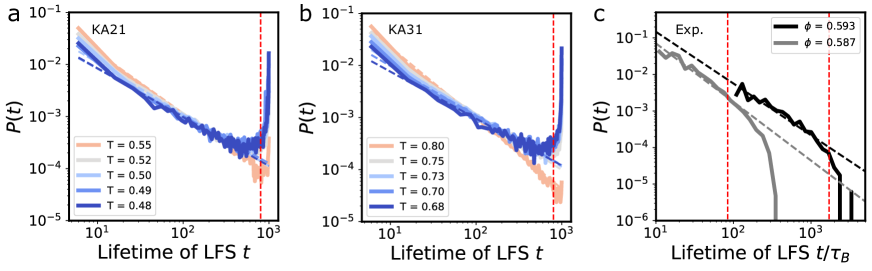
Figure S2: The probability distribution of LFS lifetime. (a) KA2:1. (b) KA3:1. (c) Colloidal experiments.

After identifying the LFS, we select those which survive over 80% of the duration of the sub-trajectory (i.e. longer than 800 LJ time units). We choose the 80% criterion on the basis of the probability distribution of LFS lifetime, which serves as a turnover point [Fig. S2]. We consider those clusters to be long-lived LFS. It should be noted that here we do not require these clusters to be in LFS for 800 LJ time units continuously.

In the following, we consider exclusively long-lived LFS following the discussion above.

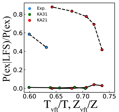
Figure 2: Anti-correlation between LFS and excitations. Thermalised/instantaneous data from Ortlieb et al. (2023) (red dashed line). Solid lines correspond to the anti-correlation between long-lived LFS and excitations in the inherent states.

II.5 Calculation of the separation between LFS and excitations

If an LFS particle fits the criterion of “long-lived”, we label it as “LFS” throughout the whole trajectory. For excitations, we label the particle as “EX” during $[t_{0}-t_{a},t_{0}+t_{a}]$, where $t_{0}$ is when the excitation happens. Then we calculate the conditional probability $P(EX|LFS)$ of each frame, and the probability of finding excitations $P(EX)$ of each frame. Thus, we can use $P(EX|LFS)\ P(EX)$ to indicate the probability of excitations overlapping with LFS. For each temperature, we take the average $P(EX|LFS)/P(EX)$ of all frames in 10 trajectories.

With this labelling method, we compute the distance between excitations and their closest LFS “center”. We choose the particle closest to the geometric center of the cluster as the “center” particle. As shown in Fig. 1(b), the central particle of the antiprism is the geometric centre (indicated with a black dot). In the case of the defective icosahedron we consider the particle closest to the centre of mass of the LFS. This particle (indicated in Fig. 1(b)] is 0.45$\sigma$ away from the center of mass. We also consider clusters survive over 40% time of the whole trajectory to be long-lived LFS (longer than $10^{2}$ Brownian time $\tau_{B}$), according to the LFS lifetime distribution Fig. S2.

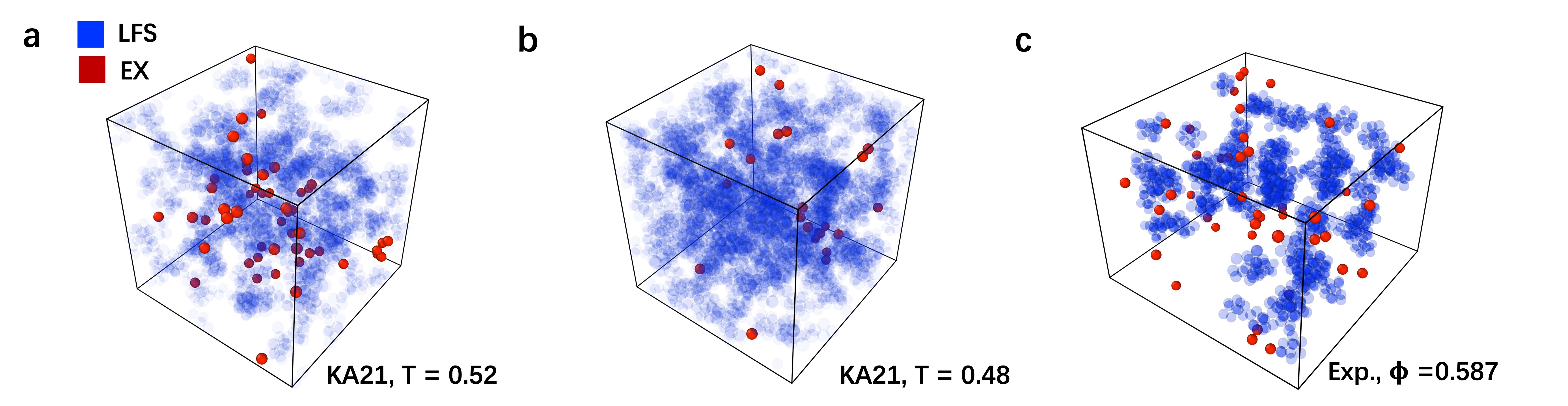
Figure 3: Representative snapshots of high temperature (a) and low temperature (b) in KA2:1. Particles in LFS are rendered in blue and excitations are rendered in red. (c) A representative snapshot of the experimental colloidal system.

Then we compute the average distance of all excitations in all frames in all trajectories. We choose these different time criteria between the LFS and excitations because in the case of an excitation occurring inside in LFS, its movement would naturally distort the LFS and likely lead to the LFS no longer being detected. If the LFS is no longer detected, then its separation from the excitation would not be counted, which would have severe consequences for our analysis. We have found that the method we implemented avoids this problem.

III Results

We begin our results section by discussing the glassforming behavior of the systems considered. We probe the increase in relaxation via an Angell plot, and evaluate the increase in LFS upon supercooling. We also determine the drop in population of excitations with supercooling. We then move on to consider the spatial relationship of LFS and excitations, starting with some snapshots, before presenting our protocol to determine the separation between excitations and LFS. We then investigate local packing of particles in excitations and LFS.

III.1 The proportion of LFS and excitations at deep supercooling

Fig. 1(a) shows a so-called Angell plot of relaxation time $\tau_{\alpha}$ with respect to inverse temperature $1/T$ for the Kob-Andersen binary (KA) mixture and reduced pressure $Z$ for the experimental hard-sphere colloidal system. Here we fit $\tau_{\alpha}$ with the Vogel–Fulcher–Tamman (VFT) equation,

$${\tau}_{\alpha}^{\mathrm{\\ sim}}={\tau}_{0}\exp\left(\frac{D{T}_{{{{{{{{\rm{vft}}}}}}}}}}{T-{T}_{{{{{{{{\rm{vft}}}}}}}}}}\right)\quad,{\tau}_{\alpha}^{\exp}={\tau}_{0}\exp\left(\frac{D{Z}}{{Z}_{{{{{{{{\rm{vft}}}}}}}}}-Z}\right)$$ (3)

for simulations and experiments, respectively. Here $D$ is a system-dependent constant. We focus on the region at deeper supercooling than the mode-coupling cross-over as indicated by the blue shading. The mode-coupling crossover was taken from Ortlieb et al. (2023) to be $T_{\mathrm{mct}}=0.55\pm 0.09$ and $0.7\pm 0.1$ for the KA 2:1 and 3:1 systems respectively. For the experiments, we took a volume fraction $\phi_{\mathrm{mct}}=0.58$ van Megen et al. (1998) which corresponds to a reduced pressure $Z_{\mathrm{mct}}=23.23$.

In Fig. 1 we see that with the decrease in temperature, in the case of the simulations, and increase in reduced pressure for the experiments, the proportion of LFS grows [Fig. 1(b)], while the proportion of excitations decreases, consistent with previous results Ortlieb et al. (2023), Fig. 1(c).

III.2 The anti-correlation between LFS and excitations

We further calculate the probability of overlap between LFS and excitations, and it turns out that the probability is generally very small (Fig. 2). Representative snapshots also confirm that LFS and excitations are generally not overlapped (Fig. 3a-c) (indicating that there may be a spatial separation in between.)

An anti-correlation between LFS and excitations was found by Ortlieb et al. (2023). That work considered thermalized configurations. Here we show that the anti-correlation is robust to inherent states and we also consider experimental data. In fact, while the thermalized configurations with instantaneous LFS show a weaker anti-correlation at higher temperatures, the long-lived LFS considered here used here have a strong anti-correlation at all temperatures as we see in Fig. 2. We return to this point below.

III.3 The spatial separation between LFS and excitations

To further probe the anti-correlation between LFS and excitations and their spatial separation, we calculate the distance between LFS and excitations. We compute the distance of an excitation particle to its closest LFS center (denoted by $d$). Figures 4(a) and 5(a) represent some typical scenarios where the excitation particle is inside the LFS or outside the LFS.

We first choose particles in excitations and compute the distance $d$, and the probability distribution $P(d)$ is shown in Fig.  4(b). However, since the population of LFS increases with supercooling [Fig. 1(b)], then one expects that the separation of a particle chosen at random and the nearest LFS particle to it should decrease with supercooling, quite the opposite trend of increasing separation between LFS and excitations that our hypothesis would suggest. This effect seems to lead to a decrease in typical separation between LFS and excitation particles.

To compensate for this effect of the decrease in excitation–LFS separation, which we expect to be driven by the increase in LFS particles with supercooling, we proceed as follows. We pick some random particles and also compute this probability distribution $P_{\mathrm{rand}}(d)$ which we show in Fig. 4(c). By normalizing the LFS-excitation separation distribution by that of the random particles – LFS, we can compensate for the effect of the increasing LFS population at deep supercooling. Thus by calculating $P(d)/P_{\mathrm{rand}}(d)$, we obtain Fig. 4(d), which reveals the distribution of distances between LFS centers and excitations compared with a random particle.

The black dotted line in Fig. 4(d) indicates that the probability of finding excitation particles here is the same as random particles. Thus, compared to random particles, fewer excitations happen inside LFS (position 1), and more excitations outside LFS (positions 2 and 3). The dashed line in Fig. 4(d) is the linear fit $P(d)/P_{\mathrm{rand}}(d)$, indicating that there is a trend that excitations are more likely to occur outside LFS. (This trend may be more obvious at low temperatures). This spatial separation is also observed in the KA3:1 mixture [Fig. 4(e)] and experimental colloidal system (Fig. 5). Thus, for the systems considered, there is a tendency towards excitations occurring outside the LFS upon supercooling.

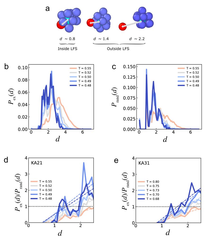
Figure 4: The spatial relationship between excitations and LFS for the computer simulations. (a) Some typical scenarios of particles inside LFS and outside LFS. $d$ is the distance from one particle and its closest LFS center. (b) The probability distribution of the distance $d$ from one excitation to its closest LFS center. (c) The probability distribution of the distance $d$ from one random particle to its closest LFS center. (d) Scaled excitation–LFS center distance. [(b) normalized by (c)]. That is to say, the effects of the increasing LFS population with supercooling have been removed. Dashed lines in (d) are linear fits. Data above the black dotted line, indicates that excitations are more likely to be found at this distance from the LFS center compared to random particles. (e) The scaled excitation–LFS distance for the KA 3:1 system. That is to say, the sane representation as (d).

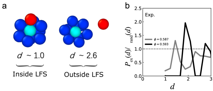
Figure 5: The spatial relationship between excitations and LFS for the experiments. (a) Some typical scenarios of particles inside LFS and outside LFS. $d$ is the distance from one particle and its closest LFS center. (b) Scaled excitation–LFS center distance. This corresponds to Figs. 4(d,e).

III.4 Voronoi Cell Volumes

To investigate why excitations are more likely to occur outside the LFS) we compute the volume of the Voronoi cell for each particle. We consider A and B particles for the KA2:1 composition n Fig. 6, where we plot the distribution of Voronoi volumes for particles in LFS and also those in excitations. While the distributions overlap, there is a clear trend of LFS particles having a small Voronoi volume, ie being well packed. The opposite trend is seen for excitations whose larger Voronoi volumes indicate poorer packing. In the case of the smaller B particles, the trend is stronger. We show the case for the KA 3:1 composition in the SM. For the experimental data, errors in coordinate tracking hamper this analysis, moreover for a given coordinate, we do not know the diameter of a given particle in this polydisperse system Ivlev, A. and Lowen, H and Morfill, G. E. and Royall, C. P. (2012); Royall et al. (2023).

Figure 6: Volumes of Voronoi cells for particles in LFS and excitations in the KA 2:1 composition. (a) The probability distribution of A particles. (b) The probability distribution of B particles. The vertical black line is the average of all particles. Solids lines are particles in excitations, dashes are particles in LFS.

IV Discussion

We have investigated the spatial relationship between LFS and excitations in simulations and experiments on model glassformers. This work was motivated by the recent observation of a signficant anti-correlation between excitations and LFS Ortlieb et al. (2023). This seems to be stronger than is the case for earlier work which examined the relation between local structure and dynamic heterogeneity at weaker supercooling Charbonneau et al. (2012); Malins et al. (2013a).

Here we found a significant anti-correlation between long-lived LFS and excitations. This is stronger than that observed previously, Ortlieb et al. (2023) due to our use of long-lived LFS and using inherent state coordinates. Some comments are in order here. In a series of papers Speck and co-workers explored the dynamical phase transition of dynamic facilitation theory in a number of model glassformers in both simulations and experiment Speck et al. (2012); Pinchaipat et al. (2017); Turci et al. (2017, 2018); Royall et al. (2020); Campo and Speck (2019). This transition – obtained using short (a few $\tau_{\alpha}$) and small (typically around 100-200 particles) trajectories – exists between a so-called active phase (similar to the normal supercooled liquid) and an inactive phase, whose dynamics are too slow to be measured on the simulation timescale. This transition is driven by the time–averaged population of LFS. Therefore, the anti-correlation between excitations (a feature of the active phase) and long-lived LFS (which are likley related to the time-averaged LFS of the inactive phase) may be taken as consistent with the dynamical phase transition. We therefore expect that long-lived LFS are some measure of local stability in the supercooled liquid.

The deeper supercooling now possible in both experiment and computer simulation enables us to identify excitations (which are hard to detect for $T>T_{\mathrm{mct}}$ and $Z<Z_{\mathrm{mct}}$). Earlier work often struggled to find a significant coupling between local structure and dynamic heterogeneity Charbonneau et al. (2012); Malins et al. (2013a).

It has been found that there is a rather weaker anti-correlation between LFS and Co-operatively Re-arranging Regions (CRRs) which are the elementary units of relaxation in RFOT and Adam-Gibbs thermodynamic-based theories Ortlieb et al. (2023). If we imagine that the long-lived LFS are representative of the emerging solid glass, the enhanced anti-correlation of the excitations with respect to the CRRs raises questions about these relaxation mechanisms. It has been suggested that CRRs may be comprised of many excitations Ortlieb et al. (2023). The lifetimes even of the long-lived LFS are very much smaller than the structural relaxation time $\tau_{\alpha}$ and indeed the timescale associated with CRRs, which reaches $1.1\times 10^{5}$ LJ time units for the lowest temperature studied Ortlieb et al. (2023). Such a timescale of course presents great challenges for the frequency of sampling that we use here. Here, we have focussed on the excitations, but the link between excitations and the much longer timescale CRRs, and the LFS remains an intriguing and challenging topic for a future investigation.

V Conclusion

In this work, we have analysed particle-resolved data from both GPU simulations and experiments in deeply supercooled liquids, with a focus on detecting excitations and identifying long-lived locally favoured structures. We have shown that with the decrease in temperature or increase in reduced pressure, the proportion of LFS grows while the proportion of excitations decreases. Moreover, a strong and robust anti-correlation between long-lived LFS and excitations has been identified. By considering inherent states in our computer simulations we have obtained a stronger anti-correlation than that previously found Ortlieb et al. (2023). To further probe this anti-correlation, we have computed the distance between excitations and long-lived LFS and excitations. Notably, excitations are more likely to occur outside long-lived LFS, demonstrating there is a spatial separation between the two. This spatial separation may be attributed to the well-packed nature of long-lived LFS, as revealed by the analysis of the volumes of the Voronoi cells for each particle.

Our work provides a picture of structural relaxation via excitations occurring in regions of the system outside long-lived LFS. We hope this will stimulate further investigations of the relationship between structure and dynamics in the deeply supercooled regime of glassforming systems which is now accessible.

Data Availability Statement

Data and code are available upon reasonable request.

VI Supporting Information

	KA2:1	KA3:1	Experiment
$T_{VFT}$ or $Z_{VFT}$	$0.35$	$0.48$	$41$
$\tau_{0}$	$0.09$	$0.07$	$0.63$
$D$	$2.68$	$2.99$	$2.21$

Table S1: VFT parameters fitted to the various systems considered.

	KA2:1	KA3:1	Experiment
$T_{on}$ or $Z_{on}$	$0.75$	$1.2$	$23$
$E_{a}$	$5.96$	$8.30$	$1.19$

Table S2: Scaling of the population of particles in excitations.

Figure S1: The spatial separation in KA3:1 system. (a) The probability distribution of the distance $d$ between excitations and their closest LFS centers. (b) The probability distribution of the distance $d$ between random particles and their closest LFS centers. The ratio of the data plotted in (a) and (b) is shown in Fig. 4(e) in the main text.

References

- Berthier and Biroli (2011) L. Berthier and G. Biroli, Rev. Mod. Phys. 83, 587 (2011), ISSN 0034-6861, 1539-0756.
- Adam and Gibbs (1965) G. Adam and J. Gibbs, J. Chem. Phys. 43, 139 (1965).
- Lubchenko and Wolynes (2007) V. Lubchenko and P. G. Wolynes, Annu. Rev. Phys. Chem. 58, 235 (2007).
- Chandler and Garrahan (2010) D. Chandler and J. P. Garrahan, Annu. Rev. Phys. Chem. 61, 191 (2010), ISSN 0066-426X, 1545-1593.
- Speck (2019) T. Speck, J. Stat. Mech. 2019, 084015 (2019), ISSN 1742-5468, eprint 1902.07768.
- Tarjus et al. (2005) G. Tarjus, S. A. Kivelson, Z. Nussinov, and P. Viot, J. Phys.: Condens. Matter 17, R1143 (2005), ISSN 0953-8984, 1361-648X.
- Royall and Williams (2015) C. P. Royall and S. R. Williams, Physics Reports 560, 1 (2015), ISSN 03701573.
- Leocmach and Tanaka (2012) M. Leocmach and H. Tanaka, Nat Commun 3, 974 (2012), ISSN 2041-1723.
- Hunter and Weeks (2012) G. L. Hunter and E. R. Weeks, Rep Prog Phys p. 31 (2012).
- Ivlev, A. and Lowen, H and Morfill, G. E. and Royall, C. P. (2012) Ivlev, A. and Lowen, H and Morfill, G. E. and Royall, C. P., Complex Plasmas and Colloidal Dispersions: Particle-Resolved Studies of Classical Liquids and Solids (World Scientific Publishing Co., Singapore Scientific, Singapore, 2012).
- Royall et al. (2023) C. P. Royall, P. Charbonneau, M. Dijkstra, J. Russo, F. Smallenburg, T. Speck, and C. Valeriani, acceoted in Rev. Mod. Phys. online at ArXiV p. 2305.02452 (2023).
- Gokhale et al. (2016) S. Gokhale, A. K. Sood, and R. Ganapathy, Adv. Phys. 65, 363 (2016).
- Charbonneau and Reichman (2005) P. Charbonneau and D. Reichman, J. Stat. Mech.: Theory and Experiment p. P05013 (2005).
- Ninarello et al. (2017) A. Ninarello, L. Berthier, and D. Coslovich, Phys. Rev. X 7, 021039 (2017), ISSN 2160-3308.
- Scalliet et al. (2022) C. Scalliet, B. Guiselin, and L. Berthier, ArXiV p. 2207.00491 (2022).
- Bailey et al. (2015) N. P. Bailey, T. S. Ingebrigtsen, J. S. Hansen, A. A. Veldhorst, L. Bøhling, C. A. Lemarchand, A. E. Olsen, A. K. Bacher, H. Larsen, J. C. Dyre, et al., arXiv p. 1506.05094 (2015).
- Ortlieb et al. (2023) L. Ortlieb, T. S. Ingebrigtsen, J. E. Hallett, F. Turci, and C. P. Royall, Nature Communications 14, 2621 (2023).
- Brambilla et al. (2009) G. Brambilla, D. El Masri, M. Pierno, L. Berthier, L. Cipelletti, G. Petekidis, and A. B. Schofield, Phys. Rev. Lett. 102, 085703 (2009).
- Hallett et al. (2018) J. E. Hallett, F. Turci, and C. P. Royall, Nat Commun 9, 3272 (2018), ISSN 2041-1723.
- Hasyim and Mandadapu (2024) M. R. Hasyim and K. K. Mandadapu, Proc. Nat. Acad. Sci. 121, e2322592121 (2024).
- Keys et al. (2011) A. S. Keys, L. O. Hedges, J. P. Garrahan, S. C. Glotzer, and D. Chandler, Phys. Rev. X 1, 021013 (2011), ISSN 2160-3308.
- Hasyim and Mandadapu (2021) M. R. Hasyim and K. K. Mandadapu, ArXiV p. 2103.03015 (2021).
- Gokhale et al. (2014) S. Gokhale, K. H. Nagamanasa, R. Ganapathy, and A. K. Sood, Nature Comm. 5, 4685 (2014).
- Nagamanasa et al. (2015) S. Nagamanasa, K. H.Nagamanasa, A. K. Sood, and R. Ganapathy, Nature Phys 11, 403 (2015).
- Turci et al. (2017) F. Turci, C. P. Royall, and T. Speck, Phys. Rev. X 7, 031028 (2017).
- Berthier et al. (2017) L. Berthier, P. Charbonneau, D. Coslovich, A. Ninarello, M. Ozawa, and S. Yaida, Proc Natl Acad Sci USA 114, 11356 (2017), ISSN 0027-8424, 1091-6490.
- Berthier et al. (2019) L. Berthier, M. Ozawa, and C. Scalliet, J. Chem. Phys. 150, 160902 (2019), ISSN 0021-9606, 1089-7690.
- Royall et al. (2020) C. P. Royall, F. Turci, and T. Speck, J Chem Phys 153, 090901 (2020), ISSN 0021-9606, 1089-7690.
- Speck et al. (2012) T. Speck, A. Malins, and C. P. Royall, Phys. Rev. Lett. 109, 195703 (2012).
- Malins et al. (2013a) A. Malins, J. Eggers, H. Tanaka, and C. P. Royall, Faraday Discussions 167, 405 (2013a).
- Kawasaki et al. (2007) T. Kawasaki, T. Araki, and H. Tanaka, Phys. Rev. Lett. 99, 215701 (2007).
- Tamborini et al. (2015) E. Tamborini, C. P. Royall, and P. Cicuta, J. Phys.: Condens. Matter 27, 194124 (2015).
- Charbonneau et al. (2012) B. Charbonneau, P. Charbonneau, and G. Tarjus, Phys. Rev. Lett. 108, 035701 (2012).
- Richard et al. (2020) D. Richard, M. Ozawa, S. Patinet, E. Stanifer, B. Shang, S. A. Ridout, B. Xu, G. Zhang, P. K. Morse, J.-L. Barrat, et al., Phys. Rev. Materials 4, 113609 (2020).
- Tong and Tanaka (2018) H. Tong and H. Tanaka, 8, 011041 (2018).
- Cubuk et al. (2015) E. D. Cubuk, S. S. Schoenholz, J. M. Rieser, B. D. Malone, J. Rottler, D. J. Durian, E. Kaxiras, and A. J. Liu, Phys. Rev. Lett. 114, 108001 (2015).
- Malins et al. (2013b) A. Malins, S. R. Williams, J. Eggers, and C. P. Royall, The Journal of Chemical Physics 139, 234506 (2013b), ISSN 0021-9606, 1089-7690.
- Hocky et al. (2014) G. M. Hocky, D. Coslovich, A. Ikeda, and D. Reichman, Phys. Rev. Lett. 113, 157801 (2014).
- Royall et al. (2018) C. P. Royall, S. R. Williams, and H. Tanaka, The Journal of chemical physics 148 (2018).
- Bailey et al. (2017) N. Bailey, T. Ingebrigtsen, J. S. Hansen, A. Veldhorst, L. Bøhling, C. Lemarchand, A. Olsen, A. Bacher, L. Costigliola, U. Pedersen, et al., SciPost Physics 3, 038 (2017).
- Plimpton (1995) S. Plimpton, J. Comp. Phys. 117, 1 (1995), ISSN 0021-9991, URL http://www.sciencedirect.com/science/article/pii/S002199918571039X.
- Thompson et al. (2022) A. P. Thompson, H. M. Aktulga, R. Berger, D. S. Bolintineanu, W. M. Brown, P. S. Crozier, P. J. in’t Veld, A. Kohlmeyer, S. G. Moore, T. D. Nguyen, et al., Computer Physics Communications 271, 108171 (2022).
- Royall et al. (2015) C. P. Royall, A. Malins, A. J. Dunleavy, and R. Pinney, Journal of Non-Crystalline Solids 407, 34 (2015), ISSN 00223093.
- Berthier and Witten (2009) L. Berthier and T. A. Witten, Phys. Rev. E 80, 021502 (2009), ISSN 1539-3755, 1550-2376.
- Coslovich and Pastore (2007) D. Coslovich and G. Pastore, The Journal of Chemical Physics 127, 124504 (2007), ISSN 0021-9606, 1089-7690.
- Crowther et al. (2015) P. Crowther, F. Turci, and R. C. P., J. Chem. Phys. 143, 044503 (2015).
- Dunleavy et al. (2015) A. J. Dunleavy, K. Wiesner, R. Yamamoto, and C. P. Royall, Nature Communications 6, 6089 (2015).
- van Megen et al. (1998) W. van Megen, T. C. Mortensen, and S. R. Williams, Phys. Rev. E. 58, 6073 (1998).
- Pinchaipat et al. (2017) R. Pinchaipat, M. Campo, F. Turci, J. Hallett, T. Speck, and C. P. Royall, Phys. Rev. Lett. 119, 028004 (2017).
- Turci et al. (2018) F. Turci, T. Speck, and C. P. Royall, ArXiV 1804.00929 (2018).
- Campo and Speck (2019) M. Campo and T. Speck, ArXiV p. 1910.12045 (2019).