Improved identification of breakpoints in piecewise regression and its applications

Abstract

Identifying breakpoints in piecewise regression is critical in enhancing the reliability and interpretability of data fitting. In this paper, we propose novel algorithms based on the greedy algorithm to accurately and efficiently identify breakpoints in piecewise polynomial regression. The algorithm updates the breakpoints to minimize the error by exploring the neighborhood of each breakpoint. It has a fast convergence rate and stability to find optimal breakpoints. Moreover, it can determine the optimal number of breakpoints. The computational results for real and synthetic data show that its accuracy is better than any existing methods. The real-world datasets demonstrate that breakpoints through the proposed algorithm provide valuable data information.

1 Introduction

Piecewise regression, also known as segmented regression, is a powerful statistical technique used to model and analyze variables whose relationship can vary over different intervals of an independent variable [1, 22]. Unlike traditional regression models, which assume a uniform effect across the entire range of data, piecewise regression allows for varying slopes and intercepts within predefined segments of the data set. This method is particularly useful in fields such as economics, epidemiology, and environmental science, where abrupt changes are often expected as a result of interventions or natural thresholds [18].

Piecewise regression allows for more accurate modeling and prediction by dividing the data into segments and fitting a polynomial regression model to each segment. There are various fields such as economics and finance [29], engineering [15, 34], energy and power systems [9, 14, 16], network flow [23], biological and healthcare [13, 32, 33] using piecewise regression.

Continuity at breakpoints in piecewise regression is a critical factor in enhancing the reliability and interpretability of the model. In situations with multiple change points, continuous models can stably reflect changes in the data, thereby improving the stability of the model and predictive performance [10]. Furthermore, maintaining continuity in regression models with unknown breakpoints provides more realistic and interpretable results [22]. Ensuring continuity in linear models with multiple structural changes more accurately captures the structural changes in the data [2].

The key challenge in piecewise regression is to accurately identify the points where the relationship of variables changes, known as breakpoints or change points. The model’s accuracy heavily depends on correctly identifying these points, as they define the boundaries between intervals where different relationships apply. The detection of breakpoints has been addressed using various statistical and computational methods. Traditional approaches often involve manually setting potential breakpoints based on domain knowledge or using grid search techniques to systematically evaluate a range of breakpoints [3]. More advanced techniques include algorithms such as binary segmentation and dynamic programming, which are designed to optimize the fit of piecewise models by iteratively testing potential breakpoints and evaluating their impact on the accuracy of the model [6, 12, 18, 30]. Despite their effectiveness, these methods can be computationally intensive and may not scale well with large datasets or complex models. Various methods have been proposed, including methods based on integer linear programming [35], the $\ell_{1}$ trend filter [19], which is a variant of the Hodrick-Prescott (H-P) filter, recently proposed adaptive piecewise regression using optimization techniques [17, 28], and a column generation-based heuristic method [31].

In this study, we present an improved algorithm for identifying breakpoints in piecewise regression using the greedy algorithm approach. A greedy algorithm is an intuitive and simple method for solving optimization problems, characterized by making locally optimal choices at each step and then finding the global optimum. Since it incrementally constructs the solution and selects the most immediately beneficial choice at each step, it is often preferred because it is simple and easy to implement compared to more complex methods such as dynamic programming. However, it is important to note that greedy algorithms do not always guarantee a globally optimal solution and can sometimes converge to a local minimum.

In addition, determining the optimal number and location of breakpoints in a piecewise regression is important to improve the accuracy and interpretability of the model. Too many breakpoints can lead to overfitting, and not enough breakpoints can lead to underfitting of the data. The optimal number and location of breakpoints ensure that each segment of the regression model effectively represents the underlying data, providing more reliable predictions and insights.

Our main contributions in this paper are summarized in brief as follows.

• The proposed algorithm accurately identifies breakpoints to minimize error. The piecewise regression with the proposed algorithm has a lower loss than other existing methods.

• The proposed algorithm can determine the optimal number of breakpoints. It can be used to estimate the proper number of breakpoints for the data.

• The algorithm has a fast convergence rate and stability to find optimal breakpoints. Moreover, it significantly reduces computational cost.

This paper is structured as follows. Section 2 introduces continuous piecewise polynomial regression from the optimization point of view. The proposed method and its algorithms are presented in Section 3. Section 4 presents the results of numerical experiments that use both synthetic and real data to demonstrate the performance of the proposed method and efficient breakpoint identification. The last section concludes the paper with a summary of our findings, discusses potential applications of this research, and suggests directions for future work in this area.

Notations:

Let $\mathbb{R}$ (resp. $\mathbb{N}$) be the set of real(resp. natural) numbers. For a vector $\bm{x}$, $\|\bm{x}\|_{2}$ denotes the Euclidean norm. The superscript $T$ denotes the transpose operator. The mean square error (MSE) is defined as the difference between the regressor and the observed data:

$$\operatorname{MSE}\left(\bm{\hat{y}},\bm{y}\right):=\frac{1}{n}\left\|\hat{\bm{y}}-\bm{y}\right\|_{2},$$

where $\bm{y}$ and $\hat{\bm{y}}$ in $\mathbb{R}^{n}$ are the observed data and the regressors, respectively.

2 Continuous piecewise polynomial regression

For given data $\{(x_{i},y_{i})\}_{i=1}^{n}\subset\mathbb{R}^{2}$, consider a continuous function $f$ depicting a slowly varying trend

$$y_{i}=f(x_{i})+\varepsilon_{i},$$

under rapidly varying random noise $\varepsilon_{i}\in\mathbb{R}$. Here, $x_{i}$ represents observation time in ascending order, i.e., $x_{1}\leq x_{2}\leq\cdots\leq x_{n}$, sampled from a time interval randomly or uniformly. To describe $f$ properly, a popular family of functions such as polynomials and exponential functions can be used [17]. To allow abrupt changes in shape and to preserve simplicity, piecewise polynomials are adopted.

First, assume that the breakpoints $\xi_{1},\ldots,\xi_{k-1}$, with $\xi_{1}<\cdots<\xi_{k-1}$ are given for a fixed $k\geq 2$ and that each breakpoint $\xi_{j}$ does not overlap with the data $x_{i}$. For convenience of notation, set $\xi_{0}=x_{1}$ and $\xi_{k}=x_{n}$. And define subinterval $I_{j}:=[\xi_{j-1},\xi_{j}]$ for $j=1,\ldots,k$. By assumption, each data $x_{i}$ is contained in one single subinterval. The goal is to construct a continuous polynomial regression of degree $d$. Mathematically, the piecewise polynomial regression can be formulated as a typical least squares problem with linear equality constraints as follows:

$$\operatorname*{minimize}_{\theta_{ij}}\sum\limits_{j=1}^{k}\sum\limits_{x_{i}\in I_{j}}\left(p_{j}(x_{i})-y_{i}\right)^{2}$$ (2.1)

$$\text{subject to }p_{j}(\xi_{j})=p_{j+1}(\xi_{j}),\quad j=1,\ldots,k-1,$$

where $p_{j}:I_{j}\rightarrow\mathbb{R}$ is a $d$th degree polynomial for all $j=1,\ldots,k$, given by $p_{j}(x)=\theta_{0j}+\theta_{1j}x+\theta_{2j}x^{2}+\cdots+\theta_{dj}x^{d}$.

For $z\in\mathbb{R}$ denote

$$\bm{v}(z):=\begin{bmatrix}1&z&z^{2}&\cdots&z^{d}\end{bmatrix}^{T}.$$

Define a Vandermonde matrix [24] of the interval $I_{j}$ as

$$\bm{V}(I_{j}):=\begin{bmatrix}\rule[2.15277pt]{10.76385pt}{0.5pt}\,\bm{v}(z_{1,j})^{T}\,\rule[2.15277pt]{10.76385pt}{0.5pt}\\ \rule[2.15277pt]{10.76385pt}{0.5pt}\,\bm{v}(z_{2,j})^{T}\,\rule[2.15277pt]{10.76385pt}{0.5pt}\\ \vdots\\ \vdots\\ \rule[2.15277pt]{10.76385pt}{0.5pt}\,\bm{v}(z_{m_{j},j})^{T}\,\rule[2.15277pt]{10.76385pt}{0.5pt}\end{bmatrix},$$ (2.2)

where $z_{1,j}\leq z_{2,j}\leq\cdots\leq z_{m_{j},j}$ are all elements $x_{i}$ in $I_{j}$.

The optimization problem (2.1) can be rewritten as follows:

$$\operatorname*{minimize}_{\bm{\theta}}\left\|\bm{X}\bm{\theta}-\bm{y}\right\|^{2}_{2}$$ (2.3)

$$\text{subject to }\bm{C}_{\bm{\xi}}\bm{\theta}={\bm{0}},$$

where

$$\bm{X} =\begin{bmatrix}\bm{V}(I_{1})&\bm{0}&\cdots&\bm{0}\\ \bm{0}&\bm{V}(I_{2})&\cdots&\bm{0}\\ \vdots&\vdots&\ddots&\vdots\\ \bm{0}&\bm{0}&\cdots&\bm{V}(I_{k})\\ \end{bmatrix},$$

$$\bm{\theta} =\begin{bmatrix}\theta_{01}&\theta_{11}&\cdots&\theta_{d1}&\theta_{02}&\theta_{12}&\cdots&\theta_{dk}\end{bmatrix}^{T},$$

$$\bm{y} =\begin{bmatrix}y_{1}&y_{2}&\cdots&y_{n}\end{bmatrix}^{T},$$

$$\bm{C}_{\bm{\xi}} =\begin{bmatrix}\bm{v}(\xi_{1})^{T}&-\bm{v}(\xi_{1})^{T}&&&\bm{0}\\ &\bm{v}(\xi_{2})^{T}&-\bm{v}(\xi_{2})^{T}&&\\ &&\ddots&\ddots&\\ \bm{0}&&&\bm{v}(\xi_{k-1})^{T}&-\bm{v}(\xi_{k-1})^{T}\\ \end{bmatrix},$$

$$\bm{\xi} =\begin{bmatrix}\xi_{1}&\xi_{2}&\cdots&\xi_{k-1}\end{bmatrix}^{T}.$$

The Lagrangian for optimization problem (2.3) can be expressed as follows:

$$\mathcal{L}(\bm{\theta},\bm{\lambda})=\bm{\theta}^{T}\bm{X}^{T}\bm{X}\bm{\theta}-2\bm{y}^{T}\bm{X}\bm{\theta}+\bm{y}^{T}\bm{y}+\bm{\lambda}^{T}\bm{C}_{\bm{\xi}}\bm{\theta}.$$

Since the optimization problem (2.3) is convex to find its global minimum, it is enough to find a point where the gradient $\nabla\mathcal{L}$ vanishes. Setting $\nabla\mathcal{L}=0$ results in the equations

$$\begin{cases}\cfrac{\partial\mathcal{L}}{\partial\bm{\theta}}=2\bm{X}^{T}\bm{X}\bm{\theta}-2\bm{X}^{T}\bm{y}+\bm{C}_{\bm{\xi}}^{T}\bm{\lambda}=\bm{0},\\ \cfrac{\partial\mathcal{L}}{\partial\bm{\lambda}}=\bm{C}_{\bm{\xi}}\bm{\theta}=\bm{0}.\end{cases}$$

Then it can be rewritten in matrix form as follows.

$$\begin{bmatrix}2\bm{X}^{T}\bm{X}&\bm{C}_{\bm{\xi}}^{T}\\ \bm{C}_{\bm{\xi}}&\bm{0}\end{bmatrix}\begin{bmatrix}\bm{\theta}\\ \bm{\lambda}\end{bmatrix}=\begin{bmatrix}2\bm{X}^{T}\bm{y}\\ \bm{0}\end{bmatrix}.$$ (2.4)

The block matrix in equation (2.4) is called the KKT matrix and is nonsingular, so the optimal solution can be found [4, 7, 8]. Then one can solve the linear system to find the solution (see Algorithm 1).

Function Piecewise_regression 

       Input : $\{(x_{i},y_{i})\}_{i=1}^{n}\subset\mathbb{R}^{2}$: data; $\bm{\xi}\in\mathbb{R}^{k+1}$: breakpoints; $d\in\mathbb{N}$: degree

       Output : $\hat{y}_{1},\ldots,\hat{y}_{n}$: regressors of observed values $y_{1},\ldots,y_{n}$

       Construct $\bm{X}$ from $x_{1},\ldots,x_{n}$

       Construct $\bm{C}_{\bm{\xi}}$ from $\xi_{1},\ldots,\xi_{k-1}$

       $\bm{A}$ $\leftarrow$ $\begin{bmatrix}2\bm{X}^{T}\bm{X}&\bm{C}_{\bm{\xi}}^{T}\\ \bm{C}_{\bm{\xi}}&\bm{0}\end{bmatrix}$

       $\bm{b}$ $\leftarrow$ $\begin{bmatrix}2\bm{y}^{T}\bm{X}&\bm{0}\end{bmatrix}^{T}$

       $\bm{\theta}$ $\leftarrow$ solve (2.4)

      $\hat{\bm{y}}$ $\leftarrow$ $\bm{X}\bm{\theta}$

      

end

Algorithm 1 Piecewise polynomial regression

3 Methodology

If the breakpoints $\bm{\xi}=[\xi_{1}~{}\xi_{2}~{}\cdots~{}\xi_{k-1}]^{T}$ are fixed, then the piecewise polynomial regression can be obtained using Algorithm 1. However, the location of breakpoints for real data is in general unknown. Even, the number of breakpoints is unknown. Both the number and location of breakpoints must be chosen appropriately to get a regression that fits the data. First, assume that the number of breakpoints is given. To find the optimal location of breakpoints $\bm{\xi}$ and the optimal coefficients of polynomials $\bm{\theta}=[\theta_{01},~{}\theta_{11},~{}\cdots,~{}\theta_{d1},~{}\theta_{02},~{}\theta_{12},~{}\cdots,~{}\theta_{dk}]^{T}$, one can solve the optimization problem.

$$\operatorname*{minimize}_{\bm{\theta},~{}\bm{\xi}}\sum\limits_{j=1}^{k}\sum\limits_{x_{i}\in I_{j}}\left(p_{j}(x_{i})-y_{i}\right)^{2}$$ (3.1)

$$\text{subject to }p_{j}(\xi_{j})=p_{j+1}(\xi_{j}),\quad j=1,\ldots,k-1.$$

where $p_{j}:I_{j}\rightarrow\mathbb{R}$ is a $d$th degree polynomial for all $j=1,\ldots,k$, given by $p_{j}(x)=\theta_{0j}+\theta_{1j}x+\theta_{2j}x^{2}+\cdots+\theta_{dj}x^{d}$.

Since this optimization problem is nonconvex [17], it is not easy to solve the problem. Due to the number of too many breakpoint candidates, numerical algorithms may need an extensive computational cost. To overcome this situation, our proposed method selects each breakpoint from a certain finite set. It is important to choose a suitable set for given data. In this paper, consider the following set for the candidates of breakpoints:

$$\mathcal{X}=\left\{\dfrac{x_{i}+x_{i+1}}{2}\Big{|}i=1,2,\ldots,n-1\right\}.$$

For convenience in explaining the proposed method for updating the breakpoints, assume that $x_{1}<x_{2}<\cdots<x_{n}$. Therefore, the optimization problem (3.1) is relaxed to the following.

$$\operatorname*{minimize}_{\bm{\theta},~{}~{}\bm{\xi}\subseteq\mathcal{X}}\sum\limits_{j=1}^{k}\sum\limits_{x_{i}\in I_{j}}\left(p_{j}(x_{i})-y_{i}\right)^{2}$$ (3.2)

$$\text{subject to }p_{j}(\xi_{j})=p_{j+1}(\xi_{j}),\quad j=1,\ldots,k-1.$$

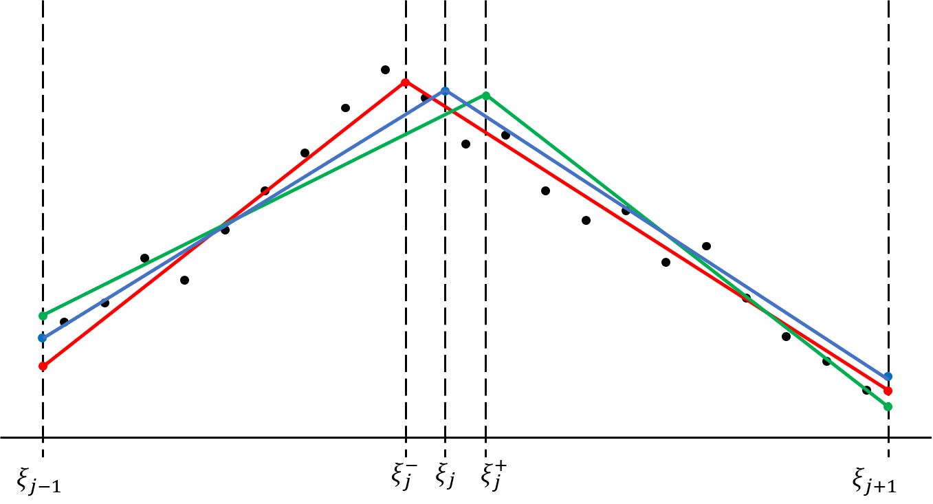
Figure 1: Update breakpoints among $\xi_{j}^{-},\xi_{j},\xi_{j}^{+}$.

3.1 Update breakpoints

Given the initial breakpoints $\xi_{1}^{(1)}<\xi_{2}^{(1)}<\ldots<\xi_{k-1}^{(1)}$, iteratively update breakpoints. After $t$ number of iterations, the breakpoints are denoted by

$$\xi_{1}^{(t)}<\cdots<\xi_{j-1}^{(t)}<\xi_{j}^{(t)}<\xi_{j+1}^{(t)}<\cdots<\xi_{k-1}^{(t)}.$$

We will explain the process of updating single breakpoint. For fixed $j$ and breakpoint $\xi_{j}^{(t)}$, consider three consecutive breakpoints $\xi_{j-1}^{(t)},\xi_{j}^{(t)},\xi_{j+1}^{(t)}$. Then there exist two disjoint subintervals $I_{j}=[\xi_{j-1}^{(t)},\xi_{j}^{(t)}]$, $I_{j+1}=[\xi_{j}^{(t)},\xi_{j+1}^{(t)}]$. Denote all elements $x_{i}$ in $I_{j}$ and $I_{j+1}$ respectively as

$$z_{1,j} <z_{2,j}<\cdots<z_{m_{j}-1,j}<z_{m_{j},j},$$

$$z_{1,j+1} <z_{2,j+1}<\cdots<z_{m_{j+1}-1,j+1}<z_{m_{j+1},j+1},$$

where $m_{j}$ is the total number of all $x_{i}$ in the subinterval $I_{j}$.

The candidate of breakpoints $\xi_{j}^{-}<\xi_{j}^{(t)}<\xi_{j}^{+}$ can be positioned as follows:

$$\begin{cases}\xi_{j}^{-}:=\cfrac{z_{m_{j}-1,j}+z_{m_{j},j}}{2},\\ \xi_{j}^{(t)}:=\cfrac{z_{m_{j},j}+z_{1,j+1}}{2},\\ \xi_{j}^{+}:=\cfrac{z_{1,j+1}+z_{2,j+1}}{2},\end{cases}$$

Function Update_BP 

       Input : $(\bm{x}_{\{j,j+1\}},\bm{y}_{\{j,j+1\}})\in\mathbb{R}^{(m_{j}+m_{j+1})\times 2}$: data; $[\xi_{j-1}^{(t)},\xi_{j}^{(t)},\xi_{j+1}^{(t)}]\in\mathbb{R}^{3}$: breakpoints; $d\in\mathbb{N}$: degree

       Output : $\xi_{j}^{(t+1)}\in\mathbb{R}$: updated breakpoint

       Create $\bm{V}_{j}^{-},\bm{V}_{j},\bm{V}_{j}^{+}$ from $\bm{x}_{\{j,j+1\}}$

       $\bm{\theta}^{-}_{j}$ $\leftarrow$ Solve (3.3)

       $\bm{\theta}^{(t)}_{j}$ $\leftarrow$ Solve (3.4)

       $\bm{\theta}^{+}_{j}$ $\leftarrow$ Solve (3.5)

       $r_{-}$ $\leftarrow$ $\operatorname{MSE}(\bm{X}_{j}^{-}\bm{\theta}^{-}_{j},\bm{y}_{\{j,j+1\}})$

       $r$ $\leftarrow$ $\operatorname{MSE}(\bm{X}_{j}\bm{\theta}^{(t)}_{j},\bm{y}_{\{j,j+1\}})$

       $r_{+}$ $\leftarrow$ $\operatorname{MSE}(\bm{X}_{j}^{+}\bm{\theta}^{+}_{j},\bm{y}_{\{j,j+1\}})$

       if $r_{-}<r~{}\mathbf{and}~{}r_{-}<r_{+}$ then

             $\xi_{j}^{(t+1)}$ $\leftarrow$ $\xi_{j}^{-}$ ;

            

       else if $r_{+}<r_{-}~{}\mathbf{and}~{}r_{+}<r$ then

             $\xi_{j}^{(t+1)}$ $\leftarrow$ $\xi_{j}^{+}$ ;

            

       else

             $\xi_{j}^{(t+1)}$ $\leftarrow$ $\xi_{j}^{(t)}$ ;

            

       end if

      

end

Algorithm 2 Update a single breakpoint

Update $\xi_{j}^{(t+1)}$ with the best of $\xi_{j}^{-},\xi_{j}^{(t)},\xi_{j}^{+}$which produces the regression with the smallest MSE (see Figure 1). To find the best breakpoint $\xi_{j}^{(t+1)}$, it needs to solve three optimization problems.

$$\mathscr{P}_{-}:{} \operatorname*{minimize}_{\bm{\theta}^{-}_{j}}\left\|\bm{X}_{j}^{-}\bm{\theta}^{-}_{j}-\bm{y}_{\{j,j+1\}}\right\|_{2}^{2}$$ (3.3)

$$\text{subject to }\begin{bmatrix}\bm{v}(\xi_{j}^{-})^{T}&-\bm{v}(\xi_{j}^{-})^{T}\end{bmatrix}\bm{\theta}^{-}_{j}=0,$$

$$\mathscr{P}_{0}:{} \operatorname*{minimize}_{\bm{\theta}^{(t)}_{j}}\left\|\bm{X}_{j}\bm{\theta}^{(t)}_{j}-\bm{y}_{\{j,j+1\}}\right\|_{2}^{2}$$ (3.4)

$$\text{subject to }\begin{bmatrix}\bm{v}(\xi_{j}^{(t)})^{T}&-\bm{v}(\xi_{j}^{(t)})^{T}\end{bmatrix}\bm{\theta}_{j}=0,$$

$$\mathscr{P}_{+}:{} \operatorname*{minimize}_{\bm{\theta}^{+}_{j}}\left\|\bm{X}_{j}^{+}\bm{\theta}^{+}_{j}-\bm{y}_{\{j,j+1\}}\right\|_{2}^{2}$$ (3.5)

$$\text{subject to }\begin{bmatrix}\bm{v}(\xi_{j}^{+})^{T}&-\bm{v}(\xi_{j}^{+})^{T}\end{bmatrix}\bm{\theta}^{+}_{j}=0,$$

where

$$\bm{X}_{j}^{-}= \begin{bmatrix}\bm{V}\left([\xi_{j-1}^{(t)},\xi_{j}^{-}]\right)&\\ &\bm{V}\left([\xi_{j}^{-},\xi_{j+1}^{(t)}]\right)\end{bmatrix},$$

$$\bm{X}_{j}= \begin{bmatrix}\bm{V}\left([\xi_{j-1}^{(t)},\xi_{j}^{(t)}]\right)&\\ &\bm{V}\left([\xi_{j},\xi_{j+1}^{(t)}]\right)\end{bmatrix},$$

$$\bm{X}_{j}^{+}= \begin{bmatrix}\bm{V}\left([\xi_{j-1}^{(t)},\xi_{j}^{+}]\right)&\\ &\bm{V}\left([\xi_{j}^{+},\xi_{j+1}^{(t)}]\right)\end{bmatrix},$$

$\bm{V}(I)$ is the Vandermonde matrix of the interval $I$ defined in (2.2) and $\bm{y}_{\{j,j+1\}}$ is the data of $x_{i}$ in $I_{j}$.

The breakpoint $\xi_{j}^{(t)}$ can be updated as:

$$\xi_{j}^{(t+1)}=\begin{cases}\xi_{j}^{-}&\text{if }r_{-}<r\text{ and }r_{-}<r_{+},\\ \xi_{j}^{(t)}&\text{if }r\leq r_{-}\text{ and }r\leq r_{+},\\ \xi_{j}^{+}&\text{if }r_{+}<r\text{ and }r_{+}<r_{-},\end{cases}$$

where $r_{-}=\operatorname{MSE}(\bm{X}_{j}^{-}\bm{\theta}^{-}_{j},\bm{y}_{\{j,j+1\}})$, $r=\operatorname{MSE}(\bm{X}_{j}^{(t)}\bm{\theta}^{(t)}_{j},\bm{y}_{\{j,j+1\}})$, $r_{+}=\operatorname{MSE}(\bm{X}_{j}^{+}\bm{\theta}^{+}_{j},\bm{y}_{\{j,j+1\}})$ (see Algorithm 2).

Function Find_BP 

       Input : $(\bm{x},\bm{y})\in\mathbb{R}^{n\times 2}$: data; $\bm{\xi}^{(0)}\in\mathbb{R}^{k+1}$: initial breakpoints; $d\in\mathbb{N}$: degree

       Output : $\hat{\bm{y}}\in\mathbb{R}^{n}$: piecewise regression; $\hat{\bm{\xi}}\in\mathbb{R}^{k}$: updated breakpoints

       $t$ $\leftarrow$ 0

       $\hat{\bm{y}}$ $\leftarrow$ Piecewise_regression​ $(\bm{x},\bm{y},\bm{\xi}^{(t)},d)$

            

      

      $error$ $\leftarrow$ $\operatorname{MSE}\left(\bm{\hat{y}},\bm{y}\right)$

       while stopping criteria not met do

             for $j\leftarrow 1$ to $k-1$ do

                   $\bm{x}_{\{j,j+1\}}$ $\leftarrow$ $\bm{x}(\bm{x}\geq\xi^{(t)}_{j-1}\,\,\,\&\,\,\,\bm{x}<\xi^{(t)}_{j+1})$

                   $\bm{y}_{\{j,j+1\}}$ $\leftarrow$ $\bm{y}(\bm{x}\geq\xi^{(t)}_{j-1}\,\,\,\&\,\,\,\bm{x}<\xi^{(t)}_{j+1})$

                   $\xi^{(t+1)}_{j}$ $\leftarrow$ Update_BP​ $(\bm{x}_{\{j,j+1\}},\bm{y}_{\{j,j+1\}},$

                          $[\xi^{(t)}_{j-1},\xi^{(t)}_{j},\xi^{(t)}_{j+1}],d)$

                        

                  

                  

             end for

            $\bm{\xi}^{(t+1)}$ $\leftarrow$ $[\xi_{0},\xi^{(t+1)}_{1},\xi^{(t+1)}_{2},\ldots,\xi^{(t+1)}_{k-1},\xi_{k}]$

             $\hat{\bm{y}}$ $\leftarrow$ Piecewise_regression​ $(\bm{x},\bm{y},\bm{\xi}^{(t+1)},d)$

                  

            

            if $\operatorname{MSE}\left(\bm{\hat{y}},\bm{y}\right)<error$ then

                   $error$ $\leftarrow$ $\operatorname{MSE}\left(\bm{\hat{y}},\bm{y}\right)$

                   $\hat{\bm{\xi}}$ $\leftarrow$ $\bm{\xi}^{(t+1)}$ ;

                  

             $t$ $\leftarrow$ $t+1$

            

       end while

      $\hat{\bm{y}}$ $\leftarrow$ Piecewise_regression​ $(\bm{x},\bm{y},\hat{\bm{\xi}},d)$

            

      

      

end

Algorithm 3 Find the optimal location of breakpoints

Funtion Optimal_BP 

       Input : $(\bm{x},\bm{y})\in\mathbb{R}^{n\times 2}$: data; $\bm{\xi}\in\mathbb{R}^{k+1}$: initial breakpoints; $d\in\mathbb{N}$: degree;

      $\tau\geq 1$: threshold for ratio of MSE;

       $p\in\mathbb{N}$: threshold for # of breakpoints

       Output : $\check{\bm{\xi}}$: optimal breakpoints

       while stopping criteria not met do

             $[\hat{\bm{y}},\hat{\bm{\xi}}]$ $\leftarrow$ Find_BP​ $(\bm{x},\bm{y},\bm{\xi},d)$

                  

            

            

            $\min\leftarrow\infty$

            

            for $j\leftarrow 1$ to $\operatorname{length}(\hat{\bm{\xi}})-1$ do

                   $\bm{\zeta}_{j}\leftarrow$Remove $\hat{\xi}_{j}$ from $\hat{\bm{\xi}}$

                   $\tilde{\bm{y}}$ $\leftarrow$ Piecewise_regression​ $(\bm{x},\bm{y},\bm{\zeta}_{j},d)$

                        

                  

                  $\text{loss}_{j}$ $\leftarrow$ $\cfrac{\operatorname{MSE}\left(\bm{\tilde{y}},\bm{y}\right)}{\operatorname{MSE}\left(\hat{\bm{y}},\bm{y}\right)}$

                   if $\text{loss}_{j}\leq\min$ then

                         $\min\leftarrow\text{loss}_{j}$

                         $\tilde{\bm{\xi}}\leftarrow\bm{\zeta}_{j}$

                   end if

                  

             end for

            $\bm{\xi}\leftarrow\tilde{\bm{\xi}}$

       end while

      $\check{\bm{\xi}}\leftarrow\hat{\bm{\xi}}$

      

end

Algorithm 4 Find the optimal number of breakpoints

Note that Algorithm 2 updates only a single breakpoint. To update all breakpoints, the algorithm repeats this process consecutively for $j=1,2,\ldots,k-1$. The first $\xi_{0}$ and the last $\xi_{k}$ are not updated for any iteration. For each iteration, the breakpoints $\xi_{1}^{(t)},\ldots,\xi_{k-1}^{(t)}$ are updated independently. This means that the updated $\xi_{j}^{(t+1)}$ has no effect on the updating process of $\xi_{1}^{(t)},\ldots,\xi_{j-1}^{(t)},\xi_{j+1}^{(t)}\ldots,\xi_{k-1}^{(t)}$. The initial breakpoints are chosen randomly or heuristically. There are two criteria under which Algorithm 3 terminates. The first is when all breakpoints are no longer updated, and the second is when an updated breakpoint appeared in the previous iteration (see Algorithm 3).

The main computational complexity of Algorithm 2 lies in solving optimization problems (3.3) through (3.5). Each optimization problem within a subinterval can be addressed using Algorithm 2, which involves computing the inverse of a $(2d+3)\times(2d+3)$ matrix as described in (2.4), where $d$ is the polynomial degree. In particular, for piecewise linear regression, each optimization problem becomes the problem of finding the inverse of a matrix of size $5\times 5$, which is a very time-efficient problem. Moreover, parallel computation technique can be applied since the updated breakpoint $\xi^{(t+1)}_{j}$ for the $j$-th breakpoint $\xi^{(t)}_{j}$ in the $t$-th iteration is not reflected in the update of the ($j+1$)-th breakpoint $\xi^{(t)}_{j+1}$ in the $t$-th iteration.

3.2 Finding the optimal number of breakpoints

In this section, we propose an algorithm to determine the optimal breakpoints for piecewise polynomial regression. The optimal number of breakpoints is crucial for accurately modeling and interpreting the data. The number of breakpoints is closely related to the under-fitting and over-fitting of piecewise regression models. Too few breakpoints can lead to a model that misses important trend changes, while too many can result in a model that is overly complex and sensitive to random fluctuations in the data [17]. By finding the optimal number of breakpoints, a balance can be achieved that provides meaningful insights and maintains the generalizability of the model.

Similarly to other iteration-based algorithms for nonconvex optimization, Algorithm 3 may possibly converge to a local minimum depending on the initial value (see Figure 3.(a)). To avoid this situation, Algorithm 4 starts with a sufficiently large number of breakpoints and then removes the most redundant breakpoint in the sense of optimization.

Specifically, assume that breakpoints $\bm{\xi}=[\xi_{0}~{}\xi_{1}~{}\cdots~{}\xi_{k}]^{T}$ with endpoints $\xi_{0}$, $\xi_{k}$ are found by Algorithm 3. Consider the following $k-1$ optimization problems for $i=1,2,\ldots,k-1$. This optimization problem is equivalent to piecewise polynomial regression in the absence of the $i$-th breakpoint in $\bm{\xi}$. And then select the most redundant breakpoint $\xi_{i}$, which has the smallest MSE among the optimization problems $\mathscr{P}_{i}$.

$$\mathscr{P}_{i}:{} \operatorname*{minimize}_{\bm{\theta}_{i}}\left\|\bm{X}_{i}\bm{\theta}_{i}-\bm{y}\right\|_{2}^{2}$$ (3.6)

$$\text{subject to }\bm{C}_{i}\bm{\theta}_{i}=\bm{0}$$

where

$$\bm{X}_{i} =\begin{bmatrix}\bm{V}(I_{1})&&\cdots&&\bm{0}\\ &\ddots&&&\\ \vdots&&\bm{V}(I_{i-1}\cup I_{i})&&\vdots\\ &&&\ddots&\\ \bm{0}&&\cdots&&\bm{V}(I_{k})\end{bmatrix},$$

$$\bm{C}_{\bm{\zeta}_{i}} =\begin{bmatrix}\bm{v}(\xi_{1})&\\ -\bm{v}(\xi_{1})&\ddots&\\ &\ddots&\bm{v}(\xi_{i-1})&\\ &&-\bm{v}(\xi_{i-1})&\bm{v}(\xi_{i+1})&\\ &&&-\bm{v}(\xi_{i+1})&\ddots&\\ &&&&\ddots&\bm{v}(\xi_{k-1})&\\ &&&&&-\bm{v}(\xi_{k-1})\end{bmatrix}^{T},$$

$$\bm{\zeta}_{i} =\begin{bmatrix}\xi_{0}&\xi_{1}&\cdots&\xi_{i-1}&\xi_{i+1}&\cdots&\xi_{k-1}&\xi_{k}\end{bmatrix}^{T}.$$

To determine which breakpoints to remove, let $\bm{\theta}$ be a solution of the optimization problem (2.3) with breakpoint $\bm{\xi}$. Consider following set:

$$\mathcal{S}=\left\{\frac{\operatorname{MSE}(\bm{X}_{i}\bm{\theta}_{i},\bm{y})}{\operatorname{MSE}(\bm{X}\bm{\theta},\bm{y})}\Big{|}\bm{\theta}_{i}:\text{optimal solution of }\mathscr{P}_{i}\right\}.$$

Then the elements of $\mathcal{S}$ represent the ratio of MSE for the piecewise regression models before and after removal of the breakpoint $\xi_{i}$. The breakpoint $\xi_{i}$ which minimizes $\mathcal{S}$ represents that it has the least impact on the results of the piecewise regression. If $\min{\mathcal{S}}$ is sufficiently large, this indicates that removing any breakpoints significantly affects the piecewise regression, suggesting that all breakpoints are critical to the model. For $\bm{\zeta}_{i}=[\xi_{0},~{}\xi_{1},~{}\cdots,~{}\xi_{i-1},~{}\xi_{i+1},~{}\cdots,~{}\xi_{k-1},~{}\xi_{k}]^{T}$, update $\bm{\zeta}_{i}$ to its optimal location using Algorithm 3, and then set it as the new $\bm{\xi}$. This process is repeated until the stopping criterion is met (see Algorithm 4).

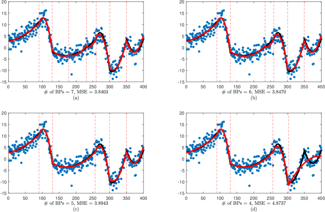
Figure 2: Comparing MSE as the number of breakpoints is reduced from $7$ to $4$.

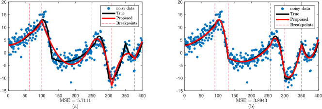
Figure 3: Algorithm 4 can avoid local minimum well.

There are two stopping criterion for Algorithm 4. The first stopping criterion is the tolerance $\tau\geq 1$, which represents the percentage increase allowed in MSE when a breakpoint is removed. If the minimum percentage increases $\min{\mathcal{S}}>\tau$, then $\bm{\xi}$ is deemed the optimal set of breakpoints before considering any removals. The tolerance $\tau$ controls the balance between overfitting and underfitting in piecewise regression. A higher value of $\tau$ implies a wider tolerance range, leading to the removal of more breakpoints, which can result in underfitting. On the other hand, a lower $\tau$ indicates a narrower tolerance range, leading to the retention of more breakpoints, thereby increasing the risk of overfitting. Therefore, selecting an appropriate value of $\tau$ is crucial and should be based on the characteristics of the data.

The second criterion is the tolerance $p\in\mathbb{N}$, representing the maximum allowed number of breakpoints. The process of removing breakpoints is repeated until the number of breakpoints is equal to or less than $p$. This criterion is particularly effective when prior knowledge about the data suggests a specific number of breakpoints.

For example, the MSE of the piecewise regression using Algorithm 4, starting with $7$ breakpoints and reducing the breakpoints by one, is shown in Figure 2. The MSE increases very slightly when there were enough breakpoints by eliminating inconsequential breakpoints, but it increase dramatically from $3.8943$ to $4.8737$ when the number of breakpoints was reduced from $5$ to $4$. The algorithm stops and concludes that $5$ is the optimal number of breakpoints if reducing the breakpoints causes the MSE to rise noticeably.

Furthermore, Figure 3 shows the effectiveness of the proposed Algorithm 4. Figure 3.(a) is the result of Algorithm 3 for five randomly generated initial breakpoints $\xi_{1}=69.5,\xi_{2}=99.5,\xi_{3}=239.5,\xi_{4}=319.5,\xi_{5}=369.5$. The MSE is $5.7111$, indicating that the piecewise regression reaches a local minimum and does not fit the data well. However, the MSE of the regression in Figure 3.(b), which is the result of Algorithm 4, is $3.8943$, effectively avoiding the local minimum. This even has a lower MSE than the true piecewise quadratic model before adding noise, which has an MSE of $4.0988$, represented by the solid black line.

4 Experimental Results

In this section, numerical experiments with some synthetic and real data are presented to show the effectiveness of our proposed algorithm. Every numerical experiment uses Matlab and the tests were executed on a high-performance computing system with the following specifications: an AMD Ryzen 3970X CPU running at 3.69 GHz.

4.1 Synthetic data

In this section, we compare the proposed method with several regression methods with synthetic data $\{(x_{i},y_{i})\}_{i=1}^{n}\subset\mathbb{R}^{2}$. The benchmark methods are as follows:

Polynomial Regression (PR)
In a polynomial regression model [26], a polynomial of degree $d$ is fit to given data. The goal is to minimize the difference between the predicted value and the actual value for each data point.

$$\operatorname*{minimize}_{\bm{\beta}}\sum_{i=1}^{n}\left(y_{i}-\sum_{j=0}^{d}\beta_{j}x_{i}^{j}\right)^{2}$$ (4.1)

Spline Regression (SR)
A spline model is a combination of polynomials that smoothly connects data points. The optimization problem minimizes the sum of the squared errors at the data points, while simultaneously minimizing the integral of the square of the second derivative to maintain the smoothness of the spline. Here, $\lambda$ controls the trade-off between smoothness and data fit.

$$\operatorname*{minimize}_{f}p\sum_{i=1}^{n}w_{i}\left|y_{i}-f\left(x_{i}\right)\right|^{2}+(1-p)\int\lambda(t)\left|D^{2}f(t)\right|^{2}dt$$ (4.2)

Support Vector Regression (SVR)
Support vector regression [25] is a regression method that aims to ensure as many data points as possible are within an $\epsilon$-tube. Let $\phi$ be a kernel function that maps the input data to a high-dimensional feature space. The $\psi_{i}$ and $\hat{\psi}_{i}$ ($i=1,\ldots n$) are slack variables that allow for errors for data points outside the $\epsilon$-tube.

$$\operatorname*{minimize}_{w,b,\psi,\hat{\psi}} \frac{1}{2}|w|^{2}+\lambda\sum_{i=1}^{n}(\psi_{i}+\hat{\psi}_{i})$$ (4.3)

subject to $$y_{i}-(w\phi(x_{i})+b)\leq\epsilon+\psi_{i},$$

$$(w\phi(x_{i})+b)-y_{i}\leq\epsilon+\hat{\psi}_{i},$$

$$\psi_{i},\hat{\psi}_{i}\geq 0,$$

where $\lambda$ is a trade-off parameter trade-off between the flatness of model and the amount up to which deviations larger than $\epsilon$ are tolerated.

Decision Tree Regression (DT)
In decision tree regression [21], the data space is partitioned into multiple bins $R_{m}$, and the mean value $\bar{y}_{R_{m}}$ within each bin is used as the predicted value. The optimization problem is to minimize the sum of squared errors within these bins.

$$\operatorname*{minimize}_{T}\sum_{m=1}^{M}\sum_{i\in R_{m}}(y_{i}-\bar{y}_{R_{m}})^{2}$$ (4.4)

Gradient Boosting Regression (GB)
In gradient boosting regression [11], the model $F_{0}$ is initially set to the mean of the target variable $y$, expressed as $F_{0}(x)=\bar{y}$. At each iteration $m$, the residuals $r_{i}^{(m)}$ are calculated based on the difference between the actual target values $y_{i}$ and the predictions from the current ensemble model $F_{m-1}$. This is given by $r_{i}^{(m)}=y_{i}-F_{m-1}(x_{i})$. A weak learner $h_{m}$ is then trained to predict these residuals by minimizing the sum of squared errors for the residuals:

$$h_{m}=\arg\min_{h}\sum_{i=1}^{N}(r_{i}^{(m)}-h(x_{i}))^{2}.$$

After $M$ iterations, the final model is expressed as:

$$F_{M}(x)=F_{0}(x)+\sum_{m=1}^{M}\nu\cdot h_{m}(x).$$

Here, $\nu$ is a parameter that controls the contribution of each weak learner, helping to prevent overfitting by ensuring that the updates are gradual.

Random Forest Regression (RF)
In random forest regression [5], multiple decision trees are trained on different subsets of the data, and their predictions are averaged to produce a final output. This method reduces overfitting and improves the model’s generalization by leveraging the diversity among the trees.

$$\operatorname*{minimize}_{f}\sum_{i=1}^{n}\left(y_{i}-\hat{y}_{i}\right)^{2},\quad\text{where}\quad\hat{y}_{i}=\frac{1}{T}\sum_{t=1}^{T}h_{t}(x_{i})$$

Here, $f$ is random forest regression prediction function, given data $\{(x_{i},y_{i})\}_{i=1}^{n}\subset\mathbb{R}^{2}$, $\hat{y}_{i}$ is the predicted value for data point $i$, $T$ is the number of learning cycles, and $h_{t}(x_{i})$ is the prediction of the $t$-th decision tree learner for $x_{i}$.

$\bm{\ell_{1}}$ Trend Filter
$\ell_{1}$ trend filter [19] detects trends in data while avoiding sharp changes in trend. It does this by penalizing the sum of the absolute values of the trend changes while minimizing the absolute value of the error.

$$\operatorname*{minimize}_{\hat{\bm{y}}}\frac{1}{2}\|\bm{y}-\hat{\bm{y}}\|_{2}^{2}+\|\bm{D}\hat{\bm{y}}\|_{1},$$ (4.5)

where $\bm{y}=[y_{1},\ldots,y_{n}]^{T}$ is given data, $\hat{\bm{y}}=[\hat{y}_{1},\ldots,\hat{y}_{n}]^{T}$ is predicted value and $\bm{D}$ is the second-order difference matrix, i.e,

$$D=\begin{bmatrix}1&-2&1&&&&\\ &1&-2&1&&&\\ &&\ddots&\ddots&\ddots&&\\ &&&1&-2&1&\\ &&&&1&-2&1\end{bmatrix}\in\mathbb{R}^{(n-2)\times n}.$$

Adaptive Piecewise Linear Regression (APLR)
Adaptive piecewise linear regression [17] fits linear models to segments of the data. The optimization problem is to minimize the sum of squared errors within each segment while ensuring continuity at the segment boundaries. Let

$$F(\bm{\xi})=\sum_{j=1}^{k}\sum_{x_{i}\in I_{j}}\left(p_{j}^{d}\left(x_{i}\right)-y_{i}\right)^{2}.$$

$$\operatorname{minimize}F(\bm{\xi})$$ (4.6)

$$\text{subject to }p_{j}^{d}\left(\xi_{j}\right)=p_{j+1}^{d}\left(\xi_{j}\right),j=1,\ldots,k-1$$

Then the breakpoints $\bm{\xi}$ is updated as follows:

$$\bm{\xi}=\bm{\xi}-\mu\nabla F\left(\bm{\xi}\right).$$

Here, $\mu$ is gradient descent step.

Pruned Exact Linear Time (PELT)
The pruned exact linear time algorithm [18] detects changes in data points, divides them into regions, and applies a linear model to each region. The optimization problem controls the complexity of the model by assigning a penalty $\beta$ to the number of change points $k$ while minimizing the overall cost function.

$$\operatorname*{minimize}_{{t_{1},t_{2},\dots,t_{k}}}\left(\sum_{j=1}^{k+1}\sum_{i=t_{j-1}}^{t_{j}-1}(y_{i}-\hat{y}_{i})^{2}+k\beta\right)$$ (4.7)

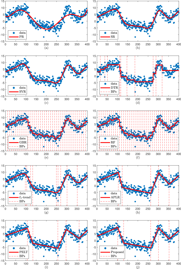
Figure 4: Result of each regression models.

In particular, $\mathtt{ischange}$ function, built-in function of Matlab for detecting trend change points is based on this algorithm.

To generate synthetic data $\{(x_{i},y_{i})\}_{1\leq i\leq 400}$ randomly, there are two processes: (i) generate a piecewise linear function $f$ with $\bm{\xi}=[1,70,150,230,300,350,400]^{T}$ and randomly generated values $f(\xi_{i})\sim\mathcal{U}\{-15,15\}$. Here, $\mathcal{U}$ presents a discrete uniform distribution. The value of $y_{i}$ at fixed $x_{i}=i$ is randomly generated by $y_{i}=f(x_{i})+\epsilon_{i}$ with noise $\epsilon_{i}\sim\mathcal{N}(0,2)$.

The following evaluation metrics are introduced to compare the performance of the algorithm: mean square error (MSE), mean absolute error (MAE), relative absolute error (RAE), coefficient of determination ($R^{2}$) and number of breakpoints (BPs). These metrics were used to compare the performance of different algorithms.

$$\operatorname{MSE}(\bm{y},\hat{\bm{y}}) =\frac{1}{n}\sum_{i=1}^{n}(y_{i}-\hat{y}_{i})^{2}$$

$$\operatorname{RMSE}(\bm{y},\hat{\bm{y}}) =\sqrt{\operatorname{MSE}(\bm{y},\hat{\bm{y}})}$$

$$\operatorname{MAE}(\bm{y},\hat{\bm{y}}) =\frac{1}{n}\sum\limits_{i=1}^{n}|y_{i}-\hat{y}_{i}|$$

$$\operatorname{RAE}(\bm{y},\hat{\bm{y}}) =\frac{\sum\limits_{i=1}^{n}|y_{i}-\hat{y}_{i}|}{\sum\limits_{i=1}^{n}|y_{i}-\bar{\bm{y}}|}$$

$$R^{2} =1-\frac{\sum\limits_{i=1}^{n}|\hat{y}_{i}-\bar{\bm{y}}|}{\sum\limits_{i=1}^{n}(y_{i}-\bar{\bm{y}})^{2}}$$

$$\operatorname{BPs} =\textrm{number of breakpoints}$$

Here, $\bar{\bm{y}}$ presents the average of $\bm{y}=[y_{1},\ldots,y_{n}]^{T}$, i.e., $\bar{\bm{y}}=\frac{1}{n}\sum_{i=1}^{n}y_{i}$.

Note that the number of breakpoints is a significant factor in determining the balance between model complexity and the ability to capture the underlying trends. A higher number of breakpoints can indicate overfitting, where the model is too closely tailored to the training data, potentially compromising its generalization to new data. In contrast, too few breakpoints might result in a model that cannot adequately capture the trend within the data.

Model	MAE	RAE	MSE	$\bm{R^{2}}$	BPs
PR	2.1924	0.4837	7.5856	0.7200	0
SR	1.5716	0.3468	4.0950	0.8489	0
SVR	1.5857	0.3499	4.2108	0.8446	0
DT	1.6739	0.3693	4.5007	0.8339	10
GB	1.5586	0.3439	3.9687	0.8535	39
RF	1.5621	0.3447	4.0066	0.8521	39
$\ell_{1}$ trend	1.6146	0.3562	4.3264	0.8403	8
APLR	$\bm{1.5368}$	$\bm{0.3391}$	3.9545	0.8541	$\bm{5}$
PELT	1.6282	0.3592	4.4442	0.8360	$\bm{5}$
Proposed	1.5387	0.3395	$\bm{3.9428}$	$\bm{0.8545}$	$\bm{5}$

Table 1: Comparison of different regression models (Metrics from Figure 4).

Table 1 compares various piecewise regression methods based on several performance metrics: MAE, RAE, MSE, $R^{2}$ and BPs. In evaluating these metrics, a few critical points emerge. The result of the proposed method in Table 1 shows remarkable performance in several metrics. It achieves the highest $R^{2}$ value of 0.8545, indicating a strong fit to the data. In addition, it shows the lowest MSE and RAE, which are crucial indicators of model accuracy and reliability. These low error rates suggest that the proposed method not only fits the training data well but also maintains a robust prediction accuracy. One of the most notable aspects of the proposed method is its balance in the number of breakpoints. The proposed method has only 5 breakpoints, it avoids the pitfall of overfitting methods like DT and RF exhibit, which use 10 and 39 breakpoints, respectively. At the same time, it overcomes the limitation of methods like Polynomial and Spline, which use no breakpoints and may fail to capture the underlying trend accurately (see Figure 4).

This balance highlights the strength of the proposed method in providing a more flexible approach to piecewise regression. It leverages a sufficient number of breakpoints to model complexity of data without succumbing to overfitting, thereby presenting a more reliable and generalizable model. This makes the proposed method a superior choice compared to others, achieving an optimal trade-off between capturing data trends and maintaining model simplicity.

4.2 Real data

A linear regression may not be a proper model for real data. Rather, piecewise linear regression can provide the flexibility to capture abrupt changes or trend changes at specific points in the data. In this section, the proposed method is applied to a variety of real-world data and compared with the results of other piecewise regression methods. financial real dataset and epidemic real dataset are considered.

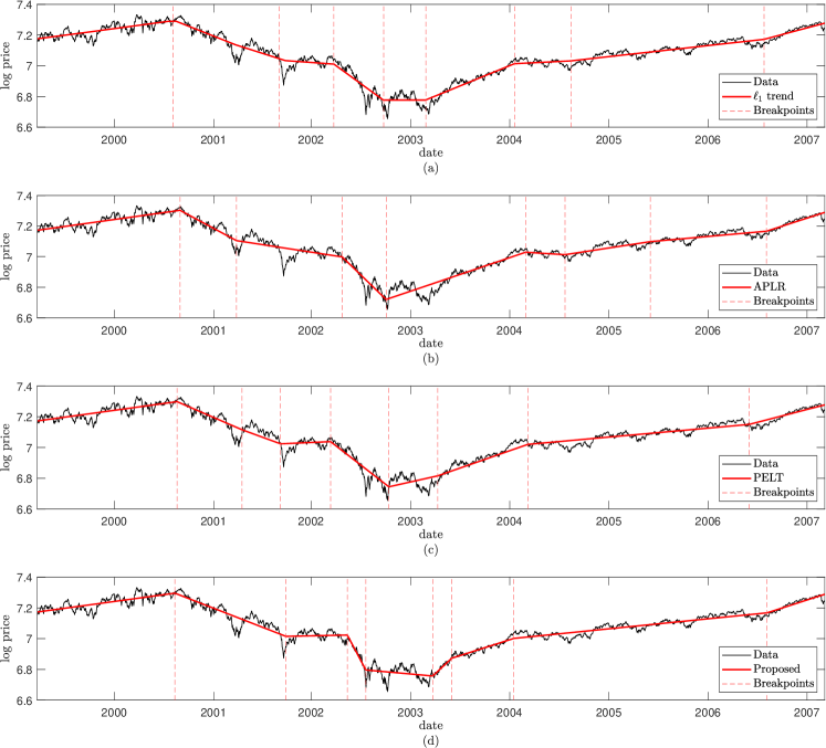
Figure 5: Comparison of $\ell_{1}$ trend filter, APLR, PELT and proposed method for S&P 500 data.

S&P 500 index data

S&P 500 index data is the most representative and widely traded indices in their respective markets, namely the New York Stock Exchange. The dataset is generated every business day from March 25, 1999, to March 9, 2007, and regression is performed on the logarithm of the adjusted closing price. The logarithm transformation is widely used in financial analysis to stabilize variance and make data more suitable for certain statistical modeling.

In the previous synthetic experiment, it is observed that $\ell_{1}$ trend filter, APLR, PELT, and the proposed method estimate the trend of the data with a small number of breakpoints. Therefore, let us compare the results of the piecewise regression of these three methods. Set the parameter $\gamma=100$ for $\ell_{1}$ trend filter. The number of breakpoints for APLR and PELT is set to 10 using the heuristic approach, and the number of initial breakpoints for Algorithm 4 was set to 15.

Model	MAE	RAE	RMSE	$\bm{R^{2}}$	BPs
$\ell_{1}$ trend	0.0239	0.2018	0.0314	0.9548	8
APLR	0.0242	0.2041	0.0327	0.9509	8
PELT	0.0257	0.2169	0.0332	0.9496	8
Proposed	$\bm{0.0228}$	$\bm{0.1921}$	$\bm{0.0299}$	$\bm{0.9592}$	$\bm{8}$

Table 2: Performance comparison of $\ell_{1}$ trend filter, APLR, PELT, proposed method for S&P 500 data (see Figure 5).

Table 2 presents a performance comparison of four methods: $\ell_{1}$ trend filter, APLR, PELT, and a proposed method evaluated on S&P 500 data across MAE, RAE, RMSE, $R^{2}$, and the number of breakpoints. All methods identify 8 breakpoints, ensuring comparability. The proposed method outperforms the others, achieving the lowest MAE (0.0228), RAE (0.1921), and RMSE (0.0299), along with the highest $R^{2}$ value (0.9592), indicating superior predictive precision and robustness. This shows the effectiveness of the proposed method in capturing the underlying trend in the data (see Figure 5).

COVID-19 case data

The second real-world dataset is the COVID-19 data provided by the Korea Disease Control and Prevention Agency (KDCA) [27] from January 20, 2020 to July 24, 2021. This period preceded the predominance of the delta variant of the COVID-19 virus, and the South Korean government implemented a phased approach to quarantine during this time, including social distancing and mandatory masks [20].

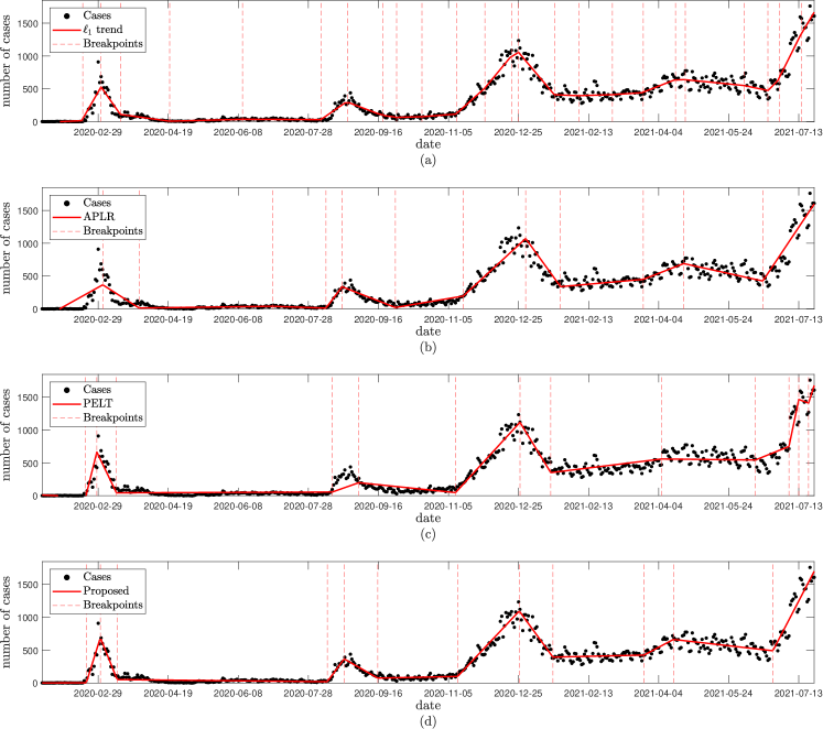
Figure 6: Comparison of $\ell_{1}$ trend filter, APLR, PELT and proposed method for COVID-19 cases dataset.

The regression is performed on the number of confirmed cases (real-time reverse transcription polymerase chain reaction test positive cases). $\ell_{1}$ trend filter, APLR, PELT, and the proposed method for the dataset are considered. The black dots represent daily cases, and the red line represents the regression model fitted to the data. The red dashed lines represent breakpoints where a change in trend is observed (see Figure 6).

Model	MAE	RAE	RMSE	$\bm{R^{2}}$	BPs
$\ell_{1}$ trend	46.6322	0.1696	71.6204	0.9557	24
APLR	60.8801	0.2214	92.4369	0.9262	12
PELT	63.4558	0.2308	88.4348	0.9325	13
Proposed	47.5149	0.1728	70.8662	0.9566	12

Table 3: Performance comparison of $\ell_{1}$ trend filter, APLR, PELT, proposed method for Korean COVID-19 data (see Figure 6).

Table 3 compares among the models using several metrics. Although $\ell_{1}$ trend filter achieves the lowest MAE and RAE, the proposed method exhibits the best RMSE and $R^{2}$ values, indicating a superior overall model performance in terms of fit to the data. And the proposed method also identifies fewer breakpoints which is 12, suggesting a more parsimonious model compared to $\ell_{1}$ trend filter, which identifies 24 breakpoints. This indicates that the proposed method effectively balances the trade-off between model complexity and fit quality. The ability of the model to follow the main trends without overfitting to short-term fluctuations is crucial to accurately capturing the dynamics of the pandemic.

5 Conclusion

In this study, we proposed a novel piecewise regression algorithm that effectively identifies breakpoints to minimize errors. Through numerical experiments using synthetic and real data, we show that the proposed method has high performance in piecewise polynomial regression. Furthermore, the algorithm can determine the optimal number of breakpoints.

In future work, the process of detecting breakpoints in piecewise regression should consider using reinforcement learning that takes into account long-term rewards. Although current algorithms focus on short-term gains and run the risk of converging to local minima, reinforcement learning may lead to more optimized results. This approach is expected to increase the accuracy and stability of models and improve their adaptability to different data types and robustness.

References

• Bai [1997] J. Bai. Estimation of a change point in multiple regression models. Review of Economics and Statistics, 79(4):551–563, 1997.
• Bai and Perron [1998] J. Bai and P. Perron. Estimating and testing linear models with multiple structural changes. Econometrica, pages 47–78, 1998.
• Bai and Perron [2003] J. Bai and P. Perron. Computation and analysis of multiple structural change models. Journal of applied econometrics, 18(1):1–22, 2003.
• Boyd and Vandenberghe [2018] S. Boyd and L. Vandenberghe. Introduction to applied linear algebra: vectors, matrices, and least squares. Cambridge university press, 2018.
• Breiman [2001] L. Breiman. Random forests. Machine learning, 45:5–32, 2001.
• Chiou et al. [2019] J.-M. Chiou, Y.-T. Chen, and T. Hsing. Identifying multiple changes for a functional data sequence with application to freeway traffic segmentation. The Annals of Applied Statistics, 13(3):1430–1463, 2019.
• Dell’Accio and Nudo [2024] F. Dell’Accio and F. Nudo. Polynomial approximation of derivatives through a regression–interpolation method. Applied Mathematics Letters, 152:109010, 2024.
• Dell’Accio et al. [2022] F. Dell’Accio, F. Di Tommaso, and F. Nudo. Generalizations of the constrained mock-chebyshev least squares in two variables: Tensor product vs total degree polynomial interpolation. Applied Mathematics Letters, 125:107732, 2022.
• Ding [2019] Y. Ding. Data science for wind energy. Chapman and Hall/CRC, 2019.
• Fearnhead and Liu [2007] P. Fearnhead and Z. Liu. On-line inference for multiple changepoint problems. Journal of the Royal Statistical Society Series B: Statistical Methodology, 69(4):589–605, 2007.
• Friedman [2001] J. H. Friedman. Greedy function approximation: a gradient boosting machine. Annals of statistics, pages 1189–1232, 2001.
• Fryzlewicz [2014] P. Fryzlewicz. Wild binary segmentation for multiple change-point detection. The Annals of Statistics, 42(6):2243–2281, 2014.
• Greene et al. [2015] M. Greene, O. Rolfson, G. Garellick, M. Gordon, and S. Nemes. Improved statistical analysis of pre-and post-treatment patient-reported outcome measures (proms): the applicability of piecewise linear regression splines. Quality of Life Research, 24:567–573, 2015.
• Guan et al. [2018] Y. Guan, K. Pan, and K. Zhou. Polynomial time algorithms and extended formulations for unit commitment problems. IISE transactions, 50(8):735–751, 2018.
• Gunnerud and Foss [2010] V. Gunnerud and B. Foss. Oil production optimization—a piecewise linear model, solved with two decomposition strategies. Computers & Chemical Engineering, 34(11):1803–1812, 2010.
• Hwangbo et al. [2018] H. Hwangbo, A. L. Johnson, and Y. Ding. Spline model for wake effect analysis: Characteristics of a single wake and its impacts on wind turbine power generation. IISE Transactions, 50(2):112–125, 2018.
• Jeong et al. [2023] J. Jeong, Y. M. Jung, S. H. Kim, and S. Yun. Trend filtering by adaptive piecewise polynomials. Communications in Nonlinear Science and Numerical Simulation, 116:106866, 2023.
• Killick et al. [2012] R. Killick, P. Fearnhead, and I. A. Eckley. Optimal detection of changepoints with a linear computational cost. Journal of the American Statistical Association, 107(500):1590–1598, 2012.
• Kim et al. [2009] S.-J. Kim, K. Koh, S. Boyd, and D. Gorinevsky. $\ell_{1}$ trend filtering. SIAM review, 51(2):339–360, 2009.
• Lee et al. [2022] H. Lee, G. Jang, and G. Cho. Forecasting covid-19 cases by assessing control-intervention effects in republic of korea: a statistical modeling approach. Alexandria Engineering Journal, 61(11):9203–9217, 2022.
• Loh [2011] W.-Y. Loh. Classification and regression trees. Wiley interdisciplinary reviews: data mining and knowledge discovery, 1(1):14–23, 2011.
• Muggeo [2003] V. M. Muggeo. Estimating regression models with unknown break-points. Statistics in medicine, 22(19):3055–3071, 2003.
• Muriel and Munshi [2004] A. Muriel and F. N. Munshi. Capacitated multicommodity network flow problems with piecewise linear concave costs. IIE Transactions, 36(7):683–696, 2004.
• Quarteroni et al. [2006] A. Quarteroni, R. Sacco, and F. Saleri. Numerical mathematics, volume 37. Springer Science & Business Media, 2006.
• Smola and Schölkopf [2004] A. J. Smola and B. Schölkopf. A tutorial on support vector regression. Statistics and computing, 14:199–222, 2004.
• Stigler [1971] S. M. Stigler. Optimal experimental design for polynomial regression. Journal of the American Statistical Association, 66(334):311–318, 1971.
• Korea Disease Control and Prevention Agency (2021) [KDCA] Korea Disease Control and Prevention Agency (KDCA). https://dportal.kdca.go.kr/pot/index.do, 2021. [accessed 18 June 2024].
• Tibshirani [2014] R. J. Tibshirani. Adaptive piecewise polynomial estimation via trend filtering. The Annals of Statistics, 42(1):285, 2014.
• Tomal and Rahman [2021] J. H. Tomal and H. Rahman. A bayesian piecewise linear model for the detection of breakpoints in housing prices. Metron, 79(3):361–381, 2021.
• Truong et al. [2020] C. Truong, L. Oudre, and N. Vayatis. Selective review of offline change point detection methods. Signal Processing, 167:107299, 2020.
• Tunc and Genç [2021] H. Tunc and B. Genç. A column generation based heuristic algorithm for piecewise linear regression. Expert Systems with Applications, 171:114539, 2021.
• Vieth [1989] E. Vieth. Fitting piecewise linear regression functions to biological responses. Journal of applied physiology, 67(1):390–396, 1989.
• Wagner et al. [2002] A. K. Wagner, S. B. Soumerai, F. Zhang, and D. Ross-Degnan. Segmented regression analysis of interrupted time series studies in medication use research. Journal of clinical pharmacy and therapeutics, 27(4):299–309, 2002.
• Wu et al. [2022] Z. Wu, Y. Li, and L. Hu. A synchronous multiple change-point detecting method for manufacturing process. Computers & Industrial Engineering, 169:108114, 2022.
• Yang et al. [2016] L. Yang, S. Liu, S. Tsoka, and L. G. Papageorgiou. Mathematical programming for piecewise linear regression analysis. Expert systems with applications, 44:156–167, 2016.