Resolving FLRW Cosmology Through Effective Equation of State in $f(T)$ Gravity

Abstract

Abstract: - This article explores the cosmological scenario of the universe in the context of the $f(T)$ power law model, where $T$ represents the torsion scalar. To obtain the deterministic solution of the field equations, we parametrized the effective Equation-of-State with two parameters $m$ and $k$ as suggested by A. Mukherjee in a flat FLRW environment. We impose constraints on the free parameters of the derived solution by utilizing MCMC analysis, assuming the $CC,Pantheon+SH0ES$, and $CC+Pantheon+SH0ES$ as data samples. We explore the dynamics of cosmological parameters. The evolutionary profile of the deceleration parameter exhibits the transition to the accelerated phase. The effective Equation-of-State parameter indicates the model remains in the quintessence era and gradually becomes the Einstein-de Sitter model. In addition to this, we also explore the jerk, snap, and lerk parameters. Furthermore, the $Om(z)$ diagnostic shows that the model has a consistent positive slope across the entire evolution, but soon resembles the standard $\Lambda$CDM model. At last, we conclude that the power law model of the $f(T)$ gravity in the framework of the FLRW universe aligns more closely with the $\Lambda$CDM model for given observational data.

Keywords: $f(T)$ gravity; Dark Energy; Equation-of-State; Observational Data.

I Introduction

A wide range of cosmological observations, such as the Type Ia Supernovae (SNeIa) [1], the cosmic microwave background radiation (CMBR) [2], the large-scale structure [3], and so forth, have demonstrated that the universe is expanding at an accelerated rate. This surprising observation of a phenomenon raises one of the most challenging issues in modern cosmology. It is commonly believed that an unidentified so-called dark energy (DE) is the primary gradient that causes the acceleration of the universe. This exotic energy component, characterized by negative pressure, influences the universe, filled with cold dark matter (CDM), and drives the recent acceleration of the universe’s expansion. Over the last ten years, many DE models like quintessence, phantom, k-essence, tachyon, quintom [4]; as well as the Chaplygin gas [5], the generalized Chaplygin gas (GCG) [6], the holographic DE [7], the new agegraphic DE [8], the Ricci DE [9] and so on have been suggested. The characteristics of DE are currently one of the most challenging issues in particle physics and modern cosmology. Approximately 75% of the total energy of the universe is thought to be covered by DE. The constant Equation-of-State (EoS) parameter $\omega\approx-1$ and, the vacuum energy (cosmological constant, $\Lambda$) are the most straightforward and appealing candidates for DE. It gets difficult to reconcile the small observational value of DE density that is coming from quantum field theories, this is called the cosmological constant problem [10]. However, two methods have been used to explain the universe’s recent acceleration. The first method involves experimenting with the energy-momentum tensor in Einstein’s field equation, which includes a scalar field. The other method evolves a geometrical modification of Einstein-Hilbert action [11], because it describes DE nature as a geometrical aspect of the universe called the modified theory of gravity.
The scientific literature has proposed and discussed numerous theories on modified gravity. These theories aim to extend or alter the framework of general relativity (GR) to address unresolved issues in cosmology, such as the nature of DE and dark matter (DM), or to explain the observed acceleration of the universe’s expansion without invoking these mysterious components. A top-notch theory in this regard is $f(R)$ gravity [12], which is a simple modification of general relativity by introducing an arbitrary function of the Ricci scalar $R$ into the Einstein-Hilbert action. This modified gravity theory is recognized for its ability to effectively account for cosmic acceleration and can accurately reproduce the entire cosmological history, including the behavior of the cosmological constant [13]. In an alternative approach, instead of using the curvature defined by the Levi-Civita connection, one can explore the Weitzenöck connection, which has no curvature but instead features torsion this torsion is constructed entirely from products of the first derivatives of the tetrad, with no second derivatives appearing in the torsion tensor. This approach is known as teleparallelism and is closely equivalent to standard GR, differing only in boundary terms, and involving total derivatives in the action. Building on the formulation of $f(R)$ gravity, we extended the teleparallel theory by introducing an arbitrary function of the torsion scalar $T$, resulting in what is known as $f(T)$ gravity. In this generalized theory, the dynamics of gravity are governed by the curvature of spacetime, as in traditional GR, but by the torsion associated with the Weitzenböck connection. By allowing the torsion scalar $T$ to vary according to an arbitrary function, $f(T)$ gravity offers a new framework for exploring gravitational phenomena, potentially providing new insights into the nature of cosmic acceleration and the evolution of the universe. Also, as compared to $f(R)$ gravity, cosmological scenarios in $f(T)$ gravity are easier to explore. Several works have been done in $f(T)$ gravity. Recently, it has included the investigation of cosmological possibilities like the late-time cosmic acceleration [22, 23] and the inflationary model [24]. Furthermore, research has been done in $f(T)$ gravity on observational constraints, dynamical systems [25], and structure creation, assuming $f(T)$ as a power law function. The analysis focused on scalar perturbations in $f(T)$ gravity and their impact on the anisotropy of the cosmic microwave background (CMB) [26]. M. Blagojevic et al. [27] studied the Lorentz invariant defined by the coframe-connection-multiplier form of Lagrangian in teleparallel gravity. While comparing the modified gravitational luminosity distance and electromagnetic luminosity distance, [28] explored varied cosmological models in the framework of $f(T)$ gravity.

In our current study, we aim to solve FLRW cosmology using the effective Equation-of-State parameter $\omega_{eff}=-\frac{1}{1+m(1+z)^{k}}$, as discussed in [29], within the framework of $f(T)$ gravity theory. We present a detailed cosmological model based on the power-law formulation of $f(T)$ gravity in the FLRW universe. From this, we derive the effective Equation-of-State parameter via the Friedmann equation specific to $f(T)$ gravity. To obtain an exact solution for the Hubble function, we employ a novel approach. To fine-tune the model and obtain the best-fit values for the parameters $m$, $n$, and $k$, we utilize the $\chi^{2}$ minimization technique. This statistical approach helps us to compare the theoretical predictions with observational data and identify the parameter set that best aligns with the empirical evidence. The datasets used for this analysis include the Cosmic Chronometers ($CC$) data, the $Pantheon+SH0ES$ supernovae dataset, and a combined analysis of both. These datasets provide a comprehensive and diverse set of observational constraints, allowing us to rigorously test and validate our cosmological model.

This article unfolds through the following sections: Section (II) includes an in-depth review of the modified $f(T)$ gravity, where we use its power law model in the framework of the FLRW universe. In Section (III), we employ 31 Hubble data points and 1701 $Pantheon+SH0ES$ data points to constrain the model parameters, and the model was compared to the standard $\Lambda$CDM model using error bar plots. In section (IV) we illustrate the behavior of the model with the given best-fit values of model parameters via. the deceleration parameter, effective EoS parameter, jerk, snap, and lerk parameter. To distinguish the different DE models by analyzing the Hubble parameter, the $Om$(z) diagnostic is discussed in section (V). Finally, Section (VI) provides a summary of our work and discusses the results obtained.

II The Mathematical Formulation of $f(T)$ Gravity and FLRW Universe

Teleparallelism employs a vierbein field $e_{i}(x^{\mu}),\quad i=0,1,2,3$ as its dynamical entity, serving as an orthonormal basis within the tangent space at each point $x^{\mu}$ on the manifold $e_{i}.e_{j}=\eta_{ij}$ where, $\eta_{ij}=diag(+1,-1,-1,-1)$. The components of each vector $e_{i}$ can be expressed as $e_{i}^{\mu}$, $\mu=0,1,2,3$ in a coordinate basis, denoted by $e_{i}=e_{i}^{\mu}\partial_{\mu}$. It is important to note that Latin indices relate to the tangent space, while Greek indices indicate coordinates on the manifold. The metric tensor $g_{\mu\nu}(x)$ is derived from the dual vierbein by expressing it as $g_{\mu\nu}(x)=\eta_{ij}e{{}^{i}_{\mu}}(x)e{{}^{j}_{\nu}}(x)$. Compared to general relativity, which utilizes the torsionless Levi-Civita connection, teleparallelism employs the curvatureless Weitzenböck connection $\overset{W}{\Gamma}{{}^{\lambda}{}_{\nu\mu}}=e{{}^{\alpha}_{i}}\partial_{\mu}e{{}^{i}_{\nu}}$, which is characterized by its non-zero torsion.

$$T{{}^{\gamma}{}_{\mu\nu}}=\hat{\Gamma}{{}^{\gamma}{}_{\nu\mu}}-\hat{\Gamma}{{}^{\gamma}{}_{\mu\nu}}=e{{}^{\gamma}_{i}}(\partial_{\mu}e{{}^{i}_{\nu}}-\partial_{\nu}e{{}^{i}_{\mu}}),$$ (1)

Every piece of knowledge regarding the gravitational field is contained in this tensor. The TEGR Lagrangian is constructed using a torsion tensor [eqn.(1)], and its equations of motion for the vierbein lead to the Einstein equations for the metric. The teleparallel Lagrangian is given as [30]

$$L_{T}\equiv T=T{{}^{\gamma}{}_{\mu\nu}}S{{}_{\gamma}{}^{\mu\nu}},$$ (2)

where,

$$S{{}_{\gamma}{}^{\mu\nu}}=\frac{1}{2}(K{{}^{\mu\nu}{}_{\gamma}}+\delta{{}^{\mu}_{\gamma}}T{{}^{\beta\nu}{}_{\beta}}-\delta{{}^{\nu}_{\gamma}}T{{}^{\beta\mu}{}_{\beta}}),$$ (3)

and $K{{}^{\mu\nu}{}_{\gamma}}$ is a contortion tensor

$$K{{}^{\mu\nu}{}_{\gamma}}=-\frac{1}{2}(T{{}^{\mu\nu}{}_{\gamma}}-T{{}^{\nu\mu}{}_{\gamma}}-T{{}_{\gamma}{}^{\mu\nu}}),$$ (4)

which is equal to the difference between Weitzenböck and Levi-Civita connections.

A homogeneous and isotropic flat Friedmann-Lemaître-Robertson-Walker (FLRW) background metric is given as

$$ds^{2}=dt^{2}-a^{2}(t)(dx^{2}+dy^{2}+dz^{2}),$$ (5)

where $a(t)$ is the scale factor. Considering the vierbien usual alternative, which would be

$$e^{i}_{\mu}=diag[1,a(t),a(t),a(t)].$$ (6)

Now from eqns. (1)-(6), The torsion scalar $T$ is rewritten as

$$T=\frac{1}{4}T^{\gamma\mu\nu}T_{\gamma\mu\nu}+\frac{1}{2}T^{\gamma\mu\nu}T_{\nu\mu\gamma}-T_{\gamma\mu}{}^{\gamma}T^{\nu\mu}{}_{\nu}=-6H^{2},$$ (7)

where, $H$ is a Hubble parameter, and $H=\frac{\dot{a}}{a}$, where overdot $(^{.})$ represent derivative with respect to cosmic time $t$.

We can extend $T$ as a function, $T+f(T)$ and the sectors of matter and the radiation must be taken into consideration. Let’s implement $f(T)$ gravity within a cosmological context. The action in $f(T)$ gravity is defined in [22, 32] as

$$S=\frac{1}{16\pi G}\int\left[T+f(T)\right]ed^{4}x+S_{m}+S_{r},$$ (8)

assuming the matter and radiation Lagrangian correspond to perfect fluids, $\ f(T)$ denotes an algebraic function of the torsion scalar $T$, $\sqrt{-g}=det[e{{}^{i}_{\mu}}]=e$ and $G$ is a gravitational constant. The pressure and energy densities corresponding to Lagrangian are denoted by $P_{r}$, $P_{m}$, and $\rho_{r}$, $\rho_{m}$ respectively.

The equation of motion is obtained by the functional variation of the action (8) concerning tetrad as

$$e^{-1}\partial_{\mu}(ee^{\gamma}_{i}S_{\gamma}{}^{\mu\nu})[1+f_{T}]+e^{\gamma}_{i}S_{\gamma}{}^{\mu\nu}\partial_{\mu}(T)f_{TT}-[1+f_{TT}]e^{\lambda}_{i}T^{\gamma}{}_{\mu}\lambda S_{\gamma}{}^{\nu}\mu+\frac{1}{4}e^{\nu}_{i}[T+f(T)]=4\pi Ge^{\gamma}_{i}[T^{(m)}{}_{\gamma}{}^{\nu}+T^{(r)}{}_{\gamma}{}^{\nu}],$$ (9)

where $T^{(m)}{}_{\gamma}{}^{\nu},T^{(r)}{}_{\gamma}{}^{\nu}$ are matter and radiation energy-momentum tensor respectively. $f_{T}$ and $f_{TT}$ represents the first and second order derivative of $f(T)$ with respect to torsion scalar $T$.

By substituting the vierbein from eqn. (6) into eqn. (9) under the conditions $(i=0=\mu)$ and $(i=1=\mu)$ respectively we obtain

$$H^{2}=\frac{8\pi G}{3}(\rho_{m}+\rho_{r})-\frac{f}{6}+\frac{Tf_{T}}{3},$$ (10)

$$\dot{H}=-\frac{4\pi G(\rho_{m}+P_{m}+\rho_{r}+P_{r})}{1+f_{T}+2Tf_{TT}}.$$ (11)

Getting inspired by G.R. Bengochea and R. Ferraro, [22] we characterized the power law model of $f(T)$ gravity as

$$f(T)=\alpha T^{n},$$ (12)

$\alpha,n$ are model parameters. By examining the form of the first Friedmann equation (10), we infer that in $f(T)$ cosmology, an effective dark energy component emerges from gravitational origins. Specifically, we can define the effective dark energy density and pressure as follows [31]:

$$\rho_{eff}\equiv\frac{1}{16\pi G}\bigl{(}2Tf_{T}-f\bigr{)},$$ (13)

$$P_{eff}\equiv\frac{1}{16\pi G}\biggl{(}\frac{f-f_{T}T+2T^{2}f_{TT}}{1+f_{T}+2Tf_{TT}}\biggr{)}.$$ (14)

Furthermore, the equation of continuity for DE and matter is written as,

$$\dot{\rho}_{eff}+3H(\rho_{eff}+P_{eff})=0,$$ (15)

$$\dot{\rho}_{m}+3H(\rho_{m}+P_{m})=0.$$ (16)

The Equation-of-State is defined to be the ratio of pressure (14) to energy density (13). It is possible to define the contribution of $f(T)$ gravity in the following way:

$$\omega_{eff}=-\frac{f/T-f_{T}+2Tf_{TT}}{[1+f_{T}+2Tf_{TT}][f/T-2f_{T}]},$$ (17)

From eqns. (7) and (12) the effective EoS (17) is obtained as

$$\omega_{eff}=-\frac{1-n}{1+\alpha n(2n-1)(-6H^{2})^{n-1}}.$$ (18)

We require one more alternative equation to solve equation (18) for $H$. Now, we assume the effective EoS parameter as a function of redshift $z$ to have a well-motivated parametric form given by A. Mukherjee [29].

$$\omega_{eff}=-\frac{1}{1+m(1+z)^{k}},$$ (19)

where $m$ and $k$ are model parameters. The exotic component known as dark energy is responsible for the majority of the contribution in the recent past. The effective EoS at high redshift was essentially void because dark matter is pressureless. It has a negative value at the recent acceleration period that is less than $-1/3$. These two stages of evolution can be easily accommodated by the functional form of the effective EoS (19) utilized for the current reconstruction. The values of $\omega_{eff}$ (19) tend to zero at a high redshift $z$ for positive values of the model parameters $m$ and $k$, and for $z=0$ the value of effective EoS depends on the value of the model parameter. i.e., A positive value of the model parameters establishes a lower bound to the value of $\omega_{eff}$ and maintains it in the non-phantom regime, as is also evident from equation (19).

Now from eqns. (18) and (19) The Hubble parameter $H$ in terms of redshift $z$ is obtained as

$$H(z)=H_{0}\biggl{[}\frac{m(1-n)(1+z)^{k}-n}{m(1-n)-n}\biggr{]}^{\frac{1}{2(n-1)}}.$$ (20)

Where $H_{0}$ is the Hubble value at $z=0$.

III Data Interpretation

This section covers the methods and the range of observational samples used to limit the parameters $H_{0}$, $m$, $n$, and $k$ of the cosmological model under consideration. Specifically, the posterior distribution of the parameters is obtained via statistical analysis using the Markov Chain Monte Carlo (MCMC). The $emcee$ module in Python is used to perform the data analysis portion.
The probability function $\mathcal{L}\propto exp(-\chi^{2}/2)$, is used to maximize the best fit of the parameters, with $\chi^{2}$ representing the pseudo-Chi-squared function [33]. Further information regarding the $\chi^{2}$ function for different date samples is covered in the following subsections. The MCMC plot displays the $1-D$ curves for each model parameter derived by marginalizing over the other parameters, with a thick-line curve indicating the best-fit value. The panels are on the diagonal in the corner. The off-diagonal panels display $2-D$ projections of the posterior probability distributions for every pair of parameters, along with contours to identify the regions classified as $1-\sigma$ (Black) and $2-\sigma$ (Gray).

III.1 Hubble Data

Estimating the expansion rate accurately as a function of cosmic time is tough. The cosmic chronometers ($CC$) approach is a different and potentially useful technique that takes advantage of the fact that the expansion rate may be written as $H(z)=\dot{a}/a=-[1/(1+z)]dz/dt$. The differential age progression of the universe $\Delta t$ at a given redshift interval $\Delta z$ is the only quantity to be measured, since the quantity $\Delta z$ is derived from spectroscopic surveys with high accuracy. Using $\Delta z/\Delta t$, we may approximately calculate the value of $dz/dt$. To estimate the model parameters, we take 31 data points from the $H(z)$ datasets which are extracted from the differential age (DA) approach in the redshift range $0.07<z<2.42$. The entire list of this sample is provided collectively in [34]. To deduce the model parameters, the Chi-square function is given as

$$\chi^{2}_{CC}=\sum_{i=1}^{31}\bigg{[}\frac{H_{i}^{th}(\Theta_{s},z_{i})-H_{i}^{obs}(z_{i})}{\sigma_{H(z_{i})}}\biggr{]}^{2},$$ (21)

where $H^{th}$ and $H^{obs}$ are the theoretical and observed values of the Hubble parameter, respectively. $\Theta_{s}=(H_{0},m,n,k)$ is the cosmological background parameter space. $\sigma_{H(z_{i})}$ is the standard deviation of the $i^{th}$ point. In Fig. (1(a)), we display the Hubble parameter profile for the CC sample along with the $\Lambda$CDM behavior and Fig. (1(b)) shows how the model and the standard $\Lambda$CDM paradigm differ from each other. In our MCMC analysis, we used 100 walkers and 1000 steps to find out the fitting results. $1-\sigma$ and $2-\sigma$ confidence level (CL) contour plot is presented in Fig. (3). At low redshift, the model is nearly the same; at high redshift, certain differences with the $\Lambda$CDM paradigm are visible. The marginalized values of all model parameters with the Hubble dataset are given in Table (1).

(a) Plot of $H(z)$ versus redshift $(z)$. The given $f(T)$ model (green line), the Hubble parameter profile for $\Lambda$CDM model (black dashed) and the Hubble datasets of 31 data points (blue dots) with their corresponding error bars.

(b) Plot of the relative difference between the $f(T)$ model (green line) and the $\Lambda$CDM model (black dashed) against the 31 Hubble measurements (blue dots), along with their corresponding error bars.

Figure 1:

(a) Plot of distance modulus of $f(T)$ model (green line) and the $\Lambda$CDM model (black dashed) against the 1701 Pantheon+SH0ES datasets (blue dots) along with their corresponding error bars.

(b) Plot of relative difference of distance modulus of $f(T)$ model (green line) and the $\Lambda$CDM model (black dashed) against the 1701 Pantheon+SH0ES datasets (blue dots) along with their corresponding error bars.

Figure 2:

Figure 3: Plot of MCMC confidence contour obtained after constraining $f(T)$ power law model with the Hubble dataset. The black-shaded regions present the $1-\sigma$ CL, and the gray-shaded regions present the $2-\sigma$ CL. The constraint values for the parameters are presented at the $1-\sigma$ CL.

III.2 Pantheon+SH0ES Data

The discovery of the cosmic accelerated expansion has been greatly aided by the observations of the Type Ia supernovae (SNeIa). As of now, SNeIa has proven to be among the most effective methods for examining the characteristics of the elements driving the rapid evolution of the universe. Numerous SNeIa compilations, including the joint light-curve analysis (JLA), $Pantheon$, $Pantheon+$, Union, Union 2, and Union 2.1 [35], have been released in recent years. 1701 light curves of 1550 different Type Ia supernovae (SNeIa) with redshifts ranging from $z=0.00122$ to $2.2613$ make up the $Pantheon+SH0ES$ sample collection. By comparing the observed and theoretical values of the distance modulus, the model parameters have to be fitted. The theoretical distance modulus $\mu^{th}_{i}$ can be expressed as

$$\mu^{th}_{i}(z)=5\log D_{l}(z)+25,$$ (22)

where $D_{l}$ is the dimensionless luminosity distance defined as,

$$D_{l}(z)=(1+z)\int^{z}_{0}\frac{d\bar{z}}{H(\bar{z})}.$$ (23)

Now, the Chi-square function is defined as:

$$\chi^{2}_{SN}(z,\theta)=\sum_{i=1}^{1701}\bigg{[}\frac{\mu_{th}(z_{i},\theta)-\mu_{obs}(z_{i})}{\sigma^{2}_{\mu}(z_{i})}\bigg{]}^{2},$$ (24)

where $\sigma^{2}_{\mu}(z_{i})$ is the standard error in the observed value. We utilized the identical steps and number of walkers used in the CC example to run the MCMC code. In Fig.(2(a)), we display the distance modulus parameter, and Fig.(2(b)) shows the relative difference profile using the $\Lambda$CDM model and the $Pantheon+SH0ES$ sample. Fig.(4) shows the $1-\sigma$ and $2-\sigma$ CL contour plot. One can observe that the model closely matches the $Pantheon+SH0ES$ dataset. The marginalized values of all model parameters with the $Pantheon+SH0ES$ dataset is given in Table (1).

Figure 4: Plot of MCMC confidence contour obtained after constraining $f(T)$ power law model with Pantheon+SH0ES datasets. The black-shaded regions present the $1-\sigma$ CL, and the gray-shaded regions present the $2-\sigma$ CL. The constraint values for the parameters are presented at the $1-\sigma$ CL.

III.3 CC+Pantheon+SH0ES Data

Utilizing the CC and Type Ia supernovae samples jointly, the following Chi-square function is employed as

$$\chi^{2}_{CC+SN}=\chi^{2}_{CC}+\chi^{2}_{SN}$$ (25)

Fig.(5) shows the $1-\sigma$ and $2-\sigma$ CL contour plot. The marginalized values of all model parameters for the combined dataset are given in Table (1).

Figure 5: Plot of MCMC confidence contour obtained after constraining $f(T)$ power law model with CC+Pantheon+SH0ES datasets. The black-shaded regions present the $1-\sigma$ CL, and the gray-shaded regions present the $2-\sigma$ CL. The constraint values for the parameters are presented at the $1-\sigma$ CL.

Parameters	CC	Pantheon+SH0ES	CC+Pantheon+SH0ES
$H_{0}$	$68.89\pm 0.58$	$73.41^{+0.35}_{-0.29}$	$73.20^{+0.32}_{-0.24}$
$m$	$0.56\pm 0.14$	$0.45^{+0.064}_{-0.082}$	$0.455\pm 0.076$
$n$	$1.79\pm 0.12$	$1.834\pm 0.029$	$1.771^{+0.038}_{-0.052}$
$k$	$4.19\pm 0.44$	$2.83^{+0.14}_{-0.23}$	$3.15\pm 0.25$

Table 1: The parametric constraining result obtained using CC, Pantheon+SH0ES, and CC+Pantheon+SH0ES data.

Datasets	$q_{0}$	$z_{t}$	$\omega_{0}$	$j_{0}$	$s_{0}$	$l_{0}$
CC data	$-0.474^{+0.111}_{-0.122}$	$0.235\pm 0.026$	$-0.649^{+0.074}_{-0.081}$	$1.741^{+0.368}_{-0.331}$	$-2.606^{+1.074}_{-1.170}$	$-5.536^{+0.334}_{-2.217}$
Pantheon+SH0ES	$-0.711^{+0.042}_{-0.061}$	$0.98^{+0.05}_{-0.049}$	$-0.807^{+0.028}_{-0.041}$	$0.978^{+0.042}_{-0.049}$	$-0.110^{+1.071}_{-1.170}$	$1.222^{+0.115}_{-0.148}$
CC+Pantheon+SH0ES	$-0.662^{+0.066}_{-0.062}$	$0.649\pm 0.039$	$-0.774^{+0.043}_{-0.042}$	$1.102^{+0.121}_{-0.087}$	$-0.399^{+0.130}_{-0.260}$	$0.310^{+0.495}_{-0.736}$

Table 2: Summary of the best-fit values of model parameters and statistical analysis using $OHD$, $OHD+SNeI$, including the confidence levels.

IV Cosmographic parameters

The deceleration parameter $q$ as functions of Hubble parameter $H$ is defined as

$$q(z)=-1+\frac{(1+z)}{H}\frac{dH(z)}{dz},$$ (26)

The deceleration parameter $q$ plays a crucial role in characterizing the universe’s evolution, which shows the acceleration of the universe for $(q<0)$ and deceleration for $(q>0)$ in a given cosmological model. The equation of the deceleration parameter $q$ is obtained as

$$q(z)=-1+\frac{km(1+z)^{k}}{2n+2m(n-1)(1+z)^{k}}.$$ (27)

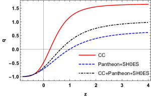
Figure 6: The deceleration parameter $(q)$ versus redshift $(z)$.

Figure (6) illustrates the behavior of the deceleration parameter for the corresponding value of the model parameters $m,n$, and $k$ specified by the $CC$ and $Pantheon+SH0ES$ data samples. It is observed that the transition value of redshift for the $CC$ dataset is found to be $z_{t}=0.235\pm 0.026$ and the present value of the deceleration parameter is $q_{0}=-0.474^{+0.111}_{-0.122}$. In the same way for $CC+Pantheon$ and $CC+Pantheon+SH0ES$ datasets, the transition values of redshift are obtained as $z_{t}=0.98^{+0.05}_{-0.049}$ and $z_{t}=0.649\pm 0.039$ and the present value of deceleration parameter $q_{0}=-0.711^{+0.042}_{-0.061}$ and $q_{0}=-0.662^{+0.066}_{-0.062}$ respectively. It is evident from the aforementioned values of $q_{0}$ for each dataset that, the $CC$ dataset is more compatible with the $\Lambda$CDM model.

The total or effective Equation-of-State $(\omega_{eff})$ as a function of Hubble parameter $H$ is given as

$$\omega_{eff}=-1-\frac{2}{3}\frac{\frac{d}{dt}H(z)}{H^{2}(z)},$$ (28)

where, $\frac{d}{dt}H(z)=-(1+z)H(z)\frac{d}{dz}H(z)$. The effective EoS as a whole determines a relation between the Hubble parameter and its derivative. The value of $\omega_{eff}$ of the model is obtained from equations (20) and (28) as

$$\omega_{eff}=-1+\frac{km(1+z)^{k}}{3n+3m(n-1)(1+z)^{k}}.$$ (29)

Figure 7: The EoS parameter $(\omega_{eff})$ versus redshift $(z)$ for constrained values of CC, Pantheon +SH0ES, and CC+Pantheon+SH0ES datasets.

The Equation-of-State parameter can indeed be useful in classifying the various phases, like the accelerated and decelerated expansion of the universe. According to the various phases, a stiff fluid is represented at $\omega=1$, the radiation-dominated phase is shown by $\omega=1/3$, and the matter-dominated phase is shown by $\omega=0$. Fig. (7) displays the evolution trajectory of the effective EoS parameter $\omega_{eff}$. The quintessence era $(-1<\omega<-1/3)$, the phantom era $(\omega<-1)$, and the cosmological constant $(\omega=-1)$ are the three conceivable states for the expanding universe. From Fig. (7) it is observed that for low redshift the value of the effective EoS parameter fluctuates between $-0.5$ to $-1$ i.e., quintessence dark energy, indicating an acceleration phase which is due to negative effective pressure of the universe explaining the presence of DE. The present value of $\omega_{eff}$, which corresponds to the constrained values of the model parameters, is obtained by fitting the model with the observational data as $\omega_{0}=-0.649^{+0.074}_{-0.081}$, $\omega_{0}=-0.807^{+0.028}_{-0.041}$, and $\omega_{0}=-0.744^{+0.043}_{-0.042}$. It is observed that the present value of $\omega_{eff}$ for the $Pantheon+SH0ES$ sample exhibits strong agreement with the $\Lambda$CDM model.

We attempt to examine additional parameters in $f(T)$ gravity. Expanding the scale factor in the Taylor series concerning cosmic time [36] indicates a relationship between distance and redshift. The higher-order derivatives of the deceleration parameter, which are referred to as jerk ($j$), snap ($s$), and lerk ($l$) parameters, appear in the Taylor series expansion. These parameters enable us to view the past and future status of the universe.

$$j=(1+z)\frac{dq}{dz}+q(1+2q),$$ (30)

$$s=-(1+z)\frac{dj}{dz}-q(2+3q),$$ (31)

$$l=(1+z)\frac{ds}{dz}-s(3+4q).$$ (32)

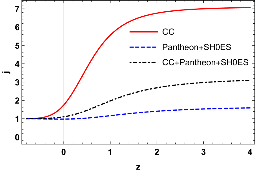
(a)

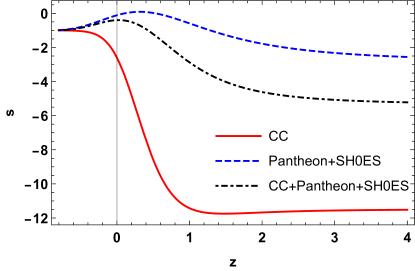
(b)

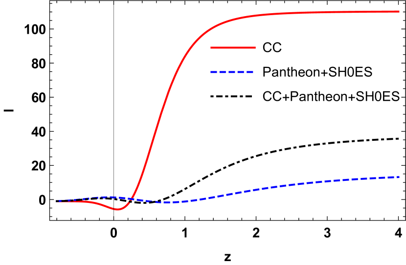
(c)

Figure 8: The jerk $(j)$, snap $(s)$, and lerk ($l$) parameter versus redshift $(z)$ for constrained values of CC, Pantheon +SH0ES, and CC+Pantheon+SH0ES datasets.

From Figs. (8(a)) and (8(c)) the jerk and lerk parameters are observed to have positively decreasing behavior (w.r.t. cosmic time $t$). The dynamics of the universe are controlled by the sign of the jerk parameter, a positive value denotes the existence of a transition phase during which the universe adapts its expansion. It is interesting to note that for given datasets the jerk parameter fails to attain unity at $z=0$, i.e., $j_{0}=1.741^{+0.368}_{-0.331},j_{0}=0.978^{+0.042}_{-0.049}$, and $j_{0}=1.102^{+0.121}_{-0.087}$ for $CC,Pantheon+SH0ES$, and $CC+Pantheon+SH0ES$ datasets, respectively, but it is observed that $CC+Pantheon+SH0ES$ datasets show the minimum error of $0.01$ as compared to others, so at present interval the model is more compatible with standard $\Lambda$CDM model for $CC+Pantheon+SH0ES$ dataset, and exhibit for every dataset in the future. To distinguish between the behavior of a cosmological constant and an evolving dark energy term, the snap parameter plays a crucial role. Fig. (8(b)) explains the accelerated expansion, which indicates negative behavior and approaches $-1$ for late time. It demonstrates how late-time acceleration can be noticed in a strictly geometrical way under certain modified gravity, like teleparallel gravity. At the current epoch, the values of the snap parameter are obtained as $s_{0}=-2.606^{+1.074}_{-1.170}$, $s_{0}=-0.110^{+1.071}_{-1.170}$, and $s_{0}=-0.399^{+.130}_{-0.260}$ for $CC,Pantheon+SH0ES$, and $CC+Pantheon+SH0ES$ datasets, respectively. A similar argument has been given by [37], which obtained the same results on these parameters.

V Om diagnostics

$Om$ is a tool for diagnosis that allows one to distinguish between $\Lambda$CDM with or without matter density and dynamical dark energy models. With positive slopes i.e., ($\omega<-1$) indicating a phantom-type model and negative slopes i.e., ($\omega>-1$) showing a quintessence-type model, its consistent behavior i.e., ($\omega=-1$) suggests dark energy is a cosmological constant ($\Lambda$CDM) [38]. The $Om(z)$ diagnostic for a spatially flat universe is defined as,

$$Om(z)=\frac{E^{2}(z)-1}{(1+z)^{3}-1},$$ (33)

where $E(z)=H(z)/H_{0}$.

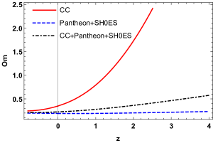
Figure 9: $Om$(z) diagnostic versus redshift ($z$) for constrained values of CC, Pantheon +SH0ES, and CC+Pantheon+SH0ES datasets.

Fig.(9) depicts the behavior of the dark energy model for different datasets. The value of $Om$(z) increases with an increase of $z$, which is observed for $CC$ and $CC+Pantheon+SH0ES$ datasets. It is observed that the model shows phantom-type behavior as the graph shows an upward trend, i.e., a positive slope ($\omega<-1$) for $CC$ and $CC+Pantheon+SH0ES$ datasets meanwhile, the model behaves like $\Lambda$CDM for $Pantheon+SH0ES$ dataset in the near future [39].

VI conclusion

In this article, we offer a comprehensive cosmological framework using the power law model of teleparallel gravity within the context of the FLRW universe. To obtain an exact solution of the field equations, we execute the parametrization of the effective EoS as per the [29]. Optimal results are obtained by pursuing the $\chi^{2}$ minimization technique to get the best-fit values of the model parameters $m,n$, and $k$, to do so, we utilize the dataset samples namely the $CC,Pantheon+SH0ES$ and joint analysis of $CC$ and $Pantheon+SH0ES$. Table (1) displays the constrained values parameters together with the $1-\sigma$ confidence error. Table (2) shows the best-fit values of cosmological parameters at the present interval of time. we have obtained the various cosmological parameters like the deceleration parameter, effective EoS parameter, $Om$ diagnostic, jerk, snap, and lerk parameters.

Various observational studies show different values of Hubble constant $H_{0}$. In modern cosmology, $H_{0}$-tension arises as a new problem, we can observe a checklist for different values of $H_{0}$ [40]. Due to this, we aspire to constrain the $H_{0}$ in the framework of the $f(T)$ gravity. For MCMC analysis, the constrained value of $H_{0}$ for the $CC$ sample is $H_{0}=68.89\pm 0.58$ $kms^{-1}Mpc^{-1}$ also for $Pantheon+SH0ES$ and $CC+Pantheon+SH0ES$ samples are $H_{0}=73.41^{+0.35}_{-0.29}$ $kms^{-1}Mpc^{-1}$ and $H_{0}=73.20^{+0.32}_{-0.24}$ $kms^{-1}Mpc^{-1}$ respectively. The behavior of the deceleration parameter as per Fig. (6) shows that at high redshift, the rate of accelerated expansion of the model increases for the $CC+Pantheon$ sample compared to others while the model transits into the de Sitter model for every dataset at low redshift. The present value deceleration parameter for the $CC$ sample is $q_{0}\approx-0.474$ representing similar cosmic acceleration as the $\Lambda$CDM model. The $CC$ shows an early and the $Pantheon+SH0ES$ sample shows a delayed transition to the $\Lambda$CDM model. The model shows $z_{t}\approx 0.649$ transition value for, $CC+Pantheon+SH0ES$ which holds a nearly similar value compared to $\Lambda$CDM. Overall, we can say that the model shows a transition from initial deceleration to late-time acceleration. Moving on, Fig. (7) explains the negative behavior of the effective EoS. At the current epoch, the model have $\omega_{0}=-0.649^{+0.074}_{-0.081}$, $\omega_{0}=-0.807^{+0.028}_{-0.041}$, and $\omega_{0}=-0.744^{+0.043}_{-0.042}$ for given observational dataset samples. Irrespective of each dataset, the model remains in the quintessence era at low redshift. i.e., does not cross the phantom-divide line ($\omega=-1$), which means in the future, the model will get closer to $-1$. In another way, the model leads to the Einstein-de Sitter model soon. Moreover, it has been discovered that the jerk parameter takes the value of $j_{0}=1.741^{+0.368}_{-0.331}$, which explains the super accelerated expansion for the $CC$ dataset meanwhile, the same model depicts the values $j_{0}=0.978^{+0.042}_{-0.049}$, and $j_{0}=1.102^{+0.121}_{-0.087}$, that explains the minor and more gradual shift in acceleration for $Pantheon+SH0ES$ and joint analysis of $CC$ and $Pantheon+SH0ES$ dataset respectively as per the Fig (8(a)). A noteworthy deviation is observed in the numerical value of the snap parameter $s(z)$ at high and low redshift for each data sample. Fig. (8(b)) predicts the lower value of $s(z)$ at high redshift. The present value of this parameter is $s_{0}=-2.606^{+1.074}_{-1.170}$ indicates the high negative deviation for the $CC$ meanwhile, $Pantheon+SH0ES$ and $CC+Pantheon+SH0ES$ dataset shows $s_{0}=-0.110^{+1.071}_{-1.170}$, and $s_{0}=-0.399^{+.130}_{-0.260}$ respectively, which indicates the low negative deviation from $\Lambda$CDM behavior. From Fig. (9) it is clear that the occurrence of $Om$(z) at late times is consistent with the breaking down of dark energy theory, and this model is consistent with the standard $\Lambda$CDM model for the $Pantheon+SH0ES$ dataset.

In conclusion, the power law model of the $f(T)$ gravity is consistent with the observational data and may serve as a potential description of dark energy. Additionally, from both statistical and cosmological perspectives, the derived $f(T)$ model is more compatible with the $\Lambda$CDM model for $Pantheon+SH0ES$ and $CC+Pantheon+SH0ES$ datasets compared to the $CC$.

Data Availability Statement

There are no new data associated with this article.

References

- [1] A. G. Riess, et al., Astron. J. 116, 1009 (1998).; S. Perlmutter, et al., Astrophys. J. 517, 565 (1999).
- [2] D. N. Spergel, et al., The Astrophy. J Supp. Series, 148, 175 (2003).; D. N. Spergel, et al., The Astrophy. J Supp. Series, 170, 377S (2007).
- [3] M. Tegmark, et al., Phys. Rev. D. 69, 103501 (2004).; D. J. Eisenstein, et al., Astrophys. J. 633, 560 (2005).
- [4] R. R. Caldwell, R. Dave and R. J. Steinhardt, Phys. Rev. Lett. 80, 1582 (1998).; R. R. Caldwell, Phys. Lett. B. 545, 23 (2002).; C. Armendariz-Picon, V. Mukhanov and P. J. Steinhardt, Phys. Rev. D. 63, 103510 (2001).; T. Padmanabhan, Phys. Rev. D. 66, 021301 (2002).; A. Sen, Phys. Scripta. T. 117, 70 (2005).; E. Elizadle, S. Nojiri and S. D. Odintsov, Phys. Rev. D. 70, 043539 (2004).; B. Feng, X. L. Wang and X. M. Zhang, Phys. Lett. B. 607, 35 (2005).
- [5] A. Kamenshchik, U. Moschella and V. Pasquier, Phys. Lett. B. 511, 265 (2001).
- [6] M. C. Bento, O. Bertolami and A. A. Sen, Phys. Rev. D. 66, 043507 (2002).
- [7] A. G. Cohen, D. B. Kaplan and A. E. Nelson, Phys. Rev. Lett. 82, 4971 (1999); M. Li, Phys. Lett. B. 603, 1 (2004).
- [8] H. Wei and R. G. Cai, Phys. Lett. B. 663, 1 (2008); H. Wei and R. G. Cai, Phys. Lett. B. 660, 113 (2008).
- [9] C. Gao, F. Wu, X. Chen and Y. G. Shen, Phys. Rev. D. 79, 043511 (2009).
- [10] S. M. Carroll, Living Rev. Rel. 4 (2001) 1; E. J. Copeland, M. Sami and S. Tsujikawa, Int. J. Mod. Phys. D. 15, 1753 (2006).
- [11] A. Paliathanasis, et al., Phys. Rev. D 94, 023525 (2016).
- [12] H.A. Buchdahl, Mon. Not. R. Astron. Soc., 150, 1 (1970).; S. Capozziello, V.F. Cardone, V. Salzano, Phys. Rev. D, 78, 063504 (2008).; M. Sharif and Z. Yousaf, Phys. Rev. D, 88, 024020 (2013).; G. Gadbail, S. Arora, and PK. Sahoo, et al., arXiv preprint arXiv:2402.04813, (2024).
- [13] S. Nojiri, S.D. Odintsov, Phys. Rev. D, 8, 74 (2006).; E. Elizalde, D. Saez-Gomez, Phys. Rev. D, 4, 80 (2009). A. de la Cruz-Dombriz, A. Dobado, Phys. Rev. D,8, 74 (2006).; S.A. Kadam, B. Mishra, and J.K. Said, Eur. Phys. J. C., 8, 82 (2022).
- [14] M. Z. Bhatti, Z. Yousaf, M. Yousaf, Phys. Dark Univ., 28, 100501 (2020).
- [15] E. Elizalde, M. Khurshudyan, Phys. Rev. D 98, 123525 (2018); E. Elizalde, M. Khurshudyan, Phys. Rev. D 99, 024051 (2019).
- [16] P. K. Sahoo, et al., Eur. Phys. J. C 78, 46 (2018).
- [17] T. Azizi, Int. J. Theor. Phys. 52, 3486 (2013).
- [18] S. Bahamonde, et al., Eur. Phys. J. C 77,1-8 (2017).
- [19] G. Gadbail, et al., Phys. Dark Uni. 37, 101074(2022).
- [20] S. Arora, et al., Phys. Dark Uni. 31, 100790(2021).
- [21] Y. Xu, G. Li, T. Harko and S.-D. Liang, Eur. Phys. J. C 79,1-19(2019).
- [22] G. R. Bengochea, R. Ferraro, Phys. Rev. D 79, 124019 (2009).
- [23] K. Bamba, et al., J. Cosmol. Astropart. Phys. 01, 021 (2011).; R. Myrzakulov, Eur. Phys. J. C 71, 1752 (2011).; G. Gadbail, S. Arora, P.K. Sahoo, Ann. Phys., 451, (2023).
- [24] K. Bamba, et al., Phys. Rev. D 94, 083513 (2016).
- [25] R. C. Nunes et al., J. Cosmol. Astropart. Phys. 1608, 011 (2016).; P. Wu, H. Yu, Phys. Lett. B 693, 415 (2010);P. Wu, H. Yu, Phys. Lett. B 692, 176 (2010).; B. Mirza, F. Oboudiat, J. Cosmol. Astropart. Phys. 11, 011 (2017).; L.K. Duchaniya, K. Gandhi, and B. Mishra, Phy. Dark Uni., 44, 101461 (2024).
- [26] R.C.Nunes, JCAP , 2018,052 (2018).
- [27] M. Blagojevic’ et al., Physical Rev. D. 6, 109 (2024).
- [28] R. Chen, Y.Y. Wang, Y.Z. Fan, L. Zu, Physical Rev. D. 2, 109 (2024).
- [29] A. Mukherjee, Mon. Not. R. Astron. Soc., 1, 460 (2016).
- [30] R. Aldrovandi and J.G. Pereira, Springer Sci., (2013).; G. R. Bengochea, Phys. Lett. B, 5 695, 405 (2011).; S. Bahamonde, K.F. Dialektopoulos, et al., Rep. Progr. Phys., 2, 86 (2023).
- [31] Y. F. Cai, et al., Rep. Progr. Phys. 10,79, 106901 (2016).
- [32] J.W. Maluf, Annalen Phys. 5, 525 (2013).
- [33] M.Hobson, et al., Camb. Uni. Press., (2010).
- [34] H. Singirikonda, S. Desai, Eur. Phys. J. C., 80, 694 (2020).
- [35] M. Kowalski, D. Rubin, et al., The Astrophys. J., 686, 749 (2008).; R. Amanullah, C. Lidman et al., The Astrophys. J., 716, 712 (2010).; N. Suzuki, D. Rubin, et al., The Astrophys. J., 746, 85 (2012).; M. Betoule, R. Kessler, et al., Astronomy & Astrophysics, 568, A22 (2014).; D. Scolnic, D. Jones, et al., The Astrophys. J., 859, 101 (2018).
- [36] S. Weinberg, Gravitation and Cosmology Principles and Applications of the General Theory of Relativity, Wiley (1972).
- [37] S. Mandal, et al., Phys. Dark Uni., 28, 100551 (2020).; S. Arora et al., Physica Scripta, 95, 095003 (2020).; R. Nagpal, J.K.Singh, et al., Annals of Phys., 405, 234-255 (2019).; R. Mishra, et al., Astrophy. Space Sci., 366, 47 (2021).
- [38] V. Sahni, A. Shafieloo, A. A. Starobinsky, Phys. Rev. D, 78, 103502 (2008).; C. Zunckel, C. Clarkson, Phys. Rev. Lett., 101, 181301 (2008).
- [39] P. Thakur, IJP, 3, 96 (2022).; A.Al. Mamon, V.C. Dubey, Bamba, Universe, 7, 10 (2021).; S. Arora, X. Meng, P.K. Sahoo, et al., Class. Quant. Grav., 20, 37, 205022 (2020).; A. Shafieloo, V. Sahni, A.A. Starobinsky, Phys. Rev. D. Part., 10, 80 (2009).
- [40] R. Verma, M. Kashav, et al., PTEP, 3, 2022 (2022).; J. Henning, J. Sayre, C. Reichardt, et al., Astrophy. J., 2, 97 (2018).; S. Aiola, E. Calabrese, L. Maurin, S. Naess, et al.,Astropart. Phys., 12,47 (2020).