BCDNet: A Convolutional Neural Network For Breast Cancer Detection

Abstract

Previous research has established that breast cancer is a prevalent cancer type, with Invasive Ductal Carcinoma (IDC) being the most common subtype. The incidence of this dangerous cancer continues to rise, making accurate and rapid diagnosis, particularly in the early stages, critically important. While modern Computer-Aided Diagnosis (CAD) systems can address most cases, medical professionals still face challenges in using them in the field without powerful computing resources. In this paper, we propose a novel CNN model called BCDNet, which effectively detects IDC in histopathological images with an accuracy of up to 89.5% and reduces training time effectively. The code is available at https://github.com/YujiaLin-523/BCDNet

I Introduction

In 2020, there were 2.26 million new breast cancer cases and 0.684 million deaths reported globally, making breast cancer the most frequently diagnosed cancer and the fourth leading cause of cancer-related deaths among 36 cancer types [1]. The incidence of breast cancer has been rising by 0.5% annually from 2010 to 2019 [2]. Invasive Ductal Carcinoma (IDC) is the predominant subtype of breast cancer, accounting for 80% of all cases [3].

Despite the availability of various diagnostic methods such as mammography, digital breast tomosynthesis, breast ultrasound, and magnetic resonance imaging, accurately and rapidly diagnosing breast cancer and IDC remains a significant challenge for radiologists and other medical staff due to the increasing number of patients and the complexity of the diagnostic process. To assist pathologists, Computer-Aided Diagnosis (CAD) systems have been developed as complementary tools to conventional diagnostic methods [4, 5]. These systems analyze medical images or other data and provide diagnostic results to pathologists, specifically aiding in the diagnosis of IDC by saving time while maintaining accuracy. The continuous advancements in Deep Learning, especially in Computer Vision, contributes a lot to the improvement of CAD. In Medical Image Processing, CNN-based methods are widely used for breast cancer detection due to CNN’ s ability to learn features automatically rather than relying on hand-crafted features. However, current CNN models are often challenging to train due to their relatively large number of parameters and the limited computing resources in some medical institutions. This limitation hampers the ability to quickly adapt to changes in datasets, such as the emergence of a new type of cancer. To address this, we developed BCDNet that is both efficient and easy to train, enabling deployment on edge devices and rapid modification for new datasets. Our main contributions can be concluded as follows:

• We propose a novel architecture BCDNet, which is efficient and easy to train.

• We prove the superiority of BCDNet by comparing it with ResNet 50 and ViT-B-16.

II Related Work

II-A Conventional Methods

To diagnose breast cancer, four conventional methods are commonly employed: Mammography, Digital Breast Tomosynthesis (DBT), Breast Ultrasound, and Magnetic Resonance Imaging (MRI) [1, 3, 6, 7, 8, 9]. Mammography, an initial method for early-stage breast cancer detection using X-ray to obtain 2D images, is divided into screening mammography and Digital Mammography (DM). As imaging technology rapidly advances, new diagnostic opportunities emerge. DBT, more mature than DM, offers a novel way of observing breast cancer images by capturing 2D slices and synthesizing them into 3D images. This reduces tissue overlap and enhances diagnostic accuracy. Automatic Breast Ultrasound (ABUS) enables radiologists to diagnose breast cancer with greater accuracy through improved imaging frequency. Additionally, MRI diagnoses breast cancer using magnetic fields and radio waves to capture detailed images.

III Method

Figure 1: The architecture of BCDNet. We combine Convolutional layers, Pooling layers and ReLU with BatchNorm to build this model.

The architecture of BCDNet is shown in Fig. 1. The model consists of a series of convolutional layers, pooling layers, activation layers, fully-connected layers, Batch Normalization layers and Dropout layers. This structured combination of layers is designed to efficiently and accurately detect IDC in histopathological images. In the following sections, we will delve into the specific configurations and functionalities of each layer type within BCDNet.

III-A Convolutional Layer

Convolutional Neural Networks (CNNs) employ a mathematical operation called convolution for the purpose of feature extraction [10, 11, 12]. This operation, a fundamental aspect of CNNs, is simply depicted in the following equation:

$$F=I*K$$ (1)

where $F$ represents the feature map, $I$ is the input, and $K$ is the kernel. The kernel, a matrix of weights, is paramount in extracting significant features from the input, thereby enabling the network to learn and identify various patterns. The kernel’s weights are optimized using backpropagation to minimize the loss function. This convolution process can also be illustrated in detailed by

$$s(t)=(x*w)(t)=\sum_{a=-\infty}^{+\infty}x(a)w(t-a)$$ (2)

Feature maps in CNN are generated by convolving a kernel with the input data. CNNs employ parameter sharing, where the same kernel weights are reused across different input regions, significantly reducing the total number of parameters needed. This approach efficiently captures complex patterns and features across various images while maintaining a simpler model structure.

III-B Pooling Layer

Pooling is an essential down-sampling method used in CNN to enhance invariance and combine semantically similar features, thus ensuring robust feature extraction [10]. The primary goal of pooling is to reduce the spatial dimensions of a feature map, thereby decreasing the amount of data while preserving crucial features for the learning process. Max pooling, a common pooling operation, selects the largest value within a designated window or kernel area, effectively reducing the dimensionality of the feature map and making the representation less sensitive to minor shifts or alterations in the input.

In mathematical terms, consider a feature map $F$ of dimensions $i\times j$, and a pooling window (or kernel) $P$ of size $k\times k$. Max pooling can be expressed as:

$$M(i,j)=\max_{0<p,q\leq k}F_{i+p,j+q}$$ (3)

where $M$ is the down-sampled feature map, and $M_{(i,j)}$ is the maximum value within the $k\times k$ window centered at $(i,j)$ in the original feature map. Max pooling, a fundamental technique in convolutional neural networks (CNNs), involves sliding a pooling window over the feature map and selecting the maximum value within each region. This process effectively reduces the dimensionality of the feature map while retaining its most salient features, thereby enhancing the network’s efficiency and ability to extract invariant features. In summary, max pooling is crucial in CNNs for down-sampling, enhancing invariance, and pinpointing the most prominent features within the input data.

III-C Activation Layer

The Rectified Linear Unit (ReLU), is a widely utilized activation function in neural networks [13]. The function is defined as the following equation and can be seen in, equates values less than zero to zero, and values greater than or equal to zero to passed in value.

$$f(x)=max(0,x)=\begin{cases}0,x\leq 0\\ x,x>0\end{cases}$$ (4)

ReLU introduces non-linearity into neural networks without compromising computational efficiency, avoiding the vanishing gradient problem seen in sigmoid and tanh functions. This property allows neural networks to learn complex patterns more effectively. Additionally, ReLU prevents gradient saturation, facilitating faster and more efficient training. ReLU is critical in modern neural networks for its role in enhancing non-linearity, improving computational speed, and aiding in model convergence.

III-D Fully-Connected Layer

The Fully-Connected (FC) layer can be viewed as performing a mapping of all the features in a given feature space [10, 11, 12]. Its task is to transform these features through a combination of linear operations followed by non-linear activation functions, enabling complex decision-making processes. In CNN, the FC layer processes the features extracted by the convolutional and pooling layers and maps them to the final decision output. This can be expressed mathematically as:

$$y=f(Wx+b)$$ (5)

where x represents the input features, $W$ is the weight matrix, $b$ is the bias term, $f$ is the activation function ReLU in our work, and $y$ is the output. In the upper representation, $Wx$ denotes a linear transformation that maps the input vector $x$ into a new space. The weight matrix $W$ in an FC layer assigns a unique set of weights to each row, combining input features to compute each output neuron’s value. The bias b adjusts this mapping, increasing the model’s flexibility. This mapping transforms processed features into new representations, suitable for final decision-making tasks. This integration and transformation of features in the FC layer are crucial for supporting classification, regression, and other decision-making tasks in neural networks.

III-E Batch Normalization Layer

Batch Normalization enhances model performance and stability by normalizing layer inputs during training, mitigating issues like exploding gradients. Additionally, it can accelerate convergence since it transforms inputs into a certain distribution. In CNN, Batch Normalization plays a crucial role by normalizing the outputs of convolutional layers, ensuring that each layer receives inputs with a consistent scale. This process helps stabilize and speed up the training of deep CNNs. By reducing internal covariate shift, Batch Normalization allows for higher learning rates, thereby improving training efficiency and model performance [14]. Given input x, this process is:

$$y_{i}=\frac{\gamma(x_{i}-\mu)}{\sigma}+\beta$$ (6)

where $y_{i}$ is the normalized output, $\gamma$ and $\beta$ are learnable parameters, $\mu$ and $\sigma$ are the mean and standard deviation of the small batch of input, respectively.

III-F Dropout

Dropout is a regularization technique used to prevent overfitting in neural networks [15]. By randomly setting a fraction p of the neurons’ activations to zero during the training, the network is encouraged to learn more robust features, thereby improving its generalization capabilities. The dropout process can be expressed as:

$$h_{i}=\begin{cases}0,\text{with probability }p\\ \frac{x_{i}}{1-p},\text{otherwise}\end{cases}$$ (7)

Here, $p$ is the dropout rate, and the scaling factor $1/(1-p)$ ensures that the expected sum of the activations remains consistent during both training and inference.

IV Experiments

To evaluate BCDNet’s performance, we conducted a comprehensive experiment between BCDNet, ResNet50 and ViT-B-16, which are renowned for their robust performance in image classification tasks. ResNet50, a deep residual network, is celebrated for its pioneering use of residual learning to solve vanishing gradient problems [16], while ViT-B-16, a Vision Transformer, represents a shift towards transformer architectures in computer vision, demonstrating strong performance by leveraging self-attention mechanisms [17]. Training was conducted on a server with 2 NVIDIA RTX 4090 GPUs, leveraging a cross-entropy loss function and the Adam optimizer. The learning rate was initially set to 0.005, with a StepLR scheduler to facilitate convergence. Our study is based on two open-source IDC image datasets, and we assess models on accuracy, training time, and memory consumption. The results are summarized in Fig 2 and Table I.

Figure 2: The accuracy and training time of BCDNet, ResNet 50 and ViT-B-16 on IDC regular dataset.

Figure 3: The accuracy and training time of BCDNet, ResNet 50 and ViT-B-16 on BreaKHis v1 dataset.

IV-A Dataset

In this study, we firstly utilized an Invasive Ductal Carcinoma (IDC) image dataset from kaggle, which is termed as IDC regular by us in this paper. IDC regular dataset comprises histopathological scans of breast cancer tissues, annotated to indicate the presence or absence of IDC. Meanwhile, we also use BreaKHis v1 dataset, which is composed of multiple types of breast cancer histopathology images obtained under various imaging conditions. The two datasets are divided into training, validation and testing sets by a proportion of 7:2:1 respectively to enable the evaluation of our proposed model, BCDNet, against established benchmarks.

IV-B Data Augmentation

Data augmentation is a strategy designed to expand the size of a dataset, enhancing both the model’s performance and robustness to overfitting [11]. It involves generating new training samples by applying various transformations to the original data.

In our study, we first applied Normalization to every image to accelerate the training. Then, we used random horizontal and vertical flipping and random rotation to increase the diversity of the training set. Finally, all the images were resized to $224\times 224$ pixels to ensure consistency in the input dimensions.

IV-C Evalution Metrics

We evaluated the models based on accuracy, training time, and GPU memory consumption. Training time and memory usage were monitored to highlight the efficiency of each model. Accuracy was assessed on an independent test set to ensure fair comparison.

IV-D Results

Based on Fig 2, 3, 4, 5 and Table I, we can summarize that though BCDNet has a slightly lower accuracy than ResNet 50, it is more efficient in terms of training time and memory consumption even though we used pretrained models of ResNet and ViT in our experiments. BCDNet is more suitable for deployment on edge devices and can be quickly modified for new datasets. Moreover, the convergence speed of BCDNet is also higher. Its loss and accuracy both become stable quite early.

TABLE I: The Memory Consumption of BCDNet, ResNet 50 and ViT-B-16.

Model	Datasets
Types	IDC regular	BreaKHis v1
BCDNet	4.8 GB	4.5 GB
ResNet 50	16.7 GB	16.6 GB
ViT-B-16	20.8 GB	20.8 GB

Figure 4: The accuracy and loss curves of the three models on IDC regular dataset. From up to down, the three models are BCDNet, ResNet 50, and ViT-B-16.

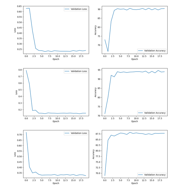
Figure 5: The accuracy and loss curves of the three models on BreaKHis v1 dataset. From up to down, the three models are BCDNet, ResNet 50, and ViT-B-16.

V Conclusion

In this paper, BCDNet has shown its advantages that it consumes much less training time and memory consumption while loses a little accuracy, which means it is suitable for the medical system in the impoverished areas or in the wild.

Although we have leveraged a novel architecture to enhance the speed of the model, the accuracy of BCDNet is still not high enough. In the future, the model can be continously improved by using Layer Freezing, which is widely used to minimize the number of parameters. Additionally, Post-Training Quantization (PTQ) can be probably applied to accelerate the whole process when increasing the depth of the model.

References

- [1] T. Kwong and S. Mazaheri, “A survey on deep learning approaches for breast cancer diagnosis,” Feb. 2022, arXiv:2109.08853 [cs, eess]. [Online]. Available: http://arxiv.org/abs/2109.08853
- [2] “Breast Cancer Diagnosis and Screening | AAFP.” [Online]. Available: https://www.aafp.org/pubs/afp/issues/2000/0801/p596.html
- [3] L. Wang, “Early Diagnosis of Breast Cancer,” Sensors, vol. 17, no. 7, p. 1572, Jul. 2017, number: 7 Publisher: Multidisciplinary Digital Publishing Institute. [Online]. Available: https://www.mdpi.com/1424-8220/17/7/1572
- [4] R. M. Rangayyan, F. J. Ayres, and J. E. Leo Desautels, “A review of computer-aided diagnosis of breast cancer: Toward the detection of subtle signs,” Journal of the Franklin Institute, vol. 344, no. 3, pp. 312–348, May 2007. [Online]. Available: https://www.sciencedirect.com/science/article/pii/S001600320600127X
- [5] J. Tang, R. M. Rangayyan, J. Xu, I. E. Naqa, and Y. Yang, “Computer-Aided Detection and Diagnosis of Breast Cancer With Mammography: Recent Advances,” IEEE Transactions on Information Technology in Biomedicine, vol. 13, no. 2, pp. 236–251, Mar. 2009, conference Name: IEEE Transactions on Information Technology in Biomedicine. [Online]. Available: https://ieeexplore.ieee.org/abstract/document/4757273
- [6] E. S. McDonald, A. S. Clark, J. Tchou, P. Zhang, and G. M. Freedman, “Clinical Diagnosis and Management of Breast Cancer,” Journal of Nuclear Medicine, vol. 57, no. Supplement 1, pp. 9S–16S, Feb. 2016. [Online]. Available: http://jnm.snmjournals.org/lookup/doi/10.2967/jnumed.115.157834
- [7] “Sensors | Free Full-Text | Early Diagnosis of Breast Cancer.” [Online]. Available: https://www.mdpi.com/1424-8220/17/7/1572
- [8] “Journal of Cellular Physiology | Cell Biology Journal | Wiley Online Library.” [Online]. Available: https://onlinelibrary.wiley.com/doi/abs/10.1002/jcp.26379
- [9] “Breast Cancer Statistics, 2022 - Giaquinto - 2022 - CA: A Cancer Journal for Clinicians - Wiley Online Library.” [Online]. Available: https://acsjournals.onlinelibrary.wiley.com/doi/full/10.3322/caac.21754
- [10] Z. Li, F. Liu, W. Yang, S. Peng, and J. Zhou, “A Survey of Convolutional Neural Networks: Analysis, Applications, and Prospects,” IEEE Transactions on Neural Networks and Learning Systems, vol. 33, no. 12, pp. 6999–7019, Dec. 2022, conference Name: IEEE Transactions on Neural Networks and Learning Systems. [Online]. Available: https://ieeexplore.ieee.org/abstract/document/9451544
- [11] K. O’Shea and R. Nash, “An Introduction to Convolutional Neural Networks,” Dec. 2015, arXiv:1511.08458 [cs]. [Online]. Available: http://arxiv.org/abs/1511.08458
- [12] S. Albawi, T. A. Mohammed, and S. Al-Zawi, “Understanding of a convolutional neural network,” in 2017 International Conference on Engineering and Technology (ICET), Aug. 2017, pp. 1–6. [Online]. Available: https://ieeexplore.ieee.org/abstract/document/8308186
- [13] X. Glorot, A. Bordes, and Y. Bengio, “Deep Sparse Rectifier Neural Networks,” in Proceedings of the Fourteenth International Conference on Artificial Intelligence and Statistics. JMLR Workshop and Conference Proceedings, Jun. 2011, pp. 315–323, iSSN: 1938-7228. [Online]. Available: https://proceedings.mlr.press/v15/glorot11a.html
- [14] S. Ioffe and C. Szegedy, “Batch Normalization: Accelerating Deep Network Training by Reducing Internal Covariate Shift,” in Proceedings of the 32nd International Conference on Machine Learning. PMLR, Jun. 2015, pp. 448–456, iSSN: 1938-7228. [Online]. Available: https://proceedings.mlr.press/v37/ioffe15.html
- [15] Y. Gal and Z. Ghahramani, “Dropout as a Bayesian Approximation: Representing Model Uncertainty in Deep Learning,” in Proceedings of The 33rd International Conference on Machine Learning. PMLR, Jun. 2016, pp. 1050–1059, iSSN: 1938-7228. [Online]. Available: https://proceedings.mlr.press/v48/gal16.html
- [16] K. He, X. Zhang, S. Ren, and J. Sun, “Deep Residual Learning for Image Recognition,” 2016, pp. 770–778. [Online]. Available: https://openaccess.thecvf.com/content_cvpr_2016/html/He_Deep_Residual_Learning_CVPR_2016_paper.html
- [17] K. Han, Y. Wang, H. Chen, X. Chen, J. Guo, Z. Liu, Y. Tang, A. Xiao, C. Xu, Y. Xu, Z. Yang, Y. Zhang, and D. Tao, “A Survey on Vision Transformer,” IEEE Transactions on Pattern Analysis and Machine Intelligence, vol. 45, no. 1, pp. 87–110, Jan. 2023, conference Name: IEEE Transactions on Pattern Analysis and Machine Intelligence. [Online]. Available: https://ieeexplore.ieee.org/abstract/document/9716741