Circuit QED Emission Spectra in the Ultrastrong Coupling Regime:
How They Differ from Cavity QED

Abstract

Cavity quantum electrodynamics (QED) studies the interaction between resonator-confined radiation and natural atoms or other formally equivalent quantum excitations, under conditions where the quantum nature of photons is relevant. Phenomena studied in cavity QED can also be explored using superconducting artificial atoms and microwave photons in superconducting resonators. These circuit QED systems offer the possibility to reach the ultrastrong coupling regime with individual artificial atoms, unlike their natural counterparts. In this regime, the light-matter coupling rate reaches a considerable fraction of the bare resonance frequencies in the system. Here, we provide a careful analysis of the emission spectra in circuit QED systems consisting of a flux qubit interacting with an LC resonator. Despite these systems can be described by the quantum Rabi model, as the corresponding cavity QED ones, we find distinctive features, depending on how the system is coupled with the output port, which become evident in the ultrastrong coupling regime.

I Introduction

Superconducting quantum circuits (SQCs) based on Josephson junctions can behave like artificial atoms. They have made possible to implement atomic-physics and quantum-optics experiments on a chip [1]. In contrast to natural atoms, superconducting artificial atoms can be designed, fabricated, and controlled for various research purposes [2, 3, 4]. Furthermore, the interaction between artificial atoms and electromagnetic fields can be controlled and engineered with more freedom [5, 6, 7].

Superconducting artificial atoms have been used to demonstrate phenomena that cannot be realized or observed in quantum optics experiments with natural atoms. For instance, single- and two-photon processes can coexist in SQCs [8, 9], and the coupling between them and microwave fields can become ultrastrong. The ultrastrong coupling (USC) regime was observed for the first time in circuit QED systems in 2010 [10, 11], where normalized coupling strengths $\eta=0.10-0.12$ were achieved. Within this platform, it is possible to explore the light-matter USC regime with a single two-level system (qubit), instead of considering many atoms or collective excitations [12, 13].

The dimensionless parameter $\eta=g/\omega_{0}$, i.e., the cavity-emitter coupling rate divided by the qubit transition frequency (or the resonance frequency of a cavity mode), is used to quantify this coupling regime. Typically, USC effects are expected when $\eta\gtrsim 0.1$. At this value the rotating wave approximation (RWA) used in the weak and strong regimes starts to fail [14, 11, 12] and novel physical processes can be unlocked.

Recently, experiments in USC circuit QED are demonstrating a number of intriguing effects predicted theoretically [15, 16]. For a correct and complete comparison between theory and data, accurate models for circuit QED systems are highly desired.

Here, we present a theoretical framework for the calculation of emission spectra in circuit QED systems, working properly for arbitrary light-matter interaction strengths, ranging from the weak to the deep strong coupling (DSC) regime (coupling rates larger than the bare resonance frequencies). We study incoherent emission spectra for different coupling strengths and flux offsets under thermal-like excitation of the artificial superconducting atom. Specifically, we examine a flux qubit-LC oscillator system where each of the two subsystems is coupled to the environment. As in usual experimental settings, we consider output photons escaping the resonator through its coupling with a coplanar open transmission line (TL). We examine two cases: (i) resonator-TL interaction through mutual inductance; (ii) capacitive resonator-TL coupling. We show that the kind of resonator-TL coupling has to be included in the model in order to provide a quantitative description of the emission process, when the system enters the USC regime. We find that the nature of such coupling can affect spectra. We also compare the numerically calculated spectra with the corresponding cavity QED ones.

II Theoretical Framework

In this section, we consider a circuit QED system composed by a flux qubit galvanically coupled to an LC resonator [13, 17, 18]. We also study the coupling of this system, through a mutual inductance $M$, to an infinite TL [see Fig. 1(a)], then the capacitive coupling of the qubit-LC circuit with a semi-infinite TL [see Fig. 1(b)]. The full canonical quantization procedure is described in Appendix A.

II.1 Generalized Quantum Rabi Model

A key feature of the flux qubit is the strong anharmonicity of its energy spectrum, hence permitting a safe two-level approximation even in the presence of very high light-matter coupling strengths [18]. Thus, the Hamiltonian of the flux qubit can be easily written in the first two energy states basis ($\{\ket{g},\ket{e}\}$) as $\hat{\mathcal{H}}_{q}=\omega_{0}\,\hat{\sigma}_{z}/2$ (henceforth $\hbar=1$), where $\omega_{0}=\sqrt{\Delta^{2}+\epsilon^{2}}$. Here, $\Delta$ is the tunnel splitting and $\epsilon=2I_{p}(\Phi_{ext}-\,\Phi_{0}/2)$ the energy bias between the supercurrents flowing in opposite directions ($\{\ket{L},\ket{R}\}$), where $I_{p}$ is the critical current of the qubit, $\Phi_{\rm ext}$ is the external magnetic flux applied to the superconducting loop, and $\Phi_{0}$ is the flux quantum [3, 17, 18, 19, 20, 21]. The node flux $\hat{\Phi}_{q}$ across the qubit and the coupler $L_{C}$ can also be projected on the $\{\ket{g},\ket{e}\}$ basis giving as result $\hat{\Phi}_{q}\simeq I_{p}L_{C}\,\hat{\tilde{\sigma}}_{x}$, where $\cos{\theta}=\epsilon/\omega_{0}$, $\sin{\theta}=\Delta/\omega_{0}$, and $\hat{\tilde{\sigma}}_{x}=(\cos{\theta}\,\hat{\sigma}_{z}-\sin{\theta}\,\hat{\sigma}_{x})$; note that potential non-linear terms have been disregarded.

Regarding Fig. 1(a), the total Hamiltonian (including the input-output transmission line) can be written as

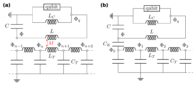
Figure 1: (a) Circuit diagram of a flux qubit galvanically coupled to the LC resonator. The infinite transmission line interacts with the inductance $L$ of the LC resonator through the mutual inductance $M$. The dynamical variables are indicated by the nodes. (b) Now, the semi-infinite transmission line is connected to the system through the capacitor $C_{K}$.

$$\hat{\mathcal{H}}_{M}=\hat{\mathcal{H}}_{0}+\hat{\mathcal{H}}_{\rm tl}+\hat{\mathcal{V}}_{M}\,.$$ (1)

In Eq. (1), $\mathcal{\hat{H}}_{0}$ describes the qubit-LC and their galvanic interaction:

$$\mathcal{\hat{H}}_{0}=\dfrac{\omega_{0}}{2}\hat{\sigma}_{z}+\omega_{r}\hat{a}^{\dagger}\,\hat{a}+\omega_{r}\,\eta(\hat{a}^{\dagger}+\hat{a})\hat{\tilde{\sigma}}_{x}\,,$$ (2)

where $\eta=L_{C}I_{p}\,I_{\rm zpf}/\omega_{r}$ is the resonator-qubit coupling normalized with respect to the resonance frequency $\omega_{r}\simeq 1/\sqrt{(L_{C}+L)C}$ of the LC oscillator, current $I_{\rm zpf}$ and flux $\Phi_{\rm zpf}$ zero-point fluctuations are related so that $I_{\rm zpf}=\Phi_{\rm zpf}/L$. Moreover, $\hat{\mathcal{H}}_{tl}=\int_{0}^{+\infty}d\omega\,\omega\,b^{\dagger}_{\omega}b_{\omega}$, where $b_{\omega}(b^{\dagger}_{\omega})$ are the bosonic creation (annihilation) operators for the continuum frequency modes of the TL; with $\commutator{b_{\omega}}{b^{\dagger}_{\omega^{\prime}}}=\delta(\omega-\omega^{\prime})$.

The mutual interaction term can be written as

$$\hat{\mathcal{V}}_{M}=i\,\frac{1}{\Phi_{\rm zpf}}\,\hat{\Phi}_{L}\int_{0}^{+\infty}d\omega\,\alpha\Phi_{\rm zpf}\,\frac{\Lambda}{v_{0}}\,\sqrt{\omega}\,[\hat{b}_{\omega}-\hat{b}^{\dagger}_{\omega}]\,,$$ (3)

where $\hat{\Phi}_{L}=\Phi_{\rm zpf}(\hat{a}+\hat{a}^{\dagger}-2\eta\,\hat{\tilde{\sigma}}_{x})$ and $\Lambda=\sqrt{{Z_{0}}/{4\pi}}$, with $Z_{0}$ being the TL impedance, $\alpha=M/L\,l_{T}$, and $v_{0}=1/\sqrt{l_{T}\,c_{T}}$ the velocity of the light in the TL; $l_{T}=L_{T}/\Delta x$ and $c_{T}=C_{T}/\Delta x$ are the inductance and the capacitance at each site of the TL per unit of length, $\Delta x$ being the distance between two sites.

It is worth stressing that whatever variation of the applied flux, which is proportional to $\epsilon$, would modify the resonance frequency of the LC circuit $\omega_{r}$, $I_{\rm zpf}$, and, as a consequence, the normalized coupling due to the presence of the coupler $L_{C}$. However, in this theoretical framework, $\omega_{r}$ and $I_{\rm zpf}$ are assumed to be independent from $\epsilon$. A thorough analysis about this aspect can be found in Refs. [17, 16].

Figure 1(b) displays the flux qubit-LC-oscillator system capacitively coupled to the TL. We will show that the different coupling mechanisms in Fig. 1(a) and (b) can influence the observed spectra, especially when the coupling between the flux qubit and the LC oscillator reaches the USC or DSC regime. In this case the total Hamiltonian is

$$\hat{\mathcal{H}}_{C}=\hat{\mathcal{H}}_{0}+\hat{\mathcal{H}}_{\rm tl}+\hat{\mathcal{V}}_{C}\,,$$ (4)

where the interaction with the TL reads as

$$\hat{\mathcal{V}}_{C}=\;i(\hat{a}^{\dagger}-\hat{a})\,\int_{0}^{+\infty}d\omega\,g(\omega)\,i(\hat{b}^{\dagger}_{\omega}-\hat{b}_{\omega})\,,$$ (5)

being $g(\omega)=\sqrt{\kappa\,\omega/\omega_{r}}$ , with ${\sqrt{\kappa}=C_{K}\,\omega_{r}/\sqrt{2\pi\,v_{0}c_{T}C}}$. We observe that the system operator $\hat{X}_{C}=i(\hat{a}^{\dagger}-\hat{a})$, appearing in the system-TL interaction Hamiltonian Eq. (5), differs from that in the case of inductive coupling: $\hat{X}_{M}=\hat{a}+\hat{a}^{\dagger}-2\eta\,\hat{\tilde{\sigma}}_{x}$.

II.2 Master Equation and Emission Spectra

In the following we will diagonalize numerically the closed system Hamiltonian $\mathcal{\hat{H}}_{0}$ and will treat the interaction of the system with the external reservoirs, including the input-output transmission line, within a master equation approach suitable for light-matter systems in the USC regime.

Both Eq. (1) and Eq. (4) lead to generalized master equations (GMEs), as discussed in Ref. [22]:

$$\dot{\hat{\rho}}=-i\commutator{\mathcal{\hat{H}}_{0}}{\hat{\rho}}+\mathcal{L}_{g}\,\hat{\rho}\,.$$ (6)

The Liouvillian superoperator involves the operators that are responsible for the interaction of the system with the baths (the complete equation is presented in Appendix B). The TL schematically displayed in Fig. 1 is one of the system baths. Additional bath-channels can, for example, describe qubit spontaneous emission losses and internal losses of the resonator. We also observe that the two different schemes in Fig. 1(a) and (b) give rise to different terms in the Liouvillian superoperator (see Appendix B). Regarding the qubit, we assume that the interaction with the relative reservoir occurs through the operator $\hat{\tilde{\sigma}}_{x}$ for both cases (the same operator in the qubit-LC interaction term).

Also, the damping rates of the system are reported in Appendix B.

In Appendix C, we present the derivation of the input-output voltage relations for both cases. In particular, we find that for the inductive coupling

$$\hat{V}^{\pm}_{M_{\rm out}}(x,t)=\hat{V}^{\pm}_{\rm in}(x,t)-\,\frac{M}{2L}\,\dot{\hat{\Phi}}^{\pm}_{L}(x,t)\,,$$ (7)

and for the capacitive coupling

$$\hat{V}^{\pm}_{C_{\rm out}}(t-x/v_{0})=\hat{V}^{\pm}_{in}(t+x/v_{0})+Z_{0}\frac{C_{K}}{C}\dot{\hat{Q}}^{\pm}(t-x/v_{0})\,.$$ (8)

Here, the $\pm$ label indicates positive $(+)$ and negative $(-)$ frequency operators. In the following, we will present emission spectra under incoherent (thermal-like) qubit excitation, in the absence of input drive $\left\langle{\hat{V}^{\pm}_{in}}\right\rangle\approx 0$. As a consequence, for the configuration in Fig. 1(a), the voltage measured from the opened port is determined by the following system operator [see Eq. (7)]

$$\dot{\hat{\Phi}}_{L}\propto\dot{\hat{X}}_{M}=\bigg{[}i\,(\hat{a}^{\dagger}-\hat{a})-2\eta\,\frac{\omega_{0}}{\omega_{r}}\sin{\theta}\,\hat{\sigma}_{y}\bigg{]}\,,$$ (9)

concerning the configuration displayed in Fig. 1(b), the output voltage is determined by

$$\dot{\hat{Q}}\propto\dot{\hat{X}}_{C}=-(\hat{a}^{\dagger}+\hat{a}+2\,\eta\,\hat{\tilde{\sigma}}_{x})\,.$$ (10)

Once the density matrix at the steady state $\hat{\rho}_{ss}$ is numerically derived from Eq. (6), applying the quantum regression theorem [23, 24], the power spectrum can be expressed as

$$S_{M(C)}(\omega)\propto\real\int_{0}^{+\infty}\!\!\!\!d\tau\,e^{-i\omega\tau}\left\langle{\dot{\hat{X}}_{M(C)}^{(-)}(t+\tau)\dot{{\hat{X}}}_{M(C)}^{(+)}(t)}\right\rangle_{ss},$$ (11)

where, for a generic system operator $\hat{S}$,

$$\hat{S}^{(+)}=\sum_{i,j>i}{S}_{ij}\,\outerproduct{i}{j}\,$$ (12)

represents the positive frequency component of $\hat{S}$; with $\{\ket{i}\}$ being the eigenstates of $\hat{\mathcal{H}}_{0}$ ordered according to growing energies. The negative frequency component $\hat{S}^{(-)}$ also corresponds to $(\hat{S}^{(+)})^{\dagger}$. In the end, all the remaining constant factors deriving from the Eq. (7) and Eq. (8) are not considered. Moreover, the time shift between the negative and positive frequency components, and the spatial dependence, which are present in Eq. (7), have no impact on the resulting spectra, since we evaluate the power spectra at the steady state.

III Emission Spectra

In this section, we investigate the emission properties of the system under incoherent excitation of the qubit. For the sake of simplicity, we assume a zero temperature for the photonic reservoir ($T_{r}=0$). Moreover, we consider the following bare damping rates: $\gamma_{q}/\Delta=10\;\gamma_{r}/\omega_{r}=10^{-2}$, so the system losses originate mainly from the qubit. The incoherent excitation of the qubit is modeled by assuming a qubit reservoir at an effective temperature $T_{q}/\omega_{r}\neq 0$ (the Boltzmann constant $k_{B}$ is put to 1). The numerical simulations are performed with QuantumToolbox [25], which is a cutting-edge Julia package designed for quantum physics simulations, closely emulating the popular Python QuTiP package [26, 27].

III.1 Parity symmetry (zero flux-offset)

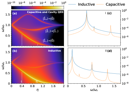
Figure 2: Logarithmic emission spectra obtained for $T_{q}/\omega_{r}=0.1$, $\Delta/\omega_{r}=1$, and $\epsilon=0$. (a) Logarithmic spectrum $S(\omega)$ as a function of $\eta$ and the frequency at the steady state $\hat{\rho}_{ss}$. This emission spectrum concerns the capacitive coupling with the TL and the cavity QED one. (b) On the contrary, this logarithmic spectrum refers to the mutual inductive coupling with the TL. Spectra (a) and (b) are normalized with respect to the maximum value of $S(\omega)$. (c) Logarithmic spectrum as a function of the frequency, $\eta$ is fixed to $0.4$ in this case. (d) Here, the logarithmic spectrum is computed for $\eta=1$. Spectra (c) and (d) are normalized with respect to the maximum value of spectra (a) and (b).

We start analyzing the zero-flux offset case ($\epsilon=0$, implying $\theta=\pi/2$), corresponding to a system described by the standard quantum Rabi model (QRM) Hamiltonian [see Eq. (2)].

We study the non-equilibrium dissipative dynamics of this circuit-QED system under incoherent (thermal-like) excitation. In particular, we solve numerically the steady-state master equation, setting the qubit effective-temperature $T_{q}/\omega_{r}=0.1$. The system incoherent excitation through the qubit reservoir is able to populate the lowest energy excited states of the system $\ket{\tilde{n}_{\pm}}$, which in turn decay towards the lower energy states. In the QRM, beyond the strong-coupling regime, the eigenstates do not exhibit the simple structure of the Jaynes-Cummings (JC) model. Therefore, we use a generalized notation for these states by introducing a tilde [28, 24]. In particular, the system energy states are labelled so that in the small $\eta$ limit $\ket{\tilde{n}_{\pm}}$ coincides with the corresponding JC state $\ket{n_{\pm}}$.

Figure 2(a,b) shows the resulting emission steady-state spectra as a function of the system coupling rate $\eta$. In particular, Fig. 2(a) describes the case of capacitive coupling with the TL, while Fig. 2(b) displays the spectrum obtained for the inductive coupling with the input-output TL. Both panels clearly highlight the transitions $(\tilde{1}_{-},\tilde{0})$, $(\tilde{2}_{-},\tilde{1}_{-})$, and $(\tilde{1}_{+},\tilde{0})$ (in ascending order of frequency). As expected, the $(\tilde{1}_{-},\tilde{0})$ transition line is the most intense for any values of $\eta$ at such low effective temperature, being the lowest energy transition. The other transitions tend to become brighter at increasing coupling strength, until the decoupling fate occurs in the DSC limit [29]. We observe that the mutual inductive spectrum exhibits a quenching of the $(\tilde{1}_{+},\tilde{0})$ spectral line when the coupling ranges roughly from 0.4 to 1 [see Fig. 2(b)]. This different behaviour between the two cases is determined by the matrix elements of the corresponding system observables coupled to the output channels (see Fig. 3). Fig. 2(c, d) display the spectra obtained fixing specific values of the normalized coupling: $\eta=0.4,1$; respectively.

Figure 3 shows the square modulus of the system matrix elements determining the output emission associated to the transitions $\ket{\tilde{1}_{-}}\to|\tilde{0}\rangle$ and $|\tilde{1}_{+}\rangle\to|\tilde{0}\rangle$ versus the normalized coupling strength $\eta$: $\absolutevalue{\bra{\tilde{1}_{-}}\dot{\hat{X}}_{M(C)}\ket{\tilde{0}}}^{2}$ [Fig. 3(a)] and $\absolutevalue{\bra{\tilde{1}_{+}}\dot{\hat{X}}_{M(C)}\ket{\tilde{0}}}^{2}$ [Fig. 3(b)].

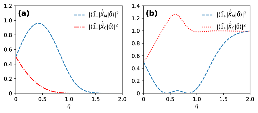
Figure 3: Modulus squared of the matrix elements of the voltage operators $\dot{\hat{X}}_{M}$ and $\dot{\hat{X}}_{C}$ as a function of $\eta$, with $\epsilon=0$ and $\Delta/\omega_{r}=1$.

These results are a clear evidence how the calculated spectra are influenced by the observable coupled to the output port. This influence, however, becomes evident only in the USC or DSC regime. It is also interesting to compare these results for circuit QED systems with the corresponding results for a cavity QED model, where the atomic transition interacts with the cavity field via standard dipolar coupling [24, 30], and where the photodetection rate is proportional to the expectation value of the product of the negative and positive electric-field operators [31]; that is, $\hat{X}_{D}=i(\hat{a}-\hat{a}^{\dagger})-2\eta\,{\hat{\sigma}_{x}}$. It turns out that the dipolar cavity QED spectra coincides with the circuit QED ones computed for the capacitive coupling to the output channel. Looking at the pertinent equations, this can be understood by observing that, applying a phase rotation $\hat{a}\to i\hat{a}$ ($\hat{a}^{\dagger}\to-i\hat{a}^{\dagger}$), to the cavity QED Hamiltonian and to the electric-field operator, the circuit QED Hamiltonian, and the output operator proportional to $\dot{\hat{Q}}$ [see Eq. (10)] are obtained. We can interpret this correspondence, noting that the output capacitive coupling carries on information of the electric field.

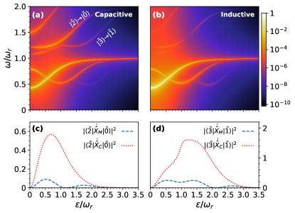
Figure 4: Logarithmic emission spectra setting $T_{q}/\omega_{r}=0.15$, $\Delta/\omega_{r}=1$, and $\eta=0.6$. (a) Logarithmic spectrum $S(\omega)$ as a function of $\epsilon/\omega_{r}$ and the frequency at the steady state $\hat{\rho}_{ss}$. In particular, this emission spectrum concerns the capacitive coupling with the TL. (b) Logarithmic spectrum for the mutual inductive coupling with the TL. Both spectra (a) and (b) are normalized with respect to the maximum value of $S(\omega)$. The spectral lines of our interest are indicated in the panel (a). Panels (c) and (d) show the matrix element of $\dot{\hat{X}}_{C}$ and $\dot{\hat{X}}_{M}$ regarding the transitions displaying peculiar behaviour.

III.2 Symmetry breaking (non-zero flux offset)

Circuit QED systems consisting for example by an LC oscillator interacting with a flux qubit are usually characterized by detecting spectra as a function of the qubit flux offset $\epsilon$ [17, 18, 32]. For $\epsilon\not=0$ the parity selection rule of the standard QRM breaks down and the system can be described by a generalized quantum Rabi model [see Eq. (2)]. In this subsection, we present incoherent emission spectra versus the flux offset $\epsilon$ for a normalized coupling strength $\eta=0.6$. We also consider an effective temperature of the qubit $T_{q}/\omega_{r}=0.15$. Figure 4 displays the evolution (as a function of the flux offset) of several transitions. Note that we have switched the notation of the energy eigenstates from $\ket{\tilde{n}_{\pm}}$ to $\ket{\tilde{n}}$; increasing $n$, the energy grows.

We observe that, also in this case, the lowest transition, $(\tilde{1},\tilde{0})$, is the most dominant for any $\epsilon$ for both the interaction kinds with the TL.

Figure 4(c,d) show the square modulus of the expectation values of the relevant output system operators determining the intensity of two emission lines (associated to the transitions $|\tilde{2}\rangle\to|0\rangle$ and $|\tilde{3}\rangle\to|1\rangle$ ) for the capacitive and inductive coupling to the output channel. As explicitly shown in Fig. 4(c,d), these two transitions are forbidden at $\epsilon=0$. Moreover, we observe that these matrix elements explain the different intensities of the lines highlighted in Fig. 4(a) and Fig. 4(b).

IV Conclusions

We presented a general framework for the calculation of emission spectra in circuit QED systems which is also suitable for systems operating in the USC and DSC regimes. We applied it to calculate emission spectra in a system constituted by a flux qubit coupled to an LC electromagnetic resonator, under incoherent (thermal-like) excitation of the qubit. We find that, even at zero flux offset, when the energy levels correspond to those of the quantum Rabi model for dipolar atomic emitters (cavity QED), the circuit QED spectra may significantly differ from the corresponding cavity QED ones. In particular, we show that the circuit QED spectra can depend on how the resonator is coupled to the output port used for detection. In the case of a resonator capacitively coupled to the output port, cavity QED spectra are recovered in the absence of qubit flux offset.

These results can directly be extended to investigate reflectivity and transmission spectra in circuit QED systems and can provide a more accurate description of experiments concerning the USC regime in circuit QED.

Appendix A Circuits quantization

In this appendix, we conduct the derivation of the circuits Hamiltonian by performing the canonical quantization procedure.

Regarding the capacitive coupling with a semi-infinite transmission line [Fig. 1(b)] and given that choice of nodes, the position of the ground, and according to Ref. [33], the following Lagrangian yields to the corresponding Kirchoff equations of motion:

$$\begin{split}\mathcal{L}_{C}&=\mathcal{L}_{q}+\frac{1}{L}\Phi\Phi_{q}+\frac{1}{2}\,\dot{\underline{{\Phi}}}^{T}\,\underline{\underline{C}}\,\dot{\underline{{\Phi}}}-\frac{\Phi^{2}}{2L}-\frac{(\Phi_{1}-\Phi_{0})^{2}}{2L_{T}}+\\ &+\sum_{i=1}^{\infty}\frac{C_{T}}{2}\dot{\Phi_{i}}^{2}-\sum_{i=1}^{\infty}\frac{(\Phi_{i+1}-\Phi_{i})^{2}}{2L_{T}}\,.\end{split}$$ (13)

A flux qubit is considered, hence $\mathcal{L}_{q}=1/2\;C_{j}\dot{\Phi}^{2}_{q}-\Phi^{2}_{q}/2\tilde{L}+E_{j}\cos[2\pi/\Phi_{0}\;(\Phi_{q}-\Phi_{\rm ext})\bigl{]}$[3], where $\tilde{L}\simeq(L\,L_{C})/(L+L_{C})$ is the equivalent inductance which does not take into account the contribute of the loop inductance $L_{j}$. The relative Hamiltonian is obtained by applying the Legendre transformation:

$$\begin{split}\mathcal{H}_{C}&=\mathcal{H}_{q}+\frac{1}{2C}Q^{2}+\frac{\Phi^{2}}{2L}-\frac{1}{L}\Phi\Phi_{q}+\frac{1}{2C_{T}}Q^{2}_{0}+\\ &+\frac{(\Phi_{1}-\Phi_{0})^{2}}{2L_{T}}+\sum_{i=1}^{\infty}\frac{Q^{2}_{i}}{2C_{T}}+\sum_{i=1}^{\infty}\frac{(\Phi_{i+1}-\Phi_{i})^{2}}{2L_{T}}+\\ &+\frac{C_{K}}{CC_{T}}Q\,Q_{0}\,.\end{split}$$ (14)

Equation 14 would contain convoluted terms regarding the capacitors due to the capacitive coupling with the TL. Under the condition that $C_{K}\ll\{C_{T},C\}$, it can be simplified to that form.

Recalling that

$$\mathcal{{H}}_{q}=\frac{{Q}_{q}^{2}}{2C_{j}}+\frac{{\Phi}^{2}_{q}}{2\tilde{L}}-E_{j}\cos[{\frac{2\,\pi}{\Phi_{0}}}({\Phi}_{q}-\Phi_{\rm ext})\bigl{]}\,,$$ (15)

and

$$\mathcal{{H}}_{LC}=\frac{{Q}^{2}}{2C}+\frac{{\Phi}^{2}}{2L}\,,$$ (16)

the first four terms of Eq. (14) represent the flux gauge Hamiltonian, containing the qubit Hamiltonian, the LC oscillator term, and the coordinate-coordinate (galvanic) interaction [18]. The next four terms constitute the Hamiltonian of the transmission line and the last term can be identified as the interaction Hamiltonian with the TL.

Taking the continuum limit of the TL introduces a flux field $\phi(x)$ and a charge density field $\rho(x)=Q_{n}/\Delta x$ [4]. Now, the canonical quantization can be performed by promoting the canonical variables to operators; that is, $\commutator{\hat{\Phi}}{\hat{Q}}=i$, $\commutator{\hat{\Phi}_{q}}{\hat{Q}_{q}}=i$, and $\commutator{\hat{\phi}(x)}{\hat{\rho}(x^{\prime})}=i\,\delta(x-x^{\prime})$.

Since a semi-infinite transmission line is considered, the charge field operator can be expanded as (see Ref. [13])

$$\hat{\rho}(x)=i\int_{0}^{\infty}d\omega\sqrt{\frac{\omega\,c_{T}}{\pi v_{0}}}\,\cos{\biggl{(}\frac{\omega x}{v_{0}}\biggr{)}}(\hat{b}^{\dagger}_{\omega}-\hat{b}_{\omega}),$$ (17)

thus we recover Eq. (4) and Eq. (5).

Proceeding in the same way, the full Hamiltonian of the mutual inductive coupling with the TL [see Fig. 1(a)] reads as

$$\begin{split}\mathcal{H}_{M}&=\mathcal{H}_{q}+\frac{Q^{2}}{2\,C}+\frac{1}{2\,\tilde{L}}\,\Phi^{2}+\frac{1}{2\,L}(\Phi-\Phi_{q})^{2}+\frac{1}{2\,C_{T}}\times\\ &\times\sum_{j=1}Q^{2}_{j}+\frac{1}{2\tilde{L}_{T}}(\Phi_{n+1}-\Phi_{n})^{2}+\frac{1}{2\,L_{T}}\\ &\times\sum_{j\not=n}(\Phi_{j+1}-\Phi_{j})^{2}+\frac{\Phi-\Phi_{q}}{\tilde{M}}\,(\Phi_{n+1}-\Phi_{n})\,.\end{split}$$ (18)

Now, the last row takes into account the coupling with the TL by means of $\tilde{M}=(L\,L_{T}-M^{2})/M$ (an effective mutual inductance; Ref. [6]). Furthermore, rescaled inductors $\tilde{L}$ and $\tilde{L}_{T}$ are introduced in Eq. (18). The first is equal to $L\,L_{T}-M^{2}/L_{T}$, the latter to $L\,L_{T}-M^{2}/L$. If the aim is to carry out QND (quantum non-destructive) measurements [34, 35], a common design choice consists in taking $M\ll L$, as indicated by Ref. [6]. Under that condition, $\tilde{L}$ and $\tilde{L}_{T}$ can be evaluated with their original values.

Applying the infinite limit of the TL and quantization procedure, the flux field $\hat{\phi}(x)$ operator can be expressed as [30, 4]

$$\hat{\phi}(x)=\int_{0}^{+\infty}d\omega\,\frac{\Lambda}{\sqrt{\omega}}\big{(}\hat{b}_{\omega}\,e^{ikx}+\hat{b}^{\dagger}_{\omega}\,e^{-ikx}\big{)}\,,$$ (19)

where $k=\omega/v_{0}$.

At this point, the interaction Hamiltonian, $\hat{\mathcal{V}}_{M}$, can be expressed as

$$\hat{\mathcal{V}}_{M}=\alpha\hat{\Phi}_{L}\,\int dx\,\delta(x)\frac{\partial\hat{\phi}(x)}{\partial x}\,,$$ (20)

where $\hat{\Phi}_{L}=\hat{\Phi}-\hat{\Phi}_{q}=\Phi_{\rm zpf}\,[\hat{a}+\hat{a}^{\dagger}-2\eta\,(\cos{\theta}\,\hat{\sigma}_{z}-\sin{\theta}\,\hat{\sigma}_{x})]$.

In the end, we find that

$$\hat{\mathcal{V}}_{M}=i\,\frac{1}{\Phi_{\rm zpf}}\,\hat{\Phi}_{L}\int_{0}^{+\infty}d\omega\,\alpha\Phi_{\rm zpf}\,\frac{\Lambda}{v_{0}}\,\sqrt{\omega}\,[\hat{b}_{\omega}-\hat{b}^{\dagger}_{\omega}]\,,$$ (21)

so recovering Eq. (1) and Eq. (3).

Appendix B Generalized Liouvillian

In this appendix, we present the full form of the generalized Liouvillian presented in Eq. (6).

Following the derivation of Ref. [22],

$$\mathcal{L}_{g}\,\hat{\rho} =\frac{1}{2}\sum_{\begin{subarray}{c}i=(r,q)\\ (\omega,\omega^{\prime})>0\end{subarray}}\bigg{\{}\frac{\gamma_{i}\,\omega^{\prime}}{\omega_{i}}\,n_{\rm th}(\omega^{\prime},T_{i})\bigl{[}\hat{A}_{i}^{(-)}(\omega^{\prime})\hat{\rho}(t)\hat{A}_{i}^{(+)}(\omega)$$

$$-\hat{A}_{i}^{(+)}(\omega)\hat{A}_{i}^{(-)}(\omega^{\prime})\hat{\rho}(t)\bigr{]}+\frac{\gamma_{i}\,\omega}{\omega_{i}}\,n_{\rm th}(\omega,T_{i})$$

$$\times\bigl{[}\hat{A}_{i}^{(-)}(\omega^{\prime})\hat{\rho}(t)\hat{A}_{i}^{(+)}(\omega)-\hat{\rho}(t)\hat{A}_{i}^{(+)}(\omega)\hat{A}_{i}^{(-)}(\omega^{\prime})\bigr{]}$$

$$+\frac{\gamma_{i}\,\omega}{\omega_{i}}[n_{\rm th}(\omega,T_{i})+1]\bigl{[}\hat{A}_{i}^{(+)}(\omega)\hat{\rho}(t)\hat{A}_{i}^{(-)}(\omega^{\prime})$$

$$-\hat{A}_{i}^{(-)}(\omega^{\prime})\hat{A}_{i}^{(+)}(\omega)\hat{\rho}(t)\bigr{]}+\frac{\gamma_{i}\,\omega^{\prime}}{\omega_{i}}\,[n_{\rm th}(\omega^{\prime},T_{i})+1]$$

$$\times\bigl{[}\hat{A}_{i}^{(+)}(\omega)\hat{\rho}(t)\hat{A}_{i}^{(-)}(\omega^{\prime})-\hat{\rho}(t)\hat{A}_{i}^{(-)}(\omega^{\prime})\hat{A}_{i}^{(+)}(\omega)\bigr{]}$$

$$+\frac{\gamma_{i}}{\omega_{i}}\,T_{q}\,\mathcal{D}[\hat{\tilde{\sigma}}_{x}^{(0)}]\hat{\rho}(t)+\frac{\gamma_{i}}{\omega_{i}}\,(T_{q}+1)\,\mathcal{D}[\hat{\tilde{\sigma}}_{x}^{(0)}]\hat{\rho}(t)\,,$$ (22)

where $n_{\rm th}(\omega,T_{i})=(e^{{\omega}/{T_{i}}}-1)^{-1}$ represents the mean number of thermal photons; note that with $\omega$ or $\omega^{\prime}$ we indicate a transition frequency of the light-matter system.

The apex in $\hat{A}^{(\pm)}_{i}$ denotes the positive (or negative) frequency component of the corresponding operator written in the diagonal basis of $\mathcal{\hat{H}}_{0}$ [see Eq. (2)]. Using the following relation for a generic system operator

$$\hat{S}^{(0)}=\sum_{i}{S}_{ii}\,\outerproduct{i}{i}\,,$$ (23)

the last row of Eq. (B) pictures the pure dephasing effects associated to the zero-frequency component of $\hat{\tilde{\sigma}}_{x}$, with

$$\mathcal{D}[\hat{\tilde{\sigma}}_{x}^{(0)}]\hat{\rho}=\hat{\tilde{\sigma}}_{x}^{(0)}\hat{\rho}\,\hat{\tilde{\sigma}}_{x}^{(0)}-\frac{1}{2}\hat{\tilde{\sigma}}_{x}^{(0)}\hat{\tilde{\sigma}}_{x}^{(0)}\,\hat{\rho}-\frac{1}{2}\,\hat{\rho}\,\hat{\tilde{\sigma}}_{x}^{(0)}\,\hat{\tilde{\sigma}}_{x}^{(0)}$$ (24)

being the Lindblad dissipator. If the symmetry is not broken ($\epsilon=0$), this term goes to zero.

In Eq. (B), for $i=r$, $\omega_{i}$ corresponds to the LC resonance frequency $\omega_{r}$, whereas, for $i=q$, $\omega_{i}$ is associated to $\Delta$. Moreover, $\hat{A}_{r}=\hat{X}_{C}$, $\hat{A}_{r}=\hat{X}_{M}$, and $\hat{A}_{r}=\hat{X}_{D}$, if we consider the capacitive coupling, the inductive coupling, or the cavity QED case; respectively. Concerning the qubit internal losses, $\hat{A}_{q}=\hat{\tilde{\sigma}}_{x}$ for both circuit schemes, whereas $\hat{A}_{q}=\hat{\sigma}_{x}$ when we deal with the cavity QED dissipation (see Sec. II.1 and Sec. II.2).

In the interaction picture, the first six row terms oscillate at frequencies $\pm(\omega-\omega^{\prime})$. As shown by Ref. [22], if $\pm(\omega-\omega^{\prime})$ is much greater than the damping rates, these terms can be neglected and their numerical computation can give rise to issues that could emerge in the logarithmic spectra . Here, $F(\omega,\omega^{\prime})$ plays the role of a Gaussian numerical filtering:

$$F(\omega,\omega^{\prime})=e^{-\frac{\absolutevalue{\omega-\omega^{\prime}}^{2}}{2b^{2}}}\,.$$ (25)

The generalized master equation can be reconnected to the dressed master equation found in Ref. [28] when $b$ goes to very low values. We underline how the GME is completely valid for quantum optical systems displaying hybrid harmonic-anharmonic energy spectrum and for whatever coupling strength regime, although the Lindblad form is lost.

Appendix C Input-Output theory

In this appendix, we derive the input-output relations in order to see which operator is related to the voltage measured regarding both coupling schemes.

To begin with the infinite TL connected to the qubit-LC system through a mutual inductance, we find that the continuum limit of the Hamiltonian of Eq. (18) reads as

$$\begin{split}\hat{\mathcal{H}}_{M}=&\hat{\mathcal{H}}_{0}+\int dx\left(\frac{\hat{\rho}^{2}_{c}(x)}{2c_{T}}+\frac{(\partial_{x}\hat{\phi})^{2}}{2l_{T}}\right)+\frac{M}{Ll_{T}}\hat{\Phi}_{L}\\ &\times\int\delta(x)\partial_{x}\hat{\phi}\,.\end{split}$$ (26)

Thus, the Heisenberg equations of motion lead to

$$\dot{\hat{\phi}}(x)=\frac{\hat{\rho}(x)}{c_{T}}\,$$ (27)

and

$$\begin{split}\dot{\hat{\rho}}(x)&=\int dx^{\prime}\frac{i}{l_{T}}\partial_{x^{\prime}}\hat{\phi}\commutator{\partial_{x^{\prime}}\hat{\phi}}{\hat{\rho}(x)}+\frac{iM}{Ll_{T}}\delta(x^{\prime})\commutator{\partial_{x^{\prime}}\hat{\phi}}{\hat{\rho}(x)}\\ &=-\int dx^{\prime}\frac{1}{l_{T}}\left(\partial_{x^{\prime}}\hat{\phi}\right)\,\partial_{x^{\prime}}\delta(x^{\prime}-x)+\\ &\;\;\;\,-\int dx^{\prime}\frac{M}{L\,l_{T}}\delta(x^{\prime})\partial_{x^{\prime}}\delta(x^{\prime}-x)\hat{\Phi}_{L}=\\ &=\frac{1}{l_{T}}(\partial^{2}_{x}\hat{\phi})+\frac{M}{Ll_{T}}\delta^{\prime}(x)\hat{\Phi}_{L}\,.\end{split}$$ (28)

Substituting the last equation in Eq. (27), we obtain

$$\ddot{\hat{\phi}}(x)=\frac{\dot{\hat{\rho}}(x)}{c_{T}}=v^{2}_{0}(\partial^{2}_{x}\hat{\Phi})+\frac{M}{c_{T}\,Ll_{T}}\delta^{\prime}(x)\hat{\Phi}_{L}\,,$$ (29)

corresponding in the Fourier space to

$$\biggl{(}k^{2}+\partial^{2}_{x}\biggr{)}\hat{\phi}(x,\omega)=-\frac{M}{v_{0}^{2}\,c_{T}Ll_{T}}\hat{\Phi}_{L}(\omega)\delta^{\prime}(x)\,.$$ (30)

Its solution can be obtained by means of the Green’s functions [36], so

$$\hat{\phi}^{\pm}_{M_{\rm out}}(x,\omega)=\hat{\phi}^{\pm}_{\rm in}(x,\omega)-\biggl{(}\frac{\,M}{2v_{0}l_{T}Lc_{T}}e^{\pm i\,k\absolutevalue{x}}\hat{\Phi}^{\pm}_{L}(\omega)\biggr{)}\,.$$ (31)

Thus,

$$\hat{V}^{\pm}_{M_{\rm out}}(x,\omega)=\hat{V}^{\pm}_{\rm in}(x,\omega)\pm i\omega\,\frac{M}{2L}e^{\pm i\,k\absolutevalue{x}}\,\hat{\Phi}^{\pm}_{L}(\omega)\,.$$ (32)

The last equation can be written in the time domain as

$$\hat{V}^{\pm}_{M_{\rm out}}(x,t)=\hat{V}^{\pm}_{\rm in}(x,t)-\,\frac{M}{2L}\,\dot{\hat{\Phi}}^{\pm}_{L}(x,t)\,,$$ (33)

where

$$\hat{\Phi}^{\pm}_{L}(x,t)=\int_{0}^{\infty}d\omega\,e^{\pm i\,(\omega/v_{0})\absolutevalue{x}}\,\hat{\Phi}^{\pm}_{L}(\omega)e^{\mp i\omega t}\,.$$ (34)

Concerning the capacitive coupling with the semi-infinite transmission line, adopting the quantum network theory and imposing the boundary condition at
x = 0 [4, 37], the output voltage is written as

$$\hat{V}^{\pm}_{C_{\rm out}}(t-x/v_{0})=\hat{V}^{\pm}_{in}(t+x/v_{0})+Z_{0}\frac{C_{K}}{C}\dot{\hat{Q}}^{\pm}(t-x/v_{0})\,.$$ (35)

References

- You and Nori [2011] J. Q. You and F. Nori, Atomic physics and quantum optics using superconducting circuits, Nature 474, 589 (2011).
- Dowling and Milburn [2003] J. P. Dowling and G. J. Milburn, Quantum technology: the second quantum revolution, Philosophical Transactions of the Royal Society of London. Series A: Mathematical, Physical and Engineering Sciences 361, 1655 (2003).
- You and Nori [2005] J. Q. You and F. Nori, Superconducting Circuits and Quantum Information, Physics Today 58, 42 (2005).
- Blais et al. [2021] A. Blais, A. L. Grimsmo, S. M. Girvin, and A. Wallraff, Circuit quantum electrodynamics, Rev. Mod. Phys. 93, 025005 (2021).
- Makhlin et al. [2001] Y. Makhlin, G. Schön, and A. Shnirman, Quantum-state engineering with Josephson-junction devices, Rev. Mod. Phys. 73, 357 (2001).
- Krantz et al. [2019] P. Krantz, M. Kjaergaard, F. Yan, T. P. Orlando, S. Gustavsson, and W. D. Oliver, A quantum engineer’s guide to superconducting qubits, Applied Physics Reviews 6, 021318 (2019).
- Girvin [2014] S. M. Girvin, in Quantum Machines: Measurement and Control of Engineered Quantum Systems: Lecture Notes of the Les Houches Summer School: Volume 96, July 2011 (Oxford University Press, 2014).
- Adhikari et al. [2013] P. Adhikari, M. Hafezi, and J. M. Taylor, Nonlinear Optics Quantum Computing with Circuit QED, Phys. Rev. Lett. 110, 060503 (2013).
- Deppe et al. [2008] F. Deppe, M. Mariantoni, E. P. Menzel, A. Marx, S. Saito, K. Kakuyanagi, H. Tanaka, T. Meno, K. Semba, H. Takayanagi, E. Solano, and R. Gross, Two-photon probe of the Jaynes–Cummings model and controlled symmetry breaking in circuit QED, Nature Physics 4, 686 (2008).
- Niemczyk et al. [2010] T. Niemczyk, F. Deppe, H. Huebl, E. Menzel, F. Hocke, M. Schwarz, J. Garcia-Ripoll, D. Zueco, T. Hümmer, E. Solano et al., Circuit quantum electrodynamics in the ultrastrong-coupling regime, Nature Physics 6, 772 (2010).
- Forn-Díaz et al. [2010] P. Forn-Díaz, J. Lisenfeld, D. Marcos, J. J. García-Ripoll, E. Solano, C. J. P. M. Harmans, and J. E. Mooij, Observation of the Bloch-Siegert Shift in a Qubit-Oscillator System in the Ultrastrong Coupling Regime, Phys. Rev. Lett. 105, 237001 (2010).
- Frisk Kockum et al. [2019] A. Frisk Kockum, A. Miranowicz, S. De Liberato, S. Savasta, and F. Nori, Ultrastrong coupling between light and matter, Nature Reviews Physics 1, 19 (2019).
- Forn-Díaz et al. [2019] P. Forn-Díaz, L. Lamata, E. Rico, J. Kono, and E. Solano, Ultrastrong coupling regimes of light-matter interaction, Rev. Mod. Phys. 91, 025005 (2019).
- Forn-Díaz et al. [2016] P. Forn-Díaz, G. Romero, C. J. P. M. Harmans, E. Solano, and J. E. Mooij, Broken selection rule in the quantum Rabi model, Scientific Reports 6, 26720 (2016).
- Wang et al. [2024] S.-P. Wang, A. Mercurio, A. Ridolfo, Y. Wang, M. Chen, T. Li, F. Nori, S. Savasta, and J. Q. You, Strong coupling between a single photon and a photon pair (2024), arXiv:2401.02738 [quant-ph] .
- Wang et al. [2023] S.-P. Wang, A. Ridolfo, T. Li, S. Savasta, F. Nori, Y. Nakamura, and J. Q. You, Probing the symmetry breaking of a light–matter system by an ancillary qubit, Nature Communications 14, 4397 (2023).
- Yoshihara et al. [2017a] F. Yoshihara, T. Fuse, S. Ashhab, K. Kakuyanagi, S. Saito, and K. Semba, Superconducting qubit–oscillator circuit beyond the ultrastrong-coupling regime, Nature Physics 13, 44 (2017a).
- Yoshihara et al. [2022] F. Yoshihara, S. Ashhab, T. Fuse, M. Bamba, and K. Semba, Hamiltonian of a flux qubit-LC oscillator circuit in the deep–strong-coupling regime, Scientific Reports 12, 6764 (2022).
- Manucharyan et al. [2017] V. E. Manucharyan, A. Baksic, and C. Ciuti, Resilience of the quantum Rabi model in circuit QED, Journal of Physics A: Mathematical and Theoretical 50, 294001 (2017).
- Chiorescu et al. [2004] I. Chiorescu, P. Bertet, K. Semba, Y. Nakamura, C. J. P. M. Harmans, and J. E. Mooij, Coherent dynamics of a flux qubit coupled to a harmonic oscillator, Nature 431, 159 (2004).
- Savasta et al. [2021] S. Savasta, O. Di Stefano, A. Settineri, D. Zueco, S. Hughes, and F. Nori, Gauge principle and gauge invariance in two-level systems, Phys. Rev. A 103, 053703 (2021).
- Settineri et al. [2018] A. Settineri, V. Macrí, A. Ridolfo, O. Di Stefano, A. F. Kockum, F. Nori, and S. Savasta, Dissipation and thermal noise in hybrid quantum systems in the ultrastrong-coupling regime, Phys. Rev. A 98, 053834 (2018).
- Gardiner and Zoller [2004] C. Gardiner and P. Zoller, Quantum noise: a handbook of Markovian and non-Markovian quantum stochastic methods with applications to quantum optics (Springer Science & Business Media, 2004).
- Mercurio et al. [2022] A. Mercurio, V. Macrì, C. Gustin, S. Hughes, S. Savasta, and F. Nori, Regimes of cavity QED under incoherent excitation: From weak to deep strong coupling, Phys. Rev. Res. 4, 023048 (2022).
- [25] A. Mercurio, L. Gravina, and Y.-T. Huang., QuantumToolbox.jl: A Julia package for quantum information and computing, version v0.11.4.
- Johansson et al. [2012] J. Johansson, P. Nation, and F. Nori, QuTiP: An open-source Python framework for the dynamics of open quantum systems, Computer Physics Communications 183, 1760 (2012).
- Johansson et al. [2013] J. Johansson, P. Nation, and F. Nori, QuTiP 2: A Python framework for the dynamics of open quantum systems, Computer Physics Communications 184, 1234 (2013).
- Beaudoin et al. [2011] F. Beaudoin, J. M. Gambetta, and A. Blais, Dissipation and ultrastrong coupling in circuit QED, Phys. Rev. A 84, 043832 (2011).
- De Liberato [2014] S. De Liberato, Light-Matter Decoupling in the Deep Strong Coupling Regime: The Breakdown of the Purcell Effect, Phys. Rev. Lett. 112, 016401 (2014).
- Settineri et al. [2021] A. Settineri, O. D. Stefano, D. Zueco, S. Hughes, S. Savasta, and F. Nori, Gauge freedom, quantum measurements, and time-dependent interactions in cavity QED, Physical Review Research 3 (2021), 10.1103/physrevresearch.3.023079.
- Glauber [1963] R. J. Glauber, The Quantum Theory of Optical Coherence, Phys. Rev. 130, 2529 (1963).
- Yoshihara et al. [2017b] F. Yoshihara, T. Fuse, S. Ashhab, K. Kakuyanagi, S. Saito, and K. Semba, Characteristic spectra of circuit quantum electrodynamics systems from the ultrastrong- to the deep-strong-coupling regime, Phys. Rev. A 95, 053824 (2017b).
- Vool and Devoret [2017] U. Vool and M. Devoret, Introduction to quantum electromagnetic circuits, International Journal of Circuit Theory and Applications 45, 897 (2017).
- Mallet et al. [2009] F. Mallet, F. R. Ong, A. Palacios-Laloy, F. Nguyen, P. Bertet, D. Vion, and D. Esteve, Single-shot qubit readout in circuit quantum electrodynamics, Nature Physics 5, 791 (2009).
- Huang et al. [2020] H.-L. Huang, D. Wu, D. Fan, and X. Zhu, Superconducting quantum computing: a review, Science China Information Sciences 63, 180501 (2020).
- Economou [2006] E. N. Economou, Green’s functions in quantum physics, Vol. 7 (Springer Science & Business Media, 2006).
- Yurke and Denker [1984] B. Yurke and J. S. Denker, Quantum network theory, Phys. Rev. A 29, 1419 (1984).