Heisenberg-Limited Spin-Mechanical Gravimetry

Abstract

Precision measurements of gravitational acceleration, or gravimetry, enable the testing of physical theories and find numerous applications in geodesy and space exploration. By harnessing quantum effects, high-precision sensors can achieve sensitivity and accuracy far beyond their classical counterparts when using the same number of sensing resources. Therefore, developing gravimeters with quantum-enhanced sensitivity is essential for advancing theoretical and applied physics. While novel quantum gravimeters have already been proposed for this purpose, the ultimate sensing precision, known as the Heisenberg limit, remains largely elusive. Here, we demonstrate that the gravimetry precision in a conditional displacement spin-mechanical system increases quadratically with the number of spins: a Heisenberg-limited spin-mechanical gravimeter. In general, the gravitational parameter is dynamically encoded into the entire entangled spin-mechanical probe. However, at some specific times, the mechanical degree of freedom disentangles from the spin subsystem, transferring all the information about the gravitational acceleration to the spin subsystem. Hence, we prove that a feasible spin magnetization measurement can reveal the ultimate gravimetry precision at such disentangling times. Finally, we demonstrate that the proposed system is robust against spin-mechanical coupling anisotropies.

Introduction.— The measurement of gravitational acceleration, gravimetry, is both theoretically and practically crucial. From a fundamental standpoint, gravimeters can aid in testing general relativity Ciufolini et al. (2016); Asenbaum et al. (2020) and detecting deviations from Newtonian gravity Biswas et al. (2012). From a practical viewpoint, gravimeters find extensive applications in geophysics Van Camp et al. (2017); Pearson-Grant et al. (2018); Carbone et al. (2017); van Dam et al. (2017); Romaides et al. (2001), and thanks to satellite missions Iess et al. (2018); Flechtner et al. (2021); Pail (2014); Ebbing et al. (2018); Visser (1999), it is now possible to shed light on planetary gravity fields and the complex dynamics between Earth’s large masses of land, water, and atmospheric interactions.

Massive mechanical objects are excellent testbeds for gravimetry Rademacher et al. (2020); Marson and Faller (1986); Zhong et al. (2022) because their centers-of-mass are inherently subjected to gravitational acceleration and they straightforwardly couple to light and matter systems Treutlein et al. (2014). While atomic interferometry techniques are predominantly employed for gravimetry Janvier et al. (2022); Stray et al. (2022); Freier et al. (2016); Peters et al. (2001); Mcguirk et al. (2002); Bidel et al. (2013); Kritsotakis et al. (2018); Hu et al. (2013), several other high-precision gravimeters have also been investigated. These include optomechanical systems Monteiro et al. (2017, 2020); Armata et al. (2017); Feng et al. (2020); Xiao et al. (2020); Qvarfort et al. (2021, 2018); Johnsson et al. (2016); Geraci and Goldman (2015), ultracold Bose-Einstein condensate systems Abend et al. (2016); Ke et al. (2018); Phillips et al. (2022); Szigeti et al. (2020); Gietka et al. (2019), micro-electro-mechanical systems Middlemiss et al. (2016); Prasad et al. (2022); Mustafazade et al. (2020); Tang et al. (2019); Krishnamoorthy et al. (2008); Liu et al. (2019), and superconducting systems Merlet et al. (2021). Inspired by matter-wave interferometers Scala et al. (2013); Wan et al. (2016), a gravimeter can be devised using a parametric spin-mechanical system Chen and Yin (2018), which can now be implemented with levitated optomechanics Rademacher et al. (2020); Hebestreit et al. (2018); Scala et al. (2013) or potentially in a more compact solid-state platform thanks to spin engineering Wei et al. (2006); Hendrickx et al. (2021). Among the advantages of this parametric coupling are (i) eliminating the need for matching resonance frequencies between the spin and mechanics Treutlein et al. (2014), (ii) the high-fidelity control and read-out of the spin system Jiang et al. (2009); Shields et al. (2015); Rabl et al. (2009), and (iii) conditionally displacing the mechanical state based on known quantities (the coupling strength and its spin component) Scala et al. (2013); Tufarelli et al. (2011); Montenegro et al. (2014) and an unknown quantity (the gravitational acceleration) Scala et al. (2013); Wan et al. (2016). Except for a few instances in gravimetry (e.g., see Ref. Gietka et al. (2019)) where the Heisenberg limit of precision has been predicted, quantum-enhanced gravimetry at the Heisenberg level remains largely unexplored. We address this issue by exploring the precision limits of gravimetry in parametric spin-mechanical systems.

To achieve this goal, we employ quantum estimation theory Degen et al. (2017); Paris (2009), which provides the theoretical framework for quantifying the precision of sensing unknown quantities. Specifically, for a given resource $N$ (such as the number of particles), the sensitivity of measuring an unknown parameter scales as ${\propto}N^{\mu}$ Giovannetti et al. (2011, 2004, 2006); Degen et al. (2017); Braun et al. (2018). Here, $\mu{=}1$ is the standard limit of precision achievable by classical strategies, $\mu{>}1$ signals quantum-enhanced sensitivity, and $\mu{=}2$ is generally known as the Heisenberg limit of precision. Thus, increasing the value of $\mu$ enhances sensitivity for a given resource $N$. Several questions must be addressed for parametric spin-mechanical gravimeters: (i) How can the ultimate gravimetry precision, the Heisenberg limit, be achieved? (ii) Does the Heisenberg limit hold when probing the system partially? (iii) Under which conditions can a feasible measurement attain the Heisenberg limit? (iv) How robust is the sensing procedure in the presence of noise?

In this Letter, we address all the above questions by demonstrating that: (i) the Heisenberg limit can indeed be achieved by spins initialized in the Greenberger-Horne-Zeilinger (GHZ) state; (ii) the gravitational acceleration is solely encoded in the spin degree of freedom after each mechanical oscillator’s cycle; hence, the Heisenberg limit can hold even if probing only the spin subsystem; (iii) at such a cycle, the spin degree of freedom disentangles from the mechanics, and one can probe the spin system using a feasible magnetization measurement basis; and (iv) the system shows robustness in the presence of coupling strength anisotropies. We predict a sensitivity for moderate experimental parameters in the range of $10^{-11}\text{m/s}^{2}$ to $10^{-6}\text{m/s}^{2}$, without relying on free-fall methodologies or ground-state cooling of the mechanical object.

Information metrics.— The uncertainty of an unknown parameter $g$ encoded in a quantum state $\rho_{g}$ is fundamentally lower bounded by the quantum Cramér-Rao inequality Cramér (1999); Rao (1992); Paris (2009):

$$\mathrm{Var}[g]\geq(\nu\mathcal{F})^{-1}\geq(\nu\mathcal{Q})^{-1},$$ (1)

where $\mathrm{Var}[g]$ is the variance of $g$, $\nu$ is the number of measurements, $\mathcal{F}$ is the classical Fisher information (CFI), and $\mathcal{Q}$ is the quantum Fisher information (QFI). The CFI is defined as $\mathcal{F}{=}\sum_{\Upsilon}p(\Upsilon|g)[\partial_{g}\mathrm{ln}p(\Upsilon|g)]^{2}$, where $\partial_{g}{:=}\partial/\partial g$ and $p(\Upsilon|g){=}\mathrm{Tr}[\hat{\Pi}_{\Upsilon}\rho_{g}]$ is the probability of measuring the quantum state $\rho_{g}$ with the positive-operator valued measure (POVM) $\{\hat{\Pi}_{\Upsilon}\}$ with measurement outcome $\Upsilon$. Hence, the CFI yields the achievable precision for a given POVM. The POVM that maximizes the CFI is known as the QFI, $\mathcal{Q}{:=}\max\limits_{\{\hat{\Pi}_{\Upsilon}\}}\mathcal{F}$. Several expressions exist for the QFI Paris (2009). Here, we consider $\mathcal{Q}_{\mathrm{sm}}{=}4\mathbb{R}\text{e}\left[\langle\partial_{g}\psi(\tau)|\partial_{g}\psi(\tau)\rangle{-}|\langle\partial_{g}\psi(\tau)|\psi(\tau)\rangle|^{2}\right]$ for pure states $\rho_{g}{=}\left|\psi(\tau)\right\rangle\left\langle\psi(\tau)\right|$ (the entire spin-mechanical state) and

$$\mathcal{Q}_{\mathrm{spin}}=2\sum_{n,m}\frac{|\langle\lambda_{m}|\partial_{g}\rho_{\mathrm{spin}}|\lambda_{n}\rangle|^{2}}{\lambda_{n}+\lambda_{m}},\hskip 14.22636pt\lambda_{n}+\lambda_{m}\neq 0,$$ (2)

for the reduced density matrix of the spin system, where $\rho_{\mathrm{spin}}{=}\sum_{i}\lambda_{i}|\lambda_{i}\rangle\langle\lambda_{i}|$ is represented in its spectral decomposition, with $\lambda_{i}$ and $|\lambda_{i}\rangle$ being the $i$th eigenvalue and eigenvector of $\rho_{\mathrm{spin}}$, respectively Paris (2009). The QFI quantifies the sensing capability of the quantum probe $\rho_{g}$; thus, a higher QFI value indicates lower uncertainties in $g$, as shown in Eq. (1). Note that the QFI does not explicitly provide the optimal measurement basis, and one needs to build the POVM from the symmetric logarithmic derivative (SLD) operator $L_{g}$ satisfying $2\partial_{g}{\rho_{g}}{=}L_{g}\rho_{g}{+}\rho_{g}L_{g}$ Paris (2009); Liu et al. (2016). In addition, the ultimate precision limit is a consequence of the response of the quantum probe to infinitesimal changes in the vicinity of the unknown parameter Sidhu and Kok (2020); Braunstein and Caves (1994).

The model.— We consider $N$ non-interacting spin-1/2 particles coupled to a single-mode harmonic oscillator via a conditional displacement Hamiltonian:

$$\hat{H}=\frac{1}{2M}\hat{p}^{2}+\frac{M\omega^{2}}{2}\hat{x}^{2}-\sum_{i=1}^{N}\bar{k}_{i}\frac{\hat{\sigma}_{i}^{z}}{2}\hat{x}+\bar{g}M\hat{x}\cos\xi,$$ (3)

where $\hat{p}$ and $\hat{x}$, satisfying $[\hat{x}{,}\hat{p}]{=}i\hbar$, are the momentum and position operators of a mechanical object with mass $M$ and frequency $\omega$, respectively. $\hat{\sigma}_{i}^{\beta}$, $\beta{=}x{,}y{,}z$, is the Pauli operator for the $i$th spin, which interacts with the mechanical oscillator with strength $\bar{k}_{i}$. The final term describes the gravitational potential energy Qvarfort et al. (2018); Scala et al. (2013); Armata et al. (2017); Chen and Yin (2018), where $\bar{g}$ is the gravitational acceleration, and $\xi$ is the angle between the $x-$direction and the free fall acceleration Qvarfort et al. (2018); Scala et al. (2013). The Hamiltonian for a single spin interacting with a mechanical oscillator, in the absence of the gravitational term, has been extensively investigated Khosla et al. (2018); Rabl et al. (2010, 2009); Rabl (2010); Braccini et al. (2023); Rao et al. (2016); Montenegro et al. (2017); Tufarelli et al. (2012); Montenegro et al. (2018); Tufarelli et al. (2011); Scala et al. (2013); Montenegro et al. (2014); Yin et al. (2013); Spiller et al. (2006); Kumar and Bhattacharya (2017). By introducing $\hat{p}{=}i\sqrt{M\hbar\omega/2}(\hat{a}^{\dagger}{-}\hat{a})$ and $\hat{x}{=}\sqrt{\hbar/(2M\omega)}(\hat{a}^{\dagger}{+}\hat{a})$, one can write Eq. (3) as follows:

$$\frac{\hat{H}}{\hbar\omega}{=}\hat{a}^{\dagger}\hat{a}{-}\hat{Z}(\bm{k}{,}g)\left(\hat{a}^{\dagger}{+}\hat{a}\right),$$ (4)

where $\hat{Z}(\bm{k}{,}g){:=}\left[\sum\limits_{i=1}^{N}k_{i}\frac{\hat{\sigma}_{i}^{z}}{2}{-}g\right]$ is a spin operator depending on the coupling strengths $\bm{k}{=}{\{k_{i}\}}$ and the unknown parameter $g$ to be estimated. Moreover, we have defined the quantities $\hbar k_{i}{:=}\bar{k}_{i}\sqrt{\hbar/(2M\omega^{3})}$, $\hbar g{:=}\bar{g}\sqrt{M\hbar/(2\omega^{3})}\cos\xi$. We will set $\xi{=}0$ from this point forward. To solve the quantum dynamics, it has been analytically derived the unitary temporal operator for Eq. (4) as Montenegro et al. (2014):

$$\hat{U}(\tau){=}e^{i\hat{Z}(\bm{k}{,}g)^{2}(\tau{-}\sin\tau)}e^{\hat{Z}(\bm{k}{,}g)(\eta(\tau)\hat{a}^{\dagger}{-}\eta^{*}(\tau)\hat{a})}e^{-i\hat{a}^{\dagger}\hat{a}\tau},$$ (5)

where $\eta(\tau){:=}1{-}e^{-i\tau},$ and $\tau{:=}\omega t$. Thanks to mechanical oscillators’ current ground state cooling O’Connell et al. (2010), we will initialize the mechanical object in a coherent state $|\alpha\rangle$, $\alpha{\in}\mathbb{R}$. This is not a limitation, as the spin-mechanical gravimeter used here operates effectively even when the mechanical oscillators are initially in a thermal state, see Supplemental Material (SM) for details SM . Conversely, depending on the sensing case, the spin state will be initialized differently. Note that at $\tau$ multiples of $2\pi$, the unitary operator $\hat{U}(\tau{=}2\pi)$ acquires relative phases for the spin states ${\propto}e^{2\pi i\hat{Z}(\bm{k}{,}g)^{2}}$, whereas the coherent field returns to its initial state $|\alpha\rangle$. For $0{<}\tau{<}2\pi$, the mechanical state rotates in phase-space by an angle $\tau$ due to $e^{-i\hat{a}^{\dagger}\hat{a}\tau}$, and it is conditionally displaced by the spin state by an amount ${\propto}\langle\hat{Z}(\bm{k},g)\rangle\eta(\tau)$. Here, $\langle\cdot\rangle$ is the expected value concerning a spin state. In what follows, we will investigate the precision limits of gravimetry for equal-scaled spin-mechanical coupling $k_{i}{=}k_{j},\forall i{,}j$. The scenario where $k_{i}{\neq}k_{j},\forall i{,}j$ will be addressed later.

Elemental gravimetry scenarios.— Two straightforward scenarios can be explored: (i) a single spin and (ii) two spins coupled to the mechanical oscillator. The former, initialized as $|\psi(0)\rangle{=}\frac{1}{\sqrt{2}}(|0\rangle{+}|1\rangle)|\alpha\rangle$, yields a QFI (see SM for details SM ):

$$\mathcal{Q}_{\mathrm{sm}}^{(1)}\propto k^{2}(\tau-\sin\tau)^{2}-2\cos\tau.$$ (6)

For the two spins scenario, we initialized the spins in their computational basis: $|\psi(0)\rangle_{\mathrm{spin}}^{(2)}{=}R_{1}|01\rangle{+}R_{2}|00\rangle{+}R_{3}|10\rangle{+}R_{4}|11\rangle$, with $R_{j}{=}r_{j}e^{i\phi_{j}}$ and $\sum\limits_{j{=}1}^{4}|R_{j}|^{2}{=}1$. Giving the QFI (see SM SM for details):

$$\mathcal{Q}_{\mathrm{sm}}^{(2)}{\propto}8k^{2}[r_{4}^{2}{-}r_{4}^{4}{-}r_{2}^{4}{+}r_{2}^{2}(1{+}2r_{4}^{2})](\tau{-}\sin\tau)^{2}{-}4\cos\tau.$$ (7)

Maximizing Eq. (7) over the values of $r_{2}$ and $r_{4}$ yields $r_{2}{=}r_{4}{=}1/\sqrt{2}$. Hence, the triplet state $\sqrt{2}|\psi(0)\rangle_{\text{spin}}^{(2)}{=}(|00\rangle{+}|11\rangle)$ Chen and Yin (2018) gives rise to $\mathcal{Q}_{\text{sm}}^{(2)}{\propto}4k^{2}(\tau{-}\sin\tau)^{2}{-}2\cos\tau$, which can be interpreted as the single spin scenario with an effective coupling of $2k$. As experimental constraints limit the coupling strength, adding more spins can alleviate this restriction. The enhancement in gravimetry precision from the triplet state motivates us to explore the ultimate limits of gravimetry precision with $N$ spins.

Heisenberg-limited gravimetry.— We introduce the collective spin operator $\hat{S}_{\beta}{=}\sum\limits_{i{=}1}^{N}\frac{\hat{\sigma}_{i}^{\beta}}{2}$. Fulfilling: $[\hat{S}_{n}{,}\hat{S}_{m}]{=}i\hbar\varepsilon_{nml}\hat{S}_{l}$, $\hat{S}^{2}|s{,}m\rangle{=}\hbar^{2}s(s{+}1)|s{,}m\rangle$ and $\hat{S}_{z}|s{,}m\rangle{=}\hbar m|s{,}m\rangle$. In the above, $\varepsilon_{nml}$ is the Levi-Civita symbol, $s{\leq}N{/}2$ is the spin number, and ${-}s{\leq}m{\leq}s$ is the angular momentum’s component along the $z$-direction ($|m|{\leq}s$). With this notation, $\hat{Z}(\bm{k}{,}g){=}k\hat{S}_{z}{-}g$. By considering the symmetric case, namely $2s{=}N$, and an initial spin-mechanical state $\left|\psi(0)\right\rangle{=}\sum\limits_{m{=}-N/2}^{N/2}c_{m}|\frac{N}{2}{,}m\rangle\left|\alpha\right\rangle$, we obtain the spin-mechanical evolved state:

$$\left|\psi(t)\right\rangle_{\mathrm{sm}}{=}\sum\limits_{m{=}-\frac{N}{2}}^{\frac{N}{2}}\tilde{C}_{m}\left|\frac{N}{2}{,}m\right\rangle\left|\varphi(m{,}g)\right\rangle,$$ (8)

where $\tilde{C}_{m}{:=}c_{m}e^{imk[(\tau{-}\sin\tau)(km{-}2g){+}\alpha\sin\tau]}$, and the mechanical amplitude $\varphi(m{,}g){:=}\alpha e^{-i\tau}{+}(km{-}g)\eta(\tau)$ is conditionally displaced by a quantity $(km{-}g)\eta(\tau)$. The wave function of Eq. (8) is general. In particular, for the Greenberger-Horne-Zeilinger (GHZ) state ($m{=}\pm\frac{N}{2}$):

$$\left|\psi(0)\right\rangle_{\mathrm{spin}}^{(\text{GHZ})}{=}\frac{1}{\sqrt{2}}\left(\left|\frac{N}{2}{,}\frac{N}{2}\right\rangle{+}\left|\frac{N}{2}{,}-\frac{N}{2}\right\rangle\right),$$ (9)

the QFI is found to be, see SM SM for details:

$$\mathcal{Q}_{\mathrm{sm}}^{(\text{GHZ})}{\propto}k^{2}N^{2}(\tau{-}\sin\tau)^{2}{-}2\cos\tau.$$ (10)

Eq. (10) demonstrates that the spin-mechanical probe scales quadratically with the number of particles $N$ for any given time, i.e., it reaches the Heisenberg limit for gravimetry precision. Note that this result is non-trivial. In phase-like sensing tasks with Hamiltonian $\hat{H}{=}\Xi\hat{h}_{0}$, where $\hat{h}_{0}$ is a Hermitian generator Paris (2009) and $\Xi$ is a unknown parameter to be estimated, the GHZ state has been established as the optimal choice for achieving the Heisenberg limit Giovannetti et al. (2004). However, for quantum probes governed by general Hamiltonian $\hat{H}{\neq}\Xi\hat{h}_{0}$, the optimal state will depend on the sensing task Zwierz et al. (2010); Fiderer et al. (2019). Interestingly, Eq. (10) resembles the single spin scenario with an amplified effective spin-mechanical coupling strength of $kN$. To demonstrate this, in Fig. 1(a), we plot the QFI of the spin-mechanical system $\mathcal{Q}_{\mathrm{sm}}$ as a function of time $\tau$ for several values of $kN$. As the figure shows, the $\mathcal{Q}_{\mathrm{sm}}$ benefits from increasing $kN$. For values of $kN{\lesssim}0.1$, the $\mathcal{Q}_{\mathrm{sm}}$ peaks around $\tau{\sim}\pi$, where the spins are highly entangled with the field Montenegro et al. (2014). Thus, the gravitational information $g$ is encoded in the entire correlated state. On the other hand, for $kN{\gtrsim}1$, $\mathcal{Q}_{\mathrm{sm}}$ peaks at $\tau{\rightarrow}2\pi$, where the field disentangles from the spins. Consequently, all information regarding gravitational acceleration $g$ is encoded in the spins subsystem. These facts can be observed from the linear entropy $S_{L}$ (see SM SM for details):

$$S_{L}{=}\left(1{-}e^{2k^{2}N^{2}(\cos\tau{-}1)}\right)/2.$$ (11)

Although entangled states are typically invoked to achieve quantum-enhanced sensitivity Degen et al. (2017); Montenegro et al. (2024), in this case, it is the spin-mechanical disentanglement that transfers all the information about $g$ to the spin state. In Fig. 1(b), we plot the $\mathcal{Q}_{\mathrm{sm}}$ as a function of $(kN)^{2}$ for several times $\tau$. As the figure shows, $\mathcal{Q}_{\mathrm{sm}}$ increases quadratically for any given time.

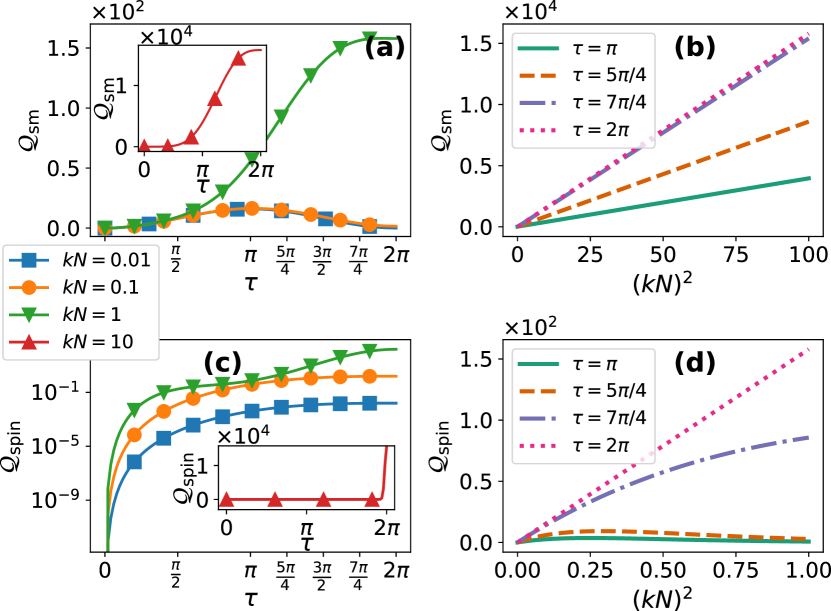
Figure 1: (a) Quantum Fisher information (QFI) of the spin-mechanical system $\mathcal{Q}_{\mathrm{sm}}$ as a function of time $\tau$ for several values of $kN$. (b) $\mathcal{Q}_{\mathrm{sm}}$ as a function of $(kN)^{2}$ for several times $\tau$. (c) QFI of the spin system $\mathcal{Q}_{\mathrm{spin}}$ as a function of time $\tau$ for several values of $kN$. (d) $\mathcal{Q}_{\mathrm{spin}}$ as a function of $(kN)^{2}$ for several times $\tau$.

Heisenberg-limited spin gravimeter.— Probing the entire system can be practically challenging Montenegro et al. (2022). Hence, we explore the gravimetry precision limits for the spin subsystem. As shown in the SM SM , the QFI of the spin subsystem is:

$$\mathcal{Q}_{\mathrm{spin}}{=}4e^{2k^{2}N^{2}(\cos\tau{-}1)}k^{2}N^{2}(\tau{-}\sin\tau)^{2}.$$ (12)

Note that at $\tau$ multiples of $2\pi$, $\mathcal{Q}_{\mathrm{spins}}{\propto}k^{2}N^{2}\tau^{2}$ and the spin subsystem reaches the Heisenberg limit of precision, acquiring all the information regarding $g$, while the mechanical oscillator returns to its initial state $\left|\alpha\right\rangle$. To illustrate this in detail, in Fig. 1(c), we plot $\mathcal{Q}_{\mathrm{spin}}$ as a function of time $\tau$ for different values of $kN$. The figure reveals two key features: (i) $\mathcal{Q}_{\mathrm{spin}}$ always peaks at $\tau$ multiples of $2\pi$, and (ii) as $kN$ increases, $\mathcal{Q}_{\mathrm{spin}}$ becomes vanishingly small, except at $\tau{\rightarrow}2\pi$ [see inset of Fig. 1(c)]. Indeed, in Fig. 1(d), we plot $\mathcal{Q}_{\mathrm{spin}}$ as a function of $(kN)^{2}$ for various choices of times $\tau$. As depicted in the figure, only at $\tau{=}2\pi$ the $\mathcal{Q}_{\mathrm{spin}}$ exhibits the Heisenberg limit. For other values of $\tau$, $\mathcal{Q}_{\mathrm{spins}}$ decreases exponentially by the positive function $e^{2k^{2}N^{2}(\cos\tau{-}1)}$ as $kN$ increases, thereby losing the Heisenberg limit of precision. Two important points need clarification: (i) the failure to tune (or prepare the probe Kacprowicz et al. (2010)) to the parameter that achieves the Heisenberg limit of precision, here $\tau{=}2\pi$, is a common challenge in local quantum sensing Rams et al. (2018); Montenegro et al. (2021); and (ii) losing the Heisenberg limit of precision should not be confused with losing quantum advantage altogether. To illustrate this, we examine the gravimetry precision limits for both a classical and a quantum probe in the vicinity of $\tau{=}2\pi$, where the quantum probe still outperforms the classical one. See SM SM for details.

Classical Fisher information.— The optimal measurement, obtained from the SLD $L_{g}$, for attaining the QFI of the entire system is generally challenging and sometimes infeasible. Therefore, identifying a measurement of a subsystem that extracts the most information content about the unknown parameter is crucial. Let us construct the probability distributions needed for evaluating the CFI for the spin subsystem with POVM $\hat{\Pi}_{\Upsilon}{=}|\Upsilon(\Theta,\Phi)\rangle\langle\Upsilon(\Theta,\Phi)|$, where $|\Upsilon(\Theta,\Phi)\rangle{=}\cos\frac{\Theta}{2}\left|\frac{N}{2},\frac{N}{2}\right\rangle{+}\sin\frac{\Theta}{2}e^{-i\Phi}\left|\frac{N}{2}{,}{-}\frac{N}{2}\right\rangle$. With this choice of spin POVM, $\Upsilon$ can take two measurement outcomes, and the optimal CFI is (see SM SM for its analytical expression):

$$\mathcal{F}_{\mathrm{spin}}{=}\max_{\{\Theta,\Phi\}}\left[\frac{\left[\partial_{g}p(\Upsilon(\Theta{,}\Phi)|g)\right]^{2}}{p(\Upsilon(\Theta{,}\Phi)|g)[1{-}p(\Upsilon(\Theta{,}\Phi)|g)]}\right],$$ (13)

where $p(\Upsilon(\Theta{,}\Phi)|g){=}\left\langle\psi(\tau)\right|\hat{\Pi}_{\Upsilon}\left|\psi(\tau)\right\rangle$ is the probability associated to $\hat{\Pi}_{\Upsilon}$. Maximization analysis shows that $\Theta{=}\frac{\pi}{2}$, while $\Phi$ takes other values. Note that projective measurements of the type $\{\hat{\Pi}_{\Upsilon}\}$ have been proposed for verifying GHZ states Zhao et al. (2021), and the evaluation of the magnetization function through measurements of individual particles has been successfully performed in experiments Wang et al. (2009); Monroe et al. (2021); Islam et al. (2011, 2013); Richerme et al. (2013); Lee et al. (2016); Mooney et al. (2021). In Fig. 2(a), we plot the spin QFI $\mathcal{Q}_{\mathrm{spin}}$ and the spin CFI $\mathcal{F}_{\mathrm{spin}}$ as a function of time $\tau$ for several choices of $kN$. As the figure shows, the choice of the POVM $\hat{\Pi}_{\Upsilon}$ optimized over the angles $\{\Theta{,}\Phi\}$ saturates the QFI of the spin subsystem. Remarkably, for the specific case of $\tau{=}2\pi$, $\hat{\Pi}_{\Upsilon}$ also saturates the QFI of the entire spin-mechanical system. Hence, it constitutes the optimal measurement basis at $\tau{=}2\pi$, achieving the Heisenberg gravimetry precision limit. To quantify the sensing performance of probing the spin subsystem relative to the entire spin-mechanical system for times $\tau{\neq}2\pi$, in Fig. 2(b), we plot the ratio $\mathcal{F}_{\mathrm{spin}}{/}\mathcal{Q}_{\mathrm{sm}}{\leq}1$ as a function of time $\tau$ for several choices of $kN$. The figure reveals two key observations: (i) The information fraction from the spin subsystem is notably low for times $0{<}\tau{\lesssim}2\pi$ in the extreme cases of $kN{\ll}1$ and $kN{\gg}1$ [in agreement with Eq. (12)], and (ii) all information about $g$ becomes codified in the spin subsystem as the field dynamically disentangles from the spin, with $\mathcal{F}_{\mathrm{spin}}{=}\mathcal{Q}_{\mathrm{sm}}$ for the separable spin-mechanical state at $\tau{=}2\pi$. This suggests that there is an optimal value of $kN$ that maximizes the ratio $\mathcal{F}_{\mathrm{spin}}{/}\mathcal{Q}_{\mathrm{sm}}$ in the vicinity of $\tau{=}2\pi$. The above analysis assumes access to the spin subsystem only. For details on uncorrelated measurements performed on the mechanical mode, see SMSM .

Figure 2: (a) Spin QFI $\mathcal{Q}_{\mathrm{spin}}$ and the spin CFI $\mathcal{F}_{\mathrm{spin}}$ as a function of time $\tau$ for several choices of $kN$. (b) Ratio $\mathcal{F}_{\mathrm{spin}}{/}\mathcal{Q}_{\mathrm{sm}}$ as a function of time $\tau$ for several choices of $kN$.

Robustness.— We now investigate the quantum probe robustness in the presence of unequal spin-mechanical coupling strengths $k_{i}{\neq}k_{j},\forall i{,}j$. We simulate the dynamics under $\hat{Z}(\bm{k}{,}g){:=}\left[\sum\limits_{i=1}^{N}k_{i}\frac{\sigma_{i}^{z}}{2}{-}g\right]$ starting from $\sqrt{2}\left|\psi(0)\right\rangle_{\mathrm{sm}}{=}(\left|0\right\rangle^{\otimes N}{+}\left|1\right\rangle^{\otimes N})\left|\alpha\right\rangle$. Each coupling strength fluctuates randomly around a central value $k_{i}$, with $k_{i}{\rightarrow}k_{i}(1{+}\Delta k_{i})$, where $\Delta k_{i}$ is a random number in the interval $[-\delta k{,}\delta k]$. In Fig. 3(a), we plot the average QFI over 1000 instances $\overline{\mathcal{Q}_{\mathrm{sm}}}$ as a function of $N^{2}$ for several random amplitudes $\delta k$. As seen in the figure, the Heisenberg gravimetry precision holds on average. However, in Fig. 3(b), we plot the ratio between the standard deviation $\mathrm{std}[\mathcal{Q}_{\mathrm{sm}}]$ (from sampling 1000 instances) and the average $\overline{\mathcal{Q}_{\mathrm{sm}}}$ as a function of $N$ for several choices of $\delta k$. Ideally, one wants $\mathrm{std}[\mathcal{Q}_{\mathrm{sm}}]{\ll}\overline{\mathcal{Q}_{\mathrm{sm}}}$. The figure shows strong statistical deviations from $\overline{\mathcal{Q}_{\mathrm{sm}}}$ as $\delta k$ increases. Remarkably, these deviations decrease as $N$ increases for a fixed $\delta k$. Thus, with unequal random spin-mechanical coupling strengths, gravimetry precision maintains the Heisenberg limit but faces increased uncertainty in standard deviation as the random amplitude $\delta k$ grows.

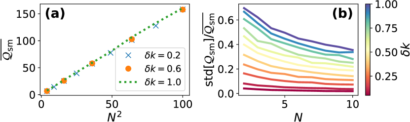
Figure 3: (a) average QFI $\overline{\mathcal{Q}_{\mathrm{sm}}}$ as a function of $N^{2}$ for several choices of $\delta k$. (b) Standard deviation $\mathrm{std}[\mathcal{Q}_{\mathrm{sm}}]$ divided by $\overline{\mathcal{Q}_{\mathrm{sm}}}$ as a function of $N$ for several choices of $\delta k$.

Experimental feasibility.— Several experimental ingredients have been achieved that could potentially be used to implement this proposal. These include: a single spin coupled parametrically to a mechanical oscillator has been demonstrated experimentally Kolkowitz et al. (2012); Arcizet et al. (2011); LaHaye et al. (2009); Martinetz et al. (2020), whereas other hybrid tripartite architectures have also been realized Pirkkalainen et al. (2013); Aporvari and Vitali (2021); Pirkkalainen et al. (2015). On the other hand, mechanical oscillators have been cooled to their ground state Gieseler et al. (2012); Li et al. (2011); O’Connell et al. (2010); Cattiaux et al. (2021), enabling coherent state initialization. Typical mechanical frequencies of the fundamental mode range from $\omega/2\pi{\approx}50\text{MHz}$ with coupling strength $k/2\pi{\approx}0.6{-}4.6\text{MHz}$ LaHaye et al. (2009) to $\omega/2\pi{\approx}80\text{kHz}$ with coupling strength $k/2\pi{\approx}20\text{Hz}$ Kolkowitz et al. (2012). The most challenging step for the spin-mechanical proposal is the GHZ initialization of the spin subsystem. Recent theoretical proposals address this Wei et al. (2006); de Moraes Neto et al. (2017), and high-fidelity 2000-atom GHZ states have been proposed Zhao et al. (2021), along with few-to-14 trapped ions Friis et al. (2018); Leibfried et al. (2004); Monz et al. (2011); Roos et al. (2004); Sackett et al. (2000), 10-qubit superconducting qubits Song et al. (2017), 7-qubit GHZ states in a solid-state spin register Bradley et al. (2019), superconducting transmon qutrits Cervera-Lierta et al. (2022), and three-qubit NMR systems Ji et al. (2019). This work shows a predicted sensitivity for moderate experimental parameters, ranging from $\Delta\bar{g}{\sim}10^{-11}m{/}s^{2}{-}10^{-6}m{/}s^{2}$ for $N{=}2$, see SM SM .

Conclusions.— In this Letter, we prove that the sensitivity of gravimetry can increase quadratically with the number of spins in a conditional displacement spin-mechanical system, sensing performance known as the Heisenberg limit of precision. We show that during each mechanical cycle, the information content of the gravitational acceleration is entirely transferred to the spin subsystem. This phenomenon, resulting from the parametric interaction of the spin-mechanical probe, enables us to identify the optimal measurement basis for achieving the Heisenberg limit by only probing the spin subsystem. Finally, we demonstrate that the proposed scheme is robust against spin-mechanical coupling anisotropies and that our work could potentially compete with other proposals, without relying on free-fall-based methodologies or the need for mechanical ground-state cooling.

Acknowledgements.— V.M. acknowledges support from the National Natural Science Foundation of China (Grants No. 12050410251 and No. 12374482). V.M. would like to thank George Mihailescu and Chiranjib Mukhopadhyay for their useful comments and discussions.

Supplemental Material: Heisenberg-Limited Spin-Mechanical Gravimetry

This Supplemental Material includes analytical expressions for the quantum Fisher information in the following scenarios: the single-spin case, the two-spin case, the Greenberger-Horne-Zeilinger (GHZ) case for the entire spin-mechanical system, and the GHZ case specifically for the spin subsystem. Additionally, we demonstrate that this gravimetry proposal does not require cooling of the mechanical oscillator to its ground state. We also show the system’s entanglement. We evaluate the gravimetry performance when probing the mechanical state using homodyne, heterodyne, and photocounting measurements while optimally measuring the spin. Furthermore, we provide the analytical expression for the classical Fisher information of the reduced density matrix of the spin subsystem. Finally, we assess the robustness of the gravimetry protocol near $\tau=2\pi$ and quantify the predicted gravimetry sensitivity.

I I. Single spin quantum Fisher information

For a single spin coupled to a mechanical harmonic oscillator, the unitary operator reads as:

$$\hat{U}(\tau) =e^{i(\frac{k}{2}\hat{\sigma}^{z}-g\cos\xi)^{2}[\tau-\sin\tau]}e^{(\frac{k}{2}\hat{\sigma}^{z}-g\cos\xi)(\eta(\tau)\hat{a}^{\dagger}-\eta(\tau)^{*}\hat{a})}e^{-i\hat{a}^{\dagger}\hat{a}\tau},$$ (S1)

$$=e^{i(\frac{k}{4}^{2}-2g\frac{k}{2}\cos\xi\hat{\sigma}^{z}+g^{2}\cos^{2}\xi)[\tau-\sin\tau]}e^{(\frac{k}{2}\hat{\sigma}^{z}-g\cos\xi)(\eta(\tau)\hat{a}^{\dagger}-\eta(\tau)^{*}\hat{a})}e^{-i\hat{a}^{\dagger}\hat{a}\tau},$$ (S2)

$$=e^{-2ig\cos\xi\frac{k}{2}\hat{\sigma}^{z}[\tau-\sin\tau]}e^{(\frac{k}{2}\hat{\sigma}^{z}-g\cos\xi)(\eta(\tau)\hat{a}^{\dagger}-\eta(\tau)^{*}\hat{a})}e^{-i\hat{a}^{\dagger}\hat{a}\tau},$$ (S3)

where we have used $\eta(\tau)=1-e^{-i\tau}$ and $\omega t=\tau$. For the initial state (we recall $\hat{\sigma}^{z}=\left|0\right\rangle\left\langle 0\right|-\left|1\right\rangle\left\langle 1\right|$):

$$|\psi(0)\rangle_{\mathrm{sm}}=\left(\cos\frac{\theta}{2}|0\rangle+\sin\frac{\theta}{2}e^{-i\phi}|1\rangle\right)\otimes|\alpha\rangle,$$ (S4)

one gets:

$$|\psi(\tau)\rangle = \cos\frac{\theta}{2}e^{-igk(\tau-\sin\tau)}e^{i\alpha(\frac{k}{2}-g\cos\xi)\sin\tau}e^{-\frac{1}{2}|\alpha e^{-i\tau}+(\frac{k}{2}-g)\eta(\tau)|^{2}}\sum_{n=0}^{\infty}\frac{\left[\alpha e^{-i\tau}+(\frac{k}{2}-g)\eta(\tau)\right]^{n}}{\sqrt{n!}}|0\rangle|n\rangle$$ (S5)

$$+ \sin\frac{\theta}{2}e^{-i\phi}e^{igk(\tau-\sin\tau)}e^{-i\alpha(\frac{k}{2}+g\cos\xi)\sin\tau}e^{-\frac{1}{2}|\alpha e^{-i\tau}-(\frac{k}{2}+g)\eta(\tau)|^{2}}\sum_{n^{\prime}=0}^{\infty}\frac{\left[\alpha e^{-i\tau}-(\frac{k}{2}+g)\eta(\tau)\right]^{n^{\prime}}}{\sqrt{n^{\prime}!}}|1\rangle|n^{\prime}\rangle.$$ (S6)

To evaluate the quantum Fisher information, we compute:

$$\langle\partial_{g}\psi(\tau)|\partial_{g}\psi(\tau)\rangle{=}\frac{1}{2}\cos^{2}\xi\left[4\alpha^{2}-\left(4\alpha^{2}{+}k^{2}\right)\cos(2\tau)-4k\sin\tau\{2\alpha(\sin\tau-\tau)\cos\theta+k\tau\}+2k^{2}\tau^{2}+k^{2}-4\cos\tau+4\right],$$ (S7)

and

$$|\langle\partial_{g}\psi(\tau)|\psi(\tau)\rangle|^{2}=\cos^{2}\xi(2\alpha\sin\tau+k(\tau-\sin\tau)\cos\theta)^{2}.$$ (S8)

Therefore, the quantum Fisher information of the entire spin-mechanical system is:

$$\mathcal{Q}_{\mathrm{sm}} = 4\mathbb{R}\text{e}\left[\langle\partial_{g}\psi(\tau)|\partial_{g}\psi(\tau)\rangle-|\langle\partial_{g}\psi(\tau)|\psi(\tau)\rangle|^{2}\right]$$ (S9)

$$= \cos^{2}\xi\left(k^{2}\left(2\tau^{2}+1\right)+k^{2}\left[-2(\tau-\sin\tau)^{2}\cos(2\theta)-4\tau\sin\tau-\cos(2\tau)\right]-8\cos\tau+8\right).$$ (S10)

From the above, the optimal probe is given by $\theta=\frac{\pi}{2}$, which results in $|\psi(0)\rangle_{\mathrm{sm}}=\frac{1}{\sqrt{2}}\left(|0\rangle+e^{-i\phi}|1\rangle\right)|\alpha\rangle$ with an irrelevant $\phi$ angle. This leads to the optimal probe shown in the main text, $|\psi(0)\rangle_{\mathrm{sm}}=\left|+\right\rangle|\alpha\rangle$. Hence:

$$\mathcal{Q}_{\mathrm{sm}} = k^{2}\left(2\tau^{2}+1\right)+k^{2}\left[-2(\tau-\sin\tau)^{2}\cos(2\theta)-4\tau\sin\tau-\cos(2\tau)\right]-8\cos\tau+8,$$ (S11)

$$= k^{2}\left(4\tau^{2}+2\right)-2k^{2}\left[4\tau\sin\tau+\cos(2\tau)\right]-8\cos\tau+8,$$ (S12)

$$\propto k^{2}(\tau-\sin\tau)^{2}-2\cos\tau.$$ (S13)

The above quantum Fisher information of the entire system is the one presented in the main text; see Eq. (6).

II II. Two spins quantum Fisher information

Similarly to the single spin case shown above, we first explicitly derive the unitary temporal operator for two spins as follows:

$$\hat{U}(\tau) =e^{i\left(\frac{k_{1}}{2}\hat{\sigma}_{1}^{z}+\frac{k_{2}}{2}\hat{\sigma}_{2}^{z}-g\cos\xi\right)^{2}[\tau-\sin\tau]}e^{\left(\frac{k_{1}}{2}\hat{\sigma}_{1}^{z}+\frac{k_{2}}{2}\hat{\sigma}_{2}^{z}-g\cos\xi\right)(\eta(\tau)a^{\dagger}-\eta(\tau)^{*}a)}e^{-ia^{\dagger}a\tau},$$ (S14)

$$=e^{i(2\frac{k_{1}}{2}\frac{k_{2}}{2}\hat{\sigma}_{1}^{z}\hat{\sigma}_{2}^{z}-2\frac{k_{1}}{2}g\cos\xi\hat{\sigma}_{1}^{z}-2\frac{k_{2}}{2}g\cos\xi\hat{\sigma}_{2}^{z})[\tau-\sin\tau]}e^{\left(\frac{k_{1}}{2}\hat{\sigma}_{1}^{z}+\frac{k_{2}}{2}\hat{\sigma}_{2}^{z}-g\cos\xi\right)(\eta(\tau)a^{\dagger}-\eta(\tau)^{*}a)}e^{-ia^{\dagger}a\tau}.$$ (S15)

We evolve the state from a general two spins state in the computational basis with a coherent state for the field:

$$|\psi(0)\rangle_{\mathrm{sm}}^{(2)}{=}(R_{1}|01\rangle{+}R_{2}|00\rangle{+}R_{3}|10\rangle{+}R_{4}|11\rangle)|\alpha\rangle,$$ (S16)

where $R_{j}{=}r_{j}e^{-i\phi_{j}}$ and $\sum\limits_{j{=}1}^{4}|R_{j}|^{2}{=}1$. With this general choice, we obtain:

$$\langle\partial_{g}\psi(\tau)|\partial_{g}\psi(\tau)\rangle = -\frac{1}{2}\cos^{2}\xi(4\sin\tau[\tau(4k_{2}r_{2}^{2}(k_{1}{-}\alpha)+4\alpha r_{3}^{2}(k_{1}{-}k_{2})+4k_{1}r_{4}^{2}(\alpha{+}k_{2})-2\alpha k_{1}{+}2\alpha k_{2}{+}k_{1}^{2}$$ (S17)

$$- 2k_{1}k_{2}+k_{2}^{2})-2\sin\tau(k_{2}r_{2}^{2}(k_{1}-2\alpha)+\alpha r_{3}^{2}(k_{1}-k_{2})+k_{1}r_{4}^{2}(2\alpha+k_{2}))]$$ (S18)

$$+ 2\cos(2\tau)(2\alpha{-}k_{1}{+}k_{2})^{2}{-}(2\alpha{-}k_{1}{+}k_{2})^{2}{-}2\tau^{2}(k_{1}^{2}{+}2k_{1}k_{2}(2r_{2}^{2}{+}2r_{4}^{2}{-}1){+}k_{2}^{2}){+}4\cos\tau{-}4),$$ (S19)

and

$$|\langle\partial_{g}\psi(\tau)|\psi(\tau)\rangle|^{2} = \cos^{2}\xi(-2\alpha\sin\tau+2r_{3}^{2}(k_{1}-k_{2})(\tau-\sin\tau)+2k_{1}r_{4}^{2}(\tau-\sin\tau)$$ (S20)

$$- k_{1}\tau+k_{1}\sin\tau+2k_{2}r_{2}^{2}(\sin\tau-\tau)+k_{2}\tau-k_{2}\sin\tau)^{2}.$$ (S21)

With the above, the quantum Fisher information for the two spins case is:

$$\mathcal{Q}_{\mathrm{sm}}^{(2)} = {-}8\cos^{2}\xi(2\tau^{2}(k_{1}^{2}\left(r_{3}^{2}{+}r_{4}^{2}{-}1\right)\left(r_{3}^{2}{+}r_{4}^{2}\right){-}2k_{1}k_{2}r_{3}^{2}\left(r_{2}^{2}{+}r_{3}^{2}{-}1\right){+}k_{2}^{2}\left(r_{2}^{2}{+}r_{3}^{2}-1\right)\left(r_{2}^{2}{+}r_{3}^{2}\right))$$ (S22)

$$+ 2\sin\tau(\sin\tau{-}2\tau)[k_{1}^{2}\left(r_{3}^{2}{+}r_{4}^{2}{-}1\right)\left(r_{3}^{2}{+}r_{4}^{2}\right){-}2k_{1}k_{2}r_{4}^{2}\left(r_{2}^{2}{+}r_{3}^{2}\right){-}2k_{1}k_{2}r_{3}^{2}\left(r_{2}^{2}{+}r_{3}^{2}{-}1\right)$$ (S23)

$$+ k_{2}^{2}\left(r_{2}^{2}{+}r_{3}^{2}{-}1\right)\left(r_{2}^{2}{+}r_{3}^{2}\right)]{+}\cos\tau{-}1{-}2k_{1}k_{2}r_{4}^{2}\left(r_{2}^{2}{+}r_{3}^{2}\right)).$$ (S24)

For the specific case of $k_{1}=k_{2}=k$, one gets:

$$\mathcal{Q}_{\mathrm{sm}}^{(2)}=-8\cos^{2}\xi\left(2k^{2}\tau^{2}\left(r_{2}^{4}{-}r_{2}^{2}\left(2r_{4}^{2}+1\right){+}r_{4}^{4}-r_{4}^{2}\right)+2k^{2}\left(r_{2}^{4}{-}r_{2}^{2}\left(2r_{4}^{2}+1\right){+}r_{4}^{4}{-}r_{4}^{2}\right)\sin\tau(\sin\tau-2\tau)+\cos\tau-1\right).$$ (S25)

A maximization analysis yields:

$$\mathcal{Q}_{\mathrm{sm}}^{(2)} = 8\left(2k^{2}\tau^{2}+2k^{2}\sin\tau(\sin\tau-2\tau)-\cos\tau+1\right),$$ (S26)

$$\propto 4k^{2}(\tau{-}\sin\tau)^{2}{-}2\cos\tau,$$ (S27)

which results in the quantum Fisher information of the entire spin-mechanical system shown in the main text; see Eq. (7).

III III. $N$-spins quantum Fisher information: Greenberger-Horne-Zeilinger state

As discussed in the main text, for the particular case of equal spin-mechanical coupling strengths $k_{i}=k_{j}$ for all $i$ and $j$, one can employ the collective spin operators, which simplifies the operator $\hat{Z}(\bm{k},g)=k\hat{S}_{z}-g$ of the Hamiltonian shown in Eq. (4). With this choice, the unitary temporal operator reduces to:

$$\hat{U}(\tau)=e^{i(k\hat{S}_{z}-g\cos\xi)^{2}(\tau-\sin\tau)}e^{(k\hat{S}_{z}-g\cos\xi)(\eta(\tau)\hat{a}^{\dagger}-\eta(\tau)^{*}\hat{a})}e^{-i\tau\hat{a}^{\dagger}\hat{a}}.$$ (S28)

By considering the initial state composed of the Greenberger-Horne-Zeilinger state and a coherent state with real amplitude $\alpha$:

$$\left|\psi(0)\right\rangle_{\mathrm{sm}}^{\text{(GHZ)}}{=}\frac{1}{\sqrt{2}}\left(\left|\frac{N}{2}{,}\frac{N}{2}\right\rangle{+}\left|\frac{N}{2}{,}-\frac{N}{2}\right\rangle\right)\left|\alpha\right\rangle,$$ (S29)

one gets the evolved wave function as:

$$\left|\psi(\tau)\right\rangle_{\mathrm{sm}}^{\text{(GHZ)}} = \frac{1}{\sqrt{2}}e^{i(k\frac{N}{2}-g\cos\xi)^{2}(\tau{-}\sin\tau)}e^{i\alpha\sin\tau(k\frac{N}{2}-g\cos\xi)}\left|\frac{N}{2}{,}\frac{N}{2}\right\rangle\left|\alpha e^{-i\tau}+\left(k\frac{N}{2}-g\cos\xi\right)\eta(\tau)\right\rangle$$ (S30)

$$+ \frac{1}{\sqrt{2}}e^{i(k\frac{N}{2}+g\cos\xi)^{2}(\tau{-}\sin\tau)}e^{-i\alpha\sin\tau(k\frac{N}{2}+g\cos\xi)}\left|\frac{N}{2}{,}-\frac{N}{2}\right\rangle\left|\alpha e^{-i\tau}-\left(k\frac{N}{2}+g\cos\xi\right)\eta(\tau)\right\rangle.$$

From the above, it is then straightforward to compute:

$$\langle\partial_{g}\psi(\tau)|\partial_{g}\psi(\tau)\rangle=\frac{1}{2}\cos^{2}\xi\left(-\cos(2\tau)\left(4\alpha^{2}+k^{2}N^{2}\right)+4\alpha^{2}+k^{2}N^{2}\left(2\tau^{2}+1\right)-4k^{2}N^{2}\tau\sin\tau-4\cos\tau+4\right),$$ (S31)

and

$$|\langle\partial_{g}\psi(\tau)|\psi(\tau)\rangle|^{2}=4\alpha^{2}\cos^{2}\xi\sin^{2}\tau.$$ (S32)

Thus, the quantum Fisher information reads as:

$$\mathcal{Q}_{\mathrm{sm}}^{(\text{GHZ})} = 2\cos^{2}\xi\left(k^{2}N^{2}\left(2\tau^{2}+1\right)-k^{2}N^{2}[4\tau\sin\tau+\cos(2\tau)]-4\cos\tau+4\right),$$ (S33)

$$\propto k^{2}N^{2}(\tau{-}\sin\tau)^{2}{-}2\cos\tau.$$ (S34)

III.1 (a) Gravimetry Without the Necessity of Ground State Cooling for the Mechanical Oscillator

A simple yet highly significant observation is that the spin-mechanical system becomes completely disentangled at times that are multiples of $2\pi$. This is an intrinsic feature of the system’s conditional displacement interaction, $\hat{Z}(\bm{k},g)$ in the main text. In what follows, we demonstrate that this disentanglement occurs even when the mechanical oscillator is initialized in a thermal state at an arbitrary temperature $T$, encoded in the average phonon excitation $\bar{n}=(\mathrm{exp}[\hbar\omega/(k_{B}T)]-1)^{-1}$, where $k_{B}$ is the Boltzmann constant. This is critically important for experimental feasibility, as other approaches, such as free-fall atomic interferometry with cold atoms, require the atomic ensemble to be cooled to cryogenic temperatures. To show that ground state cooling is not necessary, we evolve the following initial state:

$$\rho(0)=\frac{1}{2}\left(\left|\frac{N}{2}{,}\frac{N}{2}\right\rangle{+}\left|\frac{N}{2}{,}-\frac{N}{2}\right\rangle\right)\left(\left\langle\frac{N}{2}{,}\frac{N}{2}\right|{+}\left\langle\frac{N}{2}{,}-\frac{N}{2}\right|\right)\otimes\frac{1}{\pi\bar{n}}\int d^{2}\alpha|\alpha\rangle\langle\alpha|e^{-\frac{|\alpha|^{2}}{2}}.$$ (S35)

Using the unitary temporal operator in Eq. (S28), the spin-mechanical state evolves as:

$$\rho(\tau)=\frac{1}{2\pi\bar{n}}\int d^{2}\alpha e^{-\frac{|\alpha|^{2}}{2}}\left|\alpha e^{-i\tau}+\left(k\frac{N}{2}-g\cos\xi\right)\eta(\tau)\right\rangle\left\langle\alpha e^{-i\tau}+\left(k\frac{N}{2}-g\cos\xi\right)\eta(\tau)\right|\otimes\left|\frac{N}{2}{,}\frac{N}{2}\right\rangle\left\langle\frac{N}{2}{,}\frac{N}{2}\right|\\ +\frac{1}{2\pi\bar{n}}\int d^{2}\alpha e^{-\frac{|\alpha|^{2}}{2}}\left|\alpha e^{-i\tau}-\left(k\frac{N}{2}+g\cos\xi\right)\eta(\tau)\right\rangle\left\langle\alpha e^{-i\tau}-\left(k\frac{N}{2}+g\cos\xi\right)\eta(\tau)\right|\otimes\left|\frac{N}{2}{,}-\frac{N}{2}\right\rangle\left\langle\frac{N}{2}{,}-\frac{N}{2}\right|\\ +\frac{1}{2\pi\bar{n}}\int d^{2}\alpha e^{i(k\frac{N}{2}-g\cos\xi)^{2}(\tau{-}\sin\tau)}e^{i\alpha\sin\tau(k\frac{N}{2}-g\cos\xi)}e^{-i(k\frac{N}{2}+g\cos\xi)^{2}(\tau{-}\sin\tau)}e^{i\alpha\sin\tau(k\frac{N}{2}+g\cos\xi)}\\ \left|\frac{N}{2}{,}\frac{N}{2}\right\rangle\left\langle\frac{N}{2}{,}-\frac{N}{2}\right|\otimes\left|\alpha e^{-i\tau}+\left(k\frac{N}{2}-g\cos\xi\right)\eta(\tau)\right\rangle\left\langle\alpha e^{-i\tau}-\left(k\frac{N}{2}+g\cos\xi\right)\eta(\tau)\right|\\ +\frac{1}{2\pi\bar{n}}\int d^{2}\alpha e^{-i(k\frac{N}{2}-g\cos\xi)^{2}(\tau{-}\sin\tau)}e^{-i\alpha\sin\tau(k\frac{N}{2}-g\cos\xi)}e^{i(k\frac{N}{2}+g\cos\xi)^{2}(\tau{-}\sin\tau)}e^{-i\alpha\sin\tau(k\frac{N}{2}+g\cos\xi)}\\ \left|\frac{N}{2}{,}-\frac{N}{2}\right\rangle\left\langle\frac{N}{2}{,}\frac{N}{2}\right|\otimes\left|\alpha e^{-i\tau}-\left(k\frac{N}{2}+g\cos\xi\right)\eta(\tau)\right\rangle\left\langle\alpha e^{-i\tau}+\left(k\frac{N}{2}-g\cos\xi\right)\eta(\tau)\right|.$$ (S36)

From the above expression, it is evident that at times $\tau$ that are multiples of $2\pi$, $\eta(\tau=2\pi)=0$, and thus:

$$\rho(\tau=2\pi)=\frac{1}{2\pi\bar{n}}\int d^{2}\alpha e^{-\frac{|\alpha|^{2}}{2}}\left|\alpha\right\rangle\left\langle\alpha\right|\otimes\Big{(}\left|\frac{N}{2}{,}\frac{N}{2}\right\rangle\left\langle\frac{N}{2}{,}\frac{N}{2}\right|+\left|\frac{N}{2}{,}-\frac{N}{2}\right\rangle\left\langle\frac{N}{2}{,}-\frac{N}{2}\right|\\ +e^{2\pi i(k\frac{N}{2}-g\cos\xi)^{2}}e^{-2\pi i(k\frac{N}{2}+g\cos\xi)^{2}}\left|\frac{N}{2}{,}\frac{N}{2}\right\rangle\left\langle\frac{N}{2}{,}-\frac{N}{2}\right|\\ +e^{-2\pi i(k\frac{N}{2}-g\cos\xi)^{2}}e^{2\pi i(k\frac{N}{2}+g\cos\xi)^{2}}\left|\frac{N}{2}{,}-\frac{N}{2}\right\rangle\left\langle\frac{N}{2}{,}\frac{N}{2}\right|\Big{)}.$$ (S37)

Rewritten the last expression, one gets:

$$\rho(\tau=2\pi)=\frac{1}{\sqrt{2}}\left(e^{2\pi i(k\frac{N}{2}-g\cos\xi)^{2}}\left|\frac{N}{2}{,}\frac{N}{2}\right\rangle+e^{2\pi i(k\frac{N}{2}+g\cos\xi)^{2}}\left|\frac{N}{2}{,}-\frac{N}{2}\right\rangle\right)\\ \times\frac{1}{\sqrt{2}}\left(e^{-2\pi i(k\frac{N}{2}-g\cos\xi)^{2}}\left\langle\frac{N}{2}{,}\frac{N}{2}\right|+e^{-2\pi i(k\frac{N}{2}+g\cos\xi)^{2}}\left\langle\frac{N}{2}{,}-\frac{N}{2}\right|\right)\otimes\frac{1}{\pi\bar{n}}\int d^{2}\alpha|\alpha\rangle\langle\alpha|e^{-\frac{|\alpha|^{2}}{2}}.$$ (S38)

Finally, it is clear that the gravitational acceleration is entirely transferred to the spin subsystem as a relative phase between the states $\{\left|\frac{N}{2},\frac{N}{2}\right\rangle,\left|\frac{N}{2},-\frac{N}{2}\right\rangle\}$, in the same way it would be if the mechanical oscillator evolved from an initial coherent state. This demonstrates that it is not necessary to cool the mechanical oscillator to its ground state, as long as the system is allowed to evolve for times that are multiples of $2\pi$.

IV IV. spin-mechanical entanglement

Analysis of entanglement for a single spin coupled to the mechanical degree of freedom has been studied in Ref. Montenegro et al. (2014). To further study the entanglement for the Greenberger-Horne-Zeilinger state coupled parametrically to the mechanical degree of freedom, we evaluate the linear entropy, defined as:

$$S_{L}=1-\text{Tr}(\rho_{m}^{2}).$$ (S39)

Here, $\rho_{m}$ is the reduced density matrix for the mechanical object, namely $\rho_{m}=\text{Tr}_{s}(\rho_{\mathrm{sm}})$, and $\text{Tr}_{s}$ is the partial trace with respect to the spin subsystem. It is then straightforward to evaluate $S_{L}$ from Eq. (S30) as:

$$S_{L}=\left(1{-}e^{2k^{2}N^{2}(\cos\tau{-}1)}\right)/2.$$ (S40)

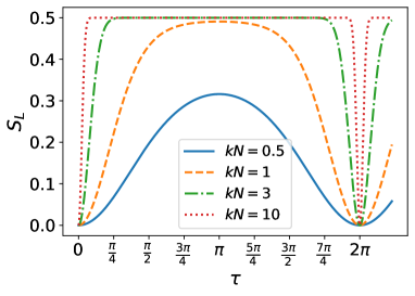
Figure S1: Linear entropy $S_{L}$ as a function of time $\tau$ for various $kN$ values. Entanglement increases with $kN$ and saturates for $kN>1$, with the system disentangling at $\tau=2\pi$ multiples.

In Fig. S1, we plot the linear entropy $S_{L}$ as a function of time $\tau$ for several values of $kN$. As the figure shows, increasing the value of $kN$ leads to increased entanglement, which saturates for values $kN>1$. Interestingly, regardless of the values of $kN$, the system disentangles at multiples of $\tau=2\pi$. Note that the disentanglement point provides the highest value of quantum Fisher information, as opposed to the highly entangled state typically used for quantum enhancement. This is because the inherent parametric nature of the spin-mechanical system dynamically transfers all the information encoded in the field mode to the spin subsystem.

V V. $N$-spins quantum Fisher information: reduced density matrix of the spin subsystem

As discussed in the main text, we can investigate the precision limits when there is partial accessibility to the system. Specifically, to determine the sensing capability of the spin subsystem, we compute its reduced density matrix as follows:

$$\rho_{\mathrm{spin}}=\rho_{\mathrm{spin}}(g)=\text{Tr}_{\text{field}}\left[(\left|\psi(\tau)\right\rangle\left\langle\psi(\tau)\right|)_{\mathrm{sm}}^{(\text{GHZ})}\right],$$ (S41)

where the state $\left|\psi(\tau)\right\rangle_{\mathrm{sm}}^{(\text{GHZ})}$ has been derived in Eq. (S30). To compute the quantum Fisher information for density matrices, we use:

$$\mathcal{Q}_{\mathrm{sm}}=2\sum_{n,m}\frac{|\langle\lambda_{m}|\partial_{g}\rho_{\mathrm{spin}}|\lambda_{n}\rangle|^{2}}{\lambda_{n}+\lambda_{m}},\hskip 14.22636pt\lambda_{n}+\lambda_{m}\neq 0,$$ (S42)

where $\rho_{\mathrm{spin}}=\sum_{i}\lambda_{i}|\lambda_{i}\rangle\langle\lambda_{i}|$ is represented in its spectral decomposition, with $\lambda_{i}$ and $|\lambda_{i}\rangle$ being the $i$th eigenvalue and eigenvector of $\rho_{\mathrm{spin}}$, respectively. Hence, let us gather the necessary ingredients to evaluate the quantum Fisher information. The reduced density matrix is:

$$\rho_{\mathrm{spin}}=\left(\begin{array}[]{cc}\frac{1}{2}&\frac{1}{2}e^{k^{2}L^{2}(\cos\tau-1)}e^{2ikN(\alpha\sin\tau+g\cos\xi)(\sin\tau-\tau)}\\ \frac{1}{2}e^{k^{2}L^{2}(\cos\tau-1)}e^{-2ikN(\alpha\sin\tau+g\cos\xi)(\sin\tau-\tau)}&\frac{1}{2}\\ \end{array}\right),$$ (S43)

with eigenvalues:

$$\lambda_{1} = \frac{1}{2}\left(1-e^{k^{2}N^{2}(\cos\tau-1}\right),$$ (S44)

$$\lambda_{2} = \frac{1}{2}\left(1+e^{k^{2}N^{2}(\cos\tau-1}\right),$$ (S45)

and eigenvectors:

$$|\lambda_{1}\rangle = \frac{1}{\sqrt{2}}\left(-e^{2ikN(\alpha\sin\tau+g\cos\xi(\sin\tau-\tau))}\left|\frac{N}{2},\frac{N}{2}\right\rangle+\left|\frac{N}{2},-\frac{N}{2}\right\rangle\right),$$ (S46)

$$|\lambda_{2}\rangle = \frac{1}{\sqrt{2}}\left(e^{2ikN(\alpha\sin\tau+g\cos\xi(\sin\tau-\tau))}\left|\frac{N}{2},\frac{N}{2}\right\rangle+\left|\frac{N}{2},-\frac{N}{2}\right\rangle\right).$$ (S47)

From which one can easily derive the expression shown in the main text; see Eq. (12):

$$\mathcal{Q}_{\mathrm{sm}}=2\sum_{n,m}\frac{|\langle\lambda_{m}|\partial_{g}\rho_{\mathrm{spin}}|\lambda_{n}\rangle|^{2}}{\lambda_{n}+\lambda_{m}}=4e^{2k^{2}N^{2}(\cos\tau{-}1)}k^{2}N^{2}(\tau{-}\sin\tau)^{2}.$$ (S48)

VI VI. Quantum Fisher information in the vicinity of $\tau=2\pi$

A common challenge in achieving the Heisenberg limit of precision is its fragility to particle losses (e.g., losing just a single particle in N00N states Kacprowicz et al. (2010) ($|N00N\rangle\sim|N,0\rangle+|0,N\rangle$) can eliminate the ultimate sensing precision) and the necessity of fine-tuning the parameter(s) that enable this limit. The latter is particularly well-known in physical systems undergoing a quantum phase transition. In fact, it can be rigorously shown that at the critical point the quantum Fisher information scales as Rams et al. (2018): $\mathcal{Q}\sim N^{\frac{2}{d\tilde{\nu}}}$, where $N$ is the number of particles, $d$ is the spatial dimension of the probe, and $\tilde{\nu}$ is the critical exponent related to the correlation length. Conversely, near the critical point, the quantum Fisher information scales as: $\mathcal{Q}\sim N|\Lambda-\Lambda_{c}|^{d\tilde{\nu}-2}$, where $\Lambda_{c}$ is the critical point and $\Lambda$ is the parameter driving the quantum phase transition. For the paradigmatic one-dimensional Ising model in a transverse field, $d=\tilde{\nu}=1$, and one recast the quadratic scaling with respect to the number of particles—the Heisenberg limit.

In the main text, we have analytically proven that the quantum Fisher information for the entire spin-mechanical system scales quadratically with the number of spins, achieving the Heisenberg limit of precision, see Eq. (10). However, when the mechanical degrees of freedom are traced out, the quantum Fisher information of the spin subsystem becomes:

$$\mathcal{Q}_{\mathrm{spin}}{=}4e^{2k^{2}N^{2}(\cos\tau{-}1)}k^{2}N^{2}(\tau{-}\sin\tau)^{2}.$$ (S49)

In the above equation, the Heisenberg limit for gravimetry is maintained at times $\tau$ that are multiples of $2\pi$. However, at other times $\tau$ (not multiples of $2\pi$), the quantum Fisher information of the reduced density matrix of the spins exponentially decreases due to the factor $e^{2k^{2}N^{2}(\cos\tau-1)}$. Therefore, it is important to assess the gravimetry precision limits achieved by the spin subsystem in the vicinity of $\tau=2\pi$. In Figs. S2, we evaluate Eq. (S49) (blue dots) as a function of $N$ for different values of $k$ and times in the vicinity of $\tau=2\pi$. As shown in the figures, the Heisenberg limit is rapidly lost near $\tau=2\pi$. Although a super-linear scaling is observed in Fig. S2(a), this behavior quickly diminishes when either the coupling constant $k$ increases or the time $\tau$ deviates from $2\pi$. This is clearly illustrated in Fig. S2(d), where for $k=0.5$ and $\tau=0.95\times 2\pi$, the term $e^{2k^{2}N^{2}(\cos\tau-1)}$ in Eq. (S49) becomes dominant. Hence, for $N>10$, the curve vanishes very quickly. The analytical form of Eq. (S49) fully supports all the above description.

Figure S2: Quantum Fisher information for the reduced density matrix of the spin subsystem. (Blue dots) The system evolves from the initial state $|\psi(0)\rangle=|\mathrm{GHZ}\rangle|\alpha\rangle$; (Green triangles) The system evolves from the initial state $|\psi(0)\rangle=|\mathrm{CSS}\rangle|\alpha\rangle$. We consider $\alpha=0$, two values for $k$ (0.1 and 0.5), and two values in the vicinity of $\tau=2\pi$, specifically $\tau=0.99\times 2\pi$ and $\tau=0.95\times 2\pi$. Even in the absence of the Heisenberg limit, the $\mathrm{GHZ}$ scenario significantly outperforms the $\mathrm{CSS}$ scenario in several instances.

Nonetheless, it is important not to confuse losing the Heisenberg limit of precision with losing any quantum enhancement in precision. Even if the Heisenberg limit is not achieved, multiplicative factors $a$ in the scaling of the quantum Fisher information, $\mathcal{Q}\sim aN^{b}$, can still result in higher values compared to classical probes of which $\mathcal{Q}\sim cN$, where $c$ is a real coefficient. Consequently, the quantum probe can still offer better precision than classical probes. To address this issue, we evaluate the quantum Fisher information for a purely classical spin state, where all spins are in a product of individual separable states, defined as follows Pezzè et al. (2018):

$$|\mathrm{CSS}\rangle=\bigotimes_{j=1}^{N}\frac{1}{\sqrt{2}}(|0\rangle+|1\rangle)_{j}=\sum_{m=-\frac{N}{2}}^{\frac{N}{2}}\binom{N}{\frac{N}{2}+m}\left(\frac{1}{\sqrt{2}}\right)^{\frac{N}{2}+m}\left(\frac{1}{\sqrt{2}}\right)^{\frac{N}{2}-m}\left|\frac{N}{2},m\right\rangle.$$ (S50)

The state described above is known as a coherent spin state (CSS) Pezzè et al. (2018). In this state, all spins are in separable states and are collectively aligned in the same direction, which we assume to be the $z-$direction. We now numerically simulate the quantum Fisher information for the reduced density matrix of the spins as the system evolves from the initial state $|\psi(0)\rangle_{\mathrm{CSS}}=|\mathrm{CSS}\rangle|\alpha\rangle$. In Figs. S2, we illustrate such quantum Fisher information for the CSS spin subsystem (green triangles) as a function of the number of spins $N$ for different values of the coupling parameter $k$ and evolution times $\tau$. As the figure shows, in most cases, the quantum Fisher information for the GHZ spin subsystem significantly outperforms that of the CSS spin subsystem. This remains true even in the absence of the Heisenberg limit of precision. However, for very large $N\gg 1$, the exponential factor $e^{2k^{2}N^{2}(\cos\tau-1)}$ dominates, causing the quantum Fisher information for the GHZ spin subsystem to eventually vanish. Only when the prefactor $e^{2k^{2}N^{2}(\cos\tau-1)}$ becomes larger—by increasing $k$ and choosing $\tau$ far from $\tau=2\pi$—does the quantum Fisher information for the CSS spin subsystem perform better than in the GHZ case. Note that, in Fig. S2(d), the quantum Fisher information for the CSS spin subsystem is observed to be sublinear (this is because, in most cases, accessing only the spin subsystem results in a loss of information about the gravitational acceleration). To demonstrate that the quantum Fisher information for the entire spin-mechanical system, which evolves from the initial state $|\psi(0)\rangle=|\mathrm{CSS}\rangle$, is linear for CSS, one can directly obtain its analytical solution as follows:

$$\mathcal{Q}_{\mathrm{spin}}^{\mathrm{(CSS)}}(\tau)=8-8\cos\tau+\frac{2k^{2}N\Gamma\left(\frac{1+N}{2}\right)}{\sqrt{\pi}}\left[\frac{2+3N}{\Gamma\left(2+\frac{N}{2}\right)}+\frac{(-2+N)}{\Gamma\left(\frac{6+N}{2}\right)}N\,{}_{2}F_{1}\left(1,2-\frac{N}{2};\frac{6+N}{2};-1\right)\right](\tau-\sin\tau)^{2},$$ (S51)

where ${}_{2}F_{1}(a,b;c;z)$ is the hypergeometric function. In the particular case of $\tau=2\pi$, the quantum Fisher information function reduces to:

$$\mathcal{Q}_{\mathrm{spin}}^{\mathrm{(CSS)}}(\tau=2\pi)=8\pi^{3/2}k^{2}N\Gamma\left(\frac{1+N}{2}\right)\left[\frac{2+3N}{\Gamma\left(2+\frac{N}{2}\right)}+\frac{(-2+N)N{}_{2}F_{1}\left(1,2-\frac{N}{2};\frac{6+N}{2};-1\right)}{\Gamma\left(\frac{6-N}{2}\right)}\right].$$ (S52)

VII VII. Classical Fisher information for the spin subsystem: analytical form

Here, we present the analytical form of the classical Fisher information function for the reduced density matrix of the spin subsystem $\mathcal{F}_{\mathrm{spin}}$. To achieve this, we directly evaluate the conditional probability distribution $p(\Upsilon(\Theta,\Phi)|g)$ as follows:

$$p(\Upsilon(\Theta{,}\Phi)|g) = \left\langle\psi(\tau)\right|\hat{\Pi}_{\Upsilon}\left|\psi(\tau)\right\rangle$$ (S53)

$$= \frac{1}{2}\Big{(}1+\exp\left[k^{2}N^{2}(-1+\cos\tau)\right]\sin\theta\cos\left[\phi{+}2gkN\tau\cos\xi{-}2kN[\alpha+g\cos\xi]\sin\tau\right]\Big{)}.$$ (S54)

With the above expression, it is straightforward to evaluate the classical Fisher information as follows:

$$\mathcal{F}_{\mathrm{spin}}=-\frac{4e^{2k^{2}N^{2}(-1+\cos\tau)}k^{2}N^{2}\cos^{2}\xi(t-\sin\tau)^{2}\sin^{2}\theta\sin^{2}\left(\phi+2gkN\tau\cos\xi-2kN(\alpha+g\cos\xi)\sin\tau\right)}{-1+e^{2k^{2}N^{2}(-1+\cos\tau)}\sin^{2}\theta\cos^{2}\left(\phi+2gkN\tau\cos\xi-2kN(\alpha+g\cos\xi)\sin\tau\right)}.$$ (S55)

As the above expression shows, the comparison between $\mathcal{F}_{\mathrm{spin}}$ and $\mathcal{Q}_{\mathrm{spin}}$ must be made with respect to the product $kN$. This is because both the quantum and classical Fisher information functions inherently depend on the term $kN$. Therefore, the results will be identical for any combination of $k$ and $N$ that yields the same product $kN$. It is the product $kN$ that is significant, not the individual values of $k$ or $N$ alone.

VIII VIII. Homodyne, heterodyne, and photocounting measurements

Throughout the main text, we assume we cannot access the mechanical mode. However, in cases where we do have access, we are typically limited to measurements using homodyne, heterodyne, and photocounting techniques. From an experimental perspective, we consider uncorrelated field and spin measurements.

For the homodyne scheme, the joint Fisher information is:

$$\mathcal{F}_{\mathrm{sm}}{=}\max_{\{\Theta,\Phi\}}\left[\int_{-\infty}^{\infty}\frac{\left(\partial_{g}p(\Upsilon(\Theta{,}\Phi),x|g)\right]^{2}}{p(\Upsilon(\Theta{,}\Phi),x|g)[1{-}p(\Upsilon(\Theta{,}\Phi),x|g)]}dx\right],$$ (S56)

where $p(\Upsilon(\Theta{,}\Phi),x|g){=}\left\langle\psi(\tau)\right|(\hat{\Pi}_{\Upsilon}{\otimes}\left|x_{\lambda}\right\rangle\langle x_{\lambda}|)\left|\psi(\tau)\right\rangle$ is the conditional probability associated to POVMs $\hat{\Pi}_{\Upsilon}{\otimes}\left|x_{\lambda}\right\rangle\langle x_{\lambda}|$ and $\left|x_{\lambda}\right\rangle$ is the eigenstate of the rotated quadrature $\sqrt{2}\hat{x}_{\lambda}{=}\hat{a}e^{-i\lambda}{+}\hat{a}^{\dagger}e^{i\lambda}$. In Fock basis representation it reads $\langle n|x_{\lambda}\rangle{=}\pi^{-1/4}2^{-n/2}(n!)^{-1/2}\mathrm{exp}[-x_{\lambda}^{2}/2]\mathcal{H}_{n}(x_{\lambda})\mathrm{exp}[in\lambda]$; where $n$ is the Fock number state and $\mathcal{H}_{n}(x_{\lambda})$ are the Hermite polynomials of order $n$. In Fig. S3, we compare the CFI from both measuring the spin subsystem ($\mathcal{F}_{\mathrm{spin}}$) and the spin-mechanical system ($\mathcal{F}_{\mathrm{sm}}$) with the ultimate gravimetry precision given by the QFI of the entire system ($\mathcal{Q}_{\mathrm{sm}}$) as a function of time $\tau$ and different values of $kN$. As seen from Figs. S3(a)-(b), for $kN{\lesssim}0.1$, most of the information content with respect to $g$ is encoded in the mechanical subsystem, which can be fairly extracted using homodyne detection. In Fig. S3(c), for values $kN{\gtrsim}1$, measuring the field via homodyne detection results in poor performance across all times. Measuring only the spin subsystem yields excellent performance at and around $\tau{\rightarrow}2\pi$.

Figure S3: All panels depict the classical Fisher information obtained solely from measurements on the spin subsystem $\mathcal{F}_{\mathrm{spin}}$ and the ultimate gravimetry precision quantified by the spin-mechanical quantum Fisher information $\mathcal{Q}_{\mathrm{sm}}$ as a function of time $\tau$ for different values of $kN$. Panels (a)-(c) include the classical Fisher information from uncorrelated measurements on the spin and the field via homodyne detection $\mathcal{F}_{\mathrm{sm}}$; panels (d)-(f) consider the classical Fisher information obtained from uncorrelated heterodyne measurements and spin measurements $\mathcal{F}_{\mathrm{sm}}^{\mathrm{hete.}}$; and panels (g)-(i) show the classical Fisher information obtained from uncorrelated photocounting measurements and spin measurements $\mathcal{F}_{\mathrm{sm}}^{\mathrm{phot.}}$.

For heterodyne detection, the conditional probability needed to evaluate the classical Fisher information is:

$$p(\Upsilon(\Theta{,}\Phi),\zeta|g)=\frac{1}{\pi}\left\langle\psi(\tau)\right|(\hat{\Pi}_{\Upsilon}\otimes\left|\zeta\right\rangle\left\langle\zeta\right|)|\psi(\tau)\rangle,$$ (S57)

where $\left|\zeta\right\rangle$ is a coherent state with $\zeta\in\mathbb{C}$. Therefore, the classical Fisher information is computed as:

$$\mathcal{F}_{\mathrm{spin}}^{\mathrm{hete.}}=\max_{\{\Theta,\Phi\}}\left[\int d^{2}\zeta\frac{\left(\partial_{g}p(\Upsilon(\Theta{,}\Phi),\zeta|g)\right)^{2}}{p(\Upsilon(\Theta{,}\Phi),\zeta|g)[1{-}p(\Upsilon(\Theta{,}\Phi),\zeta|g)]}\right].$$ (S58)

Similarly, for the photocounting scheme, the conditional probability is:

$$p(\Upsilon(\Theta{,}\Phi),n|g)=\left\langle\psi(\tau)\right|(\hat{\Pi}_{\Upsilon}\otimes\left|n\right\rangle\left\langle n\right|)|\psi(\tau)\rangle,$$ (S59)

where $\left|n\right\rangle$ is a Fock number state. Hence:

$$\mathcal{F}_{\mathrm{spin}}^{\mathrm{phot.}}=\max_{\{\Theta,\Phi\}}\left[\sum_{n=0}^{\infty}\frac{\left(\partial_{g}p(\Upsilon(\Theta{,}\Phi),n|g)\right)^{2}}{p(\Upsilon(\Theta{,}\Phi),n|g)[1{-}p(\Upsilon(\Theta{,}\Phi),n|g)]}\right].$$ (S60)

In Figs. S3(d)-(f), we plot the classical Fisher information obtained from uncorrelated heterodyne measurements and spin measurements $\mathcal{F}_{\mathrm{sm}}^{\mathrm{hete.}}$ as a function of time $\tau$ for several values of $kN$. In Figs. S3(g)-(i), we plot the classical Fisher information obtained from uncorrelated photocounting measurements and spin measurements $\mathcal{F}_{\mathrm{sm}}^{\mathrm{phot.}}$ as a function of time $\tau$ and different $kN$. The figures show that the homodyne measurement scheme outperforms the other cases.

IX IX. Predicted sensitivity

To quantify the sensitivity of our scheme, we can evaluate $\Delta\bar{g}$ as follows Armata et al. (2017):

$$\Delta\bar{g}=\frac{1}{\sqrt{\nu\mathcal{Q}_{\mathrm{sm}}}},$$ (S61)

Here, $\nu$ represents the number of measurement trials, $\mathcal{Q}_{\mathrm{sm}}$ denotes the quantum Fisher information of the entire spin-mechanical system, and $\bar{g}$ is the magnitude of gravitational acceleration in the International System of Units (SI), with $[\bar{g}]=\frac{m}{s^{2}}$. For reference, see the Hamiltonian in Eq. (3). Throughout our work, we have rescaled $\bar{g}$, making it straightforward to revert to SI units by applying the chain rule: $\frac{\partial}{\partial\bar{g}}=\frac{\partial}{\partial g}\frac{\partial g}{\partial\bar{g}}$. Therefore,

$$\mathcal{Q}_{\mathrm{sm}}{=}4\left(\frac{\partial g}{\partial\bar{g}}\right)^{2}\mathbb{R}\text{e}\left[\langle\partial_{g}\psi(\tau)|\partial_{g}\psi(\tau)\rangle{-}|\langle\partial_{g}\psi(\tau)|\psi(\tau)\rangle|^{2}\right].$$ (S62)

We aim to quantify the predicted sensitivity $\Delta\bar{g}$ for a vertically oriented spin-mechanical gravimeter $\xi=0$, specifically when $\nu=10^{3}$, $\tau=2\pi$ and the spin-coupling constant $k$ is of the order of unity, with $k=1$. Under these conditions, and recalling that $\hbar g{:=}\bar{g}\sqrt{M\hbar/(2\omega^{3})}\cos\xi$, the sensitivity in SI units simplifies to:

$$\Delta\bar{g}\approx 10^{-19}\frac{1}{N}\sqrt{\frac{\omega^{3}}{M}}.$$ (S63)

Here, $N$ is the number of spin particles, $\omega$ is the angular frequency, and $M$ is the mass of the mechanical harmonic oscillator. Eq. (S63) presents the predicted gravimetry sensitivity for this work. Since $\omega$ and $M$ vary depending on the physical device, in Figs. S4, we plot the predicted sensitivity $\Delta\bar{g}$ on a $\mathrm{log}_{10}$ scale as a function of $\omega$ and $M$ in SI units for different values of $N$. As highlighted by an arrow in the figure, a very moderate set of parameters could achieve predicted sensitivities of $\Delta\bar{g}\sim 10^{-9}m/s^{2}$. This sensitivity could be further improved by adjusting the mass and frequency. Experimentally, the sensitivity $\Delta\bar{g}$ typically ranges from $10^{-5}m/s^{2}$ to $10^{-10}m/s^{2}$, while theoretical predictions span from $10^{-7}m/s^{2}$ to $10^{-15}m/s^{2}$, see comparison table in Ref. Qvarfort et al. (2018). Thus, even the simplest triplet scenario with $N=2$ in this work could potentially compete with other proposals, without relying on free-fall-based methodologies or the need for ground-state cooling.

Figure S4: Predicted sensitivity $\Delta\bar{g}$ plotted on a $\mathrm{log}_{10}$ scale as a function of $\omega$ and $M$ in SI units for various values of $N$. The arrow highlights that a moderate set of parameters can achieve predicted sensitivities of $\Delta\bar{g}\sim 10^{-9}$ m$/$s².

References

- Ciufolini et al. (2016) Ignazio Ciufolini, Antonio Paolozzi, Erricos C. Pavlis, Rolf Koenig, John Ries, Vahe Gurzadyan, Richard Matzner, Roger Penrose, Giampiero Sindoni, Claudio Paris, Harutyun Khachatryan, and Sergey Mirzoyan, “A test of general relativity using the lares and lageos satellites and a grace earth gravity model,” The European Physical Journal C 76, 120 (2016).
- Asenbaum et al. (2020) Peter Asenbaum, Chris Overstreet, Minjeong Kim, Joseph Curti, and Mark A Kasevich, “Atom-interferometric test of the equivalence principle at the 10-12 level,” Physical Review Letters 125, 191101 (2020).
- Biswas et al. (2012) Tirthabir Biswas, Erik Gerwick, Tomi Koivisto, and Anupam Mazumdar, “Towards singularity-and ghost-free theories of gravity,” Physical review letters 108, 031101 (2012).
- Van Camp et al. (2017) Michel Van Camp, Olivier de Viron, Arnaud Watlet, Bruno Meurers, Olivier Francis, and Corentin Caudron, “Geophysics from terrestrial time-variable gravity measurements,” Reviews of Geophysics 55, 938–992 (2017).
- Pearson-Grant et al. (2018) SC Pearson-Grant, P Franz, and J Clearwater, “Gravity measurements as a calibration tool for geothermal reservoir modelling,” Geothermics 73, 146–157 (2018).
- Carbone et al. (2017) Daniele Carbone, Michael P Poland, Michel Diament, and Filippo Greco, “The added value of time-variable microgravimetry to the understanding of how volcanoes work,” Earth-Science Reviews 169, 146–179 (2017).
- van Dam et al. (2017) Tonie van Dam, Olivier Francis, J Wahr, Shfaqat Abbas Khan, M Bevis, and Michiel R van den Broeke, “Using gps and absolute gravity observations to separate the effects of present-day and pleistocene ice-mass changes in south east greenland,” Earth and Planetary Science Letters 459, 127–135 (2017).
- Romaides et al. (2001) Anestis J Romaides, James C Battis, Roger W Sands, Alan Zorn, Donald O Benson Jr, and Daniel J DiFrancesco, “A comparison of gravimetric techniques for measuring subsurface void signals,” Journal of Physics D: Applied Physics 34, 433 (2001).
- Iess et al. (2018) Luciano Iess, WM Folkner, D Durante, M Parisi, Y Kaspi, E Galanti, Tristan Guillot, WB Hubbard, DJ Stevenson, JD Anderson, et al., “Measurement of jupiter’s asymmetric gravity field,” Nature 555, 220–222 (2018).
- Flechtner et al. (2021) Frank Flechtner, Christoph Reigber, Reiner Rummel, and Georges Balmino, “Satellite gravimetry: A review of its realization,” Surveys in Geophysics 42, 1029–1074 (2021).
- Pail (2014) Roland Pail, “Champ-, grace-, goce-satellite projects,” in Encyclopedia of Geodesy, edited by Erik Grafarend (Springer International Publishing, Cham, 2014) pp. 1–11.
- Ebbing et al. (2018) Jörg Ebbing, Peter Haas, Fausto Ferraccioli, Folker Pappa, Wolfgang Szwillus, and Johannes Bouman, “Earth tectonics as seen by goce - enhanced satellite gravity gradient imaging,” Scientific Reports 8, 16356 (2018).
- Visser (1999) P.N.A.M. Visser, “Gravity field determination with goce and grace,” Advances in Space Research 23, 771–776 (1999).
- Rademacher et al. (2020) Markus Rademacher, James Millen, and Ying Lia Li, “Quantum sensing with nanoparticles for gravimetry: when bigger is better,” Advanced Optical Technologies 9, 227–239 (2020).
- Marson and Faller (1986) I Marson and J E Faller, “g-the acceleration of gravity: its measurement and its importance,” Journal of Physics E: Scientific Instruments 19, 22 (1986).
- Zhong et al. (2022) Jiaqi Zhong, Biao Tang, Xi Chen, and Lin Zhou, “Quantum gravimetry going toward real applications,” Innovation (Camb) 3, 100230 (2022).
- Treutlein et al. (2014) Philipp Treutlein, Claudiu Genes, Klemens Hammerer, Martino Poggio, and Peter Rabl, “Hybrid mechanical systems,” in Cavity Optomechanics (Springer Berlin Heidelberg, 2014) p. 327–351.
- Janvier et al. (2022) Camille Janvier, Vincent Ménoret, Bruno Desruelle, Sébastien Merlet, Arnaud Landragin, and Franck Pereira dos Santos, “Compact differential gravimeter at the quantum projection-noise limit,” Phys. Rev. A 105, 022801 (2022).
- Stray et al. (2022) Ben Stray, Andrew Lamb, Aisha Kaushik, Jamie Vovrosh, Anthony Rodgers, Jonathan Winch, Farzad Hayati, Daniel Boddice, Artur Stabrawa, Alexander Niggebaum, Mehdi Langlois, Yu-Hung Lien, Samuel Lellouch, Sanaz Roshanmanesh, Kevin Ridley, Geoffrey de Villiers, Gareth Brown, Trevor Cross, George Tuckwell, Asaad Faramarzi, Nicole Metje, Kai Bongs, and Michael Holynski, “Quantum sensing for gravity cartography,” Nature 602, 590–594 (2022).
- Freier et al. (2016) C Freier, M Hauth, V Schkolnik, B Leykauf, M Schilling, H Wziontek, H-G Scherneck, J Müller, and A Peters, “Mobile quantum gravity sensor with unprecedented stability,” Journal of Physics: Conference Series 723, 012050 (2016).
- Peters et al. (2001) Achim Peters, Keng Yeow Chung, and Steven Chu, “High-precision gravity measurements using atom interferometry,” Metrologia 38, 25 (2001).
- Mcguirk et al. (2002) Jeffrey Michael Mcguirk, GT Foster, JB Fixler, MJ Snadden, and MA Kasevich, “Sensitive absolute-gravity gradiometry using atom interferometry,” Physical Review A 65, 033608 (2002).
- Bidel et al. (2013) Yannick Bidel, Olivier Carraz, Renée Charrière, Malo Cadoret, Nassim Zahzam, and Alexandre Bresson, “Compact cold atom gravimeter for field applications,” Applied Physics Letters 102, 144107 (2013).
- Kritsotakis et al. (2018) Michail Kritsotakis, Stuart S. Szigeti, Jacob A. Dunningham, and Simon A. Haine, “Optimal matter-wave gravimetry,” Phys. Rev. A 98, 023629 (2018).
- Hu et al. (2013) Zhong-Kun Hu, Bu-Liang Sun, Xiao-Chun Duan, Min-Kang Zhou, Le-Le Chen, Su Zhan, Qiao-Zhen Zhang, and Jun Luo, “Demonstration of an ultrahigh-sensitivity atom-interferometry absolute gravimeter,” Phys. Rev. A 88, 043610 (2013).
- Monteiro et al. (2017) Fernando Monteiro, Sumita Ghosh, Adam Getzels Fine, and David C. Moore, “Optical levitation of 10-ng spheres with nano- acceleration sensitivity,” Phys. Rev. A 96, 063841 (2017).
- Monteiro et al. (2020) Fernando Monteiro, Wenqiang Li, Gadi Afek, Chang-ling Li, Michael Mossman, and David C. Moore, “Force and acceleration sensing with optically levitated nanogram masses at microkelvin temperatures,” Phys. Rev. A 101, 053835 (2020).
- Armata et al. (2017) F. Armata, L. Latmiral, A. D. K. Plato, and M. S. Kim, “Quantum limits to gravity estimation with optomechanics,” Phys. Rev. A 96, 043824 (2017).
- Feng et al. (2020) Ling-Juan Feng, Gong-Wei Lin, Yue-Ping Niu, and Shang-Qing Gong, “Enhancement of gravity estimation in modulated optomechanics,” Optics Communications 460, 125217 (2020).
- Xiao et al. (2020) Xiao Xiao, Hongbin Liang, and Xiaoguang Wang, “Optimal estimation of gravitation with kerr nonlinearity in an optomechanical system,” Quantum Information Processing 19, 410 (2020).
- Qvarfort et al. (2021) Sofia Qvarfort, A. Douglas K. Plato, David Edward Bruschi, Fabienne Schneiter, Daniel Braun, Alessio Serafini, and Dennis Rätzel, “Optimal estimation of time-dependent gravitational fields with quantum optomechanical systems,” Phys. Rev. Res. 3, 013159 (2021).
- Qvarfort et al. (2018) Sofia Qvarfort, Alessio Serafini, P. F. Barker, and Sougato Bose, “Gravimetry through non-linear optomechanics,” Nature Communications 9, 3690 (2018).
- Johnsson et al. (2016) Mattias T. Johnsson, Gavin K. Brennen, and Jason Twamley, “Macroscopic superpositions and gravimetry with quantum magnetomechanics,” Scientific Reports 6, 37495 (2016).
- Geraci and Goldman (2015) Andrew Geraci and Hart Goldman, “Sensing short range forces with a nanosphere matter-wave interferometer,” Phys. Rev. D 92, 062002 (2015).
- Abend et al. (2016) S. Abend, M. Gebbe, M. Gersemann, H. Ahlers, H. Müntinga, E. Giese, N. Gaaloul, C. Schubert, C. Lämmerzahl, W. Ertmer, W. P. Schleich, and E. M. Rasel, “Atom-chip fountain gravimeter,” Phys. Rev. Lett. 117, 203003 (2016).
- Ke et al. (2018) Yongguan Ke, Jiahao Huang, Min Zhuang, Bo Lu, and Chaohong Lee, “Compact gravimeter with an ensemble of ultracold atoms in spin-dependent optical lattices,” Phys. Rev. A 98, 053826 (2018).
- Phillips et al. (2022) Alexander M. Phillips, Michael J. Wright, Isabelle Riou, Stephen Maddox, Simon Maskell, and Jason F. Ralph, “Position fixing with cold atom gravity gradiometers,” AVS Quantum Science 4 (2022).
- Szigeti et al. (2020) Stuart S. Szigeti, Samuel P. Nolan, John D. Close, and Simon A. Haine, “High-precision quantum-enhanced gravimetry with a bose-einstein condensate,” Phys. Rev. Lett. 125, 100402 (2020).
- Gietka et al. (2019) Karol Gietka, Farokh Mivehvar, and Helmut Ritsch, “Supersolid-based gravimeter in a ring cavity,” Phys. Rev. Lett. 122, 190801 (2019).
- Middlemiss et al. (2016) R. P. Middlemiss, A. Samarelli, D. J. Paul, J. Hough, S. Rowan, and G. D. Hammond, “Measurement of the earth tides with a mems gravimeter,” Nature 531, 614–617 (2016).
- Prasad et al. (2022) Abhinav Prasad, Richard P. Middlemiss, Andreas Noack, Kristian Anastasiou, Steven G. Bramsiepe, Karl Toland, Phoebe R. Utting, Douglas J. Paul, and Giles D. Hammond, “A 19 day earth tide measurement with a mems gravimeter,” Scientific Reports 12, 13091 (2022).
- Mustafazade et al. (2020) Arif Mustafazade, Milind Pandit, Chun Zhao, Guillermo Sobreviela, Zhijun Du, Philipp Steinmann, Xudong Zou, Roger T. Howe, and Ashwin A. Seshia, “A vibrating beam mems accelerometer for gravity and seismic measurements,” Scientific Reports 10, 10415 (2020).
- Tang et al. (2019) Shihao Tang, Huafeng Liu, Shitao Yan, Xiaochao Xu, Wenjie Wu, Ji Fan, Jinquan Liu, Chenyuan Hu, and Liangcheng Tu, “A high-sensitivity mems gravimeter with a large dynamic range,” Microsystems & Nanoengineering 5, 45 (2019).
- Krishnamoorthy et al. (2008) U. Krishnamoorthy, R.H. Olsson, G.R. Bogart, M.S. Baker, D.W. Carr, T.P. Swiler, and P.J. Clews, “In-plane mems-based nano-g accelerometer with sub-wavelength optical resonant sensor,” Sensors and Actuators A: Physical 145-146, 283–290 (2008).
- Liu et al. (2019) Huafeng Liu, W.T. Pike, Constantinos Charalambous, and Alexander E. Stott, “Passive method for reducing temperature sensitivity of a microelectromechanical seismic accelerometer for marsquake monitoring below 1 nano-,” Phys. Rev. Appl. 12, 064057 (2019).
- Merlet et al. (2021) Sébastien Merlet, Pierre Gillot, Bing Cheng, Romain Karcher, Almazbek Imanaliev, Ludger Timmen, and Franck Pereira dos Santos, “Calibration of a superconducting gravimeter with an absolute atom gravimeter,” Journal of Geodesy 95, 62 (2021).
- Scala et al. (2013) M. Scala, M. S. Kim, G. W. Morley, P. F. Barker, and S. Bose, “Matter-wave interferometry of a levitated thermal nano-oscillator induced and probed by a spin,” Phys. Rev. Lett. 111, 180403 (2013).
- Wan et al. (2016) C. Wan, M. Scala, G. W. Morley, ATM. A. Rahman, H. Ulbricht, J. Bateman, P. F. Barker, S. Bose, and M. S. Kim, “Free nano-object ramsey interferometry for large quantum superpositions,” Phys. Rev. Lett. 117, 143003 (2016).
- Chen and Yin (2018) Xing-Yan Chen and Zhang-Qi Yin, “High-precision gravimeter based on a nano-mechanical resonator hybrid with an electron spin,” Opt. Express 26, 31577–31588 (2018).
- Hebestreit et al. (2018) Erik Hebestreit, Martin Frimmer, René Reimann, and Lukas Novotny, “Sensing static forces with free-falling nanoparticles,” Phys. Rev. Lett. 121, 063602 (2018).
- Wei et al. (2006) L. F. Wei, Yu-xi Liu, and Franco Nori, “Generation and control of greenberger-horne-zeilinger entanglement in superconducting circuits,” Phys. Rev. Lett. 96, 246803 (2006).
- Hendrickx et al. (2021) Nico W. Hendrickx, William I. L. Lawrie, Maximilian Russ, Floor van Riggelen, Sander L. de Snoo, Raymond N. Schouten, Amir Sammak, Giordano Scappucci, and Menno Veldhorst, “A four-qubit germanium quantum processor,” Nature 591, 580–585 (2021).
- Jiang et al. (2009) L. Jiang, J. S. Hodges, J. R. Maze, P. Maurer, J. M. Taylor, D. G. Cory, P. R. Hemmer, R. L. Walsworth, A. Yacoby, A. S. Zibrov, and M. D. Lukin, “Repetitive readout of a single electronic spin via quantum logic with nuclear spin ancillae,” Science 326, 267–272 (2009).
- Shields et al. (2015) B. J. Shields, Q. P. Unterreithmeier, N. P. de Leon, H. Park, and M. D. Lukin, “Efficient readout of a single spin state in diamond via spin-to-charge conversion,” Phys. Rev. Lett. 114, 136402 (2015).
- Rabl et al. (2009) P. Rabl, P. Cappellaro, M. V. Gurudev Dutt, L. Jiang, J. R. Maze, and M. D. Lukin, “Strong magnetic coupling between an electronic spin qubit and a mechanical resonator,” Phys. Rev. B 79, 041302 (2009).
- Tufarelli et al. (2011) Tommaso Tufarelli, M. S. Kim, and Sougato Bose, “Oscillator state reconstruction via tunable qubit coupling in markovian environments,” Phys. Rev. A 83, 062120 (2011).
- Montenegro et al. (2014) Víctor Montenegro, Alessandro Ferraro, and Sougato Bose, “Nonlinearity-induced entanglement stability in a qubit-oscillator system,” Phys. Rev. A 90, 013829 (2014).
- Degen et al. (2017) C. L. Degen, F. Reinhard, and P. Cappellaro, “Quantum sensing,” Rev. Mod. Phys. 89, 035002 (2017).
- Paris (2009) Matteo G. A. Paris, “Quantum estimation for quantum technology,” International Journal of Quantum Information 07, 125–137 (2009).
- Giovannetti et al. (2011) Vittorio Giovannetti, Seth Lloyd, and Lorenzo Maccone, “Advances in quantum metrology,” Nature photonics 5, 222–229 (2011).
- Giovannetti et al. (2004) Vittorio Giovannetti, Seth Lloyd, and Lorenzo Maccone, “Quantum-enhanced measurements: beating the standard quantum limit,” Science 306, 1330–1336 (2004).
- Giovannetti et al. (2006) Vittorio Giovannetti, Seth Lloyd, and Lorenzo Maccone, “Quantum metrology,” Phys. Rev. Lett. 96, 010401 (2006).
- Braun et al. (2018) Daniel Braun, Gerardo Adesso, Fabio Benatti, Roberto Floreanini, Ugo Marzolino, Morgan W. Mitchell, and Stefano Pirandola, “Quantum-enhanced measurements without entanglement,” Rev. Mod. Phys. 90, 035006 (2018).
- Cramér (1999) Harald Cramér, Mathematical methods of statistics, Vol. 26 (Princeton university press, 1999).
- Rao (1992) C. Radhakrishna Rao, “Information and the accuracy attainable in the estimation of statistical parameters,” in Breakthroughs in Statistics: Foundations and Basic Theory, edited by Samuel Kotz and Norman L. Johnson (Springer New York, New York, NY, 1992) pp. 235–247.
- Liu et al. (2016) Jing Liu, Jie Chen, Xiao-Xing Jing, and Xiaoguang Wang, “Quantum fisher information and symmetric logarithmic derivative via anti-commutators,” Journal of Physics A: Mathematical and Theoretical 49, 275302 (2016).
- Sidhu and Kok (2020) Jasminder S. Sidhu and Pieter Kok, “Geometric perspective on quantum parameter estimation,” AVS Quantum Science 2, 014701 (2020).
- Braunstein and Caves (1994) Samuel L. Braunstein and Carlton M. Caves, “Statistical distance and the geometry of quantum states,” Phys. Rev. Lett. 72, 3439–3443 (1994).
- Khosla et al. (2018) K. E. Khosla, M. R. Vanner, N. Ares, and E. A. Laird, “Displacemon electromechanics: How to detect quantum interference in a nanomechanical resonator,” Phys. Rev. X 8, 021052 (2018).
- Rabl et al. (2010) P. Rabl, S. J. Kolkowitz, F. H. L. Koppens, J. G. E. Harris, P. Zoller, and M. D. Lukin, “A quantum spin transducer based on nanoelectromechanical resonator arrays,” Nature Physics 6, 602–608 (2010).
- Rabl (2010) P. Rabl, “Cooling of mechanical motion with a two-level system: The high-temperature regime,” Phys. Rev. B 82, 165320 (2010).
- Braccini et al. (2023) Lorenzo Braccini, Martine Schut, Alessio Serafini, Anupam Mazumdar, and Sougato Bose, “Large spin stern-gerlach interferometry for gravitational entanglement,” (2023), arXiv:2312.05170 [quant-ph] .
- Rao et al. (2016) D. D. Bhaktavatsala Rao, S. Ali Momenzadeh, and Jörg Wrachtrup, “Heralded control of mechanical motion by single spins,” Phys. Rev. Lett. 117, 077203 (2016).
- Montenegro et al. (2017) Víctor Montenegro, Raúl Coto, Vitalie Eremeev, and Miguel Orszag, “Macroscopic nonclassical-state preparation via postselection,” Phys. Rev. A 96, 053851 (2017).
- Tufarelli et al. (2012) Tommaso Tufarelli, Alessandro Ferraro, M. S. Kim, and Sougato Bose, “Reconstructing the quantum state of oscillator networks with a single qubit,” Phys. Rev. A 85, 032334 (2012).
- Montenegro et al. (2018) Víctor Montenegro, Raúl Coto, Vitalie Eremeev, and Miguel Orszag, “Ground-state cooling of a nanomechanical oscillator with spins,” Phys. Rev. A 98, 053837 (2018).
- Yin et al. (2013) Zhang-qi Yin, Tongcang Li, Xiang Zhang, and L. M. Duan, “Large quantum superpositions of a levitated nanodiamond through spin-optomechanical coupling,” Physical Review A 88 (2013).
- Spiller et al. (2006) T P Spiller, Kae Nemoto, Samuel L Braunstein, W J Munro, P van Loock, and G J Milburn, “Quantum computation by communication,” New Journal of Physics 8, 30–30 (2006).
- Kumar and Bhattacharya (2017) Pardeep Kumar and M. Bhattacharya, “Magnetometry via spin-mechanical coupling in levitated optomechanics,” Opt. Express 25, 19568–19582 (2017).
- O’Connell et al. (2010) A. D. O’Connell, M. Hofheinz, M. Ansmann, Radoslaw C. Bialczak, M. Lenander, Erik Lucero, M. Neeley, D. Sank, H. Wang, M. Weides, J. Wenner, John M. Martinis, and A. N. Cleland, “Quantum ground state and single-phonon control of a mechanical resonator,” Nature 464, 697–703 (2010).
- (81) Supplemental Material includes analytical expressions for the quantum Fisher information in the following scenarios: single spin case, two spins scenario, the Greenberger-Horne-Zeilinger case for the entire spin-mechanical system, and the Greenberger-Horne-Zeilinger case specifically for the spin subsystem. Additionally, we illustrate the system’s entanglement and performance when probing the mechanical state using homodyne, heterodyne, and photocounting measurements while optimally measuring the spin, as detailed in the main text.
- Zwierz et al. (2010) Marcin Zwierz, Carlos A. Pérez-Delgado, and Pieter Kok, “General optimality of the heisenberg limit for quantum metrology,” Phys. Rev. Lett. 105, 180402 (2010).
- Fiderer et al. (2019) Lukas J. Fiderer, Julien M. E. Fraïsse, and Daniel Braun, “Maximal quantum fisher information for mixed states,” Phys. Rev. Lett. 123, 250502 (2019).
- Montenegro et al. (2024) Victor Montenegro, Chiranjib Mukhopadhyay, Rozhin Yousefjani, Saubhik Sarkar, Utkarsh Mishra, Matteo G. A. Paris, and Abolfazl Bayat, “Review: Quantum metrology and sensing with many-body systems,” (2024), arXiv:2408.15323 [quant-ph] .
- Montenegro et al. (2022) V. Montenegro, M. G. Genoni, A. Bayat, and M. G. A. Paris, “Probing of nonlinear hybrid optomechanical systems via partial accessibility,” Phys. Rev. Res. 4, 033036 (2022).
- Kacprowicz et al. (2010) M Kacprowicz, R Demkowicz-Dobrzański, W Wasilewski, K Banaszek, and IA Walmsley, “Experimental quantum-enhanced estimation of a lossy phase shift,” Nature Photonics 4, 357–360 (2010).
- Rams et al. (2018) Marek M. Rams, Piotr Sierant, Omyoti Dutta, Paweł Horodecki, and Jakub Zakrzewski, “At the limits of criticality-based quantum metrology: Apparent super-heisenberg scaling revisited,” Phys. Rev. X 8, 021022 (2018).
- Montenegro et al. (2021) Victor Montenegro, Utkarsh Mishra, and Abolfazl Bayat, “Global sensing and its impact for quantum many-body probes with criticality,” Phys. Rev. Lett. 126, 200501 (2021).
- Zhao et al. (2021) Yajuan Zhao, Rui Zhang, Wenlan Chen, Xiang-Bin Wang, and Jiazhong Hu, “Creation of greenberger-horne-zeilinger states with thousands of atoms by entanglement amplification,” npj Quantum Information 7, 24 (2021).
- Wang et al. (2009) Shannon X. Wang, Jaroslaw Labaziewicz, Yufei Ge, Ruth Shewmon, and Isaac L. Chuang, “Individual addressing of ions using magnetic field gradients in a surface-electrode ion trap,” Applied Physics Letters 94, 094103 (2009).
- Monroe et al. (2021) C. Monroe, W. C. Campbell, L.-M. Duan, Z.-X. Gong, A. V. Gorshkov, P. W. Hess, R. Islam, K. Kim, N. M. Linke, G. Pagano, P. Richerme, C. Senko, and N. Y. Yao, “Programmable quantum simulations of spin systems with trapped ions,” Rev. Mod. Phys. 93, 025001 (2021).
- Islam et al. (2011) R. Islam, E. E. Edwards, K. Kim, S. Korenblit, C. Noh, H. Carmichael, G.-D. Lin, L.-M. Duan, C.-C. Joseph Wang, J. K. Freericks, and C. Monroe, “Onset of a quantum phase transition with a trapped ion quantum simulator,” Nature Communications 2, 377 (2011).
- Islam et al. (2013) R. Islam, C. Senko, W. C. Campbell, S. Korenblit, J. Smith, A. Lee, E. E. Edwards, C.-C. J. Wang, J. K. Freericks, and C. Monroe, “Emergence and frustration of magnetism with variable-range interactions in a quantum simulator,” Science 340, 583–587 (2013).
- Richerme et al. (2013) P. Richerme, C. Senko, S. Korenblit, J. Smith, A. Lee, R. Islam, W. C. Campbell, and C. Monroe, “Quantum catalysis of magnetic phase transitions in a quantum simulator,” Phys. Rev. Lett. 111, 100506 (2013).
- Lee et al. (2016) A. C. Lee, J. Smith, P. Richerme, B. Neyenhuis, P. W. Hess, J. Zhang, and C. Monroe, “Engineering large stark shifts for control of individual clock state qubits,” Phys. Rev. A 94, 042308 (2016).
- Mooney et al. (2021) Gary J Mooney, Gregory A L White, Charles D Hill, and Lloyd C L Hollenberg, “Generation and verification of 27-qubit greenberger-horne-zeilinger states in a superconducting quantum computer,” Journal of Physics Communications 5, 095004 (2021).
- Kolkowitz et al. (2012) Shimon Kolkowitz, Ania C. Bleszynski Jayich, Quirin P. Unterreithmeier, Steven D. Bennett, Peter Rabl, J. G. E. Harris, and Mikhail D. Lukin, “Coherent sensing of a mechanical resonator with a single-spin qubit,” Science 335, 1603–1606 (2012).
- Arcizet et al. (2011) O. Arcizet, V. Jacques, A. Siria, P. Poncharal, P. Vincent, and S. Seidelin, “A single nitrogen-vacancy defect coupled to a nanomechanical oscillator,” Nature Physics 7, 879–883 (2011).
- LaHaye et al. (2009) M. D. LaHaye, J. Suh, P. M. Echternach, K. C. Schwab, and M. L. Roukes, “Nanomechanical measurements of a superconducting qubit,” Nature 459, 960–964 (2009).
- Martinetz et al. (2020) Lukas Martinetz, Klaus Hornberger, James Millen, M. S. Kim, and Benjamin A. Stickler, “Quantum electromechanics with levitated nanoparticles,” npj Quantum Information 6, 101 (2020).
- Pirkkalainen et al. (2013) J.-M. Pirkkalainen, S. U. Cho, Jian Li, G. S. Paraoanu, P. J. Hakonen, and M. A. Sillanpää, “Hybrid circuit cavity quantum electrodynamics with a micromechanical resonator,” Nature 494, 211–215 (2013).
- Aporvari and Vitali (2021) Ahmad Shafiei Aporvari and David Vitali, “Strong coupling optomechanics mediated by a qubit in the dispersive regime,” Entropy 23, 966 (2021).
- Pirkkalainen et al. (2015) J.-M. Pirkkalainen, S. U. Cho, F. Massel, J. Tuorila, T. T. Heikkilä, P. J. Hakonen, and M. A. Sillanpää, “Cavity optomechanics mediated by a quantum two-level system,” Nature Communications 6, 6981 (2015).
- Gieseler et al. (2012) Jan Gieseler, Bradley Deutsch, Romain Quidant, and Lukas Novotny, “Subkelvin parametric feedback cooling of a laser-trapped nanoparticle,” Phys. Rev. Lett. 109, 103603 (2012).
- Li et al. (2011) Tongcang Li, Simon Kheifets, and Mark G. Raizen, “Millikelvin cooling of an optically trapped microsphere in vacuum,” Nature Physics 7, 527–530 (2011).
- Cattiaux et al. (2021) D. Cattiaux, I. Golokolenov, S. Kumar, M. Sillanpää, L. Mercier de Lépinay, R. R. Gazizulin, X. Zhou, A. D. Armour, O. Bourgeois, A. Fefferman, and E. Collin, “A macroscopic object passively cooled into its quantum ground state of motion beyond single-mode cooling,” Nature Communications 12, 6182 (2021).
- de Moraes Neto et al. (2017) G. D. de Moraes Neto, V. F. Teizen, V. Montenegro, and E. Vernek, “Steady many-body entanglements in dissipative systems,” Phys. Rev. A 96, 062313 (2017).
- Friis et al. (2018) Nicolai Friis, Oliver Marty, Christine Maier, Cornelius Hempel, Milan Holzäpfel, Petar Jurcevic, Martin B. Plenio, Marcus Huber, Christian Roos, Rainer Blatt, and Ben Lanyon, “Observation of entangled states of a fully controlled 20-qubit system,” Phys. Rev. X 8, 021012 (2018).
- Leibfried et al. (2004) D. Leibfried, M. D. Barrett, T. Schaetz, J. Britton, J. Chiaverini, W. M. Itano, J. D. Jost, C. Langer, and D. J. Wineland, “Toward heisenberg-limited spectroscopy with multiparticle entangled states,” Science 304, 1476–1478 (2004).
- Monz et al. (2011) Thomas Monz, Philipp Schindler, Julio T. Barreiro, Michael Chwalla, Daniel Nigg, William A. Coish, Maximilian Harlander, Wolfgang Hänsel, Markus Hennrich, and Rainer Blatt, “14-qubit entanglement: Creation and coherence,” Phys. Rev. Lett. 106, 130506 (2011).
- Roos et al. (2004) Christian F. Roos, Mark Riebe, Hartmut Häffner, Wolfgang Hänsel, Jan Benhelm, Gavin P. T. Lancaster, Christoph Becher, Ferdinand Schmidt-Kaler, and Rainer Blatt, “Control and measurement of three-qubit entangled states,” Science 304, 1478–1480 (2004).
- Sackett et al. (2000) C. A. Sackett, D. Kielpinski, B. E. King, C. Langer, V. Meyer, C. J. Myatt, M. Rowe, Q. A. Turchette, W. M. Itano, D. J. Wineland, and C. Monroe, “Experimental entanglement of four particles,” Nature 404, 256–259 (2000).
- Song et al. (2017) Chao Song, Kai Xu, Wuxin Liu, Chui-ping Yang, Shi-Biao Zheng, Hui Deng, Qiwei Xie, Keqiang Huang, Qiujiang Guo, Libo Zhang, Pengfei Zhang, Da Xu, Dongning Zheng, Xiaobo Zhu, H. Wang, Y.-A. Chen, C.-Y. Lu, Siyuan Han, and Jian-Wei Pan, “10-qubit entanglement and parallel logic operations with a superconducting circuit,” Phys. Rev. Lett. 119, 180511 (2017).
- Bradley et al. (2019) C. E. Bradley, J. Randall, M. H. Abobeih, R. C. Berrevoets, M. J. Degen, M. A. Bakker, M. Markham, D. J. Twitchen, and T. H. Taminiau, “A ten-qubit solid-state spin register with quantum memory up to one minute,” Phys. Rev. X 9, 031045 (2019).
- Cervera-Lierta et al. (2022) Alba Cervera-Lierta, Mario Krenn, Alán Aspuru-Guzik, and Alexey Galda, “Experimental high-dimensional greenberger-horne-zeilinger entanglement with superconducting transmon qutrits,” Phys. Rev. Appl. 17, 024062 (2022).
- Ji et al. (2019) Yunlan Ji, Ji Bian, Xi Chen, Jun Li, Xinfang Nie, Hui Zhou, and Xinhua Peng, “Experimental preparation of greenberger-horne-zeilinger states in an ising spin model by partially suppressing the nonadiabatic transitions,” Phys. Rev. A 99, 032323 (2019).
- Pezzè et al. (2018) Luca Pezzè, Augusto Smerzi, Markus K. Oberthaler, Roman Schmied, and Philipp Treutlein, “Quantum metrology with nonclassical states of atomic ensembles,” Rev. Mod. Phys. 90, 035005 (2018).