Risk-Averse Learning with Delayed feedback

Abstract

In real-world scenarios, the impacts of decisions may not manifest immediately. Taking these delays into account facilitates accurate assessment and management of risk in real-world environments, thereby ensuring the efficacy of strategies. In this paper, we investigate risk-averse learning using Conditional Value at Risk (CVaR) as risk measure, while incorporating delayed feedback with unknown but bounded delays. We develop two risk-averse learning algorithms that rely on one-point and two-point zeroth-order optimization approaches, respectively. The regret achieved by the algorithms is analyzed in terms of the cumulative delay and the number of total samplings. The results suggest that the two-point risk-averse learning achieves a smaller regret bound than the one-point algorithm. Furthermore, the one-point risk-averse learning algorithm attains sublinear regret under certain delay conditions, and the two-point risk-averse learning algorithm achieves sublinear regret with minimal restrictions on the delay. We provide numerical experiments on a dynamic pricing problem to demonstrate the performance of the proposed algorithms.

, , ,

1 Introduction

Risk-averse online learning addresses uncertainty and potential adverse outcomes in decision-making processes [1, 2]. Unlike traditional learning that focuses on optimizing expected outcomes, risk-averse learning minimizes potential risks. Its application includes financial investment [3], power grid management [4], and robotics [5]. The performance of online learning is usually measured using the concept of regret, which is defined as the performance loss under the algorithm relative to the best-fixed decision in hindsight. The objective is to develop algorithms that achieve sublinear regret, ensuring their effectiveness over time.

Among various risk measures, CVaR is usually selected as it offers a comprehensive risk assessment by considering the tail end of the loss distribution [6]. This makes CVaR particularly useful in high-stakes applications such as finance [7], healthcare [8], and autonomous systems [9]. Since the exact gradient of the CVaR function is generally unavailable, the zeroth-order optimization approach is used to estimate the CVaR gradient. The pioneering work [10], first applies the zeroth-order algorithm to online convex optimization by querying a single function value at each iteration, known as one-point zeroth-order optimization. Building on this, various approaches, including the one-point residual [11] and the multi-point zeroth-order optimization [12, 13], have been developed to enhance estimation performance. Specifically, the one-point residual zeroth-order optimization algorithm queries function value once at each iteration and estimates gradient using the residual between two consecutive points [11]. The multi-point zeroth-order algorithm queries function values under multiple perturbed actions at each iteration and estimates gradient using differences between function values queried simultaneously [12, 13].

Many real-world learning systems operate under conditions of delayed feedback. For instance, in online learning platforms, the impact of an educational intervention might be observed with a time lag. In medical diagnosis, the efficacy of a treatment plan might become apparent after several weeks or months. In online recommender systems, click-through rates are aggregated and reported back periodically. Delayed feedback complicates the learning process by introducing uncertainty and delaying the availability of information for decision-making. This, in turn, affects the ability of learning algorithms to adjust and optimize over time. Over the past decade, efforts have been devoted to delayed online learning [14, 15, 16, 17, 18, 19]. To name a few, [14] investigates online learning with feedback delayed by constant steps. The paper [15] investigates bandit convex optimization and multi-armed bandit with delayed feedback, demonstrating that the regret bound achieved by the algorithm depends on the learning horizon and cumulative feedback delay. The paper [16] investigates bandit online learning in multi-agent games and develops no-regret algorithms that ensure convergence to Nash equilibrium when individual delays are tame. Moreover, works such as [18, 19] investigate multi-armed bandit learning with delayed feedback, where the delay can be independent and identically distributed (i.i.d.) random variable with a finite expectation value [18] and i.i.d. subexponential random delays [19].

In this study, we investigate risk-averse learning with delayed feedback, where the delay is varying yet upper bounded. Firstly, since the exact CVaR gradient to perform the gradient descent is unavailable, we use zeroth-order optimization approaches to estimate it. We consider both the one-point and two-point zeroth-order methods, where the function values can be evaluated at one and two points, respectively. In both scenarios, we employ the sampling strategy proposed in [20] to query multiple values of the stochastic cost under the perturbed actions per iteration, enhancing the CVaR gradient estimate accuracy. We construct the empirical distribution function of the losses using the received feedback and estimate the CVaR gradient accordingly. The estimation error of CVaR can be bounded by the difference between the true and the empirical distribution functions constructed using finite samples. In the presence of delay, the learner might receive none or multiple feedback at each iteration. To deal with this issue, we map the arrival feedback from real time slots to virtual time slots and sort them according to the reception order. This helps quantify the error caused by using delayed CVaR gradient estimates. Unlike existing literature, such as [15], which assumes that all feedback arrives before the iteration horizon ends, we address the scenario where the delay might render some final packets become unavailable. We analyze the regret bound achieved by the algorithms in terms of the cumulative delay and total sampling number. The results indicate that: 1) the regret bound decreases as the total sampling number increases or cumulative delay decreases; 2) the two-point risk-averse learning algorithm outperforms the one-point algorithm by achieving a lower regret bound; 3) the one-point algorithm achieves sublinear regret when the delay stays within a specific upper bound, while the two-point algorithm demonstrates a high tolerance for delay, imposing minimal restrictions on delay while still achieving sublinear regret.

The remainder of this article is structured as follows: Section 2 introduces preliminaries and problem formulation. Section 3 presents the main results on the one-point and two-point risk-averse learning with delayed feedback. Section 4 demonstrates the efficacy of the algorithm through numerical simulations. Section 5 draws conclusions.
Notations: Let $\|\cdot\|$ denote the $l_{2}$ norm. Let the notation $\mathcal{O}$ hide the constant and $\tilde{\mathcal{O}}$ hide constant and polylogarithmic factors of the number of iterations $T$, respectively. Let $A\oplus B=\{a+b|a\in A,b\in B\}$ denote the Minkowski sum of two sets of position vectors $A$ and $B$ in Euclidean space.

2 Preliminaries and problem statements

Consider the cost function $J_{t}(x,\xi):\mathcal{X}\times\Xi\rightarrow\mathbb{R}$ for $t=1,\dots,T$, where $x\in\mathcal{X}$ denotes decision variable with $\mathcal{X}\subseteq\mathbb{R}^{d}$ being the admissible set, $\xi\subseteq\Xi$ denotes random noise and $T$ denotes the horizon. Assume that $\mathcal{X}$ contains the ball of radius $r$ centered at the origin, i.e., $r\mathbb{B}\subseteq\mathbb{R}^{d}$. Denote the diameter of the admissible set $\mathcal{X}$ as $D_{x}=\sup_{x,y\in\mathcal{X}}\|x-y\|$.

2.1 CVaR

We use CVaR as risk measure. Suppose $J_{t}(x,\xi)$ has the cumulative distribution function $F_{t}(y)=P(J_{t}(x,\xi)\leq y)$, and is bounded by $U>0$, i.e., $|J_{t}(x,\xi)|\leq U$. Given a confidence level $\alpha\in(0,1]$, the VaR value is defined as

$$J_{t}^{\alpha}=F_{t}^{-1}(\alpha):=\inf\{y:F_{t}(y)\geq\alpha\}.$$

The $\mathrm{CVaR}_{\alpha}$ measures the expected $\alpha$-fractional shortfall of $J_{t}(x,\xi)$, which is

$$C_{t}(x) :=\mathrm{CVaR}_{\alpha}\left[J_{t}(x,\xi)\right]$$

$$=\mathbb{E}_{F}\left[J_{t}(x,\xi)|J_{t}(x,\xi)\geq J_{t}^{\alpha}\right].$$

2.2 Delay model

Since the exact CVaR gradient is generally unavailable, we use the zeroth-order optimization approach to estimate it. At each time slot, we perturb the action $\hat{x}_{t}=x_{t}+\delta u_{t}$ and query the loss $J_{t}(\hat{x}_{t},\xi_{t})$, where $u_{t}$ is the direction vector sampled from a unit sphere $\mathbb{S}^{d}\in\mathbb{R}^{d}$ and $\delta$ is the perturbation radius, also known as the smoothing parameter. Assume that the loss $J_{t}(\hat{x}_{t},\xi_{t})$ will be observed after $d_{t}$ time slots, where $d_{t}\geq 0$ can vary from slot to slot. Denote $J_{s|t}(\hat{x}_{s|t})$ as the loss incurred at time slot $s$ under the action $\hat{x}_{s}$ and be observed at time slot $t$. At each time slot, the learner collects the losses and the perturb direction vectors, which is denoted as $\mathcal{L}_{t}=\{J_{s|t}(\hat{x}_{s|t}),u_{s|t}|s+d_{s}=t,s\leq t\}$. When the learner receives no loss at time $t$, we have $\mathcal{L}_{t}=\emptyset$. When the learner receives losses from $\Delta_{t}$ time slots, we sort the received losses according to the reception time and denote it as $J_{s_{1}|t}(\hat{x}_{s_{1}|t}),\dots,J_{s_{\Delta_{t}}|t}(\hat{x}_{s_{\Delta_{t}}|t})$. Then $\mathcal{L}_{t}=\{J_{s_{n}|t}(\hat{x}_{s_{n}|t}),u_{s_{n}|t}\ |\ s_{n}+d_{s_{n}}=t,s_{n}\leq t,n=1,\dots,\Delta_{t}\}$.

2.3 Problem statement

We provide the following assumptions.

Assumption 1.

Assume that the delay is bounded, i.e., $d_{t}\leq\bar{d}$, for $t\in\{1,\dots,T\}$, with $\bar{d}\geq 0$.

Assumption 2.

The cost function $J_{t}(x,\xi)$ is convex in $x$ for every $\xi\in\Xi$.

Assumption 3.

The cost function $J_{t}(x,\xi)$ is $L_{0}$-Lipschitz continuous in $x$ for every $\xi\in\Xi$, i.e., for all $x,y\in\mathcal{X}$, we have $|J_{t}(x,\xi)-J_{t}(y,\xi)|\leq L_{0}\|x-y\|$ with $L_{0}>0$.

We use the cumulative loss under the performed actions against the best action in hindsight to evaluate the performance of the algorithm:

$$\mathrm{R}(T)=\sum_{t=1}^{T}C_{t}(\hat{x}_{t})-\sum_{t=1}^{T}C_{t}(x^{\ast}),$$ (1)

where $\hat{x}_{t}$ is the action generated by the designed algorithm at time slot $t$, and $x^{\ast}=\operatorname*{arg\,min}_{x\in\mathcal{X}}\sum_{t=1}^{T}C_{t}(x)$ is the optimal single action over the horizon $T$. This paper aims to design risk-averse learning algorithms that achieve a sublinear regret, i.e., $\lim_{T\rightarrow\infty}\frac{{\rm R}(T)}{T}=0$.

3 Main result

To estimate the CVaR gradient, a smoothed approximation of the CVaR function is constructed as

$$C_{t}^{\delta}(x)=\mathbb{E}_{u\sim\mathbb{S}^{d}}[C_{t}(x+\delta u)].$$ (2)

The gradient of the smoothed function is given by (see [10]):

$$\nabla C_{t}^{\delta}(x)=\mathbb{E}_{u\sim\mathbb{S}^{d}}[\frac{d}{\delta}f(x+\delta u)u].$$ (3)

The following lemmas are provided for the regret bound analysis.

Lemma 1.

[1] Given Assumption 2, $C_{t}(x)$ and $C_{t}^{\delta}(x)$ are both convex in $x$.

Lemma 2.

[1] Given Assumption 3, $C_{t}^{\delta}(x)$ is $L_{0}$-Lipschitz in $x$, i.e., $|C_{t}^{\delta}(x)-C_{t}(x)|\leq\delta L_{0}$.

Lemma 3.

[20] Let $F$ and $G$ be two cumulative distribution functions of two random variables and the random variables are bounded by $U$. Then we have that

$$|{\rm CVaR}_{\alpha}[F]-{\rm CVaR}_{\alpha}[G]|\leq\frac{U}{\alpha}\sup_{x}\big{|}F(x)-G(x)\big{|}.$$ (4)

3.1 One-point risk-averse learning

Given the difficulty of estimating the CVaR gradient from only one sample, we aggregate multiple function value samples to perform the estimation. The sampling strategy [20] is given by $m_{t}=\phi(t)$, which satisfies

$$\sum_{t=1}^{T}\frac{1}{\sqrt{\phi(t)}}\leq cT^{1-\frac{a}{2}},$$ (5)

with the tuning parameters $a,c>0$. The total sampling number over the iteration horizon $T$ increases with $a$. At each time slot, we query the stochastic cost for $m_{t}$ times under the perturbed action and obtain $J(\hat{x}_{t},\xi^{i}),~{}i=1,\ldots,m_{t}$. We assume that the samples queried at each time step are grouped together and experience the same delay. At time slot $t$, the learner receives

$$\mathcal{L}_{t} =\{J_{s_{n}|t}(\hat{x}_{s_{n}|t},\xi_{s_{n}|t}^{i}),u_{s_{n}|t}\ |\ s_{n}+d_{s_{n}}=t,$$

$$\hskip 20.00003pts_{n}\leq t,i=1,\ldots,m_{s_{n}},n=1,\dots,\Delta_{t}\}.$$ (6)

The empirical distribution function constructed using the samples is given as

$$\hat{F}_{s_{n}|t}(y) =\frac{1}{m_{s_{n}}}\sum_{i=1}^{m_{s_{n}}}\mathbf{1}\{J(\hat{x}_{s_{n}},\xi_{s_{n}}^{i})\leq y\},$$ (7)

for $n=1,\dots,\Delta_{t}$. Then the CVaR estimate is ${\rm CVaR}_{\alpha}[\hat{F}_{s_{n}|t}]$ and the corresponding CVaR gradient estimate is

$$\hat{g}_{t}^{n}=\frac{d}{\delta}{\rm CVaR}_{\alpha}\big{[}\hat{F}_{s_{n}|t}\big{]}u_{s_{n}|t},$$ (8)

for $n=1,\dots,\Delta_{t}$ and $t=1,\dots,T$. When the learner receives no feedback at time slot $t$, the risk-averse learning algorithm updates as $x_{k+1}=x_{k}$. When the learner receives multiple feedbacks, we set $x_{t}^{0}=x_{t}$, and then the gradient descent update processes as

$$\begin{array}[]{rl}x_{t}^{n}&=\mathcal{P}_{\mathcal{X}^{\delta}}(x_{t}^{n-1}-\eta\hat{g}_{t}^{n}),\ {\rm for}~{}n=1,\dots,\Delta_{t},\\ x_{t+1}&=x_{t}^{\Delta_{t}},\end{array}$$ (9)

where $\mathcal{P}_{\mathcal{X}^{\delta}}(x):=\operatorname*{arg\,min}_{y\in\mathcal{X}^{\delta}}\|x-y\|^{2}$ denotes the projection operation with $\mathcal{X}^{\delta}=\{x\in\mathcal{X}|\frac{1}{1-\delta/r}x\in\mathcal{X}\}$ being the projection set. The projection keeps the actions $\hat{x}_{t}$ within the admissible set $\mathcal{X}$ as $\big{(}1-\frac{\delta}{r}\big{)}\mathcal{X}\oplus\delta\mathbb{B}=\big{(}1-\frac{\delta}{r}\big{)}\mathcal{X}\oplus\frac{\delta}{r}r\mathbb{B}\subseteq\big{(}1-\frac{\delta}{r}\big{)}\mathcal{X}\oplus\frac{\delta}{r}\mathcal{X}=\mathcal{X}$. The learner perturbs the action once at each time slot. We call it one-point risk-averse learning and summarize it in Algorithm 1.

Algorithm 1 One-point risk-averse learning with delayed feedback

0:  initial value $x_{0}$, iteration horizon $T$, smoothing parameter $\delta$, risk level $\alpha$, step size $\eta$

1:  for ${\rm{slot}}\;t=1,\dots,T$ do

2:     select sampling number $m_{t}=\phi(t)$

3:     sample $u_{t}\in\mathbb{S}^{d}$

4:     play $\hat{x}_{t}=x_{t}+\delta u_{t}$

5:     for $i=1,\ldots,m_{t}$ do

6:        query $J_{t}(\hat{x}_{t},\xi_{t}^{i})$

7:     end for

8:     collect feedback $\mathcal{L}_{t}$ as in (3.1)

9:     if $\mathcal{L}_{t}=\emptyset$ then

10:        update: $x_{t+1}=x_{t}$

11:     else

12:        set $x_{t}^{0}=x_{t}$

13:        for  $n=1,\dots,\Delta_{t}$  do

14:           build empirical distribution function $\hat{F}_{s_{n}|t}(y)$ as in (7)

15:           estimate CVaR: ${\rm{CVaR}}_{\alpha}[\hat{F}_{s_{n}|t}]$

16:           estimate CVaR gradient: $\hat{g}_{t}^{n}$ as in (8)

17:           set $x_{t}^{n}=\mathcal{P}_{\mathcal{X}^{\delta}}(x_{t}^{n-1}-\eta\hat{g}_{t}^{n})$

18:        end for

19:        update: $x_{t+1}=x_{t}^{\Delta_{t}}$

20:     end if

21:  end for

To specify the feedback to perform gradient descent at each time slot, we map the received losses to a virtual time slot according to their reception order. Namely, the $\tau$-th virtual time slot is associated with the $\tau$-th batch of arrival feedback $\{\tilde{J}_{\tau}(\tilde{x}_{\tau},\tilde{\xi}_{\tau}^{i}),i=1,\dots,m_{\tau}\}$. Denoting $\tau:=L_{t-1}+1$, for some $\tau\in\{1,\dots,T\}$, we have $\tilde{J}_{\tau}(\cdot)=J_{s_{1}|t}(\cdot),\dots,\tilde{J}_{\tau+\Delta_{t}-1}(\cdot)=J_{s_{\Delta_{t}}|t}(\cdot)$. Moreover, we use $\mu(\tau)$ to map the $\tau$-th virtual time slot to the real time slot, i.e., $\tilde{J}_{\tau}(\cdot)=J_{\mu(\tau)|\mu(\tau)+d_{\mu(\tau)}}(\cdot)=J_{\mu(\tau)}(\cdot)$. By the end of time slot $t$, the learner receives totally $L_{t}:=\sum_{s=1}^{t}\Delta_{s}$ batches of feedback. The learner receives $L_{T}$ batches of feedback over the horizon $T$. By the maximum delay assumption (Assumption 1), we have $T-\bar{d}\leq L_{T}\leq T$. To calculate the cumulative delay, we define an auxiliary variable $\tilde{s}_{\tau}=\tau-1-L_{\mu(\tau)-1}$. The following lemma is about the auxiliary variable $\tilde{s}_{\tau}$.

Lemma 4.

The following claims hold: 1) $\tilde{s}_{\tau}\geq 0$, for $\tau=\{1,\dots,L_{T}\}$; 2) $\sum_{\tau=1}^{L_{T}}\tilde{s}_{\tau}=\sum_{t=1}^{L_{T}-2\bar{d}-1}d_{t}+\bar{d}L_{T}-\frac{\bar{d}^{2}+\bar{d}}{2}$ .

The proof of Lemma 4 is provided in Appendix. Existing works, such as [15], generally assume that all feedback will arrive by the end of time slot $T$ or that the impact of losing final packets can be ignored when the horizon $T$ is large. This results in $\sum_{\tau=1}^{L_{T}}\tilde{s}_{\tau}=\sum_{t=1}^{t}d_{t}$. In Lemma 4, we provide the exact expression addressing the scenario where some packets may not be received by the end of the horizon.

The following theorem analyzes the regret bound achieved by Algorithm 1.

Theorem 1.

Let Assumptions 1, 2 and 3 hold. Let the sampling numbers over the iteration horizon $T$ satisfy (5). We have the following claims:

1. when $a<1$, selecting $\delta=T^{-\frac{a}{4}}$ and $\eta=(T+D)^{-\frac{3a}{4}}$, where $D=\sum_{t=1}^{L_{T}-2\bar{d}-1}d_{t}+\bar{d}L_{T}-\frac{\bar{d}^{2}+\bar{d}}{2}$, Algorithm 1 achieves ${\rm R}_{1}(T)=\tilde{\mathcal{O}}\Big{(}T^{1-\frac{a}{4}}+(T+D)^{\frac{3a}{4}}+(T+D)^{-\frac{3a}{4}}T^{\frac{a}{4}}D\Big{)}$ with high probability.

2. when $a\geq 1$, selecting $\delta=T^{-\frac{1}{4}}$ and $\eta=(T+D)^{-\frac{3}{4}}$, Algorithm 1 achieves ${\rm R}_{1}(T)=\tilde{\mathcal{O}}\Big{(}(T+D)^{\frac{3}{4}}\Big{)}$ with high probability.

Proof. Denoting $x_{\delta}^{\ast}=\operatorname*{arg\,min}_{x\in\mathcal{X}^{\delta}}\sum_{t=1}^{T}C_{t}^{\delta}(x)$, we have

$$\sum_{t=1}^{T}C_{t}^{\delta}(x_{\delta}^{\ast}) =\min_{x\in\mathcal{X}}\sum_{t=1}^{T}C_{t}^{\delta}((1-\delta/r)x)$$

$$\leq\min_{x\in\mathcal{X}}\sum_{t=1}^{T}(\delta/r)C_{t}^{\delta}(0)+(1-\delta/r)C_{t}^{\delta}(x)$$

$$\leq\min_{x\in\mathcal{X}}\sum_{t=1}^{T}\Big{(}C_{t}^{\delta}(x)+(\delta/r)L_{0}\left\|x\right\|\Big{)}$$

$$\leq D_{x}L_{0}T\delta/r+\min_{x\in\mathcal{X}}\sum_{t=1}^{T}C_{t}^{\delta}(x),$$ (10)

where the first inequality is from the convexity of $C_{t}^{\delta}$ as in Lemma 1, and the second inequality is from Lipschitzness of $C_{t}^{\delta}$ as in Lemma 2. The regret (1) is written as

$$\mathrm{R}_{1}(T) \leq\sum_{t=1}^{T}C_{t}^{\delta}(\hat{x}_{t})-\sum_{t=1}^{T}C_{t}^{\delta}(x^{\ast})+2\delta L_{0}T$$

$$\leq\sum_{t=1}^{T}C_{t}^{\delta}(x_{t})-\sum_{t=1}^{T}C_{t}^{\delta}(x^{\ast})+3\delta L_{0}T$$

$$\leq\sum_{t=1}^{T}C_{t}^{\delta}(x_{t})-\sum_{t=1}^{T}C_{t}^{\delta}(x_{\delta}^{\ast})+(3+D_{x}/r)\delta L_{0}T,$$ (11)

where the first inequality is from the definition of $C_{t}^{\delta}$, as in (2), the second inequality is from the Lipschitzness of $C_{t}^{\delta}$, and the third inequality is from substituting (3.1) into (3.1). Denoting $\tilde{C}_{\tau}(\cdot)=C_{\mu(\tau)}^{\delta}$, we have

$$\hskip 10.00002pt\sum_{t=1}^{T}C_{t}^{\delta}(x_{t})-\sum_{t=1}^{T}C_{t}^{\delta}(x_{\delta}^{\ast})$$

$$\leq\sum_{\tau=1}^{L_{T}}C_{\mu(\tau)}^{\delta}(x_{\mu(\tau)})-\sum_{\tau=1}^{L_{T}}C_{\mu(\tau)}^{\delta}(x_{\delta}^{\ast})+2U\bar{d}$$

$$=\sum_{\tau=1}^{L_{T}}\tilde{C}_{\tau}(\tilde{x}_{\tau-\tilde{s}_{\tau}})-\sum_{\tau=1}^{L_{T}}\tilde{C}_{\tau}(x_{\delta}^{\ast})+2U\bar{d}$$

$$=\sum_{\tau=1}^{L_{T}}\tilde{C}_{\tau}(\tilde{x}_{\tau-\tilde{s}_{\tau}})-\sum_{\tau=1}^{L_{T}}\tilde{C}_{\tau}(\tilde{x}_{\tau})$$

$$\hskip 10.00002pt+\sum_{\tau=1}^{L_{T}}\tilde{C}_{\tau}(\tilde{x}_{\tau})-\sum_{\tau=1}^{L_{T}}\tilde{C}_{\tau}(x_{\delta}^{\ast})+2U\bar{d},$$ (12)

where the first inequality follows from $T-L_{T}\leq\bar{d}$ and $|C_{t}(\cdot)|\leq U$, for all $t$. The first equality follows from $x_{t}=\tilde{x}_{L_{t-1}+1}$ and $x_{\mu(\tau)}(\cdot)=\tilde{x}_{L_{\mu(\tau)-1}+1}=\tilde{x}_{\tau-\tilde{s}_{\tau}}$. Denote $\tilde{g}_{\tau}=g_{\mu(\tau)}=g_{\mu(\tau)|\mu(\tau)+d_{\mu(\tau)}}$, which represents the estimated gradient (9) at time slot $t=\mu(\tau)+d_{\mu(\tau)}$. Since $\|\tilde{x}_{\tau}-\tilde{x}_{\tau+1}\|=\|\tilde{x}_{\tau}-\mathcal{P}_{\mathcal{X}^{\delta}}(\tilde{x}_{\tau}-\eta\tilde{g}_{\tau})\|\leq\eta\|\tilde{g}_{\tau}\|\leq\frac{d\eta}{\delta}U$, we have

$$\mathbb{E}[\|\tilde{x}_{\tau-\tilde{s}_{\tau}}-\tilde{x}_{\tau}\|] \leq\mathbb{E}[\sum_{j=0}^{\tilde{s}_{\tau}-1}\|\tilde{x}_{\tau-\tilde{s}_{\tau}+j}-\tilde{x}_{\tau-\tilde{s}_{\tau}+j+1}\|]$$

$$\leq\mathbb{E}[\eta\tilde{s}_{\tau}\|\tilde{g}_{\tau}\|]\leq\frac{d\eta}{\delta}U\tilde{s}_{\tau}.$$ (13)

For the first two terms of (3.1), we have

$$\hskip 10.00002pt\sum_{\tau=1}^{L_{T}}\tilde{C}_{\tau}(\tilde{x}_{\tau-\tilde{s}_{\tau}})-\sum_{\tau=1}^{L_{T}}\tilde{C}_{\tau}(\tilde{x}_{\tau})\leq\sum_{\tau=1}^{L_{T}}\big{\langle}\nabla\tilde{C}_{\tau},\tilde{x}_{\tau-\tilde{s}_{\tau}}-\tilde{x}_{\tau}\big{\rangle}$$

$$\leq\sum_{\tau=1}^{L_{T}}\mathbb{E}\Big{[}L_{0}\|\tilde{x}_{\tau-\tilde{s}_{\tau}}-\tilde{x}_{\tau}\|\Big{]}\leq\sum_{\tau=1}^{L_{T}}\frac{\eta L_{0}dU}{\delta}\tilde{s}_{\tau}=\frac{\eta L_{0}dU}{\delta}D,$$ (14)

where the first inequality is from the convexity of $C_{t}(\cdot)$ and the second inequality is from the Lipschitzness of $C_{t}(\cdot)$. The third inequality is from substituting (3.1) into (3.1). The equality comes from the lemma 4. By the update rule (9), we have

$$\hskip 13.00005pt\|\tilde{x}_{\tau+1}-x_{\delta}^{\ast}\|^{2}$$

$$=\|\mathcal{P}_{\mathcal{X}^{\delta}}(\tilde{x}_{\tau}-\eta\tilde{g}_{\tau})-x_{\delta}^{\ast}\|^{2}$$

$$\leq\|\tilde{x}_{\tau}-\eta\tilde{g}_{\tau}-x_{\delta}^{\ast}\|^{2}$$

$$=\|\tilde{x}_{\tau}-x_{\delta}^{\ast}\|^{2}+\eta^{2}\|\tilde{g}_{\tau}\|^{2}-2\eta\langle\tilde{g}_{\tau},\tilde{x}_{\tau}-x_{\delta}^{\ast}\rangle,$$

where the inequality follows from the fact that $x_{\delta}^{\ast}\in\mathcal{X}^{\delta}$. Then, we obtain

$$\hskip 10.00002pt\langle\tilde{g}_{\tau},\tilde{x}_{\tau}-x_{\delta}^{\ast}\rangle$$

$$\leq\frac{\|\tilde{x}_{\tau}-x_{\delta}^{\ast}\|^{2}-\|\tilde{x}_{\tau+1}-x_{\delta}^{\ast}\|^{2}}{2\eta}+\frac{\eta}{2}\|\tilde{g}_{\tau}\|^{2}.$$ (15)

Note that constructing the empirical distribution function of the cost function using finite samples induces CVaR gradient estimate error:

$$\hat{\varepsilon}_{s_{n}|t}:={\rm CVaR}_{\alpha}[\hat{F}_{s_{n}|t}]-{\rm CVaR}_{\alpha}[F_{s_{n}|t}],$$ (16)

for $n=1,\dots,\Delta_{t}$ and $t=1,\dots,T$. For the third and fourth terms of (3.1), we have

$$\hskip 10.00002pt\sum_{\tau=1}^{L_{T}}\tilde{C}_{\tau}(\tilde{x}_{\tau})-\sum_{\tau=1}^{L_{T}}\tilde{C}_{\tau}(x_{\delta}^{\ast})$$

$$\leq\sum_{\tau=1}^{L_{T}}\left\langle\nabla\tilde{C}_{\tau},\tilde{x}_{\tau}-x_{\delta}^{\ast}\right\rangle$$

$$=\sum_{\tau=1}^{L_{T}}\mathbb{E}\Big{[}\big{\langle}\tilde{g}_{\tau}-\frac{d}{\delta}\tilde{\varepsilon}_{\tau}\tilde{u}_{\tau},\tilde{x}_{\tau}-x_{\delta}^{\ast}\big{\rangle}\Big{]}$$

$$\leq\sum_{\tau=1}^{L_{T}}\mathbb{E}\Big{[}\frac{\|\tilde{x}_{\tau}-x_{\delta}^{\ast}\|^{2}-\|\tilde{x}_{\tau+1}-x_{\delta}^{\ast}\|^{2}}{2\eta}+\frac{\eta}{2}\|\tilde{g}_{\tau}\|^{2}\Big{]}$$

$$\hskip 10.00002pt+\sum_{\tau=1}^{L_{T}}\mathbb{E}\Big{[}\|\frac{d}{\delta}{\tilde{\varepsilon}_{\tau}}\tilde{u}_{\tau}\|\|\tilde{x}_{\tau}-x_{\delta}^{\ast}\|\Big{]}$$

$$\leq\frac{D_{x}^{2}}{\eta}+\frac{\eta}{2}\frac{d^{2}U^{2}}{\delta^{2}}L_{T}+R_{11},$$ (17)

with $R_{11}=\sum_{\tau=1}^{L_{T}}\mathbb{E}[\|\frac{d}{\delta}{\tilde{\varepsilon}_{\tau}}\tilde{u}_{\tau}\|\|\tilde{x}_{\tau}-x_{\delta}^{\ast}\|]$ with $\tilde{\varepsilon}_{\tau}=\varepsilon_{\mu(\tau)}$. The first inequality follows from the convexity of $C_{t}$, and the first equality follows from substituting (3) and (16) into (3.1). The second inequality follows from substituting (3.1) into (3.1) and the last inequality follows from $D_{x}$ is the diameter of $\mathcal{X}$ and $\mathbb{E}[\|\tilde{g}_{\tau}\|^{2}]\leq\frac{d^{2}U^{2}}{\delta^{2}}$. Leveraging the Dvoretzky–Kiefer–Wolfowitz (DKW) inequality [21], we have

$$\mathbb{P}\left\{\sup_{y}|\hat{F}_{t}(y)-F_{t}(y)|\geq\sqrt{\frac{\ln(2/\bar{\gamma})}{2m_{t}}}\right\}\leq\bar{\gamma},$$ (18)

with $m_{t}$ being the sampling number at time $t$. Denote the event in (18) as $A_{t}$, and denote $\mathbb{P}\{A_{t}\}$ as the occurrence probability of event $A_{t}$, for $t=1,\dots,L_{T}$. By Lemma 3, the estimation error (16) is bounded with the difference between the true and the empirical probability function:

$$|\hat{\varepsilon}_{t}|=\frac{U}{\alpha}\sup\big{|}\hat{F}_{t}-F_{t}\big{|}\leq\frac{U}{\alpha}\sqrt{\frac{\ln(2/\bar{\gamma})}{2m_{t}}},$$ (19)

with probability at least $1-\bar{\gamma}$, for $t=1,\dots,L_{T}$. Let $\gamma=\bar{\gamma}L_{T}$. Then, by substituting (19) into $R_{11}$, we obtain that

$$R_{11} \leq\frac{dD_{x}}{\delta}\sum_{\tau=1}^{L_{T}}\mathbb{E}[\|\tilde{\varepsilon}_{\tau}\|]$$

$$\leq\frac{dUD_{x}}{\alpha\delta}\sum_{\tau=1}^{L_{T}}\sqrt{\frac{\ln(2L_{T}/\gamma)}{2m_{\tau}}}$$

$$\leq\frac{cdUD_{x}}{\alpha\delta}\sqrt{\frac{\ln(2L_{T}/\gamma)}{2}}L_{T}^{1-\frac{a}{2}},$$ (20)

with probability at least $1-\gamma$, which establishes as $1-\mathbb{P}\{\bigcup_{\tau=1}^{L_{T}}A_{\tau}\}\geq 1-\sum_{\tau=1}^{L_{T}}\mathbb{P}\{A_{\tau}\}=1-L_{T}\frac{\gamma}{L_{T}}=1-\gamma$. Substituting (3.1), (3.1), (3.1) and (3.1) into (3.1), with $L_{T}\leq T$, we have

$${\rm R}_{1}(T) \leq(3+D_{x}/r)\delta L_{0}T+2U\bar{d}+\frac{\eta L_{0}dU}{\delta}D+\frac{D_{x}^{2}}{\eta}$$

$$+\frac{\eta}{2}\frac{d^{2}U^{2}}{\delta^{2}}T+\frac{cdUD_{x}}{\alpha\delta}\sqrt{\frac{\ln(2L_{T}/\gamma)}{2}}T^{1-\frac{a}{2}},$$ (21)

with probability $1-\gamma$. When $a<1$, selecting $\delta=T^{-\frac{a}{4}}$ and $\eta=(T+D)^{-\frac{3a}{4}}$, Algorithm 1 achieves ${\rm R}_{1}(T)=\tilde{\mathcal{O}}\Big{(}T^{1-\frac{a}{4}}+(T+D)^{\frac{3a}{4}}+(T+D)^{-\frac{3a}{4}}\big{(}T^{1+\frac{a}{2}}+T^{\frac{a}{4}}D\big{)}\Big{)}$ with probability $1-\gamma$. Since $T^{1-\frac{a}{4}}\geq(T+D)^{-\frac{3a}{4}}T^{1+\frac{a}{2}}$, ${\rm R}_{1}(T)$ can be further simplified as in Theorem 1. When $a\geq 1$, selecting $\delta=T^{-\frac{1}{4}}$ and $\eta=(T+D)^{-\frac{3}{4}}$, Algorithm 1 achieves ${\rm R}_{1}(T)=\tilde{\mathcal{O}}\Big{(}(T+D)^{\frac{3}{4}}\Big{)}$ with probability $1-\gamma$. $\blacksquare$

Remark 1.

When selecting $\bar{\delta}=(T+D)^{-\frac{1}{4}\min\{1,a\}}$ and $\bar{\eta}=(T+D)^{-\frac{3}{4}\min\{1,a\}}$, Algorithm 1 achieves $\bar{{\rm R}}_{1}(T)=(T+D)^{1-\frac{1}{4}\min\{1,a\}}$ with probability $1-\gamma$, offering a concise but conservative regret bound for ${\rm R}_{1}(T)$. The explanation follows. When $a>1$, $\bar{{\rm R}}_{1}(T)={\rm R}_{1}(T)=\tilde{\mathcal{O}}\big{(}(T+D)^{\frac{3}{4}}\big{)}$. When $a<1$, for terms in (3.1), we have $\frac{D_{x}^{2}}{\eta}=\tilde{\mathcal{O}}\big{(}(T+D)^{\frac{3a}{4}})\big{)}$, $(3+D_{x}/r)\delta L_{0}T=\tilde{\mathcal{O}}\big{(}T^{1-\frac{a}{4}}\big{)}$, $\frac{cdUD_{x}}{\alpha\delta}\sqrt{\frac{\ln(2L_{T}/\gamma)}{2}}T^{1-\frac{a}{2}}=\tilde{\mathcal{O}}\big{(}T^{1-\frac{a}{4}}\big{)}$, and $\frac{\eta L_{0}dU}{\delta}D+\frac{\eta}{2}\frac{d^{2}U^{2}}{\delta^{2}}T\leq\frac{\eta L_{0}dU}{\delta}D+\frac{\eta}{2}\frac{d^{2}U^{2}}{\delta}T=\tilde{\mathcal{O}}\big{(}(T+D)^{1-\frac{3a}{4}}T^{\frac{a}{2}}\big{)}$. It can be observed that $(T+D)^{\frac{3a}{4}}$, $T^{1-\frac{a}{4}}$ and $(T+D)^{1-\frac{3a}{4}}T^{\frac{a}{2}}$ are all smaller than $(T+D)^{1-\frac{a}{4}}$ when $a<1$.

Theorem 1 analyzes the regret bound concerning the horizon length $T$ and cumulative delay $D$. The following proposition and corollary discuss the conditions on cumulative delay $D$ and maximum individual delay $\bar{d}$ required for the regret to be sublinear in $T$, respectively.

Proposition 1.

Let Assumptions 1, 2, 3 hold. When the cumulative delay satisfying $D\leq c_{1}T^{\alpha}$, where $c_{1}>0$, $\alpha<\beta$ and

$${\beta}=\left\{\begin{array}[]{ll}\frac{4}{4-a}&{\rm if}~{}a\in(0,1)\\ \frac{4}{3}&{\rm if}~{}a\geq 1,\end{array}\right.$$ (22)

Algorithm 1 achieves sublinear regret with probability $1-\gamma$.

Proof. We start from $a\geq 1$. Substituting $D=T^{\alpha}$ into the regret bound $\bar{{\rm R}}_{1}(T)=\tilde{\mathcal{O}}\Big{(}(T+D)^{\frac{3}{4}}\Big{)}$, ${\rm R}_{1}(T)$ is sublinear when $\frac{3\alpha}{4}<1$. Thus, we obtain the last line of (22). When $0<a<1$, we substitute $D=T^{\alpha}$ into $\bar{{\rm R}}_{1}(T)=\tilde{\mathcal{O}}\Big{(}(T+D)^{1-\frac{a}{4}}\Big{)}$. When $\alpha<1$, the sublinearity of $\bar{{\rm R}}_{1}(T)$ is straightforward. When $\alpha\geq 1$, for $\bar{{\rm R}}_{1}(T)$ to remain sublinear, it requires $(1-\frac{a}{4})\alpha<1$. This leads to the first line of (22). $\blacksquare$

Corollary 1.

Let Assumptions 1, 2, 3 hold. When the maximum delay satisfies $\bar{d}\leq c_{2}T^{\tilde{\alpha}}$, where $c_{2}>0$, $\tilde{\alpha}<\tilde{\beta}$ and

$$\tilde{\beta}=\left\{\begin{array}[]{ll}\frac{a}{4-a}&{\rm if}~{}a\in(0,1)\\ \frac{1}{3}&{\rm if}~{}a\geq 1,\end{array}\right.$$

Algorithm 1 achieves sublinear regret with probability $1-\gamma$.

Proof. To recap, $D=\sum_{t=1}^{L_{T}-2\bar{d}-1}d_{t}+\bar{d}L_{T}-\frac{\bar{d}^{2}+\bar{d}}{2}$. Let $\bar{d}=T^{\tilde{\alpha}}$, we have $\bar{d}L_{T}\leq\bar{d}T=T^{1+\tilde{\alpha}}$ and $\bar{d}L_{T}\geq\bar{d}(T-\bar{d})=T^{1+\tilde{\alpha}}-T^{2\tilde{\alpha}}$. Additionally, we have $\sum_{t=1}^{L_{T}-2\bar{d}-1}d_{t}\leq\bar{d}(L_{T}-2\bar{d}-1)\leq T^{1+\tilde{\alpha}}$. For $\frac{\bar{d}^{2}+\bar{d}}{2}$, we have $\bar{d}^{2}+\bar{d}\leq T^{2\tilde{\alpha}}+T^{\tilde{\alpha}}$ and $2\tilde{\alpha}\leq 1+\tilde{\alpha}$. Thus, we obtain $D=T^{1+\tilde{\alpha}}$. The remaining argument follows from the proof of Proposition 1. $\blacksquare$

Remark 2.

Theorem 1 indicates that when the total sampling number is small, i.e., when $a$ is small, the regret primarily stems from estimation error. In contrast, as the number of samples increases, the regret due to delay becomes more significant. Furthermore, Proposition 1 and Corollary 1 show that as the total number of samples over the horizon $T$ increases, the system exhibits a greater tolerance for delays.

3.2 Two-point risk-averse learning

When the function values can be queried at two action points at the same time slot, the perturbed actions are modified as $\hat{x}_{t}^{1}=x_{t}+\delta u_{t}$ and $\hat{x}_{t}^{2}=x_{t}-\delta u_{t}$. We query the stochastic cost for $m_{t}$ times under the actions $\hat{x}_{t}^{1}$ and $\hat{x}_{t}^{2}$, respectively, i.e., $J(\hat{x}_{t}^{1},\xi_{t}^{i})$ and $J(\hat{x}_{t}^{2},\xi_{t}^{j})$ for $i=1,\dots,m_{t}$ and $j=m_{t}+1,\dots,2m_{t}$. We adopt the same sampling strategy $m_{t}=\phi(t)$ as in (5). The performance of the algorithm is evaluated by the cumulative loss under the performed two actions against the best action in hindsight:

$$\mathrm{R}_{2}(T)=\sum_{t=1}^{T}\frac{1}{2}\big{(}C_{t}(\hat{x}_{t}^{1})+C_{t}(\hat{x}_{t}^{2})\big{)}-\sum_{t=1}^{T}C_{t}(x^{\ast}).$$ (23)

Assume that the samples generated simultaneously experience the same delay. At time slot $t$, the learner receives samples

$$\mathcal{L}_{t} =\{J_{s_{n}|t}(\hat{x}_{s_{n}|t}^{1},\xi_{s_{n}|t}^{i}),J_{s_{n}|t}(\hat{x}_{s_{n}|t}^{2},\xi_{s_{n}|t}^{j}),u_{s_{n}|t}\ |$$

$$\hskip 20.00003pts_{n}+d_{s_{n}}=t,s_{n}\leq t,i=1,\ldots,m_{s_{n}},$$

$$\hskip 20.00003ptj=m_{s_{n}}+1,\dots,2m_{s_{n}},n=1,\dots,\Delta_{t}\}.$$ (24)

The empirical distribution functions constructed by the collected delayed feedback are given as

$$\hat{F}_{s_{n}|t}^{1}(y) =\frac{1}{m_{s_{n}}}\sum_{i=1}^{m_{s_{n}}}\mathbf{1}\{J_{s_{n}|t}(\hat{x}_{s_{n}|t}^{1},\xi_{s_{n}|t}^{i})\leq y\},$$

$$\hat{F}_{s_{n}|t}^{2}(y) =\frac{1}{m_{s_{n}}}\sum_{i=m_{s_{n}}+1}^{2m_{s_{n}}}\mathbf{1}\{J_{s_{n}|t}(\hat{x}_{s_{n}|t}^{2},\xi_{s_{n}|t}^{i})\leq y\},$$ (25)

for $n=1,\dots,\Delta_{t}$ and $t=1,\dots,T$. Accordingly, the CVaR estimates are ${\rm CVaR}_{\alpha}[\hat{F}_{s_{n}|t}^{1}]$ and ${\rm CVaR}_{\alpha}[\hat{F}_{s_{n}|t}^{2}]$, and the two-point CVaR gradient estimate is given as

$$\bar{g}_{t}^{n}=\frac{d}{2\delta}\Big{(}{\rm CVaR}_{\alpha}\big{[}\hat{F}_{s_{n}|t}^{1}\big{]}-{\rm CVaR}_{\alpha}\big{[}\hat{F}_{s_{n}|t}^{2}\big{]}\Big{)}u_{s_{n}|t}.$$ (26)

When the learner does not receive any loss at time slot $t$, we have $x_{t+1}=x_{t}$. Otherwise, the learning algorithm processes as

$$\begin{array}[]{rl}x_{t}^{n}&=\mathcal{P}_{\mathcal{X}^{\delta}}(x_{t}^{n-1}-\eta\bar{g}_{t}^{n}),\ {\rm for}~{}n=1,\dots,\Delta_{t},\\ x_{t+1}&=x_{t}^{\Delta_{t}}.\end{array}$$ (27)

The two-point risk-averse learning algorithm with delayed feedback is summarized in Algorithm 2.

Algorithm 2 Two-point risk-averse learning with delayed feedback

0:  initial value $x_{0}$, iteration horizon $T$, smoothing parameter $\delta$, risk level $\alpha$, step size $\eta$.

1:  for ${\rm{slot}}\;t=1,\dots,T$ do

2:     select sampling number $m_{t}=\phi(t)$

3:     sample $u_{t}\in\mathbb{S}^{d}$

4:     play $\hat{x}_{t}^{1}=x_{t}+\delta u_{t}$ and $\hat{x}_{t}^{2}=x_{t}-\delta u_{t}$

5:     for $i=1,\ldots,m_{t}$ and $j=m_{t}+1,\dots,2m_{t}$ do

6:        query $J_{t}(\hat{x}_{t}^{1},\xi_{t}^{i})$ and $J_{t}(\hat{x}_{t}^{2},\xi_{t}^{j})$

7:     end for

8:     collect feedback $\mathcal{L}_{t}$ as in (3.2)

9:     if $\mathcal{L}_{t}=\emptyset$ then

10:        update: $x_{t+1}=x_{t}$

11:     else

12:        set $x_{t}^{0}=x_{t}$

13:        for  $n=1,\dots,\Delta_{t}$  do

14:           build empirical distribution functions $\hat{F}_{s_{n}|t}^{1}(y)$ and $\hat{F}_{s_{n}|t}^{2}(y)$ as in (3.2)

15:           estimate ${\rm{CVaR}}_{\alpha}[\hat{F}_{s_{n}|t}^{1}]$ and ${\rm{CVaR}}_{\alpha}[\hat{F}_{s_{n}|t}^{2}]$

16:           estimate CVaR gradient $\bar{g}_{t}^{n}$ as in (26)

17:           set $x_{t}^{n}=\mathcal{P}_{\mathcal{X}^{\delta}}(x_{t}^{n-1}-\eta\bar{g}_{t}^{n})$

18:        end for

19:        update: $x_{t+1}=x_{t}^{\Delta_{t}}$

20:     end if

21:  end for

The following theorem analyzes the regret bound achieved by Algorithm 2.

Theorem 2.

Let Assumptions 1, 2 and 3 hold. Let the sampling numbers over the iteration horizon $T$ satisfy (5). Selecting $\delta=T^{-\frac{a}{4}}$ and $\eta=(T+D)^{-\frac{1}{2}}$, Algorithm 1 achieves ${\rm R}_{2}(T)=\tilde{\mathcal{O}}\Big{(}T^{1-\frac{a}{4}}+(T+D)^{\frac{1}{2}}\Big{)}$ with high probability.

Proof. Firstly, we have

$${\rm R}_{2}(T) =\sum_{t=1}^{T}\big{(}C_{t}(x_{t}+\delta u_{t})+C_{t}(x_{t}-\delta u_{t})\big{)}/2-\sum_{t=1}^{T}C_{t}(x^{\ast})$$

$$=\sum_{t=1}^{T}C_{t}(x_{t}+\delta u_{t})-\sum_{t=1}^{T}C_{t}(x^{\ast}),$$ (28)

where the first equality is from the definition of $\hat{x}^{1}$ and $\hat{x}^{2}$. The second equality is from the symmetric distribution of $u_{t}$. The proof then follows from Theorem 1. The derivation differs starting from (3.1). The CVaR gradient estimate is bounded by

$$\mathbb{E}[\|\bar{g}_{t}\|] \leq\mathbb{E}_{u}\Big{[}\frac{d}{2\delta}\Big{\|}\big{(}C_{t}(x_{t}+\delta u_{t})-C_{t}(x_{t}-\delta u_{t})\big{)}\Big{\|}\big{\|}u_{t}\big{\|}\Big{]}$$

$$\leq L_{0}d,$$ (29)

for all $t$, where the second inequality is from the Lipshcitzness of $C_{t}$. Similar to (3.1), we have $\mathbb{E}[\|\tilde{x}_{\tau-\tilde{s}_{\tau}}-\tilde{x}_{\tau}\|]\leq\mathbb{E}[\eta\tilde{s}_{\tau}\|\tilde{\bar{g}}_{\tau}\|]\leq L_{0}d\eta\tilde{s}_{\tau}$ with $\tilde{\bar{g}}_{\tau}=\bar{g}_{\mu(\tau)}$. Additionally, in the two-point case, constructing the empirical distribution function using finite samples induces CVaR gradient estimate error:

$$\bar{\varepsilon}_{t} :={\rm CVaR}_{\alpha}[\hat{F}_{t}^{1}]-{\rm CVaR}_{\alpha}[\hat{F}_{t}^{2}]$$

$$\hskip 10.00002pt-\big{(}{\rm CVaR}_{\alpha}[F_{t}^{1}]-{\rm CVaR}_{\alpha}[F_{t}^{2}]\big{)}.$$ (30)

Denote $\tilde{\bar{\varepsilon}}_{\tau}=\bar{\varepsilon}_{\mu(\tau)}$, we have

$$\hskip 10.00002pt\sum_{\tau=1}^{L_{T}}\tilde{C}_{\tau}(\tilde{x}_{\tau-\tilde{s}_{\tau}})-\sum_{\tau=1}^{L_{T}}\tilde{C}_{\tau}(\tilde{x}_{\tau})$$

$$\leq\sum_{\tau=1}^{L_{T}}\big{\langle}\nabla\tilde{C}_{\tau},\tilde{x}_{\tau-\tilde{s}_{\tau}}-\tilde{x}_{\tau}\big{\rangle}$$

$$=\sum_{\tau=1}^{L_{T}}\mathbb{E}\Big{[}\big{\langle}\tilde{\bar{g}}_{\tau}-\frac{d}{\delta}\tilde{\bar{\varepsilon}}_{\tau}\tilde{u}_{\tau},\tilde{x}_{\tau-\tilde{s}_{\tau}}-\tilde{x}_{\tau}\big{\rangle}\Big{]}$$

$$\leq\sum_{\tau=1}^{L_{T}}\mathbb{E}\Big{[}\|\tilde{\bar{g}}_{\tau}\|\|\tilde{x}_{\tau-\tilde{s}_{\tau}}-\tilde{x}_{\tau}\|+\|\frac{d}{\delta}{\tilde{\bar{\varepsilon}}_{\tau}}\tilde{u}_{\tau}\|\|\tilde{x}_{\tau-\tilde{s}_{\tau}}-\tilde{x}_{\tau}\|\Big{]}$$

$$\leq\sum_{\tau=1}^{L_{T}}\eta L_{0}^{2}d^{2}\tilde{s}_{\tau}+R_{21}\leq\eta L_{0}^{2}d^{2}D+R_{21},$$ (31)

with $R_{21}=\sum_{\tau=1}^{L_{T}}\mathbb{E}\Big{[}\|\frac{d}{\delta}{\tilde{\bar{\varepsilon}}_{\tau}}\tilde{u}_{\tau}\|\|\tilde{x}_{\tau-\tilde{s}_{\tau}}-\tilde{x}_{\tau}\|\Big{]}$. The first inequality is from the convexity of $C_{t}$ and the first equality is from substituting (3.2) into (3.2). The third inequality is from substituting (3.2) into (3.2). By the DKW inequality, we have that

$$\mathbb{P}\left\{\sup_{y}|\hat{F}_{t}^{i}(y)-F_{t}^{i}(y)|\geq\sqrt{\frac{\ln(2/\bar{\gamma})}{2m_{t}}}\right\}\leq\bar{\gamma},$$ (32)

for $i=1,2$. Denote the event in (32) as $B_{t}^{i}$, and denote $\mathbb{P}\{B_{t}^{i}\}$ as the occurrence probability of event $B_{t}^{i}$, for $i=1,2$ and $t=1,\dots,L_{T}$. By Lemma 3, the CVaR estimate error (3.2) is bounded by

$$|\bar{\varepsilon}_{t}|\leq\frac{2U}{\alpha}\sup\big{|}\hat{F}_{t}-F_{t}\big{|}\leq\frac{2U}{\alpha}\sqrt{\frac{\ln(2/\bar{\gamma})}{2m_{t}}},$$ (33)

with probability at least $1-\mathbb{P}\{\bigcup_{i=1}^{2}B_{t}^{i}\}=1-2\bar{\gamma}$, for $t=1,\dots,L_{T}$. Let $\gamma=\bar{\gamma}L_{T}$. Then, by substituting (33) into $R_{21}$, we obtain

$$R_{21} \leq\frac{dD_{x}}{\delta}\sum_{\tau=1}^{L_{T}}\mathbb{E}[\|\tilde{\bar{\varepsilon}}_{\tau}\|]$$

$$\leq\frac{2dUD_{x}}{\alpha\delta}\sum_{\tau=1}^{L_{T}}\sqrt{\frac{\ln(2L_{T}/\gamma)}{2m_{t}}}$$

$$\leq\frac{2cdUD_{x}}{\alpha\delta}\sqrt{\frac{\ln(2L_{T}/\gamma)}{2}}L_{T}^{1-\frac{a}{2}},$$ (34)

with probability at least $1-2\gamma$, which establishes as $1-\mathbb{P}\{\bigcup_{\tau=1}^{T}\bigcup_{i=1}^{2}B_{\tau}^{i}\}\geq 1-\sum_{\tau=1}^{T}\sum_{i=1}^{2}\mathbb{P}\{B_{\tau}^{i}\}\geq 1-2\gamma$. Similar to (3.1), we have

$$\hskip 10.00002pt\sum_{\tau=1}^{L_{T}}\tilde{C}_{\tau}(\tilde{x}_{\tau})-\sum_{\tau=1}^{L_{T}}\tilde{C}_{\tau}(x_{\delta}^{\ast})$$

$$\leq\frac{D_{x}^{2}}{\eta}+\frac{\eta}{2}L_{0}^{2}d^{2}L_{T}+\sum_{\tau=1}^{L_{T}}\mathbb{E}\Big{[}\|\frac{d}{\delta}{\tilde{\bar{\varepsilon}}_{\tau}}\tilde{u}_{\tau}\|\|\tilde{x}_{\tau}-x_{\delta}^{\ast}\|\Big{]}$$

$$\leq\frac{D_{x}^{2}}{\eta}+\frac{\eta}{2}L_{0}^{2}d^{2}L_{T}+\frac{2cdUD_{x}}{\alpha\delta}\sqrt{\frac{\ln(2L_{T}/\gamma)}{2}}L_{T}^{1-\frac{a}{2}},$$ (35)

where the first inequality follows from (3.1) and $\mathbb{E}[\|\tilde{\bar{g}}_{\tau}\|^{2}]\leq L_{0}^{2}d^{2}$, the second inequality follows the derivation of $R_{21}$. Substituting (3.1), (3.2), (3.2) and (3.2) into (3.1), with $L_{T}\leq T$, we have

$${\rm R}_{2}(T) \leq(3+D_{x}/r)\delta L_{0}T+2U\bar{d}+\eta L_{0}^{2}d^{2}D+\frac{D_{x}^{2}}{\eta}$$

$$\hskip 10.00002pt+\frac{\eta}{2}L_{0}^{2}d^{2}T+\frac{2cdUD_{x}}{\alpha\delta}\sqrt{\frac{\ln(2T/\gamma)}{2}}T^{1-\frac{a}{2}}.$$ (36)

Selecting $\delta=T^{-\frac{a}{4}}$ and $\eta=(T+D)^{-\frac{1}{2}}$, Algorithm 1 achieves ${\rm R}_{2}(T)=\tilde{\mathcal{O}}\Big{(}T^{1-\frac{a}{4}}+(T+D)^{\frac{1}{2}}\Big{)}$ with probability $1-2\gamma$. $\blacksquare$

Remark 3.

Theorems 1 and 2 show that Algorithm 2 based on two-point gradient estimate achieves better performance than Algorithm 1 based on one-point gradient estimate, for all $a>0$. The explanation follows. Let $\delta_{i}$ and $\eta_{i}$, for $i=1,2$, represent the smoothing parameter and the step size of Algorithm 1 and 2, respectively. When $a\geq 1$, we have ${\rm R}_{1}(T)=\tilde{\mathcal{O}}\big{(}(T+D)^{\frac{3}{4}}\big{)}$, ${\rm R}_{2}(T)=\tilde{\mathcal{O}}\big{(}T^{1-\frac{a}{4}}+(T+D)^{\frac{1}{2}}\big{)}$. The regret bound of Algorithm 1 is worse than Algorithm 2 since $(T+D)^{\frac{3}{4}}\geq T^{1-\frac{a}{4}}+(T+D)^{\frac{1}{2}}$. When $0<a<\frac{2}{3}$, for the third and fifth terms of (3.1), we have $\frac{\eta_{1}L_{0}dU}{\delta_{1}}D+\frac{\eta_{1}}{2}\frac{d^{2}U^{2}}{\delta_{1}^{2}}T=\tilde{\mathcal{O}}\big{(}(T+D)^{1-\frac{3a}{4}}T^{\frac{a}{4}}\big{)}$, as in Remark 1. Similarly, $\frac{\eta_{2}L_{0}dU}{\delta_{2}}D+\frac{\eta_{2}}{2}\frac{d^{2}U^{2}}{\delta_{2}^{2}}T=\tilde{\mathcal{O}}\big{(}(T+D)^{\frac{1}{2}}\big{)}$. The comparison statement also holds since $(T+D)^{1-\frac{3a}{4}}T^{\frac{a}{4}}\geq(T+D)^{\frac{1}{2}}$. When $\frac{2}{3}<a<1$, for the forth term of (3.1), we have $\frac{D_{x}^{2}}{\eta_{1}}=\tilde{\mathcal{O}}\big{(}(T+D)^{\frac{3a}{4}}\big{)}$. Similarly, we have $\frac{D_{x}^{2}}{\eta_{2}}=\tilde{\mathcal{O}}\big{(}(T+D)^{\frac{1}{2}}\big{)}$ and $(T+D)^{\frac{3a}{4}}\geq(T+D)^{\frac{1}{2}}$. Thus, we conclude that the upper bound of ${\rm R}_{2}(T)$ is tighter than that of ${\rm R}_{1}(T)$.

Remark 4.

Let $D\leq c_{1}T^{\alpha}$, for $c_{1}$, $\alpha>0$. By following the proof of Proposition 1 and Corollary 1, we have ${\rm R}_{2}(T)=\tilde{\mathcal{O}}\big{(}T^{1-\frac{a}{4}}+(T+D)^{\frac{\alpha}{2}}\big{)}$. When $d_{t}=T-t$, meaning none feedback arrives over the horizon $T$, we have $\tilde{\mathcal{O}}\big{(}D\big{)}=T^{2}$. It implies that $\alpha$ is bounded by $\alpha\leq 2$ naturally, and the two-point algorithm has a high tolerance for delay.

4 simulation

In this section, we consider the dynamic pricing problem for parking lots, see [22]. Factors such as parking prices, availability, and locations generally influence driving decisions. This encourages us to dynamically adjust the parking price according to real-time demand. Denote $r_{t}\in[0,1]$ as curb occupancy rate. The occupancy rate is influenced by the price $x_{t}$ and environmental uncertainties $\xi_{t}$:

$$r_{t}=\xi_{t}+Ax_{t},$$

where $A=-0.15$ is the estimated price elasticity, which is determined by [22] through analyzing the real-world data. Assume that uncertainty $\xi$ obeys a uniform distribution between $[0.9,1.1]$, i.e., $\mathcal{U}$. To make it easy to find a parking space, it is desirable to maintain an occupancy rate of $70\%$. Moreover, environmental changes such as weather and holidays affect the desired occupancy rate. We choose the desired occupancy as $r_{d}=0.7+\sin{\frac{\pi}{1000}t}$. The loss function is defined as

$$J(x_{t},\xi_{t})=\|\xi_{t}+Ax_{t}-r_{d}\|^{2}+\frac{\nu}{2}\|x_{t}\|^{2},$$

where $\nu=0.001$ is the regularization parameter. To prevent either overcrowding or insufficient occupancy, our goal is to minimize the risk-averse objective function

$$C_{t}(x_{t})=\mathop{{\rm CVaR}_{\alpha}}\limits_{\xi_{t}\sim\mathcal{U}}[J(x_{t},\xi_{t})],$$ (37)

where the risk level is selected as $\alpha=0.5$. We set the initial price value as $x_{0}=1$ and restrict the potential prices to $[1,5]$.

We choose the maximum delay as $\bar{d}=200$ and let the delay obey a uniform distribution with the range of $[0,200]$. Set the sample number as $n_{t}=8$ for all $t$. Shaded areas represent $\pm$ one standard deviation over $10$ runs. Fig. 1 depicts parking prices and the corresponding occupancies generated by Algorithms 1 and 2. Fig. 1 shows that the prices and occupancies generated by Algorithm 2 better track the desired values compared to the Algorithm 1. Fig. 2 depicts CVaR values and cumulated loss $\sum_{t=1}^{T}C_{t}(\hat{x}_{t})$ and $\sum_{t=1}^{T}\big{(}C_{t}(\hat{x}_{t}^{1})+C_{t}(\hat{x}_{t}^{2})\big{)}/2$ generated by Algorithms 1 and 2, respectively. Fig. 2 shows that Algorithm 2 achieves lower cumulated CVaR values than Algorithm 1, i.e., the two-point risk-averse learning algorithm outperforms the one-point algorithm. Moreover, both Figs. 1 and 2 reveal that Algorithm 2 yields results with a lower variance compared to Algorithm 1. This suggests that Algorithm 2 produces more consistent and stable outcomes than Algorithm 1.

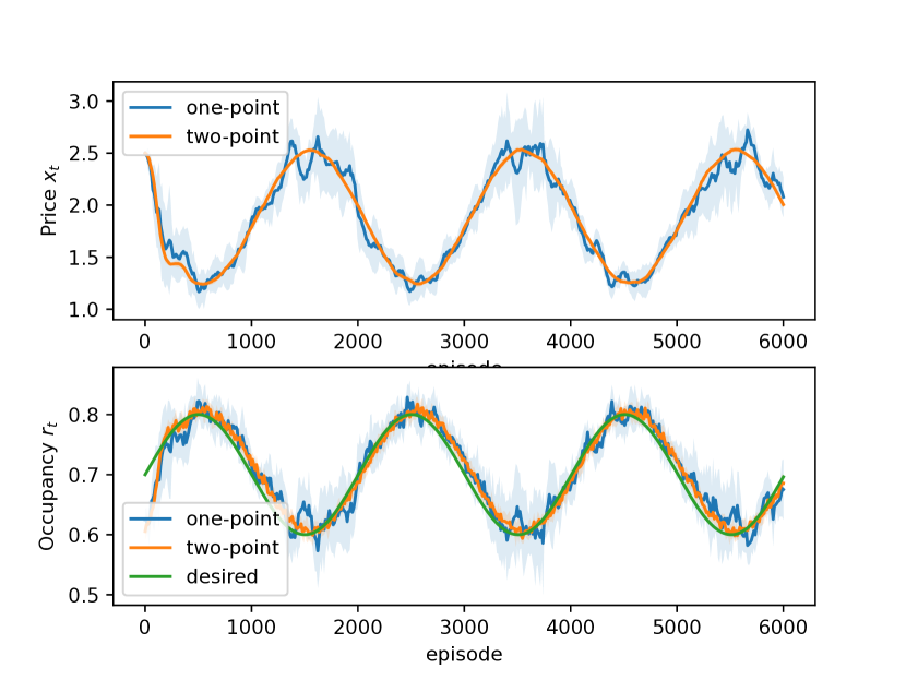
Figure 1: From top to bottom: parking prices generated by the one-point algorithm (Algorithm 1) and by the two-point algorithm (Algorithm 2); the corresponding resulting occupancies and the desired occupancy rate $r_{d}$.

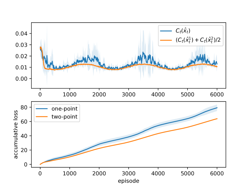
Figure 2: From top to bottom: the CVaR values under the price $\hat{x}_{t}$ generated by Algorithm 1, under the prices $\hat{x}_{t}^{1}$ and $\hat{x}_{t}^{2}$ generated by Algorithm 2; the cumulated CVaR value achieved by the one-point algorithm (Algorithm 1) and the two-point algorithm (Algorithm 2).

Fig. 3 depicts the resulting occupancies and the regret achieved by two-point risk-averse learning algorithm with maximum delay $\bar{d}=\{0,200,400\}$. The sampling number is set as $n_{t}=8$. Fig. 3 shows that, as the delay increases, the variance of the resulting occupancy and the cumulated loss both increase. Fig. 4 depicts the resulting occupancies and the regret achieved by Algorithm 2 with sampling number $n_{t}=\{1,2,16\}$ for all $t$, while fixing the maximum delay as $\bar{d}=200$. Fig. 4 shows that, as the sampling number increases, the variance of the resulting occupancy and the cumulated loss both decrease.

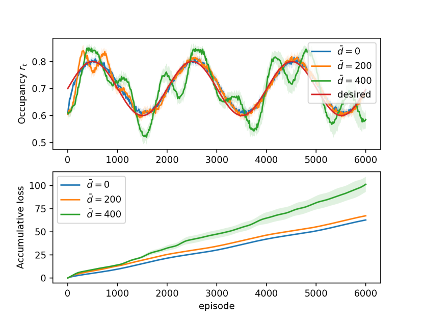
Figure 3: The occupancies and cumulated losses generated by Algorithm 2 under maximum individual delays $\bar{d}=\{0,200,400\}$.

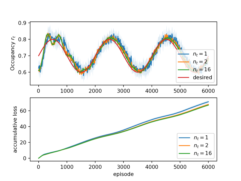
Figure 4: The occupancies and cumulated losses generated by Algorithm 2 with sample strategies $n_{t}=\{1,2,16\}$.

5 CONCLUSIONS

This paper investigated risk-averse learning with delayed feedback, where the delays are varying but bounded. We reorganized the arriving feedback into virtual time slots based on their reception order. Both one-point and two-point zeroth-order optimization approaches are utilized to estimate the CVaR gradient, with function values being queried multiple times under perturbed actions in both cases. We then developed corresponding one-point and two-point risk-averse learning algorithms based on these CVaR gradient estimates. The regret bounds of these algorithms are analyzed in terms of cumulative delay and total sampling number. The theoretical results indicate that the two-point risk-averse learning algorithm outperforms the one-point algorithm. Furthermore, the one-point algorithm achieves sublinear regret when the cumulative and individual delays meet specific bound conditions, while the two-point algorithm requires only minimal restrictions on both cumulative and individual delays.

6 Appendix

Proof. We start from the first claim. Denote $L_{\mu(\tau)-1}=m$, which means the learner receives $m$ batches feedback before $t_{1}=\mu(\tau)$. Due to the presence of delay, we have $0\leq m\leq\mu(\tau)-1$. The learner receives the $\tau$-th batch feedback at slot $t_{2}=\mu(\tau)+d_{\mu(\tau)}\geq t_{1}$. In other words, the learner receives at least $m$ batches feedback before $t_{2}$. Then, we have $\tau\geq m+1$, and further that $\tilde{s}_{\tau}\geq m+1-1-m=0$.

We next prove the second claim. According to the definition of $\tilde{s}_{\tau}$, we have

$$\sum_{\tau=1}^{L_{T}}\tilde{s}_{\tau} =\sum_{\tau=1}^{L_{T}}\big{(}\tau-1-L_{\mu(\tau)-1}\big{)}$$

$$=\sum_{t=1}^{L_{T}}(t-1)-\sum_{\tau=1}^{L_{T}}L_{\mu(\tau)-1}$$

$$=\sum_{t=1}^{L_{T}}(t-1)-\sum_{t=1}^{L_{T}-\bar{d}}L_{t-1}-\sum_{\tau\in\mathcal{S}}L_{\mu(\tau)-1},$$ (38)

with $\mathcal{S}=\{\tau|1\leq\tau\leq L_{T},\mu(\tau)>L_{T}-\bar{d}\}$. The last equality of (6) follows from separating $\sum_{\tau=1}^{L_{T}}L_{\mu(\tau)-1}$ into two parts: $L_{\mu(\tau)-1}$ for $\tau\in\{s|1\leq s\leq L_{T},\mu(s)\in\{1,\dots,L_{T}-\bar{d}\}\}$, i.e., those generated during $t\in\{1,\dots,L_{T}-\bar{d}\}$, and the remaining, i.e., $L_{\mu(\tau)-1}$, for $\tau\in\mathcal{S}$. For the first and the second term of (6), we have

$$\hskip 10.00002pt\sum_{t=1}^{L_{T}}(t-1)-\sum_{t=1}^{L_{T}-\bar{d}}L_{t-1}$$

$$=\sum_{t=1}^{L_{T}-2\bar{d}-1}t-\sum_{t=1}^{L_{T}-\bar{d}-1}L_{t}+\sum_{t=L_{T}-2\bar{d}}^{L_{T}-1}t$$

$$\leq\sum_{t=1}^{L_{T}-2\bar{d}-1}d_{t}+\sum_{t=L_{T}-2\bar{d}}^{L_{T}-1}t$$

$$=\sum_{t=1}^{L_{T}-2\bar{d}-1}d_{t}+\bar{d}(2L_{T}-2\bar{d}-1),$$ (39)

where the first equality is from $L_{0}=0$. We next explain the inequality. In the absence of delay, the learner receives $t$ batches of feedback by the end of slot $t$. Then, $\sum_{t=1}^{{L_{T}-\bar{d}-1}}t$ can be interpreted as each packet is accounted once at each slot since its arrival over the horizon $L_{T}-\bar{d}-1$. Accordingly, $\sum_{t=1}^{{L_{T}-\bar{d}-1}}L_{t}$ can be interpreted as each packet is accounted once at each slot since its arrival in the presence of delay. By Assumption 1, the losses $J_{t}(\cdot)$, for $t\in\{1,\dots,L_{T}-2\bar{d}-1\}$, arrive by end of $L_{T}-\bar{d}-1$ slot. Moreover, $J_{t}(\cdot)$ is undercounted $d_{t}$ times by slot $t+\bar{d}$. Thus, we have $\sum_{t=1}^{L_{T}-2\bar{d}-1}t-\sum_{t=1}^{L_{T}-\bar{d}-1}L_{t}\leq\sum_{t=1}^{L_{T}-2\bar{d}-1}d_{t}$. For the last term of (6), we have

$$\sum_{\tau\in\mathcal{S}}L_{\mu(\tau)-1} \geq\sum_{\tau\in\mathcal{S}}\mu(\tau)-\bar{d}-1\geq\sum_{L_{T}-2\bar{d}}^{L_{T}-\bar{d}-1}t$$

$$=\frac{\bar{d}(2L_{T}-3\bar{d}-1)}{2},$$ (40)

where the first inequality is from $L_{t}\geq t-\bar{d}$ and the second inequality is from the fact the set $\mathcal{S}$ has $\bar{d}$ components and $\mu(\tau)\geq L_{T}-\bar{d}+1$ for $\tau\in\mathcal{S}$, as in (6). Substitute (6) and (6) into (6), we obtain the second claim. $\blacksquare$

References

- [1] Adrian Rivera Cardoso and Huan Xu. Risk-averse stochastic convex bandit. In Proc. of the 22nd International Conference on Artificial Intelligence and Statistics, pages 39–47, 2019.
- [2] Ido Greenberg, Yinlam Chow, Mohammad Ghavamzadeh, and Shie Mannor. Efficient risk-averse reinforcement learning. Advances in Neural Information Processing Systems, 35:32639–32652, 2022.
- [3] Siddharth Alexander, Thomas F Coleman, and Yuying Li. Minimizing cvar and var for a portfolio of derivatives. Journal of Banking & Finance, 30(2):583–605, 2006.
- [4] Mehdi Tavakoli, Fatemeh Shokridehaki, Mudathir Funsho Akorede, Mousa Marzband, Ionel Vechiu, and Edris Pouresmaeil. Cvar-based energy management scheme for optimal resilience and operational cost in commercial building microgrids. International Journal of Electrical Power & Energy Systems, 100:1–9, 2018.
- [5] Mohamadreza Ahmadi, Xiaobin Xiong, and Aaron D Ames. Risk-averse control via cvar barrier functions: Application to bipedal robot locomotion. IEEE Control Systems Letters, 6:878–883, 2021.
- [6] Aviv Tamar, Yonatan Glassner, and Shie Mannor. Optimizing the cvar via sampling. In Proceedings of the AAAI Conference on Artificial Intelligence, volume 29, 2015.
- [7] Carlo Filippi, Gianfranco Guastaroba, and Maria Grazia Speranza. Conditional value-at-risk beyond finance: a survey. International Transactions in Operational Research, 27(3):1277–1319, 2020.
- [8] S Taymaz, C Iyigun, ZP Bayindir, and NP Dellaert. A healthcare facility location problem for a multi-disease, multi-service environment under risk aversion. Socio-Economic Planning Sciences, 71:100755, 2020.
- [9] R Tyrrell Rockafellar, Stanislav Uryasev, et al. Optimization of conditional value-at-risk. Journal of risk, 2:21–42, 2000.
- [10] Abraham D Flaxman, Adam Tauman Kalai, and H Brendan McMahan. Online convex optimization in the bandit setting: gradient descent without a gradient. arXiv preprint cs/0408007, 2004.
- [11] Yan Zhang, Yi Zhou, Kaiyi Ji, and Michael M Zavlanos. A new one-point residual-feedback oracle for black-box learning and control. Automatica, 136:110006, 2022.
- [12] Ohad Shamir. An optimal algorithm for bandit and zero-order convex optimization with two-point feedback. Journal of Machine Learning Research, 18(52):1–11, 2017.
- [13] Yurii Nesterov and Vladimir Spokoiny. Random gradient-free minimization of convex functions. Foundations of Computational Mathematics, 17(2):527–566, 2017.
- [14] John Langford, Alexander Smola, and Martin Zinkevich. Slow learners are fast. arXiv preprint arXiv:0911.0491, 2009.
- [15] Bingcong Li, Tianyi Chen, and Georgios B Giannakis. Bandit online learning with unknown delays. In The 22nd International Conference on Artificial Intelligence and Statistics, pages 993–1002. PMLR, 2019.
- [16] Amélie Héliou, Panayotis Mertikopoulos, and Zhengyuan Zhou. Gradient-free online learning in continuous games with delayed rewards. In International conference on machine learning, pages 4172–4181. PMLR, 2020.
- [17] Claire Vernade, Andras Gyorgy, and Timothy Mann. Non-stationary delayed bandits with intermediate observations. In International Conference on Machine Learning, pages 9722–9732. PMLR, 2020.
- [18] Pooria Joulani, Andras Gyorgy, and Csaba Szepesvári. Online learning under delayed feedback. In International conference on machine learning, pages 1453–1461. PMLR, 2013.
- [19] Benjamin Howson, Ciara Pike-Burke, and Sarah Filippi. Delayed feedback in generalised linear bandits revisited. In International Conference on Artificial Intelligence and Statistics, pages 6095–6119. PMLR, 2023.
- [20] Zifan Wang, Yi Shen, Zachary I Bell, Scott Nivison, Michael M Zavlanos, and Karl H Johansson. A zeroth-order momentum method for risk-averse online convex games. In Proc. of the 61st IEEE Conference on Decision and Control, pages 5179–5184. IEEE, 2022.
- [21] Aryeh Dvoretzky, Jack Kiefer, and Jacob Wolfowitz. Asymptotic minimax character of the sample distribution function and of the classical multinomial estimator. The Annals of Mathematical Statistics, pages 642–669, 1956.
- [22] Mitas Ray, Lillian J Ratliff, Dmitriy Drusvyatskiy, and Maryam Fazel. Decision-dependent risk minimization in geometrically decaying dynamic environments. In Proc. of the AAAI Conference on Artificial Intelligence, pages 8081–8088, 2022.