TorchSISSO: A PyTorch-Based Implementation of the Sure Independence Screening and Sparsifying Operator for Efficient and Interpretable Model Discovery

Abstract

Symbolic regression (SR) is a powerful machine learning approach that searches for both the structure and parameters of algebraic models, offering interpretable and compact representations of complex data. Unlike traditional regression methods, SR explores progressively complex feature spaces, which can uncover simple models that generalize well, even from small datasets. Among SR algorithms, the Sure Independence Screening and Sparsifying Operator (SISSO) has proven particularly effective in the natural sciences, helping to rediscover fundamental physical laws as well as discover new interpretable equations for materials property modeling. However, its widespread adoption has been limited by performance inefficiencies and the challenges posed by its FORTRAN-based implementation, especially in modern computing environments. In this work, we introduce TorchSISSO, a native Python implementation built in the PyTorch framework. TorchSISSO leverages GPU acceleration, easy integration, and extensibility, offering a significant speed-up and improved accuracy over the original. We demonstrate that TorchSISSO matches or exceeds the performance of the original SISSO across a range of tasks, while dramatically reducing computational time and improving accessibility for broader scientific applications.

1 Introduction

First principles models, derived from fundamental physical laws, have been instrumental in the development of scientific theories and technological systems. For example, the Navier-Stokes equation offers a comprehensive description of fluid flow, enabling predictions of complex behaviors in everything from blood flow [1] to weather patterns [2]. Traditionally, this pursuit has relied on the extensive expertise of domain specialists, requiring trial and error to identify features and model structures that fit the observations. In recent years, the landscape of scientific inquiry has been transformed by the availability of machine learning frameworks, such as neural networks, support vector machines, and Gaussian processes, which offer a powerful alternative for deriving predictive models [3]. These data-driven regression methods are often complex, do not typically generalize outside of the training set, and provide limited insights into the underlying physics. For instance, while these models may be trained to accurately predict the Reynolds number, they cannot capture the competitive nature between inertial and viscous forces in fluid flow. The only data-driven modeling framework that can provide insights comparable to first principles models, to the best of our knowledge, is symbolic regression (SR) [4, 5, 6].

SR is an automated supervised learning technique that takes a user provided operator set and initial feature space to engineer expressions by combinatorically applying the operators to the base features set. Early work in SR [4] introduced the concept of using genetic programming (GP) to discover mathematical expressions and computer programs. The framework evolves a population of mathematical equations by applying genetic operations to the fittest individuals from the space of engineered expressions. Building on this work, Eureqa [7], developed a fitness function used to evaluate and evolve the population towards a ground-truth model. The GPLearn algorithm [8] is an open source implementation that improved on Eureqa by adding custom operators and the option to include constraints. The AI-Feynman and subsequent AI-Feynman 2.0 [9, 10] build on this work by first exploiting simplifying properties of the data to to improve reliability and second returning a Pareto-optimal set of models to balance the model complexity with accuracy. Most recently, PySR [11] has proposed several modifications to the genetic-based SR frameworks. This work proposed the use of a simulated annealing to actively tune the the fitness function used for identifying the fittest individuals from the population, a model simplifying stage between evolving candidates and optimizing the model parameters, and incorporates a novel complexity metric as a penalty in the fitness function.

The approaches discussed thus far employ creative strategies to navigating the enormous spaces of possible models, due to high computation demand of exhaustive exploration. However, the these approaches are not guaranteed to find the correct model structure, as SR has been proven to be an NP-hard problem [12]. While a truly exhaustive search would not be possible, several methods have investigated strategies to perform a targeted search over the sparse models. The Sparse Identification of Nonlinear Dynamics (SINDy) method [13] uses traditional sparse regression methods over an engineered feature space to balance model complexity with prediction accuracy, mainly for dynamic systems. An important challenge with SINDy in practice is the selection of the pre-defined feature set that plays big role in the achievable performance (e.g., the method will start to struggle if too many expanded features are considered). The Sure Independence Screening and Sparsifying Operators (SISSO) method [14] instead aims to tackle the problem of working with huge feature spaces (up to $\sim 10^{9}$ candidate features) by combining a fast feature screening method with exhaustive search over the subspace of features. SISSO relies on sure independence screening (SIS) [15] to identify the most correlated features to the target using a simple dot product and a sparsity operator (typically $\ell_{0}$ regularization) to find the best simple model that fits the available training data. Recent work has also shown that SISSO can effectively be combined with other feature screening methods, such as mutual information pre-screening, to help deal with problems involving a large number of primary features/inputs before expansion [16]. Furthermore, a Python wrapper package, pysisso, was recently developed to make the FORTRAN-SISSO implementation accessible to practitioners without knowledge of the FORTRAN language [17]. However, the backend of pysisso still requires the a FORTRAN compiler, which does not fully address the difficulties with installation.

In this work, we present the TorchSISSO package, a user-friendly Python implementation of the SISSO framework designed to make the methodology accessible to a wider range of researchers and practitioners across diverse scientific fields. By eliminating the need for a FORTRAN compiler, TorchSISSO simplifies installation and usage, especially in modern computing environments. Furthermore, it allows users to easily modify the feature expansion process, which is hard-coded in the original FORTRAN implementation. This flexibility is a critical improvement, as we observed that the original SISSO does not always expand features as intended. Through simple examples, we demonstrate that TorchSISSO is capable of discovering the correct symbolic expressions in cases where the FORTRAN-based version cannot.

Additionally, the combinatorial expansion of the feature space may be slow or even infeasible, depending on the available memory. To address this issue, TorchSISSO uses parallel computing and optional GPU acceleration, providing significant computational speed up and scalability of the SISSO method. The remainder of the manuscript is organized as follows: first, we provide a detailed description of the SISSO framework in Section 2, and introduce the proposed toolbox in Section 3. In Section 4, we present performance comparison metrics for the proposed TorchSISSO to the FORTRAN-SISSO implementation. Lastly, we provide concluding remarks in Section 5.

2 The SISSO Method

The SR problem can be formulated as an empirical risk minimization over a function space $\cal F$. For given target variables $y^{(i)}\in\mathbb{R}$ and feature variables $x^{(i)}\in\mathbb{R}^{d}$ for $i\in\{1,...,N\}$ data points, the SR problem can be defined as [18]

$$f^{\star}=\operatorname*{argmin}_{f\in\mathcal{F}}\frac{1}{N}\sum_{i=1}^{N}L(f(x^{(i)}),y^{(i)}).$$ (1)

Here, $\mathcal{F}$ consists of all mappings $f:\mathbb{R}^{d}\to\mathbb{R}$ and $f^{\star}$ is the optimal model that produces the lowest average loss $L(\cdot)$, across the training data.

The main difference between classical regression methods and SR is how $\cal F$ is defined. Classical regression defines the function space by assuming a structural form $\mathcal{F}=\{f_{\theta}(x),~{}\forall\theta\in\Theta\}$, where $\theta$ is a collection of model parameters in some set $\Theta$. As long as the structures $f_{\theta}$ lead to differentiable loss functions in (1), one can then apply (stochastic) gradient descent methods to approximately solve (1) (to at least a local optimum depending on the convexity of the loss). The SISSO method, on the other hand, aims to optimize over a set $\mathcal{F}$ that is formed by function composition over a primitive set. The primitive can contain variables, algebraic operators (such as addition, subtraction, multiplication), and transcendental functions (such as exponential, square root). The set $\mathcal{F}$ then contains all valid combinations of elements of the primitive applied recursively up until some level (see, e.g., [12] for details). A key challenge with this perspective is that the size of $\mathcal{F}$ grows exponentially fast with the size of the primitive set, and this space is finite (for fixed recursion depth), such that solving (1) exactly requires exhaustive brute force search over all functions in $\mathcal{F}$.

SISSO can be thought of as an effective heuristic to exactly search over a subset of useful functions in $\mathcal{F}$. We break down our description of SISSO, originally proposed in [14], into three parts. First, we describe how feature expansion is recursively performed to build an engineered feature set that in general will be a subset of $\mathcal{F}$. Second, we summarize the sure independence screening (SIS) that identifies the very small subset of features that we want to more carefully analyze. Lastly, we present the sparsifying operator (SO) component that shows how the best functional form is selected from the subset of features identified in the previous step.

2.1 Feature Space Expansion

The choice of $\mathcal{F}$ is completely up to the user, however, in general it will contain potentially too many functions to even store in memory. Therefore, SISSO aims to recursively build a set of “expanded features” by applying a set of operators to all possible combinations of features. Let $\boldsymbol{\phi}_{0}=x$ be the initial features and let $\mathcal{O}$ denote the operator set that consists of some number of unary $o[x_{i}]$ and binary $o[x_{i},x_{j}]$ operators. Then, we define the expanded features at level $l\geq 1$ recursively as follows

$$\boldsymbol{\phi}_{l}=\{\mathcal{O}[z_{i},z_{j}],~{}~{}\forall z_{i},z_{j}\in\phi_{l-1}\}~{}~{}~{}\text{with}~{}~{}~{}\boldsymbol{\phi}_{0}=x.$$ (2)

As an example, consider the $d=2$ and a very simple operator set of $\mathcal{O}=\{I(z_{i}),z_{i}+z_{j},z_{i}\times z_{j}\}$. Then, we can construct the features up until level 2 as follows:

$$\boldsymbol{\phi}_{0} =\{x_{1},~{}x_{2}\},$$

$$\boldsymbol{\phi}_{1} =\{x_{1},~{}x_{2},~{}x_{1}+x_{2},~{}x_{1}\times x_{2}\},$$

$$\boldsymbol{\phi}_{2} =\{x_{1},~{}x_{2},~{}x_{1}+x_{2},~{}x_{1}\times x_{2},~{}2x_{1}+x_{2},~{}x_{1}+x_{1}\times x_{2},~{}x_{1}+2x_{2},~{}x_{2}+x_{1}\times x_{2},$$

$$~{}~{}~{}~{}~{}~{}~{}~{}~{}x_{1}(x_{1}+x_{2}),~{}x_{1}^{2}\times x_{2},~{}x_{2}(x_{1}+x_{2}),~{}x_{1}\times x_{2}^{2},~{}(x_{1}+x_{2}+x_{1}\times x_{2}),~{}(x_{1}+x_{2})(x_{1}\times x_{2})\}.$$

For $m_{u}$ unary operators, $m_{b,s}$ symmetric binary operators, and $m_{b,ns}$ non-symmetric binary operators, we can compute an upper bound on the number of features at any level $l\geq 1$:

$$d_{l}\leq m_{u}d_{l-1}+\left(\frac{m_{b,s}}{2}+m_{b,ns}\right)d_{l-1}(d_{l-1}-1),~{}~{}d_{0}=d.$$ (3)

Note that this is an upper bound since it is possible that some of the combinations are not unique. In the example above, we get $d_{1}\leq 2+\left(\frac{2}{2}\right)(2)(1)=4$, which is exact for the first level since all combinations are unique. For the second level, we get $d_{2}\leq 4+\left(\frac{2}{2}\right)(4)(3)=12$. This bound is larger than the 14 unique combinations shown above because we can exclude, e.g., $x_{1}+x_{2}$ and $x_{1}\times x_{2}$ that would be regenerated when expanding from level 1 to 2.

The quadratic term quickly dominates as $l$ increases such that we can write out a rough scaling law as $d_{l}\sim m_{b}^{\prime}d_{l-1}^{2}$ where $m_{b}^{\prime}=(m_{b,s}/2+m_{b,ns})$ for $l\geq 1$. Rewriting this in terms of the number of primary/starting input features, we find that the size of $\phi_{l}$ should be roughly

$$d_{l}\sim(m_{b}^{\prime})^{2^{l}-1}d^{2^{l}},$$ (4)

which grows exponentially with the number of levels $l$ (and the number of binary operators in the operator set). In practice, we can limit this growth by performing dimensional analysis during the expansion process, which restricts certain operators from being applied (e.g., addition and subtraction can only be applied if the features share the same units). However, this does place a strong limit on the maximum expansion level in SISSO – typically needs to be below 4, except in special cases. Also, note that our implementation, described in Section 3, enables the user significant flexibility in their choice of operator set $\mathcal{O}$, which plays a major role on the growth in the feature space.

2.2 Sure Independence Screening

Although higher expansion levels create a richer feature space for mapping the target, they also increase the complexity of the learning task. Specifically, finding an optimal sparse linear combination of these features becomes crucial to avoid overfitting, particularly in high-dimensional spaces. Sparsity is often achieved by applying regularization techniques in the regression process. Common strategies include $\ell_{1}$ regularization (LASSO) or a combination of $\ell_{1}$ and $\ell_{2}$ regularization (elastic net), which penalize non-zero coefficients to enforce sparsity in the model. However, selecting the appropriate hyperparameters (penalty weights) can be both challenging and time-consuming. This issue is particularly pronounced in limited data settings, where extensive validation to tune these hyperparameters is often infeasible, leading to potential model instability. The SISSO method tackles this problem by first applying sure independence screening (SIS) [15] to quickly and efficiently select a much smaller set of features for use in the modeling training/selection step.

SIS is a simple, non-parametric statistical method designed for variable selection in high-dimensional feature spaces. Variables are ranked based on the correlation magnitude metric between each feature and the target. Let $\boldsymbol{y}\in\mathbb{R}^{N}$ be the vector of training target values and $\boldsymbol{\Phi}\in\mathbb{R}^{N\times D}$ be matrix of feature values that corresponds to all $D$ features evaluated at the $N$ training input values. Note that we describe the SIS procedure for an arbitrary feature matrix that could be derived from any expansion level. Assuming the columns of $\boldsymbol{\Phi}$ have been standardized to have zero mean and unit variance, we can compute the following weights that measure the correlation between each feature and the target:

$$\boldsymbol{w}=(w_{1},\ldots,w_{D})=\boldsymbol{\Phi}^{\top}\boldsymbol{y}.$$ (5)

SIS then identifies the indices (the particular features) with the top $k$ magnitude weight:

$$\mathcal{S}=\{i\in\{1,\ldots,D\}:|w_{i}|~{}\text{is among the first $k$ largest}\}.$$ (6)

We denote this process with the shorthand: $\mathcal{S}=\text{SIS}(\boldsymbol{y},\boldsymbol{\Phi})$. Note that the choice of $k$ is up to the user; larger values will make the subsequent step more computationally demanding. We implement a default value of $k=20$ based on the recommendation from [14]. An alternative strategy is to only keep features whose correlation $w_{i}$ exceed a threshold value, which is also implemented in our TorchSISSO package.

2.3 Sparsifying Operator

Let $\boldsymbol{\phi}(x)$ denote the set of nonlinearly expanded features at any expansion level (we suppress the subscript $l$ for notational simplicity). We are aiming to find a model that is a linear combination of these features, i.e., $\boldsymbol{\phi}(x)^{\top}\boldsymbol{c}$ where $\boldsymbol{c}\in\mathbb{R}^{D}$ is a coefficient vector that we want to fit to data. Note that we assume the constant feature is included in $\boldsymbol{\phi}(x)$ to serve as a bias term in the model. Although we could fit $\boldsymbol{c}_{l}$ using standard linear regression, this problem will be underdetermined when $D>N$, which is typically the case. We also do not expect the vast majority of the features to be important when predicting $y$. SISSO thus combines SIS with a sparsifying operator (SO) to overcome this challenge.

Let $\boldsymbol{\Phi}_{\mathcal{S}}\in\mathbb{R}^{N\times k}$ denote the submatrix of feature matrix $\boldsymbol{\Phi}$ that extracts columns with indices $\mathcal{S}$. Since $k\ll D$, it is now typically possible to use standard linear regression to fit the coefficients of the $k$ remaining features. However, it is still not clear how many non-zero coefficients to retain in the model. We could address this problem using more traditional regularization methods mentioned previously, but this introduces some additional tuning parameters that are hard to select in practice. SISSO takes an alternative approach to address this issue by sequentially building models from a single term (one feature/descriptor) up until a maximum number of $T$ terms. Every time that a new term is considered, the residual error from the previous model is used to guide the chioce of the feature subset. Let $\boldsymbol{r}_{t}\in\mathbb{R}^{N}$ denote the residual error for a model with $t$ terms selected from a subset $\mathcal{S}_{t}$. It turns out that we can compute $\boldsymbol{r}_{t}$ in closed form as follows

$$\boldsymbol{r}_{t}=\boldsymbol{y}-\boldsymbol{\Phi}_{\mathcal{S}_{t}}\boldsymbol{E}_{t}\boldsymbol{c}_{t}~{}~{}~{}\text{where}~{}~{}~{}\boldsymbol{c}_{t}=(\boldsymbol{E}_{t}^{\top}\boldsymbol{\Phi}^{\top}_{\mathcal{S}_{t}}\boldsymbol{\Phi}_{\mathcal{S}_{t}}\boldsymbol{E}_{t})^{\top}\boldsymbol{E}_{t}^{\top}\boldsymbol{\Phi}^{\top}_{\mathcal{S}_{t}}\boldsymbol{y},$$ (7)

where $\boldsymbol{E}_{t}\in\mathbb{R}^{K\times t}$ is a binary matrix that selects $t$ feature columns out of the available ones in $\boldsymbol{\Phi}_{\mathcal{S}_{t}}\in\mathbb{R}^{N\times K}$, $K$ is the number of features in $\mathcal{S}_{t}$, and $\boldsymbol{c}_{t}\in\mathbb{R}^{t}$ is the coefficient vector corresponding to the least squares solution from fitting $\boldsymbol{\Phi}_{\mathcal{S}_{t}}\boldsymbol{E}_{t}$ to $\boldsymbol{y}$. Furthermore, let $\boldsymbol{r}_{t}^{\star}$ denote the residual error for the best model tested with $t$ terms from the subspace $\mathcal{S}_{t}$. SISSO recursively adds more features to the subspace as follows

$$\mathcal{S}_{t+1}=S_{t}\cup\text{SIS}(\boldsymbol{r}_{t}^{\star},\boldsymbol{\Phi})~{}~{}~{}\text{with}~{}~{}~{}\mathcal{S}_{1}=\text{SIS}(\boldsymbol{y},\boldsymbol{\Phi}).$$ (8)

In words, this procedure looks at the best $t$-term residual and then adds the next $k$ best features with the highest SIS scores with respect to the residual. We can actually compute $\boldsymbol{r}_{t}^{\star}$ using exact $\ell_{0}$ regression (or exhaustive search) over all possible $t$ term models in $\mathcal{S}_{t}$, which corresponds to the minimum $\|\boldsymbol{r}_{t}\|^{2}$ over $\binom{tk}{t}$ models. The SISSO method keeps executing (8) until the best model found for a particular $t$ achieves low enough error or until the maximum number of terms $T$ is reached. Since the number of trained models grows quickly with $T$, we typically set it to be $T=3$, meaning we at most consider 3 term models (though again this choice can be easily modified by users in our implementation). This means SISSO will attempt at most $\sum_{t=1}^{T}{\binom{tk}{t}}$ least square regression steps. The best trained model (i.e., the model with the lowest residual norm) is returned as the final model.

A simple illustration of the complete SISSO method is shown in Figure 1.

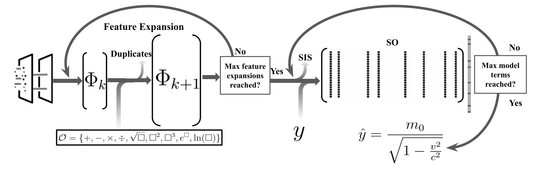
Figure 1: Illustration of the major steps in the SISSO method from [14].

3 The TorchSISSO Package

3.1 Feature pre-screening for high-dimensional problems

The original version of SISSO, outlined in Section 2, does not scale to high-dimensional primary features $x\in\mathbb{R}^{d}$, i.e., when $d$ is very large. Since this case commonly arises in practical applications (e.g., molecular property modeling), we incorporate a strategy for dealing with large $d$ in TorchSISSO. Specifically, we implement an optimal mutual information (MI) screening procedure that has been previously explored in [16, 19]. MI between a component of the primary feature vector $x_{i}$ and the target $y$ is defined as

$$\text{MI}(y;x_{i})=\int p(x_{i},y)\log\left(\frac{p(x_{i},y)}{p(x_{i})p(y)}\right)\text{d}x_{i}\text{d}y,$$ (9)

where $p(x_{i},y)$ is the joint probability density function between $x_{i}$ and $y$, $p(x_{i})$ is the marginal probability density function of $x_{i}$, and $p(y)$ is the marginal probability density function of $y$. MI is a strictly non-negative measure of the relationship between $x_{i}$ and $y$ and is only zero if $x_{i}$ and $y$ are statistically independent. In practice, we approximate the integral in (9) with kernel density estimation. MI is used to down-sample the feature space, effectively assuming that high MI implies higher likelihood that a feature contributes to the target prediction. Based on the choice by the user, we either keep the top ranked MI features up until a maximum number of terms or keep only the features whose MI fall into a specified quantile range.

3.2 PyTorch implementation

To ensure a flexible and easy to use/install package, we decided to implement the SISSO algorithm in PyTorch [20], which is an open-source machine learning library. A key feature of PyTorch is its Tensor computing framework that allows efficient implementation of multivariate tensor objects with strong acceleration using, e.g., graphics processing units (GPUs). This makes it straightforward to efficiently carry out the most expensive operations in SISSO. Looking back at Section 2, we see that SISSO mainly involves performing recursive feature expansion (2), running SIS via the matrix-vector multiplication in (5), and fitting many models with a small number of terms to find the residuals in (8). All of these steps can be straightforwardly executed using native operations in PyTorch. For feature expansion, PyTorch is highly optimized to perform efficient element-wise operations on tensors, which can be executed in parallel, leveraging the available power of the CPU or GPU for fast computation. In addition to supporting a wide variety of element-wise operations, PyTorch also enables broadcasting the result to tensors of different shapes. The torch.matmul function for matrix multiplication is generally very efficient, especially for large matrices. This makes it straightforward to execute the SIS procedure, even as the feature matrix $\boldsymbol{\Phi}$ gets very large. Lastly, the torch.linalg.lstsq function can be used to efficiently compute the residual $\boldsymbol{r}_{t}$ for a $t$-term model. Unlike many existing linear least square methods, torch.linalg.lstsq can simultaneously solve a “batch” of problems. This means we can simultaneously solve (7) for all $\binom{tk}{t}$ possible models (the different possible binary matrices $\boldsymbol{E}_{t}$), as opposed to sequentially solving each problem within a standard for loop. Note that we do not explicitly construct $\boldsymbol{E}_{t}$ and multiply it by the feature matrix, as this would be inefficient. Instead, we broadcast all possible $t$-term combinations of the features into a $B\times t\times N$ tensor where $B={\binom{tk}{t}}$ is the batch size (number of combinations of the $tk$ features split into $t$ terms), $t$ is the number of terms considered, and $N$ is the number of datapoints.

3.3 Installation and usage

The TorchSISSO package can be installed using the PIP package manager as follows

⬇

1pip install TorchSisso

endgroup The complete package is available on Github, which includes a Google Colab notebook that implements a series of simple examples using TorchSISSO that can be run interactively in the cloud. All of the core operations of TorchSISSO can be accessed using the SissoModel class that can be imported as follows

⬇

1from TorchSisso import SissoModel

To construct an instance of this class, one needs to set a number of inputs including a Pandas dataframe consisting of the training data df, the set of operators to include in the feature expansion step operators, the number of expansion levels n_expansion, the number of terms in the final model n_term, and the number of features to keep for every term in the model k. The first column of df should contain the target variable at all the training points $\boldsymbol{y}$ and the reminaing columns should contain the primary feature matrix $\boldsymbol{\Phi}_{0}=\boldsymbol{X}$ that is expanded internally to form $\boldsymbol{\Phi}_{l}$ where $l$ is equal to n_expansion. The operators should be passed in the form of a Python list, with each element being a string (for standard operators) or a function that can operate on torch.Tensor objects. We can then call the .fit() method to train the model, which returns the root mean squared error (RMSE) of the best-found model, a string version of the equation (that can easily be converted to symbolic form or a LaTeX expression), and the corresponding $R^{2}$ (coefficient of determination) value. Therefore, one can effectively train a model using SISSO with just a few lines of code:

⬇

1# import necessary packages

2import numpy as np

3import pandas as pd

4from TorchSisso import SissoModel

5# create dataframe with targets "y" and primary features "X"

6data = pd.DataFrame(np.column_stack((y, X)))

7# define unary and binary operators of interest

8operators = ["+", "-", "*", "/", "exp", "ln", "pow(2)", "sin"]

9# create SISSO model object with relevant user-defined inputs

10sm = SissoModel(data, operators, n_expansion=4, n_term=1, k=5)

11# run SISSO training algorithm to get interpretable model with highest accuracy

12rmse, equation, r2 = sm.fit()

There are two additional optional arguments that can be provided to SissoModel to help mitigate the growth of the feature space with number of expansion levels. The first is an initial_screening argument that implements the MI screening approach described in Section 3.1. The data is passed as a list of the form [method, quantile] where method="mi" indicates the use of MI screening and quantile should be a floating point number between 0 and 1 that specifies only features with MI inside of this quantile range should be kept for expansion. We also implement a simple linear correlation pre-screening method, which can be selected by setting method="spearman", though we typically find that MI performs better in practice. The second optional argument is dimensionality that should be a list of strings that represent the units of a given feature. For example, in the case that we have 5 features where features 1 to 4 have unique units while feature 5 shares the same units as feature 3, we would set this argument as dimensionality = ["u1", "u2", "u3", "u4", "u3"]. This ensures that non-physical features are not generated during the expansion process, reducing both memory usage and computational cost.

4 Numerical Examples

In this section, we compare the performance of TorchSISSO with the original SISSO implementation, referred to as FORTRAN-SISSO, and its derivatives across various test cases, including synthetic equations, challenging scientific benchmarks, and a real-world application in molecular property prediction. All results are based on a single realization of training data generated from the ground-truth equations, potentially corrupted by random observation/measurement noise. However, we found the results to be largely insensitive to the specific data realization. The experiments were run on a computing cluster with two nodes, each equipped with an Intel Xeon Gold 6444Y processor (16 cores) and 512 GB of DDR4 RAM.

4.1 Synthetic equations

We initially compare TorchSISSO to FORTRAN-SISSO on 10 synthetic expressions inspired from benchmarks commonly used in the symbolic regression (SR) literature [18]. The expressions are summarized in Table 1. For each expression, we generate 10 training datapoints by randomly sampling $x$ in $[1,5]^{d}$ where $d$ matches the number of variables appearing in the expression; all observations are corrupted with Gaussian noise with zero mean and standard deviation equal to 0.05. The computational time and the root mean squared error (RMSE) on the training set for the best-found models with TorchSISSO and FORTRAN-SISSO are shown in Table 1. We see that for several of the expressions (1, 2, 4, 6, 7, 8, 10), TorchSISSO obtains exactly the same RMSE as FORTRAN-SISSO but does so in less time. In the other three cases (3, 5, 9), TorchSISSO achieves low RMSE (indicating it has learned something very close to the ground-truth expression) while FORTRAN-SISSO learns a model with high RMSE (meaning it has failed to learn the ground truth). Case 5 is particularly interesting, as TorchSISSO finds a model with two orders of magnitude lower RMSE in nearly half the time (substantially improves in both metrics). It is not immediately obvious why FORTRAN-SISSO fails to learn the true structure for cases 3, 5, and 9; however, we believe this is due to some implementation differences in the feature expansion step. Regardless of the reason, TorchSISSO is clearly capable of achieving better performance in less time than the original FORTRAN-SISSO.

Table 1: Ground-truth models for the synthetic equations and corresponding training time and RMSE for TorchSISSO and FORTRAN-SISSO on each equation. The bold font denotes a better score and the ^⋆ denotes a tied score.

			TorchSISSO		FORTRAN-SISSO
#	Expression		Time (sec)	RMSE	Time (sec)	RMSE
1	$10\frac{x_{1}}{x_{2}(x_{3}+x_{4})}$		0.04	0.0391⋆	0.11	0.0391⋆
2	$2\sin(x_{2})+3\sqrt{x_{1}}$		0.01	0.0434⋆	0.32	0.0434⋆
3	$3\frac{\exp(x_{1})}{x_{2}+\exp(x_{3})}$		0.26	0.0342	0.20	1.4359
4	$3x_{3}+x_{2}^{2}+x_{1}^{3}$		0.27	0.0348⋆	0.57	0.0348⋆
5	$\frac{x_{2}+\exp(x_{2})}{x_{1}^{2}-x_{2}^{2}}$		0.12	0.0557	0.22	1.0786
6	$\sqrt{x_{1}^{2}+x_{2}^{2}}$		0.02	0.0646⋆	0.29	0.0646⋆
7	$\sin(x_{1}x_{3})+1.5\exp(-x_{1}x_{2})$		0.00	0.0452⋆	0.39	0.0452⋆
8	$5(x_{1}x_{3}^{3})+x_{1}^{3}+3(x_{1}x_{2}^{2})$		0.01	0.0353⋆	0.27	0.0353⋆
9	$x_{1}x_{2}x_{3}\left(\ln(x_{4})-\ln(x_{5})\right)$		66.96	1.61E-15	0.27	2.218
10	$\exp(-\frac{x_{1}}{x_{3}x_{2}})$		0.04	1.17E-16⋆	0.12	1.17E-16⋆

4.2 Scientific benchmarks

Next, we consider four equations from the SRSD-Feynman dataset [21], which is a modified version of the data proposed in [9] to have more realistic sampling ranges for the primary features and constants. Each of these equations can be found in Richard Feynman’s famous “Lectures on Physics,” and are becoming increasingly common as benchmarks for SR methods (because it mimics a realistic scientific task of discovering fundamental physical laws). The selected equations shown in Table 2 span a variety of physical phenomena including (i) the relationship between distance and two points in space, (ii) particle displacement in an electromagnetic field, (iii) relativistic mass as a function of velocity and the speed of light, and (iv) the oscillation amplitude of a charged particle in an electromagnetic field. We generate 50 training datapoints without noise using the distributions reported in [21]. The computational time and RMSE for both TorchSISSO and FORTRAN-SISSO are also shown in Table 2. Note that we use dimensional analysis in both cases to limit the growth in the expanded feature set. We see that TorchSISSO achieves the best accuracy and, in fact, discovers the exact ground truth equation in all cases. FORTRAN-SISSO, on the other hand, is unable to derive the exact equation in any of the considered cases. It is worth noting that, for the final case (oscillation amplitude), TorchSISSO does take around 42 seconds as it requires going to a third expansion level. Although this is considerably longer than the other cases, this is still substantially less time than that required by most existing SR methods (that can take several hours to find expressions of similar complexity).

Table 2: Ground-truth models for the scientific benchmarks and corresponding training time and RMSE for TorchSISSO and FORTRAN-SISSO on each equation. The bold font denotes a better score.

			TorchSISSO		FORTRAN-SISSO
Name	Physics-based Equation		Time (sec)	RMSE	Time (sec)	RMSE
Distance	$d^{2}=(x_{0}-x_{1})^{2}+(x_{2}-x_{3})^{2}$		0.40	1.35E-15	0.11	0.0363
Particle Displacement	$F=q(E+Bv\sin(\theta))$		0.21	2.1E-15	0.24	0.0449
Relativistic Mass	$m^{2}=\frac{m_{0}^{2}}{1-\frac{v_{1}^{2}}{c^{2}}}$		1.44	7.64E-6	0.13	1.185
Oscillation Amplitude	$x=\frac{qe}{m(\omega_{1}^{2}-\omega_{2}^{2})}$		42.25	6.31E-23	0.17	0.0402

4.3 Interpretable models for molecular property prediction

As a final case study, we focus on constructing simple, interpretable models for predicting molecular properties – an essential challenge in fields such as pharmaceuticals, materials science, and environmental science. Here, we look at modeling the specific energy of organic compounds, which is a property that is known to be strongly correlated to energy density when the material is used as an electrode in batteries [22]. Specific energy can be computed using the following equation

$$\text{Specific Energy}=\frac{(E-E_{\text{anode}})nF}{3600M_{W}},$$ (10)

where $E$ is the redox potential, $E_{\text{anode}}$ is the redox potential of the anode (in this case a Zinc anode), $n$ is the number of moles of electrons transferred, $F$ is Faraday’s constant, and $M_{W}$ is the molecular weight of the molecule. All quantities in (10) are known except for $E$, which can be approximated using density functional theory (DFT). The challenge, however, is that DFT is computationally expensive, making it impractical to scale (10) to millions of candidate molecules. Larger candidate sets are essential when the goal is to discover multiple high-performance molecules. To address this, we construct our training set by sampling data from a literature database presented in [23]. Specifically, we use results for 115 paraquinone molecules as our training set and reserve 1,000 quinone molecules for testing. A crucial step in building molecular property models is featurization, which involves selecting a suitable representation of molecular structure for computational analysis. For this purpose, we use the open-source PaDEL package [24] to compute 1,445 molecular descriptors for each molecule. These descriptors range from basic features, such as atom counts and molecular weight, to more complex graph-based properties. Given the high dimensionality of this problem ($d=1445$), traditional SISSO is not applicable. To manage this, we employ the mutual information (MI) screening approach in TorchSISSO, using the setting initial_screening = ["mi", 0.01] to retain only the top 1% of descriptors by MI value, which reduces the feature set to 11 out of the original 1,445. For comparison, we evaluate TorchSISSO against VS-SISSO [25], an extension of SISSO designed for high-dimensional problems that uses pre-screening. Note that VS-SISSO relies on the original FORTRAN-SISSO code for backend computations, making it a useful benchmark for our case study.

The training and testing results for both TorchSISSO and VS-SISSO are shown in Figure 2. We see that both approaches are able to obtain good training performance, with TorchSISSO and VS-SISSO achieving $R^{2}$ values of 0.985 and 0.936, respectively. However, we see a bigger difference on the test data wherein TorchSISSO and VS-SISSO achieve $R^{2}$ values of 0.932 and 0.604, respectively. In particular, VS-SISSO shows a significant drop in performance for specific energy values below 0.75 where it clearly has a biased over-prediction in this range. TorchSISSO, on the other hand, has a much tighter parity plot throughout the full range of specific energy values, implying it has learned an equation that generalizes much better beyond than the training dataset.

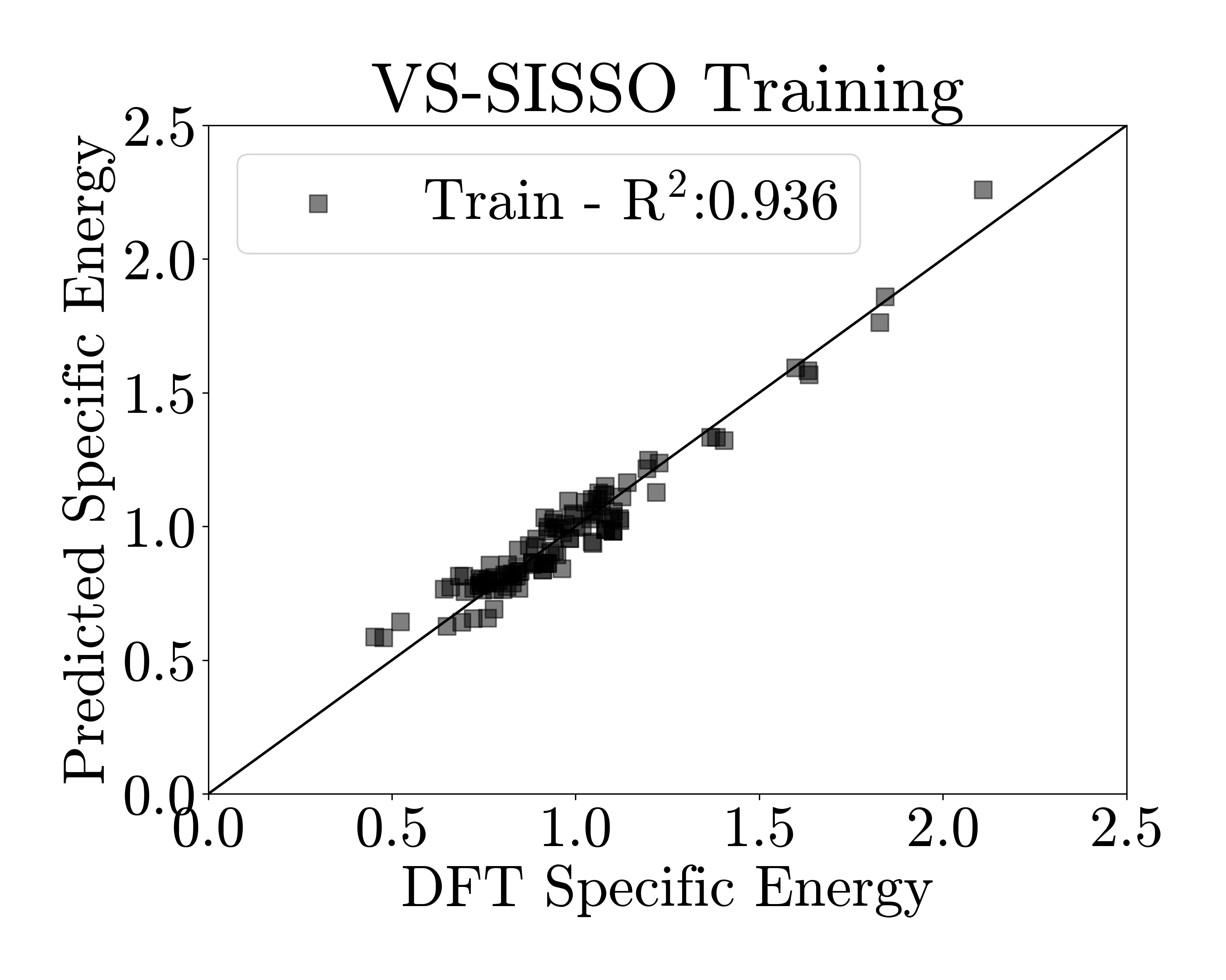
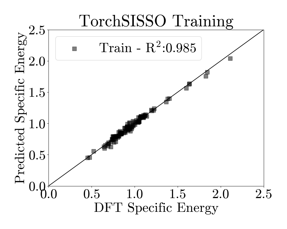
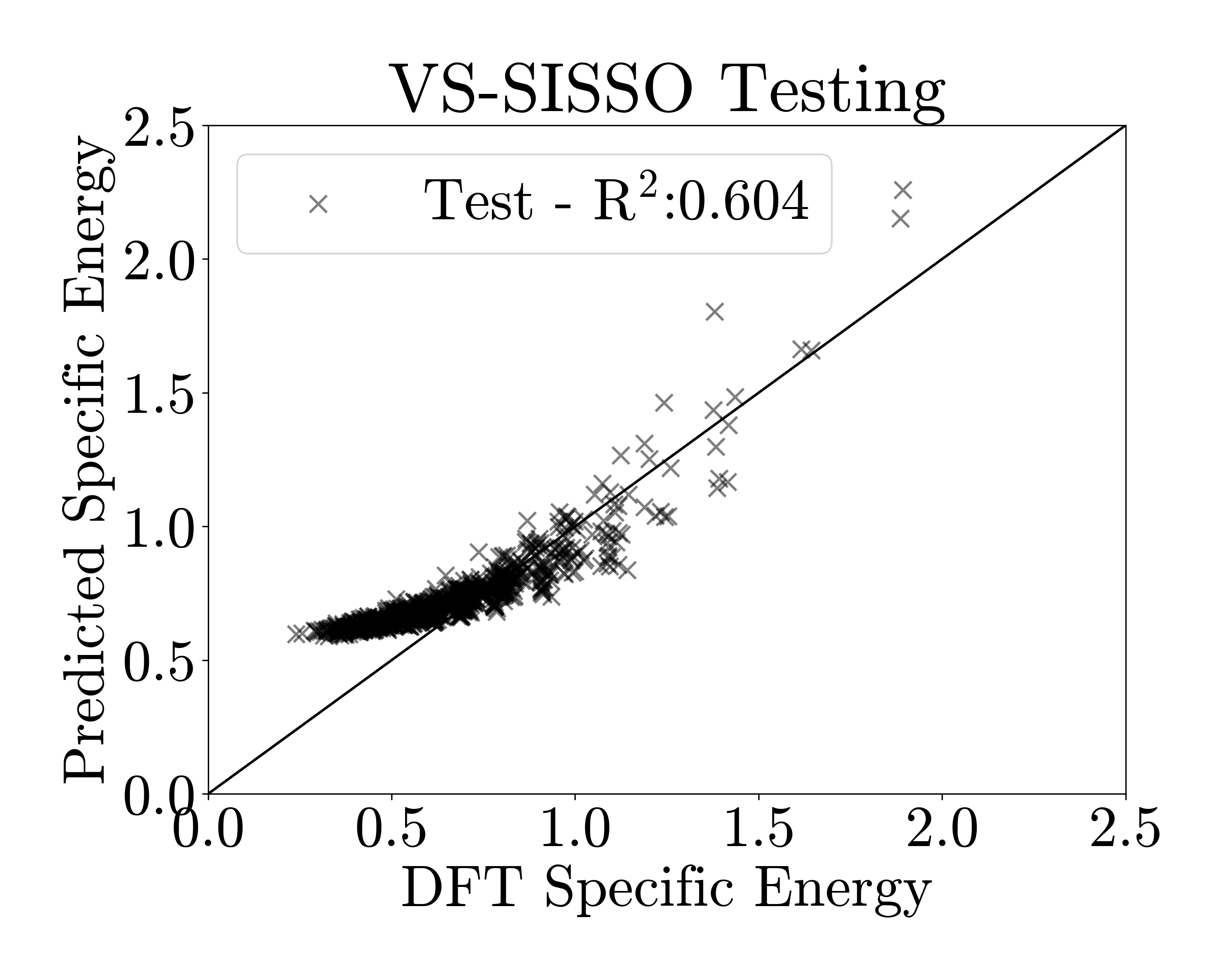
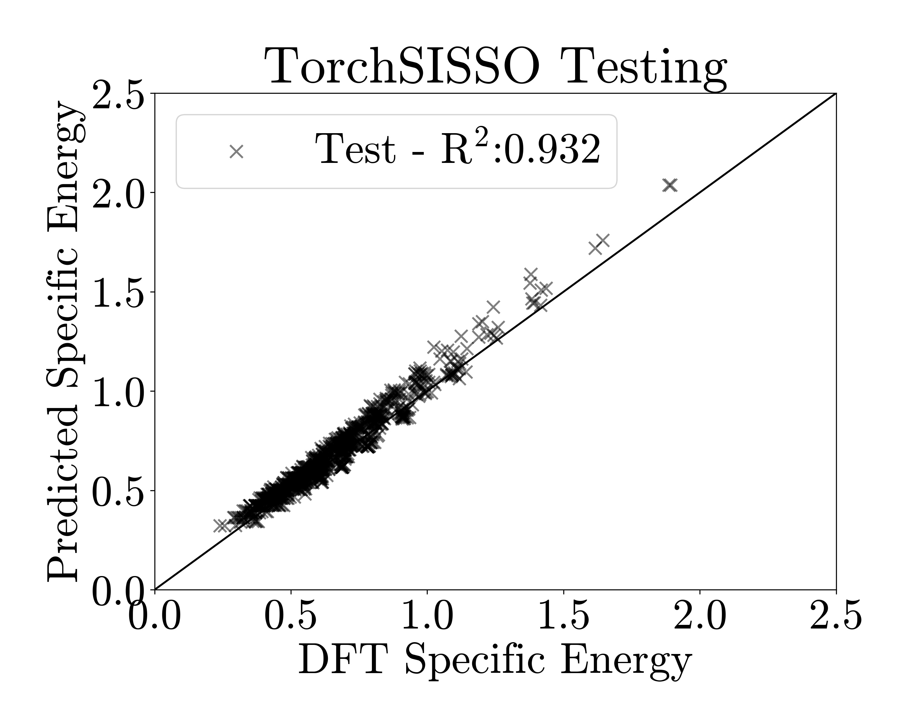
Figure 2: Results for TorchSISSO and VS-SISSO on training (top) and testing (bottom) datasets for modeling specific energy of organic compounds.

The equation found by TorchSISSO can be expressed as follows:

$$\text{Specific Energy}\approx 144.14676\left(\frac{P_{GH}+\lambda_{M}}{M_{W}\times P_{GH}}\right)+0.06388,$$ (11)

where $P_{GH}$ is the solute gas-hexadecane partition coefficient, $\lambda_{M}$ is the largest absolute eigenvalue of the Burden modified matrix weighted by relative mass, and $M_{W}$ is molecular weight. One interesting thing to notice right away is that (11) has exactly the same $M_{W}$ term in the denominator as (10) – we emphasize that this structure was not imposed during the training process, but was uncovered directly from the data. Although the other two features $P_{GH}$ and $\lambda_{M}$ are not quite as intuitive, they do carry physical significance. For example, $P_{GH}$ provides a measure of how a molecule interacts with solvents, which can impact the electronic properties (such as redox potential). Despite starting with a large and complex set of potential descriptors, TorchSISSO was able to pinpoint a compact, interpretable equation that relies on just three fundamental molecular features, combined in a simple form, to achieve high predictive accuracy on both the training and test sets. Furthermore, the specific implementation choices clearly result in an improvement over the state-of-the-art VS-SISSO code for at least this real-world example.

5 Conclusions

In this work, we introduced TorchSISSO, a native Python implementation of the Sure Independence Screening and Sparsifying Operator (SISSO) method, designed to overcome the limitations of the original FORTRAN-based implementation. By leveraging the PyTorch framework, TorchSISSO provides enhanced flexibility, allowing users to easily modify the feature expansion process and integrate modern computational resources such as GPUs for significant speed-ups. This adaptability removes barriers to install ation and usage, particularly in cloud-based or high-performance computing environments, making the SISSO method accessible to a broader scientific community.

Our results demonstrate that TorchSISSO performs comparably or better than the original SISSO implementation across a range of tasks, including synthetic test equations, scientific benchmarks, and real-world applications such as molecular property prediction. Notably, TorchSISSO shows improved accuracy in discovering true symbolic expressions in cases where the original FORTRAN-SISSO implementation falters. Additionally, the reduction in computational time, achieved through parallel processing and optional GPU acceleration, makes TorchSISSO a highly scalable tool for symbolic regression tasks on larger datasets and more complex feature spaces.

In summary, TorchSISSO addresses the key limitations of the original SISSO method, offering a faster, more accessible, and more adaptable solution for symbolic regression across a wide range of scientific fields. We believe this tool will facilitate the discovery of interpretable models in materials science, physics, and beyond, while also empowering researchers to further customize the method to fit specific domain needs. Future work will focus on extending the functionality of TorchSISSO, including multi-objective optimization, advanced regularization techniques, and automated hyperparameter tuning to further enhance its applicability.

References

- [1] Charles S Peskin. Flow patterns around heart valves: A numerical method. Journal of Computational Physics, 10(2):252–271, 1972.
- [2] Norman A. Phillips. Numerical weather prediction. Advances in Computers, 1:43–90, 1960.
- [3] Akshaya Karthikeyan and U. Deva Priyakumar. Artificial intelligence: machine learning for chemical sciences. Journal of Chemical Sciences, 134(1):2, Dec 2021.
- [4] John R. Koza. Genetic programming as a means for programming computers by natural selection. Statistics and Computing, 4(2):87–112, Jun 1994.
- [5] Yiqun Wang, Nicholas Wagner, and James M Rondinelli. Symbolic regression in materials science. MRS Communications, 9(3):793–805, 2019.
- [6] William La Cava, Bogdan Burlacu, Marco Virgolin, Michael Kommenda, Patryk Orzechowski, Fabrício Olivetti de França, Ying Jin, and Jason H Moore. Contemporary symbolic regression methods and their relative performance. Advances in Neural Information Processing Systems, 2021(DB1):1, 2021.
- [7] Michael Schmidt and Hod Lipson. Distilling free-form natural laws from experimental data. Science, 324(5923):81–85, 2009.
- [8] T. Stephens. gplearn: Genetic programming in python, with a scikit-learn inspired api, 2015.
- [9] Silviu-Marian Udrescu and Max Tegmark. Ai feynman: a physics-inspired method for symbolic regression, 2020.
- [10] Silviu Marian Udrescu, Andrew Tan, Jiahai Feng, Orisvaldo Neto, Tailin Wu, and Max Tegmark. Ai feynman 2.0: Pareto-optimal symbolic regression exploiting graph modularity. In H. Larochelle, M. Ranzato, R. Hadsell, M.F. Balcan, and H. Lin, editors, Advances in Neural Information Processing Systems, volume 33, pages 4860–4871. Curran Associates, Inc., 2020.
- [11] Miles Cranmer. Interpretable machine learning for science with pysr and symbolicregression.jl, 2023.
- [12] Marco Virgolin and Solon P. Pissis. Symbolic regression is np-hard, 2022.
- [13] Steven L. Brunton, Joshua L. Proctor, and J. Nathan Kutz. Discovering governing equations from data by sparse identification of nonlinear dynamical systems. Proceedings of the National Academy of Sciences, 113(15):3932–3937, 2016.
- [14] Runhai Ouyang, Stefano Curtarolo, Emre Ahmetcik, Matthias Scheffler, and Luca M. Ghiringhelli. Sisso: A compressed-sensing method for identifying the best low-dimensional descriptor in an immensity of offered candidates. Phys. Rev. Mater., 2:083802, Aug 2018.
- [15] Jianqing Fan. Sure independence screening for ultrahighdimensional feature space. Journal of the Royal Statistical Society, 2008.
- [16] Yuqin Xu and Quan Qian. i-sisso: Mutual information-based improved sure independent screening and sparsifying operator algorithm. Engineering Applications of Artificial Intelligence, 116:105442, 2022.
- [17] David Waroquiers. Pysisso.
- [18] Nour Makke and Sanjay Chawla. Interpretable scientific discovery with symbolic regression: a review. Artificial Intelligence Review, 57(1):2, 2024.
- [19] Roberto Battiti. Using mutual information for selecting features in supervised neural net learning. IEEE Transactions on Neural Networks, 5(4):537–550, 1994.
- [20] Adam Paszke, Sam Gross, Francisco Massa, Adam Lerer, James Bradbury, Gregory Chanan, Trevor Killeen, Zeming Lin, Natalia Gimelshein, Luca Antiga, and A. Desmaison. Pytorch: An imperative style, high-performance deep learning library. Advances in Neural Information Processing Systems, 32, 2019.
- [21] Yoshitomo Matsubara, Naoya Chiba, Ryo Igarashi, and Yoshitaka Ushiku. Rethinking symbolic regression datasets and benchmarks for scientific discovery. arXiv preprint arXiv:2206.10540, 2022.
- [22] Madison R Tuttle, Emma M Brackman, Farshud Sorourifar, Joel Paulson, and Shiyu Zhang. Predicting the solubility of organic energy storage materials based on functional group identity and substitution pattern. The Journal of Physical Chemistry Letters, 14(5):1318–1325, 2023.
- [23] Daniel P Tabor, Rafael Gómez-Bombarelli, Liuchuan Tong, Roy G Gordon, Michael J Aziz, and Alán Aspuru-Guzik. Mapping the frontiers of quinone stability in aqueous media: implications for organic aqueous redox flow batteries. Journal of Materials Chemistry A, 7(20):12833–12841, 2019.
- [24] Chun Wei Yap. Padel-descriptor: An open source software to calculate molecular descriptors and fingerprints. Journal of Computational Chemistry, 32(7):1466–1474, 2011.
- [25] Zhen Guo, Shunbo Hu, Zhong-Kang Han, and Runhai Ouyang. Improving symbolic regression for predicting materials properties with iterative variable selection. Journal of Chemical Theory and Computation, 18(8):4945–4951, Aug 2022.